
Multi-Objective Green Closed-Loop Supply Chain Management with Bundling Strategy, Perishable Products, and Quality Deterioration

Abstract
:1. Introduction
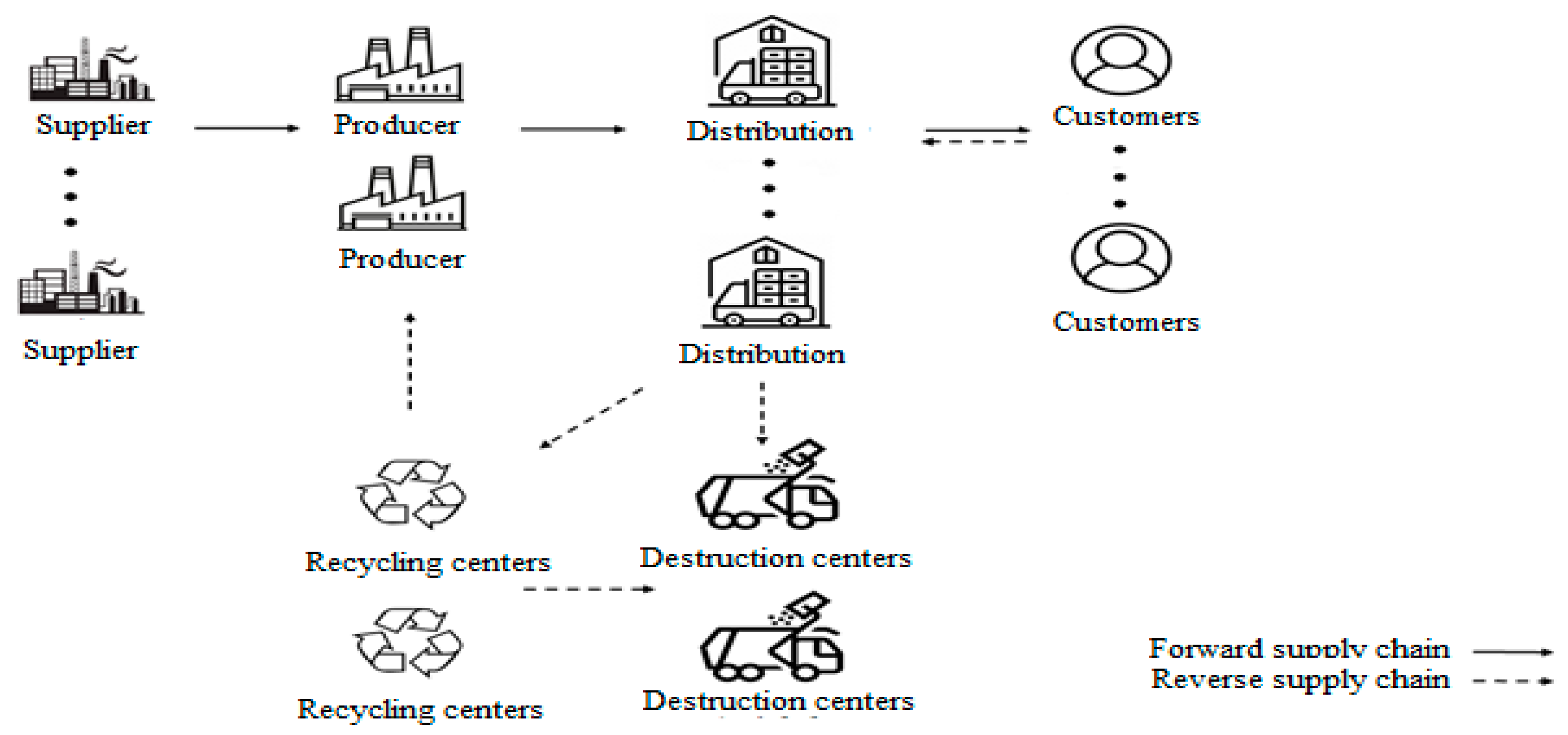
- Presenting a mathematical model of a CLSC encompassing the vectors of destruction and recycling of products under cost, time, pollutant, and risk reduction conditions.
- Considering the parts related to destruction and recycling under conditions of uncertainty, depending on the quality of the products, within a CLSC. Hence, the quality level of the returned products from the customer’s side is evaluated, and based on the evaluation results, decisions are made regarding recycling or destruction.
2. Literature Review
3. Mathematical Modeling
3.1. Proposed Model Assumptions
- The problem represents a multi-objective, single-period, and multi-product model.
- All customer demands must be met.
- Material flow can only be established between two different levels of the network, and there is no material flow between facilities in one layer.
- The capacity of the facility is limited.
- The suppliers’ location, production, distribution, collection, recycling, annihilation centers, and customers are known.
- A part of returned products is recycled in the reverse supply chain and returned back into the chain, while part of it is excreted and removed from the network.
- The packaging products’ sales volume is usually greater than that of individual sold goods due to the lower price of packaging products than the total price of individual items combined.
- The productive–technical risk considered in the proposed network model includes interruptions caused by equipment failure and a shortage of skilled labor.
- Considering the uncertainties of demand in the real world, customer demand is uncertain in the model as well.
- The amount of products returned from customers and the rates of recycling and destruction are considered uncertain. Disposal refers to the return of a product that enters the recycling stage, but destruction means returning the product to the destruction center. In fact, a product that cannot be recycled is transferred to the destruction center instead of the disposal center.
3.2. Notations and Formulations
- ➢
- Sets:
| The entire sales period | |
| Suppliers set | |
| Products set | |
| Production centers | |
| Customers | |
| Distribution-collection centers | |
| Annihilation centers | |
| Recycling centers | |
| Staff | |
| Equipment set | |
| Vehicle types | |
| Decision cycle, pricing, and packaging phases |
- ➢
- Parameters:
| Number of type products produced in period | |
| Inventory cost of type product per decision period | |
| Product inventory in period | |
| Product logistics cost | |
| Purchasing costs for each raw material unit from supplier | |
| Raw material transportation costs from supplier to production center utilizing type vehicle depending on distance | |
| Product transportation costs from the production center to the distribution-collection center by type vehicle depending on distance | |
| Product transportation costs from the distribution–collection center to customer by type vehicle depending on distance | |
| Transportation costs for the returned products from customer to the distribution–collection center by type vehicle depending on distance | |
| Transportation costs for the returned products from the distribution–collection center to the recycling center by type vehicle depending on distance | |
| Transportation costs for the returned products from the distribution–collection center to the annihilation center by type vehicle depending on distance | |
| Transportation costs for the recycled products from the recycling center to the production center by type vehicle depending on distance | |
| Transportation costs for the returned products from the recycling center to the annihilation center by type vehicle depending on distance | |
| Maintenance costs of type products in the distribution–collection center | |
| Equipment repair and maintenance costs | |
| Cost of staff training | |
| Recycling costs of type products at the recycling center | |
| Costs of annihilating type products in the annihilation center | |
| Delay costs per time | |
| Inspection costs for each returned product unit in the distribution–collection center | |
| Purchasing costs for each unit of type product from customer | |
| Renting costs for a car type | |
| Purchasing costs for a car type | |
| Person–hour needed to manufacture each type product unit at the first production center | |
| Person–hour needed to manufacture each type product unit at the second production center | |
| Working hours during the order period at the first production center | |
| Working hours during the order period at the second production center | |
| Number of existing workers in the first production center | |
| Number of existing workers in the second production center | |
| Number of hired workers in the first production center | |
| Number of hired workers in the second production center | |
| Transport-related emission rates from supplier to the production center of per product unit | |
| Transport-related emission rates from the production center to the distribution–collection center per product unit | |
| Transport-related emission rates from the distribution–collection center to customer per product unit | |
| Transport-related emission rates from customer to the distribution–collection center per product unit | |
| Transport-related emission rates from the distribution–collection center to the recycling center per product unit | |
| Transport-related emission rates from the recycling center to the production center per product unit | |
| Transport-related emission rates from the recycling center to the annihilation center per product unit | |
| Transport-related emission rates from the distribution–collection center to the annihilation center per product unit | |
| emission rates for producing each type product unit | |
| emission rates for the recycling process of each type returned product unit | |
| emission rates for the annihilation process of each type returned product unit | |
| emission rates for the returned product inspection process in the distribution–collection center | |
| Supplier to the production center distance | |
| Production center to the distribution–collection center distance | |
| Distribution–collection center to client distance | |
| Client to the distribution–collection center distance | |
| Distribution–collection center to the recycling center distance | |
| Recycling center to the production center distance | |
| Recycling center to the annihilation center distance | |
| Distribution–collection center to the annihilation center distance | |
| Maximum capacity for supplier | |
| Maximum capacity for the production center | |
| Maximum capacity for the distribution–collection center | |
| Maximum capacity for the recycling center | |
| Maximum capacity for the annihilation center | |
| Maximum allowable emissions from production | |
| Maximum allowable production–technical risk | |
| Maximum acceptable delivery time for customer | |
| Customer demand | |
| Raw materials’ demand of the production center from supplier | |
| Device failure risk | |
| emission rate of total production at the production center | |
| Total time from supplying raw materials from supplier to sending final product to customer | |
| Length of time for supplying raw materials from supplier to the production center | |
| Length of time for finished products to be sent from the production center to the distribution–collection center | |
| Length of time for sending the finished product from the distribution–collection center to customer | |
| Product return rate | |
| Product return rate from the distribution–collection center to the annihilation center | |
| Product return rate from the distribution–collection center to the recycling center | |
| Recycled product sending rate from the recycling center to the production center | |
| Recycled product sending rate from the recycling center to the annihilation center | |
| Customer expected quality | |
| Quality level of the product that leads to transfer from the distribution–collection center to the annihilation center | |
| Quality level of the product that leads to transfer from the distribution–collection center to the recycling center | |
| Quality level of the product level that leads to transfer from the recycling center to the annihilation center |
Model’s Decision Variables
- ➢
- Continuous Decision Variables:
| Sale price of product in cycle | |
| Raw material amounts sent from supplier to the production center | |
| Type product amounts sent from the production center to the distribution–collection center | |
| Type product amounts sent from the distribution–collection center to customer μ | |
| Type product amounts sent from customer μ to the distribution–collection center | |
| Type product amounts delivered from the distribution–collection center to the recycling center | |
| Recycled product amounts delivered from the recycling center to the production center | |
| Product amounts delivered from the recycling center to the annihilation center | |
| Returned product amounts delivered from the distribution–collection center to the annihilation center | |
| Time to send raw materials from supplier to the production center | |
| Time to send product from the production center to the distribution–collection center | |
| Time to send product from the distribution–collection center to customer | |
| Returned rate of product with quality level from customer | |
| Returned product amounts considering quality level from customer to the distribution–collection center |
- ➢
- Binary Variables:
| If supplier is chosen, it is equal to ; otherwise, it equals . | |
| If the production center is chosen, it is equal to ; otherwise, it equals . | |
| If the distribution–collection center is chosen, it is equal to ; otherwise, it equals. | |
| If customer is chosen, it is equal to ; otherwise, it equals . | |
| If the recycling center is chosen, it is equal to ; otherwise, it equals . | |
| If the annihilation center is chosen, it is equal to ; otherwise, it equals . | |
| If the vehicle type is sent, it is equal to ; otherwise, it equals . | |
| If the vehicle type is rented, it is equal to ; otherwise, it equals . | |
| If the vehicle type is purchased, it is equal to ; otherwise, it equals . | |
| If equipment is used, it is equal to ; otherwise, it equals . |
3.3. Objective Functions
3.4. Constraints
4. Numerical Example and Results
4.1. Numerical Example
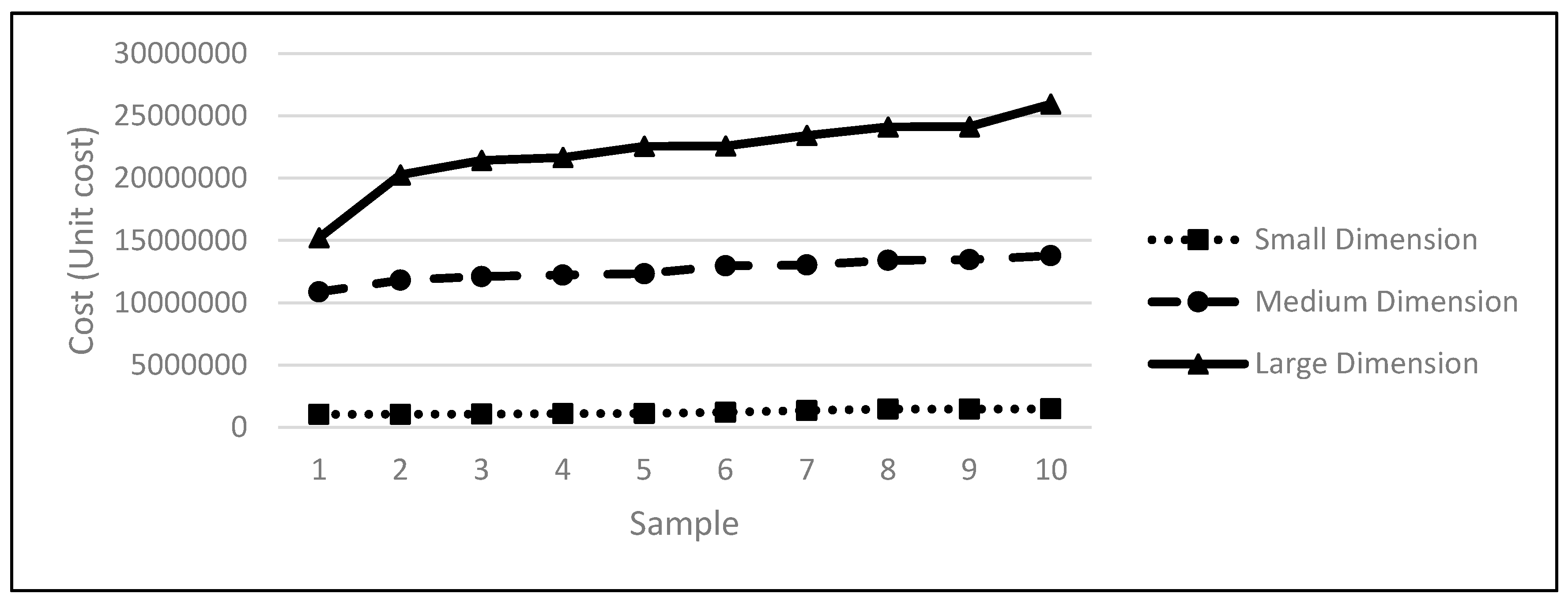
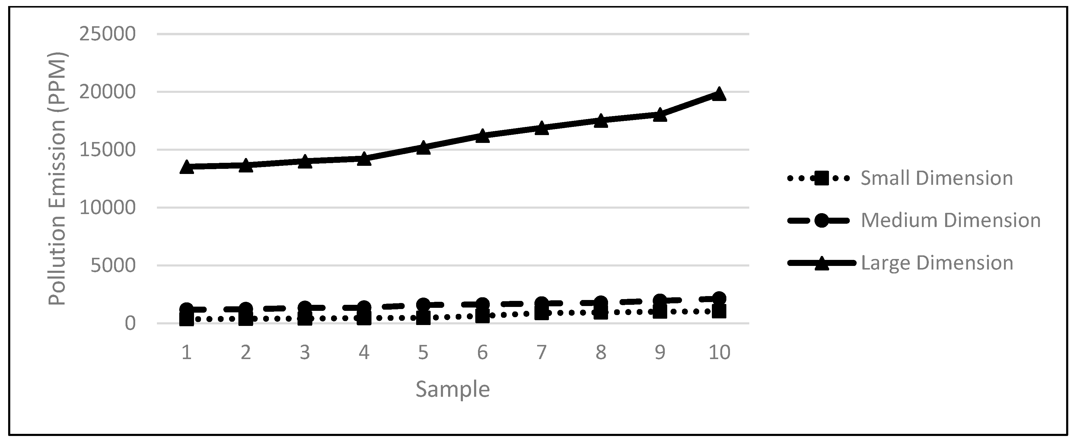
4.2. Different Sample Size Solution
4.3. Sensitivity Analysis
4.4. Comparison
5. Discussion and Conclusions
Author Contributions
Funding
Data Availability Statement
Conflicts of Interest
References
- Alzoubi, H.M.; Ghazal, T.M.; Sahawneh, N.; Al-kassem, A.H. Fuzzy assisted human resource management for supply chain management issues. Ann. Oper. Res. 2022, 326, 125004644. [Google Scholar]
- Rolf, B.; Jackson, I.; Müller, M.; Lang, S.; Reggelin, T.; Ivanov, D. A review on reinforcement learning algorithms and applications in supply chain management. Int. J. Prod. Res. 2022, 61, 7151–7179. [Google Scholar] [CrossRef]
- Boskabadi, A.; Mirmozaffari, M.; Yazdani, R.; Farahani, A. Design of a distribution network in a multi-product, multi-period green supply chain system under demand uncertainty. Sustain. Oper. Comput. 2022, 3, 226–237. [Google Scholar] [CrossRef]
- Chen, J.; Wang, H.; Fu, Y. A multi-stage supply chain disruption mitigation strategy considering product life cycle during COVID-19. Environ. Sci. Pollut. Res. 2022, 1–15. [Google Scholar] [CrossRef]
- Roh, T.; Noh, J.; Oh, Y.; Park, K.S. Structural relationships of a firm’s green strategies for environmental performance: The roles of green supply chain management and green marketing innovation. J. Clean. Prod. 2022, 356, 131877. [Google Scholar] [CrossRef]
- Abir, A.S.; Bhuiyan, I.A.; Arani, M.; Billal, M.M. Multi-Objective Optimization for Sustainable Closed-Loop Supply Chain Network Under Demand Uncertainty: A Genetic Algorithm. arXiv 2020, arXiv:2009.06047. [Google Scholar]
- Arani, M.; Liu, X.; Abdolmaleki, S. Scenario-based simulation approach for an integrated inventory blood supply chain system. In Proceedings of the 2020 Winter Simulation Conference (WSC), Orlando, FL, USA, 14–18 December 2020; pp. 1348–1359. [Google Scholar]
- Large, R.O.; Thomsen, C.G. Drivers of Green Supply Management Performance: Evidence from Germany. J. Purch. Supply Manag. 2016, 17, 176–184. [Google Scholar] [CrossRef]
- Zhu, Q.; Sarkis, J.; Lai, K.H. Green Supply Chain Management Practices and Sustainability Performance. J. Purch. Supply Manag. 2015, 19, 106–117. [Google Scholar] [CrossRef]
- Jabbarzadeh, A.; Haughton, M.; Khosrojerdi, A. Closed-loop Supply Chain Network Design under Disruption Risks: A Robust Approach with Real World Application. Comput. Ind. Eng. 2018, 116, 178–191. [Google Scholar] [CrossRef]
- Devika, K.; Jafarian, A.; Nourbakhsh, V. Designing a sustainable closed-loop supply chain network based on triple bottom line approach: A comparison of metaheuristics hybridization techniques. Eur. J. Oper. Res. 2014, 235, 594–615. [Google Scholar] [CrossRef]
- Farrokh, M.; Azar, A.; Jandaghi, G.; Ahmadi, E. A novel robust fuzzy stochastic programming for closed loop supply chain network design under hybrid uncertainty. Fuzzy Sets Syst. 2018, 341, 69–91. [Google Scholar] [CrossRef]
- Liu, M.; Liu, R.; Zhu, Z.; Chu, C.; Man, X. A bi-objective green closed loop supply chain design problem with uncertain demand. Sustainability 2018, 10, 967. [Google Scholar] [CrossRef]
- Mohtashami, Z.; Aghsami, A.; Jolai, F. A green closed loop supply chain design using queuing system for reducing environmental impact and energy consumption. J. Clean. Prod. 2020, 242, 118452. [Google Scholar] [CrossRef]
- Rezae, S.; Kheirkhah, A. A comprehensive approach in designing a sustainable closed-loop supply chain network using cross-docking operations. In Computational and Mathematical Organization Theory; Springer Science + Business Media: New York, NY, USA, 2017. [Google Scholar]
- Garai, A.; Chowdhury, S.; Sarkar, B.; Roy, T.K. Cost-effective subsidy policy for growers and biofuels-plants in closed-loop supply chain of herbs and herbal medicines: An interactive bi-objective optimization in T-environment. Appl. Soft Comput. 2021, 100, 106949. [Google Scholar] [CrossRef]
- Jerbiaa, R.; Kchaou Boujelbenb, M.; Amine Sehlia, M.; Jemaia, Z. A stochastic closed-loop supply chain network design problem with multiple recovery options. Comput. Ind. Eng. 2018, 118, 23–32. [Google Scholar] [CrossRef]
- Santander, P.; Sanchez, F.A.C.; Boudaoud, H.; Camargo, M. Closed loop supply chain network for local and distributed plastic recycling for 3D printing: A MILP-based optimization approach. Resources. Conserv. Recycl. 2020, 154, 104531. [Google Scholar] [CrossRef]
- Goodarzian, F.; Hosseini-Nasab, H.; Fakhrzad, M.B. A Multi-objective Sustainable Medicine Supply Chain Network Design Using a Novel Hybrid Multi-Objective Metaheuristic Algorithm. Int. J. Eng. 2020, 33, 1986–1995. [Google Scholar] [CrossRef]
- Zarbakhshnia, N.; Kannan, D.; Mavi, R.K. Annals of Operations Research A novel sustainable multi-objective optimization model for forward and reverse logistics system under demand uncertainty. Ann. Oper. Res. 2020, 295, 843–880. [Google Scholar] [CrossRef]
- Nasr, A.K.; Tavana, M.; Alavi, B.; Mina, H. A novel fuzzy multi-objective circular supplier selection and order allocation model for sustainable closed-loop supply chains. J. Clean. Prod. 2021, 287, 124994. [Google Scholar] [CrossRef]
- Jian, J.; Li, B.; Zhang, N.; Su, J. Decision-making and coordination of green closed-loop supply chain with fairness concern. J. Clean. Prod. 2021, 298, 126779. [Google Scholar] [CrossRef]
- Tavana, M.; Kian, H.; Nasr, A.K.; Govindan, K.; Mina, H. A comprehensive framework for sustainable closed-loop supply chain network design. J. Clean. Prod. 2022, 332, 129777. [Google Scholar] [CrossRef]
- Cheng, P.; Ji, G.; Zhang, G.; Shi, Y. A closed-loop supply chain network considering consumer’s low carbon preference and carbon tax under the cap-and-trade regulation. Sustain. Prod. Consum. 2022, 29, 614–635. [Google Scholar] [CrossRef]
- Kouchaki Tajani, E.; Ghane Kanafi, A.; Daneshmand-Mehr, M.; Hosseinzadeh, A.A. A Robust Green Multi-Channel Sustainable Supply Chain based on RFID technology with considering pricing strategy and subsidizing policies. J. Ind. Eng. Int. 2022, 18, 43–78. [Google Scholar]
- Babaeinesami, A.; Tohidi, H.; Ghasemi, P.; Goodarzian, F.; Tirkolaee, E.B. A closed-loop supply chain configuration considering environmental impacts: A self-adaptive NSGA-II algorithm. Appl. Intell. 2022, 52, 13478–13496. [Google Scholar] [CrossRef]
- Alinezhad, M.; Mahdavi, I.; Hematian, M.; Tirkolaee, E.B. A fuzzy multi-objective optimization model for sustainable closed-loop supply chain network design in food industries. Environ. Dev. Sustain. 2022, 1–28. [Google Scholar] [CrossRef]
- Bathaee, M.; Nozari, H.; Szmelter-Jarosz, A. Designing a new location-allocation and routing model with simultaneous pick-up and delivery in a closed-loop supply chain network under uncertainty. Logistics 2023, 7, 3. [Google Scholar] [CrossRef]
- Wang, Z.; Zhen, H.L.; Deng, J.; Zhang, Q.; Li, X.; Yuan, M.; Zeng, J. Multiobjective optimization-aided decision-making system for large-scale manufacturing planning. IEEE Trans. Cybern. 2021, 52, 8326–8339. [Google Scholar] [CrossRef]
- Leung, M.F.; Coello, C.A.C.; Cheung, C.C.; Ng, S.C.; Lui, A.K.F. A hybrid leader selection strategy for many-objective particle swarm optimization. IEEE Access 2020, 8, 189527–189545. [Google Scholar] [CrossRef]
- Bahrampour, P.; Najafi, S.E.; Edalatpanah, A. Designing a Scenario-Based Fuzzy Model for Sustainable Closed-Loop Supply Chain Network considering Statistical Reliability: A New Hybrid Metaheuristic Algorithm. Complexity 2023, 2023, 1337928. [Google Scholar] [CrossRef]
- Wu, Z.; Qian, X.; Huang, M.; Ching, W.K.; Wang, X.; Gu, J. Recycling channel choice in closed-loop supply chains considering retailer competitive preference. Enterp. Inf. Syst. 2023, 17, 1923065. [Google Scholar] [CrossRef]
- Dey, S.K.; Giri, B.C. Corporate social responsibility in a closed-loop supply chain with dual-channel waste recycling. Int. J. Syst. Sci. Oper. Logist. 2023, 10, 2005844. [Google Scholar] [CrossRef]
- Gholizadeh, H.; Fazlollahtabar, H. Robust optimization and modified genetic algorithm for a closed loop green supply chain under uncertainty: Case study in melting industry. Comput. Ind. Eng. 2020, 147, 106653. [Google Scholar] [CrossRef]


| References | Objectives | Return System Type | Condition | Product Type | |||||||
|---|---|---|---|---|---|---|---|---|---|---|---|
| Cost | Time | Environment | Risk | Social | Recycling | Destruction | Certain | Uncertainty | Perishable | Imperishable | |
| Jerbiaa et al. (2018) [17] | ✓ | ✓ | ✓ | ✓ | |||||||
| Mohtashami et al. (2020) [14] | ✓ | ✓ | ✓ | ✓ | ✓ | ||||||
| Santander et al. (2020) [18] | ✓ | ✓ | ✓ | ✓ | |||||||
| Goodarzian et al. (2020) [19] | ✓ | ✓ | ✓ | ✓ | ✓ | ✓ | |||||
| Zarbakhshnia et al. (2020) [20] | ✓ | ✓ | ✓ | ✓ | ✓ | ✓ | |||||
| Nasr et al. (2021) [21] | ✓ | ✓ | ✓ | ✓ | ✓ | ||||||
| Jian et al. (2021) [22] | ✓ | ✓ | ✓ | ✓ | |||||||
| Tavana et al. (2022) [23] | ✓ | ✓ | ✓ | ✓ | ✓ | ||||||
| Cheng et al. (2022) [24] | ✓ | ✓ | ✓ | ✓ | |||||||
| Kouchaki Tajani et al. (2022) [25] | ✓ | ✓ | ✓ | ✓ | ✓ | ||||||
| Babaeinesami et al. (2022) [26] | ✓ | ✓ | ✓ | ✓ | ✓ | ✓ | |||||
| Alinezhad et al. (2022) [27] | ✓ | ✓ | ✓ | ✓ | |||||||
| Bathaee et al. (2023) [28] | ✓ | ✓ | ✓ | ✓ | |||||||
| Bahrampour et al. (2023) [31] | ✓ | ✓ | ✓ | ✓ | ✓ | ||||||
| Wu et al. (2023) [32] | ✓ | ✓ | ✓ | ✓ | ✓ | ||||||
| Dey and Giri (2023) [33] | ✓ | ✓ | ✓ | ✓ | ✓ | ||||||
| Present Study | ✓ | ✓ | ✓ | ✓ | ✓ | ✓ | ✓ | ✓ | |||
| Parameter | Value |
|---|---|
| Population size | 60 |
| No. of generations | 100 |
| Selection method | Random |
| Non-dominant choice | Tournament DCD |
| Crossover method | Laplace |
| Probability of crossover | 95% |
| Mutation method | Power |
| Probability of mutation | 0.5% |
| Parameter | Symbol | Value |
|---|---|---|
| Supplier | 4 | |
| Production center | 2 | |
| Distribution-collection center | 5 | |
| Destruction center | 2 | |
| Recycling center | 2 | |
| Customer | 10 | |
| Staff | 5 | |
| Set of products | 3 | |
| Set of equipment | 4 | |
| All vehicle types | 3 | |
| Number of products produced | 1000 | |
| Production costs per product unit | 50,000 | |
| The costs of each raw material unit purchasing from the suppliers | 10,000 | |
| The employee training costs | 1,200,000 | |
| Product recycling costs | 20,000 | |
| Product destruction costs | 13,000 | |
| Inspection fee per returned product unit | 30,000 |
| Customers | 1 | 2 | 3 | 4 | 5 | 6 | 7 | 8 | 9 | 10 |
| Demand | 176 | 329 | 427 | 729 | 102 | 356 | 449 | 224 | 234 | 332 |
| The Objective Function | Cost Objective Function ($) | Pollutant Emission Objective Function (PPM) | Risk Objective Function (%) | Time Objective Function (h) | Execution Time (s) |
|---|---|---|---|---|---|
| Value | 10,981,185 | 11,744 | 0.27 | 117 | 14.5963 |
| Distributors | |||||
|---|---|---|---|---|---|
| The first producer | 0 | 0 | 0 | 0 | 1231 |
| The second producer | 1853 | 0 | 2 | 272 | 0 |
| Customers | ||||||||||
|---|---|---|---|---|---|---|---|---|---|---|
| First Distributor | 0 | 0 | 427 | 691 | 0 | 227 | 449 | 0 | 9 | 0 |
| Second Distributor | 0 | 0 | 0 | 0 | 0 | 0 | 0 | 0 | 0 | 0 |
| Third Distributor | 0 | 2 | 0 | 0 | 0 | 0 | 0 | 0 | 0 | 0 |
| Fourth Distributor | 176 | 0 | 0 | 0 | 96 | 0 | 0 | 0 | 0 | 0 |
| Fifth Distributor | 0 | 327 | 0 | 38 | 6 | 79 | 0 | 227 | 225 | 332 |
| Samples | 1 | 2 | 3 | 4 | 5 | 6 | 7 | 8 | 9 | 10 |
| Costumer No. | 1 | 2 | 4 | 4 | 7 | 7 | 8 | 8 | 9 | 9 |
| Distributer No. | 2 | 2 | 2 | 3 | 3 | 4 | 4 | 4 | 5 | 5 |
| Cost | 103,813 | 104,190 | 104,938 | 109,889 | 110,440 | 120,444 | 133,912 | 145,530 | 145,838 | 147,781 |
| Pollution (ppm) | 350 | 384 | 399 | 450 | 459 | 632 | 885 | 935 | 1002 | 1027 |
| Time (h) | 7 | 8 | 10 | 13 | 19 | 25 | 39 | 44 | 68 | 75 |
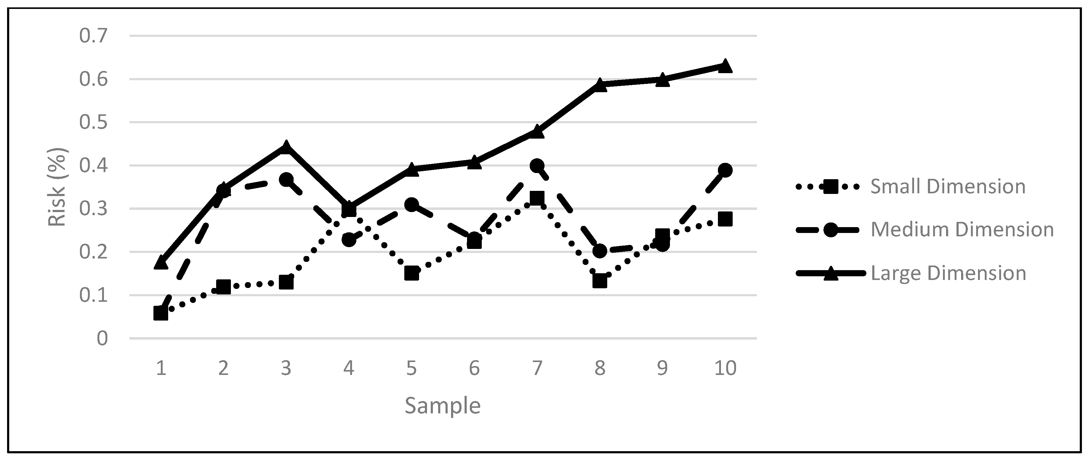
| Risk (%) | 0.058 | 0.119 | 0.13 | 0.298 | 0.151 | 0.224 | 0.324 | 0.133 | 0.237 | 0.276 |
| Samples | 1 | 2 | 3 | 4 | 5 | 6 | 7 | 8 | 9 | 10 |
| Costumer No. | 12 | 14 | 14 | 15 | 15 | 16 | 16 | 18 | 18 | 18 |
| Distributer No. | 6 | 6 | 7 | 7 | 8 | 8 | 9 | 12 | 13 | 14 |
| Cost | 1,086,833 | 1,180,532 | 1,209,745 | 1,222,165 | 1,232,836 | 1,295,891 | 1,302,785 | 1,339,529 | 1,344,999 | 1,377,401 |
| Pollution (ppm) | 1178 | 1208 | 1321 | 1342 | 1574 | 1622 | 1700 | 1765 | 1932 | 2120 |
| Time (h) | 50 | 51 | 52 | 62 | 64 | 69 | 73 | 77 | 80 | 84 |
| Risk (%) | 0.059 | 0.341 | 0.367 | 0.228 | 0.309 | 0.23 | 0.399 | 0.202 | 0.217 | 0.389 |
| Samples | 1 | 2 | 3 | 4 | 5 | 6 | 7 | 8 | 9 | 10 |
| Costumer No. | 30 | 45 | 50 | 50 | 60 | 65 | 65 | 70 | 70 | 70 |
| Distributer No. | 20 | 20 | 25 | 30 | 32 | 38 | 41 | 45 | 50 | 60 |
| Cost | 1,520,398 | 2,026,527 | 2,142,370 | 2,165,451 | 2,255,848 | 2,257,946 | 2,342,930 | 2,411,260 | 2,412,817 | 2,595,378 |
| Pollution (ppm) | 13,526 | 13,658 | 14,002 | 14,230 | 15,200 | 16,210 | 16,890 | 17,532 | 18,050 | 19,850 |
| Time (h) | 112 | 114 | 123 | 129 | 135 | 139 | 145 | 160 | 175 | 191 |
| Risk (%) | 0.177 | 0.346 | 0.443 | 0.303 | 0.391 | 0.408 | 0.479 | 0.587 | 0.599 | 0.631 |
| Distribution No. | Costumers No. | NSGA-II | MOPSO | ||||||
|---|---|---|---|---|---|---|---|---|---|
| Cost | Pollution (ppm) | Risk (%) | Time (h) | Cost | Pollution (ppm) | Risk (%) | Time (h) | ||
| 20 | 30 | 15,203,980 | 13,526 | 0.177 | 112 | 15,878,009 | 15,321 | 0.201 | 122 |
| 20 | 45 | 20,265,270 | 13,658 | 0.346 | 114 | 16,508,714 | 16,807 | 0.359 | 126 |
| 25 | 50 | 21,423,701 | 14,002 | 0.443 | 123 | 21,046,485 | 17,243 | 0.481 | 131 |
| 30 | 50 | 21,654,514 | 14,230 | 0.303 | 129 | 21,245,259 | 17,296 | 0.329 | 135 |
| 32 | 60 | 22,558,487 | 15,200 | 0.391 | 135 | 22,857,772 | 17,633 | 0.405 | 141 |
| 38 | 65 | 22,579,460 | 16,210 | 0.408 | 139 | 23,429,838 | 18,828 | 0.415 | 154 |
| 41 | 65 | 23,429,301 | 16,890 | 0.479 | 145 | 23,968,083 | 19,309 | 0.502 | 161 |
| 45 | 70 | 24,112,607 | 17,532 | 0.587 | 160 | 24,099,886 | 19,655 | 0.592 | 167 |
| 50 | 70 | 24,128,172 | 18,050 | 0.599 | 175 | 25,479,452 | 19,738 | 0.621 | 181 |
| Problem No. | 1 | 2 | 3 | 4 | 5 | 6 | 7 | 8 | 9 | 10 |
| Modified GA | 11,005,413 | 10,363,216 | 15,344,758 | 20,483,956 | 16,050,510 | 28,996,989 | 20,668,679 | 22,790,123 | 23,998,908 | 14,999,575 |
| Present Study | 11,152,821 | 10,852,524 | 15,817,908 | 20,854,215 | 16,642,758 | 29,528,210 | 21,217,931 | 23,269,604 | 24,752,042 | 15,241,798 |
| Diff. (%) | 1.34 | 4.72 | 3.08 | 1.81 | 3.69 | 1.83 | 2.66 | 2.10 | 3.14 | 1.61 |
Disclaimer/Publisher’s Note: The statements, opinions and data contained in all publications are solely those of the individual author(s) and contributor(s) and not of MDPI and/or the editor(s). MDPI and/or the editor(s) disclaim responsibility for any injury to people or property resulting from any ideas, methods, instructions or products referred to in the content. |
© 2024 by the authors. Licensee MDPI, Basel, Switzerland. This article is an open access article distributed under the terms and conditions of the Creative Commons Attribution (CC BY) license (https://creativecommons.org/licenses/by/4.0/).
Share and Cite
Pakdel, G.H.; He, Y.; Pakdel, S.H. Multi-Objective Green Closed-Loop Supply Chain Management with Bundling Strategy, Perishable Products, and Quality Deterioration. Mathematics 2024, 12, 737. https://0-doi-org.brum.beds.ac.uk/10.3390/math12050737
Pakdel GH, He Y, Pakdel SH. Multi-Objective Green Closed-Loop Supply Chain Management with Bundling Strategy, Perishable Products, and Quality Deterioration. Mathematics. 2024; 12(5):737. https://0-doi-org.brum.beds.ac.uk/10.3390/math12050737
Chicago/Turabian StylePakdel, Golnaz Hooshmand, Yong He, and Sina Hooshmand Pakdel. 2024. "Multi-Objective Green Closed-Loop Supply Chain Management with Bundling Strategy, Perishable Products, and Quality Deterioration" Mathematics 12, no. 5: 737. https://0-doi-org.brum.beds.ac.uk/10.3390/math12050737