Gray Codes Generation Algorithm and Theoretical Evaluation of Random Walks in N-Cubes

Abstract

In previous works, some of the authors have proposed a canonical form of Gray Codes (GCs) in $\mathrm{N}$-cubes (hypercubes of dimension N). This form allowed them to draw an algorithm that theoretically provides exactly all the GCs for a given dimension $\mathrm{N}$. In another work, we first have shown that any of these GC can be used to build the transition function of a Pseudorandom Number Generator (PRNG). Also, we have found a theoretical quadratic upper bound of the mixing time, i.e., the number of iterations that are required to provide a PRNG whose output is uniform. This article, extends these two previous works both practically and theoretically. On the one hand, another algorithm for generating GCs is proposed that provides an efficient generation of subsets of the entire set of GCs related to a given dimension $\mathrm{N}$. This offers a large choice of GC to be used in the construction of Choatic Iterations based PRNGs (CI-PRNGs), leading to a large class of possible PRNGs. On the other hand, the mixing time has been theoretically shown to be in $\mathrm{N}log\left(\mathrm{N}\right)$, which was anticipated in the previous article, but not proven.

1. Introduction

Random walk in the $\mathrm{N}$-cube is the process of randomly crossing edges in the hypercube of $\mathrm{N}$ dimensions. This theoretical subject has received a lot of attention in recent years [1,2,3,4,5]. The article [6] is situated in this thematic field. Indeed, it focuses on a Random Walk in a $\mathrm{N}$-cube where a balanced Hamiltonian cycle has been removed. It is worth recalling that a Hamiltonian cycle in the $\mathrm{N}$-cube is also a Gray Code (GC). To compute such kind of cycle, an algebraic solution of an undeterministic approach [7] is presented. Solving the induced system of linear equations is an easy and practicable task. However, the number of solutions found by this method is infinitely smaller than what generally exists if the approach [7] was not used.

In another work [8], we have proposed a canonical form of GCs in $\mathrm{N}$-cubes. This form allows to draw an algorithm, based on Wild’s scheme [9], that theoretically provides exactly all the GCs for a given dimension $\mathrm{N}$. However, due to the exponential growth of the number of GCs with the dimension of the $\mathrm{N}$-cube, the number of produced GCs must be specified as a boundary argument. Moreover, we have observed that the time to generate a first GC may be quite large when the dimension of the $\mathrm{N}$-cube increases.

Once a GC is produced, it can be used to build a random walk in the $\mathrm{N}$-cube based post-processing of the output of any classical PRNG [6,10,11]. This post-processing has many advantages: compared to the original PRNG which does not have a chaotic behavior according to Devaney, it first adds this property [12]. It moreover preserves the cryptographical security of the embedded PRNG [13], which may be required in a cryptographic context. Finally, it largely improves the statistical properties of the on board PRNG [14] leading to a PRNG that successfully passes not only the classical statistical tests like [15], but also the most difficult ones, namely the TestU01 [16]. In particular, it has been already presented in ([17] Chap. 5, p. 84+) that such post-processing provides a new PRNG at minimal cost which is 2.5 times faster than the PRNGs which pass the whole TestU01 [16]. Moreover, it is worth noticing that most of the classical PRNGs [18,19] do not pass the TestU01.

In such a context, the mixing time [5] corresponds to the number of steps that are required to reach any vertex with the same probability according to a given approximation tolerance $\epsilon$. In other words, it is the time until the set of vertices is $\epsilon$-close to the uniform distribution. Such a theoretical model provides information on the statistical quality of the obtained PRNG. The lower the mixing time, the more uniform the PRNG output.

We first have shown that any of the generated GC can be used to build the transition function of a Pseudorandom Number Generator (PRNG) based on random walk in the $\mathrm{N}$-cube. Then, we had found a theoretical quadratic upper bound of the mixing time.

This article is twofold as it extends these two previous works both practically and theoretically. In the first part (Section 2), we present another algorithm that can generate many GCs in a given $\mathrm{N}$-cube more efficiently than our previous algorithm. Moreover, filtering rules can be applied during the generation in order to choose codes that are especially adapted to the use in PRNG based on random walks. This leads to a very large set of possible PRNGs. In the second part (Section 4), the mixing time has been theoretically shown to be in $\mathrm{N}.{log}_2\left(\mathrm{N}\right)$, which was anticipated, but not yet proven. Then, experimental results are given and discussed in Section 5.

2. Gray Codes Generation Algorithms

In this part, we propose another algorithm that efficiently generates GCs in a given $\mathrm{N}$-cube, starting from a list of known GCs. The initial list may be reduced to a singleton.

2.1. Inverting Algorithm

Many approaches to generate GCs in a $\mathrm{N}$-cube start from one or more known codes in dimensions smaller than N [7,20,21,22,23]. However, such methods present either strong limitations over the type of cycles that can be generated, or large amount of computations that lead to non efficient generation algorithms.

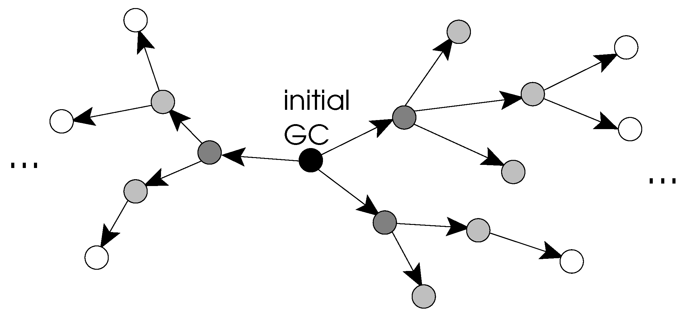
The approach we propose in this paper is quite different as it builds new Gray codes that have the same dimension as the initial known code. The principle consists in transforming one GC into another non-isomorphic GC by an adequate operation. In the sequel, we call neighbors, two GCs that are directly linked by such an operation. Hence, the key idea of the approach is to explore the space of possible GCs by generating the neighbors of the initial code and then re-applying the same strategy to the obtained codes. Therefore, in a sense, we perform a transitive closure according to the considered code transformation as depicted in Figure 1.

2.2. GC Transformation Principle

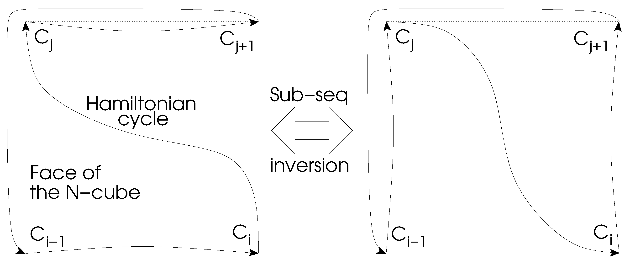
The core issue in the proposed approach above is to find a code transformation that generates another valid Gray code that is not isomorphic to the initial code. In this context, we propose what we call the inversion transformation. It consists in finding a particular sub-sequence of the initial code that can be inverted to produce another valid Gray code. If C is a GC in dimension N whose sequence of vertices is $(C_0,\dots ,C_{2^N-1})$, the problem is to find a sub-sequence $(C_i,\dots ,C_j)$ in C such that the code $(C_0,\dots ,C_{i-1},C_j,C_{j-1},\dots ,C_{i+1},C_i,C_{j+1},\dots ,C_{2^N-1})$ is also a valid GC.

We have identified conditions over the four vertices $C_{i-1}$, $C_i$, $C_j$ and $C_{j+1}$ that fulfill that constraint:

• the four vertices must be on the same face of the $\mathrm{N}$-cube, i.e., the differences between the four vertices are contained in only two dimensions of the $\mathrm{N}$-cube
• $C_i$ and $C_j$ must be diagonally opposed inside the face and, as a consequence, $C_{i-1}$ and $C_{j+1}$ are diagonally opposed too (this is equivalent to say that transitions $(C_{i-1},C_i)$ and $(C_j,C_{j+1})$ go in the same direction along their dimension)

Figure 2 illustrates the configuration providing a valid sub-sequence inversion.

Those conditions comes from the fact that in order to obtain a valid GC, the exchanges of $C_i$ and $C_j$ in the sequence must satisfies the condition of Gray codes. This implies that the number of differences between $C_{i-1}$ and $C_j$ must be only one, and this is the same for $C_i$ and $C_{j+1}$. Therefore, as $C_i$ and $C_j$ are at a Hamming distance of 1 from $C_{i-1}$ and they are different vertices (by construction of the initial GC), they must be exactly at a Hamming distance of two to each other. So, they are diagonally opposed on a same face of the $\mathrm{N}$-cube and $C_{i-1}$ is also on that face (at one of the other two corners). The same reasoning applies for $C_i$, $C_j$ and $C_{j+1}$, leading to the conclusion that $C_{j+1}$ must be at the last free corner of the same face. Therefore, it is diagonally opposed to $C_{i-1}$, leading to the configuration in Figure 2.

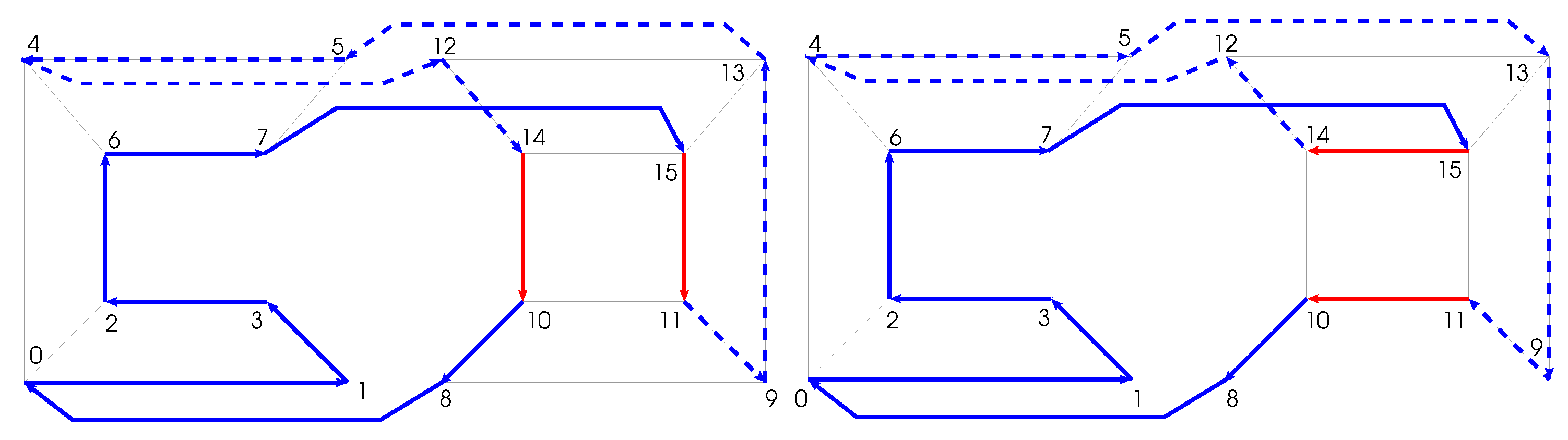
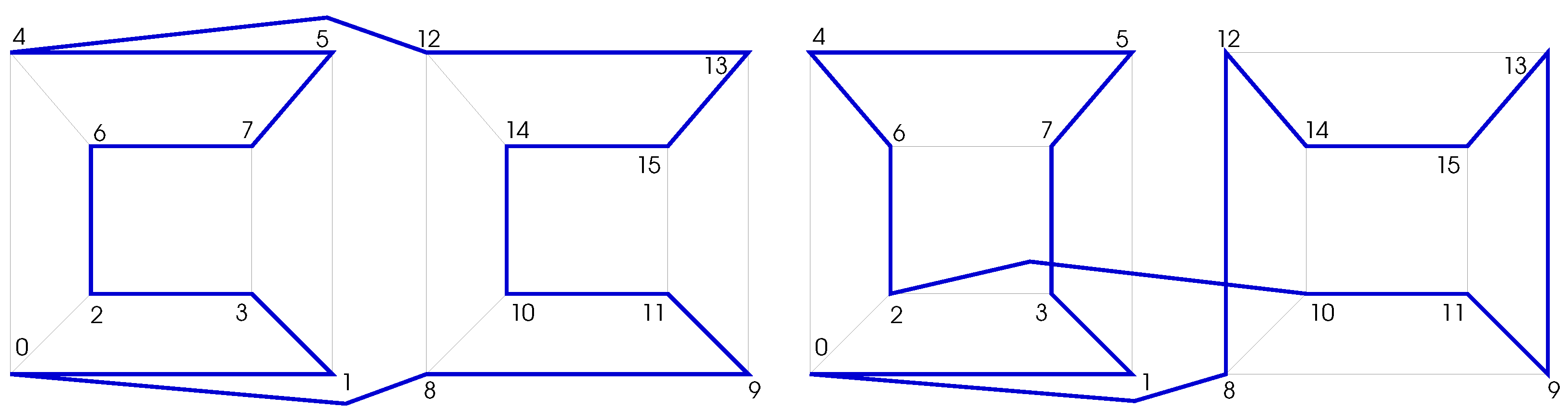
By construction, it is sure that the obtained cycle is a valid Hamiltonian cycle (Gray code in the $\mathrm{N}$-cube). Indeed, as the inversion operation is equivalent to change only some transitions of the input code, the output code contains exactly the same set of vertices as the input one. Therefore, the generated code satisfies the property of Hamiltonian cycle as it contains the total number of vertices of the considered graph. Moreover, as the Gray code property is independent of the cycle direction, the inverted sub-sequence $(C_j,\dots ,C_i)$ is still a valid part of a Gray code. Also, as explained before, the two conditions enumerated above ensure that both transitions $(C_{i-1},C_j)$ and $(C_i,C_{j+1})$, connecting the inverted sub-sequence and the unchanged part of the initial code, take place along one dimension of the $\mathrm{N}$-cube, thus satisfying the Gray code property. Therefore the generated code fulfills all the constraints of Gray codes in the $\mathrm{N}$-cube. An example of code generation in dimension 4 is given in Figure 3.

A first consequence of the sub-sequence inversion is that the codes generated from one initial code have different dimension frequencies than their source. We remind the reader that the dimension frequencies of a GC are the numbers of times each dimension is traversed by the code. The mentioned consequence comes from the fact that when inverting the sequence $(C_i,\dots ,C_j)$ in the initial code, the transitions $(C_{i-1},C_i)$ and $(C_j,C_{j+1})$ that are along the same dimension (opposite edges of the face), are respectively replaced by the transitions $(C_{i-1},C_j)$ and $(C_i,C_{j+1})$, that are along the other dimension of the face. This fact, that can be observed in Figure 2, implies that between the two cycles, the frequency of one dimension decreases by two while the frequency of another one increases by two. This is important when wanting to guide the generation towards cycles with specific properties, like the global balance of frequencies.

Another consequence is that the sub-sequence $(C_i,\dots ,C_j)$ must contain at least five vertices to go from $C_i$ to $C_j$ by traversing one dimension at a time while avoiding the vertices $C_{i-1}$ and $C_{j+1}$. This reasoning applies also to the sub-sequence $(C_{j+1},\dots ,C_{i-1})$ for the same reason. Such information can be exploited to optimize the generation algorithm.

2.3. Generation Algorithm from a Known GC

Algorithm 1 presents the sketch of the GC generation algorithm by sub-sequence inversion.

For each position in the initial sequence C, the algorithm takes the transition from this vertex as a reference and searches for any parallel transition in the sequence. By parallel transition, we mean a transition along the same dimension and in the same direction, whose vertices form a face of the $\mathrm{N}$-cube together with the vertices of the reference transition.

In this algorithm, function dimOfTransition(x,y) returns the dimension index corresponding to the transition formed by the two neighbors x and y in the $\mathrm{N}$-cube (complexity $\mathcal{O}\left(1\right)$). Also, function bitInversion(x,i) inverses the bit i of vector x ($\mathcal{O}\left(1\right)$). Function copyAndInvertSubSeq(C,a,b) returns a copy of cycle C in which the sub-sequence between indices a and b is inverted ($\mathcal{O}\left(\left|C\right|\right)$). Finally, function exclusiveInsert(C,L) inserts cycle C in list L only if C is not yet in L, and it returns the Boolean true when the insertion is performed and false otherwise ($\mathcal{O}\left({\log }_2\left(\right|L\left|\right)\right)$ thanks to the total order induced by the canonical form).

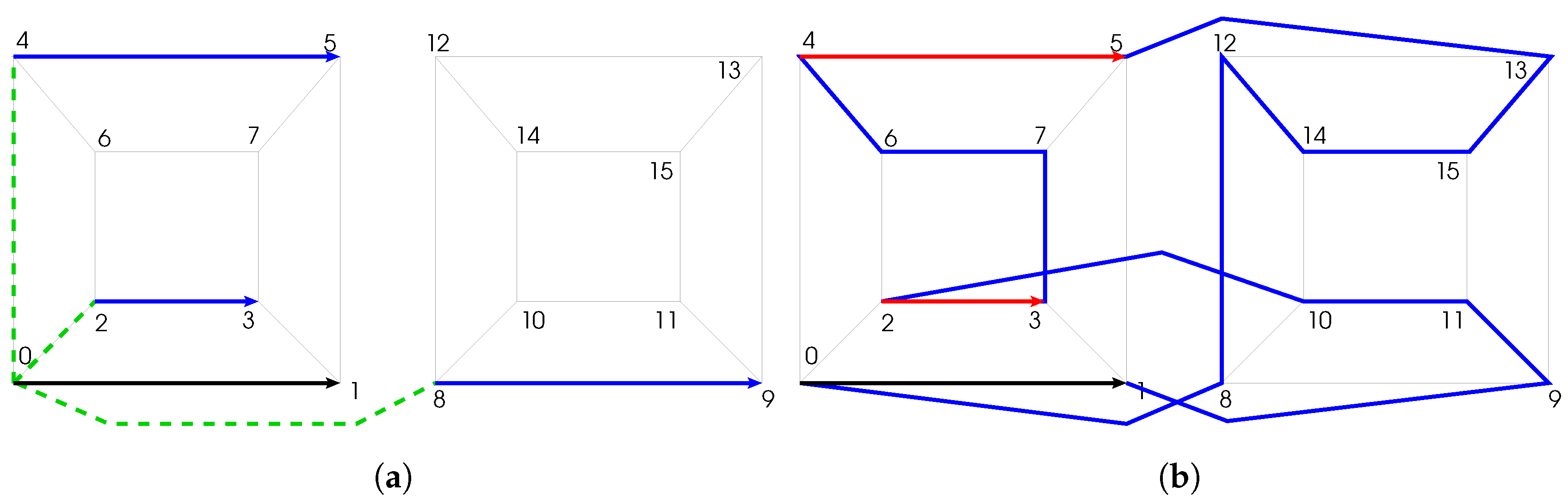
As depicted in Figure 4a, there are $N-1$ possible parallel transitions for a given transition in the $\mathrm{N}$-cube. The dotted lines exhibit the dimensions that must be parsed to get the other neighbors of the reference transition source, which are not the reference transition destination. In this particular example, the algorithm would search for sub-sequences of the form $(1,\dots ,2,3)$, $(1,\dots ,4,5)$ and $(1,\dots ,8,9)$. Each time one of these sub-sequences is found, a new GC can be produced. It is worth noticing that several sub-sequences may be valid for one reference transition, as shown in Figure 4b. In that example, the red transitions are valid parallel transitions of the black transition. Therefore, two distinct cycles can be generated by inverting either $(1,\dots ,2)$ or $(1,\dots ,4)$.

Algorithm 1: Function generateFrom(C).

To be exhaustive, and to get all the possible inversions, the algorithm applies the search for parallel transitions successively to all the transitions in the initial sequence. Also, the constraint over the minimal length of the sub-sequence to be inverted and of the unchanged part of the cycle, mentioned in the previous section, has been taken into account in the inner part of our algorithm, when searching the considered parallel transition in the cycle (boundaries of variable k). Although this does not change the overall complexity of the algorithm, it saves computations and slightly reduces the execution time. For clarity sake, the algorithm is given in its simplest form, but additional features could be added, such as a filtering over the generated cycles according to some particular properties, or a more subtle selection and guiding of the sub-sequences searches that would avoid unnecessary computations when looking for specific GCs. Also, it is recommended to sort the list $lst$ according to the canonical forms of the generated cycles, in order to perform faster exclusions or insertions.

Finally, we obtain an algorithm whose complexity to generate all the cycles that can be derived from one GC of length V is $\mathcal{O}\left(V^2.{\log }_2\left(V\right)\right)$.This corresponds to the complexity $\mathcal{O}\left(N.4^N\right)$ for the corresponding $\mathrm{N}$-cube of dimension N. Also, the memory complexity of the algorithm is $\mathcal{O}\left(c.V\right)$, where c is the number of generated cycles ($c=\left|lst\right|$). This algorithm alone is not sufficient to generate as many cycles as wanted. In fact, it is trivial to deduce a coarse upper bound of the number of possible generations from one GC of length V, which is $V.({\log }_2\left(V\right)-1)$. Thus, as explained in Section 2.1, we have designed a transitive closure algorithm that uses GC generation algorithm.

2.4. Transitive Closure Algorithm

Our transitive closure algorithm is an iterative algorithm that begins with a given set of known GCs (at least one). At the first step, each GC in the initial set is used as input to the GC generation algorithm described before. Then, the list of input GCs for the next step is rebuilt by including in it only the new cycles that have not yet been used as input GC. This clarification is important because one GC may be generated several times from different sources. So, it is necessary to maintain a list of all the GCs that have already been treated since the beginning of the process, in order to avoid duplicate work. At the next step, the GCs in the built list are used as input to the GC generation algorithm, and so on until no more GC is generated or a specific number of GCs has been reached. The overall process is detailed in Algorithm 2, in which the function generateFrom() is the one detailed in Algorithm 1.

Algorithm 2: Transitive closure generation algorithm.

Concerning the stopping criteria of the iterative process, it must include the detection that no new code has been produced at the last iteration. Also, as soon as the dimension of the $\mathrm{N}$-cube is greater than 5, the number of potential generations becomes very large and the stopping criteria must include a limitation of the number of generations. As for the previous algorithm, the lists $lst$ and $nl$ must be sorted according to the canonical forms in order to obtain fast searches and insertions.

The complexity of that algorithm is deduced by analyzing the nested loops. Although the number of iterations of the global while loop is variable, we can compute the total number of iterations of inner loops on i (line 9) and on j (line 11). This allows us to deduce an upper bound of the global complexity as the other actions performed in the while loop: the initialization of nl, the copy of nl into il and the stopping decision, take either constant or linear times (naive copy of il into nl, but optimization is possible) that are negligible compared to the total cost of the loop on i.

Concerning the loop on i, as the il list stores only the new cycles at each iteration of the closure process, we can deduce that each generated cycle is stored only once in this list, and thus is processed only once by the loop. Thus, the total number of iterations performed by this loop is equal to the total number of generated cycles (denoted by L). Inside this loop, the cost of generateFrom is $N.4^N$ as seen in the previous sub-section. The number of cycles generated by generateFrom may vary from one cycle i to another. However, an amortized complexity analysis using $\alpha$ as the average number of generations per cycle allows us to deduce that the total number of iterations performed by the inner loop in j is $\alpha .L$. This last loop is dominated by the exclusive insertions in the sorted list lst. Here also, the size of that list increases during the whole process, from 0 to L elements. In order to compute the total cost of the successive calls to exclusiveInsert(), we define S as the sum of contributions of every call with a different size of list lst : $S={\sum }_{i=0}^{L-1}{\log }_2\left(i\right)<L.{\log }_2\left(L\right)$. As there are $\alpha .L$ iterations instead of only L, this bound must be multiplied by $\alpha$. So, the total cost of loop on j is $\mathcal{O}\left(\alpha .L.{\log }_2\left(L\right)\right)$.

Finally, combining the costs of the L calls to generateFrom() and of the $\alpha .L$ iterations on j, we obtain a total cost of $\mathcal{O}\left(L.(N.4^N+\alpha .{\log }_2\left(L\right))\right)$ for the loop on i. This is clearly the dominant cost in the while loop, and thus the overall complexity of the transitive closure process. Also, the memory complexity is dominated by the list of generated cycles, leading to $\mathcal{O}\left(L.V\right)$.

Finally, it is worth noticing that for a given initial GC, the final set of GCs obtained by the transitive closure based on sub-sequence inversions may not be equal to the entire set of all possible GCs in the corresponding $\mathrm{N}$-cube, even when there is no restriction over the size of the final set. This comes from the fact that some GCs may have no valid parallel transition for any transition in the sequence, as show in Figure 5. It is worth noticing that the example on the left of this figure is a binary-reflected Gray code (BRGC) [24,25]. By construction, BRGCs do not contain any valid parallel transition, leading to no possible sub-sequence inversion. Moreover, this property is not restricted to BRGCs, as depicted in the example on the right of the figure. Indeed, such GCs with no valid parallel transition correspond to singletons in the partition of the entire set of GCs, based on the sub-sequence inversion relation. So, since the partition is composed of several connected components, the number of produced GCs will depend on the connected component of the initial GC. However, we show in Section 5 that this phenomenon is very limited in practice as the probability to get such a singleton as initial GC is very low and decreases with the dimension of the $\mathrm{N}$-cube. Moreover, in such case, it is not a problem to generate another initial GC by using any classical generation algorithm. Thus, this fact is not a significant obstacle to the generation of as many codes as wanted.

3. Using Gray Codes in Chaotic PRNGs

Full details on the use of Gray codes to build chaotic PRNGs can be found in [6,10]. For the sake of clarity, we briefly recall the main principles in this section. The chaotic PRNG can be seen as an iterative post-processing of the output of a classical PRNG of N bits (possibly with weak statistical properties) as shown in Algorithm 3. The required elements are the initial binary vector $x^0=(x_1^0,x_2^0,\dots ,x_N^0)$, a number b of iterations and an iteration function $f\left(x\right)=(f_1\left(x\right),\dots ,f_N\left(x\right))$. This function is used in the chaotic mode $F_f(x,s)$, where s is the index of the only bit of x that is updated by F, so that we have: $x^{t+1}=F_f(x^t,s_t)=(x_1^t,x_2^t,\dots ,f_s\left(x^t\right),\dots ,x_N^t)$.

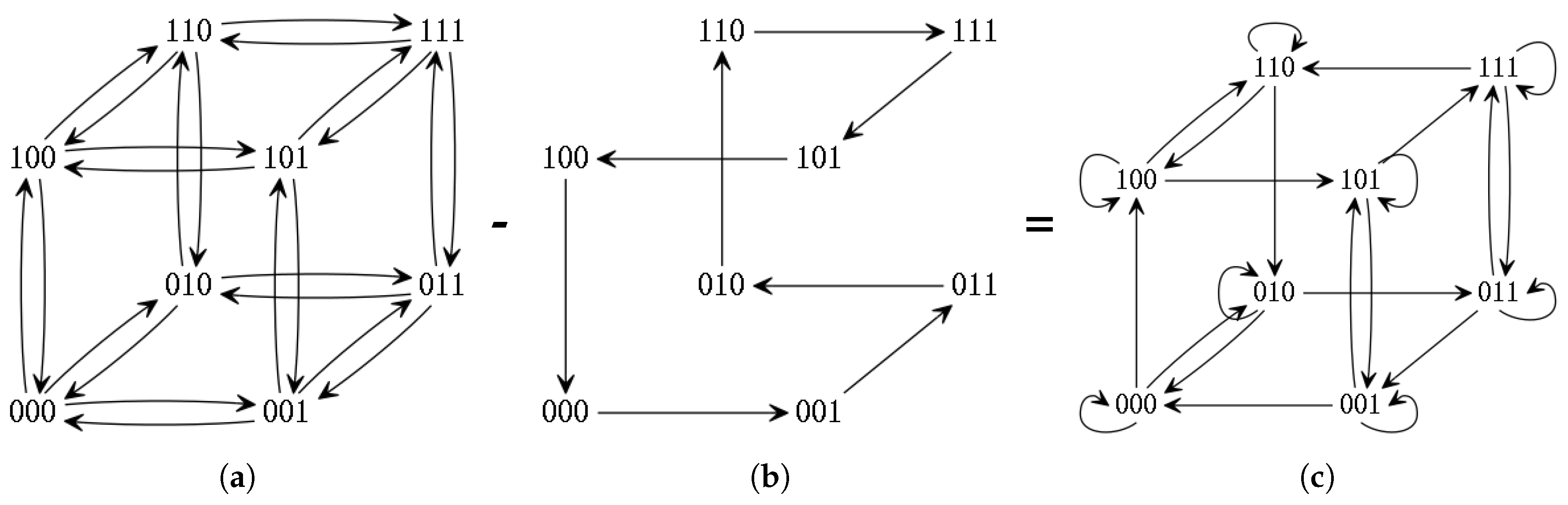
The Gray code is used in the construction of function f: for a given dimension N, we start with the complete $\mathrm{N}$-cube (Figure 6a), and we remove all the directed edges that belong to a given Gray code (Figure 6b) to obtain function f (Figure 6c). The removed edges are replaced by loop edges on every vertices.

Algorithm 3: Chaotic PRNG scheme.

Applying the function $F_f$ on the pair $(x,s)$ is equivalent to traverse the edge s from the node x in the modified $\mathrm{N}$-cube presented in Figure 6c.

4. Reducing the Mixing Time Upper Bound of Boolean Functions in the N-Cube

As mentioned in the introduction and according to the PRNG presented in the previous section, the mixing time of a Boolean function in the $\mathrm{N}$-cube provides important information about the minimal setting of the number of internal iterations of our chaotic PRNG (value b in Algorithm 3). In this section, a more accurate upper bound of this mixing time is proved by using Markov chains.

4.1. Theoretical Context

It has been proven in [10] that walking in an $\mathrm{N}$-cube where an Hamiltonian cycle has been removed induces a Markov M chain whose stationary distribution $\pi$ is the uniform one. Let us first formalize the relation between mixing time and uniform distribution.

First of all, let be given two distributions $\mu$ and $\pi$ on the same set $\mathsf{\Omega }$, the Total Variation distance ${\parallel \mu -\pi \parallel }_{\mathrm{TV}}$ is defined for by:

$${\parallel \mu -\pi \parallel }_{\mathrm{TV}}={max}_{A\subset \mathsf{\Omega }}|\mu \left(A\right)-\pi \left(A\right)|.$$

Let then $M(x,·)$ be the distribution induced by the x-th row of the Markov matrix M. If the Markov chain induced by M has a stationary distribution $\pi$, then we define

$$d\left(t\right)={max}_{x\in \mathsf{\Omega }}{\parallel M^t(x,·)-\pi \parallel }_{\mathrm{TV}}.$$

Finally, let $\epsilon$ be a positive number, the mixing time with respect to $\epsilon$ is given by

$$t_{\mathrm{mix}}\left(\epsilon \right)=min\{t\mid d\left(t\right)\le \epsilon \}.$$

It defines the smallest iteration number that is sufficient to obtain a deviation lesser than $\epsilon$ to the stationary distribution. It has been proven in ([5] Equation (4.36)) that $t_{\mathrm{mix}}\left(\epsilon \right)\le \lceil {log}_2\left({\epsilon }^{-1}\right)\rceil t_{\mathrm{mix}}\left(\frac{1}{4}\right)$. We are then left to evaluate $t_{\mathrm{mix}}\left(\frac{1}{4}\right)$.

For technical issues, rather than studying the random walk induced by the PRNG, we investigate the associated lazzy Markov chain, that is at each step, with probability $1/2$ the chain moves to the next element and with probability $1/2$ nothing is done. The mixing time of a lazzy Markov chain is about twice the mixing time of the initial chain ([26] p. 12).

Let N be a positive integer and $\mathsf{\Omega }={\{0,1\}}^N$. For $X,Y\in \mathsf{\Omega }$, we define the subset $H(X,Y)$ of $\{1,\dots ,N\}$ of indexes where X and Y differ: $H(X,Y)=\{i\mid X(i)\ne Y(i\left)\right\}$. We define the distance d on $\mathsf{\Omega }$ by $d(X,Y)=\left|H\right(X,Y\left)\right|$, that is the number of components where X and Y differ.

We also consider a Hamiltonian path on the hypercube $\mathsf{\Omega }$. More precisely, let h be a bijective function from $\mathsf{\Omega }$ to $\mathsf{\Omega }$ inducing a cyclic permutation on $\mathsf{\Omega }$ and such that for any X, $d(X,h(X\left)\right)=1$.

Since $d(X,h(X\left)\right)=1$, we denote by $f\left(X\right)$ the single index such that $X\ne h\left(X\right)$.

We consider the Markov Chain of matrix P on $\mathsf{\Omega }$ defined by:

• $P(X,X)=\frac{1}{2}+\frac{1}{2N}$,
• $P(X,Y)=\frac{1}{2N}$ if $d(X,Y)=1$ and $Y\ne h\left(X\right)$,
• $P(X,Y)=0$ otherwise.

The Markov Chain P can be defined by the following random mapping representation: $X_{n+1}=r(X_n,U,V)$ where U is a uniform random variable on $1,\dots ,N$, V a uniform random variable on $\{0,1\}$ and $r(X,U,V)=X$ if $U=f\left(X\right)$ and, otherwise, $r(X,U,V)$ is obtained from X by fixing its U-th index to V.

4.2. A Useful Random Process

The mixing time of the lazzy Markov chain will be studied in Section 4.3 using a classical coupling approach. In this section we propose a purely technical result usefull for proving some properties on this coupling.

We consider a Markov chain $\left(Z_i\right)$ on $\{0,\dots ,N\}$, of matrix K defined by:

• $\mathbb{P}(Z_{i+1}=0\mid Z_i=0)=1$,
• $\mathbb{P}(Z_{i+1}=0\mid Z_i=1)=\frac{1}{2N}$,
• $\mathbb{P}(Z_{i+1}=2\mid Z_i=1)=\frac{1}{N}$,
• $\mathbb{P}(Z_{i+1}=1\mid Z_i=1)=1-\frac{3}{2N}$,
• $\mathbb{P}(Z_{i+1}=N\mid Z_i=N)=\frac{1}{N}$ and $\mathbb{P}(Z_{i+1}=N-1\mid Z_i=N)=1-\frac{1}{N}$,
• for every $k\in \{2,\dots ,N-1\}$, $\mathbb{P}(Z_{i+1}=k-1\mid Z_i=k)=\frac{k-1}{N}$ $\begin{array}{cc}\hfill \mathrm{and}& \mathbb{P}(Z_{i+1}=k+1\mid Z_i=k)=\frac{1}{N}\hfill \\ \hfill \mathrm{and}& \mathbb{P}(Z_{i+1}=k\mid Z_i=k)=1-\frac{k}{N},\hfill \end{array}$

Let $R_d=min\{k\mid Z_k=0\mathrm{and}{Z}_0=d\}$ if it exists and ${\rho }_d=E\left[R_d\right]$.

Proposition 1.

One has ${\rho }_N\le 3N(1+e)+Nlog(N-2)$.

Proof. 

According to Theorem 1.3.5 in [27], the ${\rho }_i$ are the solution of the following system:

$$\left\{\begin{array}{cc}\hfill {\rho }_N& =1+\frac{1}{N}{\rho }_N+\frac{N-1}{N}{\rho }_{N-1}\hfill \\ \hfill {\rho }_i& =1+\frac{1}{N}{\rho }_{i+1}+\frac{i-1}{N}{\rho }_{i-1}+(1-\frac{i}{N}){\rho }_i\mathrm{for}2\le i\le N-1\hfill \\ \hfill {\rho }_1& =1+\frac{1}{2N}{\rho }_0+\frac{1}{N}{\rho }_2+(1-\frac{3}{2N}){\rho }_1\hfill \\ \hfill {\rho }_0& =0\hfill \end{array}\right.$$

This system is equivalent to:

$$\left\{\begin{array}{cc}\hfill {\rho }_N& =\frac{N}{N-1}+{\rho }_{N-1}\hfill \\ \hfill \frac{i}{N}{\rho }_i& =1+\frac{1}{N}{\rho }_{i+1}+\frac{i-1}{N}{\rho }_{i-1}\mathrm{for}2\le i\le N-1\hfill \\ \hfill \frac{3}{2N}{\rho }_1& =1+\frac{1}{N}{\rho }_2\hfill \\ \hfill {\rho }_0& =0\hfill \end{array}\right.$$

Set, for $0\le i\le N-1$, ${\alpha }_i={\rho }_{i+1}-{\rho }_i$.

Using the system, one has ${\alpha }_{N-1}=\frac{N}{N-1}$, ${\alpha }_0={\rho }_1$. Moreover, for $2\le i\le N-1$, substituting ${\rho }_{i+1}$ by ${\alpha }_i+{\rho }_i$ in the equation $\frac{i}{N}{\rho }_i=1+\frac{1}{N}{\rho }_{i+1}+\frac{i-1}{N}{\rho }_{i-1}$, one obtains that

$$\frac{i-1}{N}{\rho }_i=1+\frac{1}{N}{\alpha }_i+\frac{i-1}{N}{\rho }_{i-1}.$$

Therefore, for $2\le i\le N-1$,

$$\frac{i-1}{N}{\alpha }_{i-1}=1+\frac{1}{N}{\alpha }_i,$$

or, equivalently,

$${\alpha }_{i-1}=\frac{N}{i-1}+\frac{1}{i-1}{\alpha }_i.$$

(1)

Since ${\alpha }_{N-1}=\frac{N}{N-1}$ and using Equation (1), one has

$${\alpha }_{N-2}=\frac{N}{N-2}+\frac{N}{(N-1)(N-2)}$$

and

$${\alpha }_{N-3}=\frac{N}{N-3}+\frac{N}{(N-2)(N-3)}+\frac{N}{(N-1)(N-2)(N-3)}.$$

By a direct induction, one obtains, for $1\le k\le N-1$:

$${\alpha }_{N-k}=N\sum _{j=1}^k\prod _{\ell =0}^{j-1}\frac{1}{N-k+\ell }.$$

(2)

Consequently

$${\alpha }_{N-k}\le N\sum _{j=1}^k\prod _{\ell =0}^{j-1}\frac{1}{N-k}=N\sum _{j=1}^k\frac{1}{{(N-k)}^j}.$$

It follows that, for $1\le k\le N-2$,

$${\alpha }_{N-k}\le N\frac{1}{N-k}\frac{1-{\left(\frac{1}{N-k}\right)}^k}{1-\frac{1}{N-k}}=N\frac{1}{N-k-1}\left(1-{\left(\frac{1}{N-k}\right)}^k\right)\le \frac{N}{N-k-1}.$$

(3)

Now, for $k=N-1$, Equation (2) provides:

$${\alpha }_1=N\sum _{j=1}^{N-1}\frac{1}{j!}.$$

Therefore ${\alpha }_1\le N{\sum }_{j=0}^{N-1}\frac{1}{j!}\le Ne$, where e is the Euler number.

Consequently and using Equation (3), we have

$$\sum _{k=1}^{N-1}{\alpha }_k\le Ne+N\sum _{k=1}^{N-2}\frac{1}{N-k-1}=Ne+\sum _{k=1}^{N-2}\frac{1}{k}$$

Since the $N-2$th harmonic number ${\sum }_{k=1}^{N-2}\frac{1}{k}$ is lower than $1+log(N-2)$, we have

$$\sum _{k=1}^{N-1}{\alpha }_k\le Ne+N\left(1+log(N-2)\right).$$

Moreover, by definition of the ${\alpha }_i$’s, ${\sum }_{k=1}^{N-1}{\alpha }_k={\rho }_N-{\rho }_1$.

It follows that ${\rho }_N\le {\rho }_1+Ne+N\left(1+log(N-2)\right)$.

Since ${\rho }_2-{\rho }_1={\alpha }_1\le Ne$ and $\frac{3}{2}{\rho }_1=N+{\rho }_2$, one has $\frac{1}{2}{\rho }_1\le Ne+N$, proving that ${\rho }_1\le 2N(1+e)$. In conclusion,

$${\rho }_N\le {\rho }_1+Ne+N\left(1+log(N-2)\right)\le 3N(1+e)+Nlog(N-2),$$

which concludes the proof. ☐

4.3. A Coupling for the Markov Chain P

We now define a coupling for the lazzy Markov chain. An upper bound of the mixing time is obtained by computing the maximal expected collapsing time of the coupling ([5] Chap. 5).

Let $\left(U_n\right)$ be a sequence of i.i.d of random variables on $\{1,\dots ,N\}$, and $\left(V_n\right)$ be a sequence of i.i.d of random variables on $\{0,1\}$.

Let ${(X_n,Y_n)}_{n_{\ge }0}$ be a random sequence in $\mathsf{\Omega }$ × $\mathsf{\Omega }$ defined by:

$X_{n+1}=r(X_n,U_n,V_n)$, and $Y_{n+1}=X_{n+1}$ if $X_n=Y_n$ and, otherwise, $Y_{n+1}=r(Y_n,W_n,Z_n)$ where:

(1)

If $f\left(X\right)\in H(X,Y)$ and $f\left(Y\right)\in H(X,Y)$, then $W_n=U_n$. Moreover, if $U_n\notin H(X,Y)$ then, $Z_n=V_n$, otherwise $Z_n=1-V_n$.

(2)

If $f\left(X\right)\in H(X,Y)$ and $f\left(Y\right)\notin H(X,Y)$, then $W_n=U_n$. Moreover, if $U_n\notin H(X,Y)$ then, $Z_n=V_n$, otherwise $Z_n=1-V_n$.

(3)

If $f\left(X\right)\notin H(X,Y)$ and $f\left(Y\right)\in H(X,Y)$, then $W_n=U_n$. Moreover, if $U_n\notin H(X,Y)$ then, $Z_n=V_n$, otherwise $Z_n=1-V_n$.

(4)

If $f\left(X\right)\notin H(X,Y)$ and $f\left(Y\right)\notin H(X,Y)$, and $f\left(X\right)\ne f\left(Y\right)$. If $U_n\notin \{f\left(X\right),f\left(Y\right)\}$, then $W_n=U_n$. If $U_n=f\left(X\right)$, then $W_n=f\left(Y\right)$ and if $U_n=f\left(Y\right)$, then $W_n=f\left(X\right)$. Moreover, if $U_n\notin H(X,Y)$ then, $Z_n=V_n$, otherwise $Z_n=1-V_n$.

(5)

If $f\left(X\right)\notin H(X,Y)$ and $f\left(Y\right)\notin H(X,Y)$, and $f\left(X\right)=f\left(Y\right)$, then $W_n=U_n$. Moreover, if $U_n\notin H(X,Y)$ then, $Z_n=V_n$, otherwise $Z_n=1-V_n$.

Proposition 2.

The sequence ${(X_n,Y_n)}_{n_{\ge }0}$ is a coupling for the Markov Chain P.

Proof. 

By construction, $\left(X_n\right)$ is a Markov Chain with transition matrix P. For $\left(Y_n\right)$, it is clear that $W_n$ follows the uniform distribution on $\{1,\dots ,N\}$. ☐

Lemma 1.

Let $\left(d_n\right)$ be the sequence of integers defined by $d_n=d(X_n,Y_n)$. For any n, one has $|d_{n+1}-d_n|\le 1$. Moreover:

• If $d_n\ge 2$, then $\mathbb{P}(d_{n+1}<d_n)\ge \frac{d_n-1}{N}$.
• If $d_n\ge 2$, then $\mathbb{P}(d_{n+1}>d_n)\le \frac{1}{N}$.
• If $d_n=1$, then $\mathbb{P}(d_{n+1}=0)\ge \frac{1}{2N}$.
• If $d_n=1$, then $\mathbb{P}(d_{n+1}=2)\le \frac{1}{N}$ and $\mathbb{P}(d_{n+1}=2)\le \mathbb{P}(d_{n+1}=0)$.

Proof. 

Let $X=X_n$ and $Y=Y_n$. Assume first that $d_n\ge 2$, several cases may arise:

• If $f\left(X\right)\in H(X,Y)$ and $f\left(Y\right)\in H(X,Y)$ and $f\left(X\right)\ne f\left(Y\right)$. If $U_n\notin H(X,Y)$, then $d_{n+1}=d_n$. If $U_n\in H(X,Y)$ and $U_n\ne f\left(X\right)$ and $U_n\ne f\left(Y\right)$, then $d_{n+1}=d_n-1$. If $U_n=f\left(X\right)$ or $U_n=f\left(Y\right)$, then $d_{n+1}=d_n$ with probability $\frac{1}{2}$ and $d_{n+1}=d_n-1$ with probability $\frac{1}{2}$. It follows that, in this case, the probability that $d_{n+1}=d_n+1$ is null. The probability that $d_{n+1}=d_n-1$ is $\frac{\left|H\right(X,Y)\setminus \{f\left(X\right),f\left(Y\right)\left\}\right|}{N}+\frac{\left|\right\{f\left(X\right),f\left(Y\right)\left\}\right|}{2N}=\frac{d_n-1}{N}.$
• If $f\left(X\right)\in H(X,Y)$ and $f\left(Y\right)\in H(X,Y)$ and $f\left(X\right)=f\left(Y\right)$. If $U_n\notin H(X,Y)$, then $d_{n+1}=d_n$. If $U_n\in H(X,Y)$ and $U_n\ne f\left(X\right)$, then $d_{n+1}=d_n-1$. If $U_n=f\left(X\right)$, then $d_{n+1}=d_n$. The probability that $d_{n+1}=d_n-1$ is $\frac{\left|H\right(X,Y)\setminus \{f\left(X\right)\left\}\right|}{N}=\frac{d_n-1}{N}.$
• If $f\left(X\right)\in H(X,Y)$ and $f\left(Y\right)\notin H(X,Y)$. If $U_n\notin H(X,Y)$ and $U_n\ne f\left(Y\right)$, then $d_{n+1}=d_n$. If $U_n\in H(X,Y)$ and $U_n\ne f\left(X\right)$, then $d_{n+1}=d_n-1$. If $U_n=f\left(X\right)$, then $d_{n+1}=d_n$ with probability $\frac{1}{2}$ and $d_{n+1}=d_n-1$ with probability $\frac{1}{2}$. If $U_n=f\left(Y\right)$, then $d_{n+1}=d_n+1$ with probability $\frac{1}{2}$ and $d_{n+1}=d_n$ with probability $\frac{1}{2}$. It follows that the probability that $d_{n+1}=d_n+1$ is $\frac{1}{2N}$, and the probability that $d_{n+1}=d_n-1$ is $\frac{\left|H\right(X,Y)\setminus \{f\left(X\right)\left\}\right|}{N}+\frac{\left|\right\{f\left(X\right)\left\}\right|}{2N}\ge \frac{d_n-1}{N}$.
• If $f\left(X\right)\notin H(X,Y)$ and $f\left(Y\right)\in H(X,Y)$. This is a dual case of the previous one with similar calculus, switching $f\left(X\right)$ and $f\left(Y\right)$.
• If $f\left(X\right)\notin H(X,Y)$ and $f\left(Y\right)\notin H(X,Y)$, and $f\left(X\right)\ne f\left(Y\right)$. If $U_n\notin H(X,Y)\setminus \{f\left(X\right),f\left(Y\right)\}$, then $d_{n+1}=d_n$. If $U_n\in H(X,Y)$, then $d_{n+1}=d_n-1$. If $U_n=f\left(X\right)$, then $d_{n+1}=d_n$ with probability $\frac{1}{2}$ and $d_{n+1}=d_n+1$ with probability $\frac{1}{2}$. Similarly, If $U_n=f\left(Y\right)$, then $d_{n+1}=d_n$ with probability $\frac{1}{2}$ and $d_{n+1}=d_n+1$ with probability $\frac{1}{2}$. Consequently, the probability that $d_{n+1}=d_n+1$ is $\frac{1}{2N}+\frac{1}{2N}=\frac{1}{N}$. Moreover the probability that $d_{n+1}=d_n-1$ is $\frac{\left|H\right(X,Y\left)\right|}{N}=\frac{d_n}{N}\ge \frac{d_n-1}{N}$.
• If $f\left(X\right)\notin H(X,Y)$ and $f\left(Y\right)\notin H(X,Y)$, and $f\left(X\right)=f\left(Y\right)$. If $U_n\in H(X,Y)$, then $d_{n+1}=d_n-1$. If $U_n\notin H(X,Y)$, then $d_{n+1}=d_n$. It follows that the probability that $d_{n+1}=d_n+1$ is null and the probability that $d_{n+1}=d_n-1$ id $\frac{\left|H\right(X,Y\left)\right|}{N}=\frac{d_n}{N}\ge \frac{d_n-1}{N}.$

Now assume that $d_n=1$. By definition, $\left|H\right(X,Y\left)\right|=1$. The following cases arise:

• If $f\left(X\right)=f\left(Y\right)$. Since f is induced by an Hamiltonian cycle and $N\ge 2$, we cannot have $H(X,Y)=\left\{f\right(X\left)\right\}$. If $U_n\notin H(X,Y)$, then $d_{n+1}=d_n$. If $U_n\in H(X,Y)$, $d_{n+1}=d_n-1$. Therefore, the probability that $d_{n+1}=d_n+1$ is null and the probability that $d_{n+1}=d_n-1=0$ is $\frac{1}{N}$.
• If $f\left(X\right)\ne f\left(Y\right)$ and $H(X,Y)=\left\{f\right(X\left)\right\}$. If $U_n\ne f\left(X\right)$ and $U_n\ne f\left(Y\right)$, then $d_{n+1}=d_n$. If $U_n=f\left(X\right)$, then $d_{n+1}=0$ with probability $\frac{1}{2}$ and $d_{n+1}=d_n=1$ with probability $\frac{1}{2}$. If $U_n=f\left(Y\right)$, then $d_{n+1}=d_n+1=2$ with probability $\frac{1}{2}$ and $d_{n+1}=d_n=1$ with probability $\frac{1}{2}$. Therefore, the probability that $d_{n+1}=2$ is $\frac{1}{2N}$ and the probability that $d_{n+1}=0=\frac{1}{2N}$.
• If $f\left(X\right)\ne f\left(Y\right)$ and $H(X,Y)=\left\{f\right(Y\left)\right\}$. It a dual case of the previous one. The probability that $d_{n+1}=2$ is $\frac{1}{2N}$ and the probability that $d_{n+1}=0=\frac{1}{2N}$.
• If $f\left(X\right)\ne f\left(Y\right)$ and $H(X,Y)\cap \left\{f\right(X),f(Y\left)\right\}=\varnothing$. If $U_n\ne f\left(X\right)$ and $U_n\ne f\left(Y\right)$, then $d_{n+1}=d_n$. If $U_n=f\left(X\right)$ (resp. $f\left(Y\right)$), then $d_{n+1}=d_n+1=2$ with probability $\frac{1}{2}$ and $d_{n+1}=d_n=1$ with probability $\frac{1}{2}$. Therefore, the probability that $d_{n+1}=2$ is $\frac{1}{N}$ and the probability that $d_{n+1}=0=\frac{1}{N}$.
   ☐

Let $T(X,Y)$ the random variable of the first coupling time of $(X_n,Y_n)$, with $X_0=X$ and $Y_0=Y$, i.e., $T(X,Y)=k$ if $X_k=Y_k$ and $X_i\ne Y_i$ for $i<k$. Let $\tau (X,Y)=E\left[T\right(X,Y\left)\right]$ and $\tau =ma{x}_{X,Y}\tau (X,Y)$.

Proposition 3.

One has $\tau \le {\rho }_N$.

Proof. 

By Proposition 1 and Lemma 1. ☐

By classical results on coupling ([5] Corollary 5.3) and Markov inequality, one has $d\left(t\right)\le \frac{\tau }{t}$. Thus, $t_{\mathrm{mix}}(1/4)\le 4\tau$ and finally

$$t_{\mathrm{mix}}\left(\epsilon \right)\le \lceil {log}_2\left({\epsilon }^{-1}\right)\rceil \left(12N(1+e)+4Nlog(N-2)\right).$$

(4)

5. Experiments

In this section is presented a set of different experiments in relation to the GC generation algorithm and the mixing time.

5.1. Performance of Gray Codes Generation Algorithms

The first series of experiments is devoted to the performance of the GC generation algorithm. The execution times shown below have been obtained on a desktop machine with two Intel(R) Xeon(R) CPU E5-2640 v2 @ 2.00GHz containing eight cores each and 128GB RAM. The OS is Linux Debian 3.16.43 and the program is written in C/C++ and uses the OpenMP multi-threading library. Indeed, the implementation of our algorithm is multi-threaded and takes advantage of the available cores in the machine. This reduces the execution times but does not change the overall complexity of the algorithm. Also, different compilers have been tested (GCC, Intel, PGI) and although slight variations may be observed, the executions times are quite similar. Times given below are averages of a series of executions.

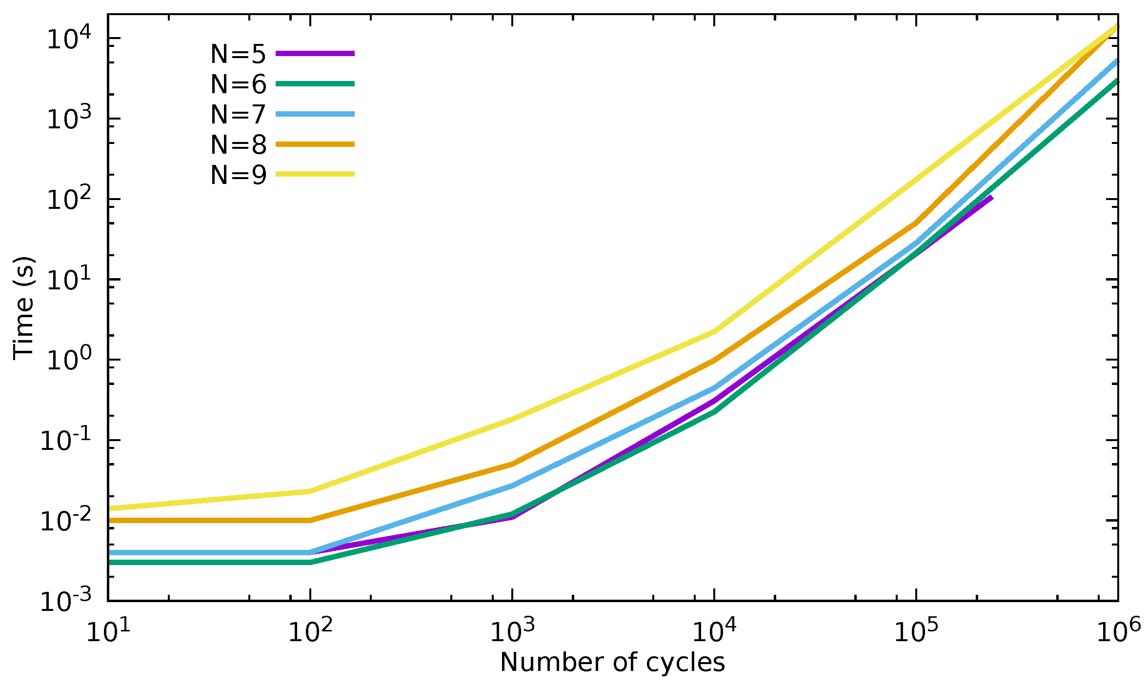
Two series of results are presented that exhibits the behavior of the performance our algorithm either in function of the dimension of the $\mathrm{N}$-cube or in function of the number of GCs to generate.

In

Table 1. Generation times of 100,000 Gray Codes (GCs) in function of the dimension of the $\mathrm{N}$-cube.

dim	5	6	7	8	9	10
time (s)	19.61	19.93	28.17	53.60	174.43	332.29

are provided the execution times for generating 100,000 cycles in $\mathrm{N}$-cubes of dimensions 5 to 10. Smaller dimensions have too few GCs to get representative times (only one GC in dimensions 2 and 3 and 9 in dimension 4). As expected, the execution time increases with the dimension. However, the progression is much slower than the theoretical complexity obtained in Section 2.4. This means that this upper bound of complexity is largely overestimated. Indeed, many iterations in the inner loop of the generation algorithm are not performed, since it stops as soon as a parallel transition has been found. This is not taken into account in the current estimation of the complexity but it will deserve a deeper study to get a more accurate expression.

The execution times for generating different amounts of GCs in dimensions between 5 and 9 are given in Figure 7. We observe similar behaviors for all dimensions with a sharp increase of the execution time with the number of GCs. This mainly comes from the fact that in the closure algorithm, GCs may be generated as much times as their number of neighbors according to the sub-sequence inversion relation. Moreover, this number of duplicate generations increases with the size of the input list, which itself increases with the size of the generated set. This is why we observe such an exponential increase. A strategy to avoid such duplicates during the transitive closure will be investigated in future works. Nonetheless, the absolute performance of the current version is rather efficient when considering that the production of several thousands of GCs takes less than one minute.

To conclude this part on the performance of the generation process, a first multi-threaded implementation has been tested, which provides gains between 16% and 90% depending on the number of generated cycles and the dimension of the $\mathrm{N}$-cube. However, this first implementation is far from being optimal and additional development effort is planed as a future work.

5.2. Statistical Study of the Generation Algorithm

This second series of experiments aims at analyzing the impact of the presence of isolated GCs according to the sub-sequence inversion relation, as mentioned in Section 2.4.

Table 2. Percentages of isolated GCs in the partition of the set of GCs.

dim	2	3	4	5
nb of isolated GCs	1	1	3	740
total nb of GCs	1	1	9	237,675
ratio of isolated (%)	100	100	33.3	0.3

gives the percentages of isolated GCs in dimensions 2 to 5 of $\mathrm{N}$-cubes. It is not possible to get exact percentages for greater dimensions due to the exponential increase of the number of GCs. However, it is interesting to see that the ratio of isolated GCs drastically decreases when the dimension of the $\mathrm{N}$-cube increases. It can be proved that this tendency continues with greater dimensions. This comes from the condition that a GC must satisfy to be isolated, i.e., to generate no other GC by the inversion algorithm. The condition is that it must not have any valid parallel transitions in its entire sequence. However, for one transition, the number of possible parallel transitions is directly linked to the dimension of the $\mathrm{N}$-cube. Moreover, the number of transitions in a sequence exponentially increases with the dimension of the $\mathrm{N}$-cube. Therefore, the probability of having at least one valid parallel transition in the entire sequence exponentially increases with the dimension of the $\mathrm{N}$-cube. Indeed, the constraint to satisfy becomes stronger and stronger as the dimension increases. Thus, it comes that the probability that a GC is isolated, i.e., is a singleton in the partition of the set of GCs, exponentially decreases when the dimension of the $\mathrm{N}$-cube increases. Finally, this implies that the constraint over the choice of GCs as input to the closure algorithm is very weak, as most GCs will lead to the generation of other GCs.

5.3. Discussion over the Mixing Time Distributions in Dimensions 5 and 8

First of all, the mixing time is bounded by $\lceil log\left({\epsilon }^{-1}\right)\rceil {\rho }_N$ and thus, thanks to Proposition 1 by $\lceil log\left({\epsilon }^{-1}\right)\rceil 3N(1+e)+Nlog(N-2)$.

For instance, for $\epsilon ={10}^{-6}$, $N=5$, or $N=8$ these bounds are respectively equal to 319 and 550. In the same context, i.e., $\epsilon ={10}^{-6}$, we practically observe that the largest mixing time for all the Markov chains when $N=5$ is equal to 42. It can be thus notably deduced that theoretical bound provided in Proposition 1 is notably much larger than the practical one.

6. Conclusions

Practical and theoretical contributions have been presented in this paper, respectively related to the field of Gray codes generation and mixing time of Boolean functions in dimension N.

Concerning Gray codes generation, an algorithm based on sub-sequence inversion has been designed and implemented. It starts from one known GC and it produces new GCs of the same dimension. It has been explained why the number of generations strongly depends on the configuration of the input GC. Then, as the upper bound of the number of generations from a single GC is limited, a transitive closure algorithm has been proposed too, that can generate very large subsets of the entire set of GCs in a given $\mathrm{N}$-cube. Such algorithms are essential to study the Gray Code properties that may present a particular interest for use in a chaotic PRNG based on random walks or jumps in a $\mathrm{N}$-cube.

Experiments have shown that our algorithm can produce several thousands of GCs in time of the order of the minute. Also, it has been shown that for a given dimension of $\mathrm{N}$-cube, the number of isolated GCs, i.e., the codes that do not allow any sub-sequence inversion, is a negligible part of the total number of GCs. Moreover, this ratio decreases when the dimension increases. Therefore, the probability that our algorithm does not produce any new GC from a given input, is very small.

Concerning the mixing time of Boolean functions in the $\mathrm{N}$-cube, the complete proof of an upper bound in $\mathcal{O}\left(N.{\log }_2\left(N\right)\right)$ has been given. This is the most accurate upper bound that has been proved to this day.

Such result is useful to limit significantly the number of iterations when computing mixing times of boolean functions in the $\mathrm{N}$-cube. This is of particular interest when looking for such functions that would be adequate for the use in a CI-PRNG, i.e., functions with minimal mixing time, among a large number of candidates.

In future works, we plan to address the potential algorithmic enhancements mentioned in the experiments, and to perform deep statistical analyzes of Gray codes according to the mixing times of their respective Boolean functions in the $\mathrm{N}$-cube as well as other features. This will help to identify the particular properties of GCs that could be used to find the codes best suited to the use in PRNGs. The results presented in this paper directly contribute to make such statistical analyzes possible.

References

- Lovász, L. Random walks on graphs. In Combinatorics, Paul Erdos Is Eighty; János Bolyai Mathematical Society: Budapest, Hungary, 1993; Volume 2, pp. 1–46. [Google Scholar]
- Diaconis, P.; Graham, R.L.; Morrison, J.A. Asymptotic analysis of a random walk on a hypercube with many dimensions. Random Struct. Algorithms 1990, 1, 51–72. [Google Scholar] [CrossRef]
- Lawler, G.F.; Limic, V. Random Walk: A Modern Introduction; Cambridge University Press: Cambridge, UK, 2010; Volume 123. [Google Scholar]
- Scoppola, B. Exact solution for a class of random walk on the hypercube. J. Stat. Phys. 2011, 143, 413–419. [Google Scholar] [CrossRef]
- Levin, D.A.; Peres, Y. Markov Chains and Mixing Times; American Mathematical Soc.: Providence, RI, USA, 2017; Volume 107. [Google Scholar]
- Contassot-Vivier, S.; Couchot, J.F.; Guyeux, C.; Héam, P.C. Random Walk in a N-Cube Without Hamiltonian Cycle to Chaotic Pseudorandom Number Generation: Theoretical and Practical Considerations. Int. J. Bifurcation Chaos 2017, 27, 18. [Google Scholar] [CrossRef]
- Suparta, I.; Zanten, A.V. Totally balanced and exponentially balanced Gray codes. Discrete Anal. Oper. Res. 2004, 11, 81–98. (In Russia) [Google Scholar]
- Contassot-Vivier, S.; Couchot, J.F. Canonical Form of Gray Codes in N-cubes. In Cellular Automata and Discrete Complex Systems, Proceedings of the 23th International Workshop on Cellular Automata and Discrete Complex Systems (AUTOMATA), Milan, Italy, 7–9 June 2017; Part 2: Regular Papers; Dennunzio, A., Formenti, E., Manzoni, L., Porreca, A.E., Eds.; Springer International Publishing: Milan, Italy, 2017; Volume LNCS-10248, pp. 68–80. [Google Scholar]
- Wild, M. Generating all cycles, chordless cycles, and Hamiltonian cycles with the principle of exclusion. J. Discrete Algorithms 2008, 6, 93–102. [Google Scholar] [CrossRef]
- Couchot, J.; Héam, P.; Guyeux, C.; Wang, Q.; Bahi, J.M. Pseudorandom Number Generators with Balanced Gray Codes. In Proceedings of the 11th International Conference on Security and Cryptography SECRYPT, Vienna, Austria, 28–30 August 2014; pp. 469–475. [Google Scholar]
- Bakiri, M.; Couchot, J.; Guyeux, C. CIPRNG: A VLSI Family of Chaotic Iterations Post-Processings for F2-Linear Pseudorandom Number Generation Based on Zynq MPSoC. IEEE Trans. Circuits Syst. 2018, 65, 1628–1641. [Google Scholar] [CrossRef]
- Bahi, J.M.; Couchot, J.F.; Guyeux, C.; Richard, A. On the Link between Strongly Connected Iteration Graphs and Chaotic Boolean Discrete-Time Dynamical Systems. In Fundamentals of Computation Theory; Owe, O., Steffen, M., Telle, J.A., Eds.; Springer Berlin Heidelberg: Berlin, Heidelberg, Germany, 2011; pp. 126–137. [Google Scholar]
- Guyeux, C.; Couturier, R.; Héam, P.; Bahi, J.M. Efficient and cryptographically secure generation of chaotic pseudorandom numbers on GPU. J. Supercomput. 2015, 71, 3877–3903. [Google Scholar] [CrossRef] [Green Version]
- Bakiri, M.; Couchot, J.; Guyeux, C. FPGA Implementation of F2-Linear Pseudorandom Number Generators based on Zynq MPSoC: A Chaotic Iterations Post Processing Case Study. In Proceedings of the 13th International Joint Conference on e-Business and Telecommunications (ICETE 2016): SECRYPT, Lisbon, Portugal, 26–28 July 2016; Callegari, C., van Sinderen, M., Sarigiannidis, P.G., Samarati, P., Cabello, E., Lorenz, P., Obaidat, M.S., Eds.; SciTePress: Setúbal, Portugal, 2016; Volume 4, pp. 302–309. [Google Scholar]
- Marsaglia, G. DIEHARD: A Battery of Tests of Randomness. Available online: https://tams.informatik.uni-hamburg.de/paper/2001/SA_Witt_Hartmann/cdrom/Internetseiten/stat.fsu.edu/diehard.html.
- L’Ecuyer, P.; Simard, R. TestU01: A C Library for Empirical Testing of Random Number Generators. ACM Trans. Math. Softw. 2007, 33, 22. [Google Scholar]
- Bakiri, M. Hardware Implementation of Pseudo Random Number Generator Based on Chaotic Iterations. Ph.D Thesis, Université Bourgogne Franch-Comté, Belfort, France, 2018. [Google Scholar]
- L’Ecuyer, P. Handbook of Computational Statistics; Springer-Verlag: Berlin, Germany, 2012; Chapter Random Number Generation; pp. 35–71. [Google Scholar]
- L’Ecuyer, P. History of uniform random number generation. In Proceedings of the WSC 2017-Winter Simulation Conference, Las Vegas, NV, USA, 3–6 December 2017; pp. 202–230. [Google Scholar]
- Robinson, J.P.; Cohn, M. Counting Sequences. IEEE Trans. Comput. 1981, 30, 17–23. [Google Scholar] [CrossRef]
- Bhat, G.S.; Savage, C.D. Balanced Gray Codes. Electr. J. Comb. 1996, 3, 25. [Google Scholar]
- Suparta, I.; Zanten, A.V. A construction of Gray codes inducing complete graphs. Discrete Math. 2008, 308, 4124–4132. [Google Scholar] [CrossRef]
- Bykov, I.S. On locally balanced gray codes. J. Appl. Ind. Math. 2016, 10, 78–85. [Google Scholar] [CrossRef]
- Conder, M.D.E. Explicit definition of the binary reflected Gray codes. Discrete Math. 1999, 195, 245–249. [Google Scholar] [CrossRef]
- Bunder, M.W.; Tognetti, K.P.; Wheeler, G.E. On binary reflected Gray codes and functions. Discrete Math. 2008, 308, 1690–1700. [Google Scholar] [CrossRef]
- Berestycki, N. Mixing Times of Markov Chains: Techniques and Examples. Graduate course at cambridge. University of Cambridge: Cambridge, UK, 2016. Available online: http://www.statslab.cam.ac.uk/ beresty/teach/Mixing/mixing3.pdf.
- Norris, J.R. Markov Chains; Cambridge University Press: Cambridge, UK, 1998; ISBN 9780521633963. [Google Scholar]
Figure 1.
Transitive exploration of the space of Gray Codes (GCs) from the initial black code. Each dot represents one GC. The color gets lighter at each additional transform.
Figure 2.
Inversion of sub-sequence inside a face of the -cube (dotted square).
Figure 3.
Inversion of sub-sequence (dotted line) on face (10, 11, 14, 15) in the 4-cube.
Figure 4.
Examples of possible and valid parallel transitions in the 4-cube. (a) Possible parallel transitions (blue) for a reference transition (black); (b) Two valid parallel transitions (red) for the reference transition (black) in the blue cycle.
Figure 5.
Cycles in the 4-cube with no valid parallel transition.
Figure 6.
Construction of function f in dimension 3. (a) Original 3-cube; (b) A Gray code; (c) Function f.
Figure 7.
Exec times (s) in function of the number of generated GCs for different dimensions of -cube.