A New Operational Matrix of Fractional Derivatives to Solve Systems of Fractional Differential Equations via Legendre Wavelets


1
Department of Mathematical Engineering, Yildiz Technical University, Istanbul 34200, Turkey
2
Yildiz Technical University, Istanbul 34200, Turkey
*
Author to whom correspondence should be addressed.
Mathematics 2018, 6(11), 238; https://0-doi-org.brum.beds.ac.uk/10.3390/math6110238
Submission received: 2 October 2018
/
Revised: 29 October 2018
/
Accepted: 31 October 2018
/
Published: 5 November 2018
(This article belongs to the Special Issue Fractional-Order Integral and Derivative Operators and Their Applications)
Abstract
:This paper introduces a new numerical approach to solving a system of fractional differential equations (FDEs) using the Legendre wavelet operational matrix method (LWOMM). We first formulated the operational matrix of fractional derivatives in some special conditions using some notable characteristics of Legendre wavelets and shifted Legendre polynomials. Then, the system of fractional differential equations was transformed into a system of algebraic equations by using these operational matrices. At the end of this paper, several examples are presented to illustrate the effectivity and correctness of the proposed approach. Comparing the methodology with several recognized methods demonstrates that the advantages of the Legendre wavelet operational matrix method are its accuracy and the understandability of the calculations.
1. Introduction
Differential and integral operators are the basis of mathematical models, and they are also used as a means of understanding the working principles of natural and artificial systems. Therefore, differential and integral equations are of great importance both theoretically and practically. Such equations have a wide range of applications, including in the physical sciences (such as in physics and engineering) as well as in social science. Systems of differential equations, as differential equations, are often used in issues such as theories of elasticity, dynamics, fluid mechanics, oscillation, and quantum dynamics.
Interest in differential and integral operators has led to the exploration of fractional differential and integral operators by examining these issues further in depth. Owing to a question, the origin of fractional calculus arose in a message from Leibniz to L’Hôpital in 1695. Fractional calculus has received attention in recent years due to its ability to simplify numerous physical, engineering, and economics phenomena such as the fluid dynamic traffic model, damping laws, continuum and statistical mechanics, diffusion processes, solid mechanics, control theory, colored noise, viscoelasticity, electrochemistry, and electromagnetism, among others.
Because a variety of solutions of fractional differential equations (FDEs) cannot be found analytically, numerical and approximate methods are needed. There are a lot of techniques that have been studied by many researchers in solving FDEs and the system of such equations numerically. Some of these techniques are the Adomian decomposition method presented by Song and Wang [1], the collocation method, the improved operational matrix method [2,3,4], the perturbation iteration method introduced by Şenol and Dolapçı [5], the computational matrix method illustrated by Khader et al. [6], the differential transform method demonstrated by Ertürk and Momani [7], the variational iteration method, the Laplace transform method given by Gupta et al. [8], and the fractional complex transform method studied by Ghazanfari and Ghazanfari [9], among others. Kilbas et al. [10] inclusively examined fractional differential and fractional integro-differential equations. In addition, numerical solutions of FDEs and the system of such equations have been presented using the Legendre polynomial operational matrix method [11], Bernstein operational matrix method [12], Genocchi operational matrix method [13], Jacobi operational matrix method [14], Chebyshev wavelet operational matrix method [15], polynomial least squares method (PLSM) [16], Legendre wavelet-like operational matrix method (LWPT) [17], and the Genocchi wavelet-like operational matrix method [18].
This paper focuses on the numerical analysis of a system of fractional order differential equations using the Legendre wavelet operational matrix method. The most important advantage of the proposed method is that it presents an understandable procedure to reduce FDEs and the system of such equations to a system of algebraic equations. First, we begin by presenting some basic definitions and fundamental relations in Section 2 and Section 3, respectively. Then, in Section 4, the operational matrix of the fractional derivate is natively formulated to linear and nonlinear systems of fractional differential equations. Section 5 presents five illustrative examples that were tested with the introduced method. Finally, the last section includes the conclusions.
2. Basic Definitions
The Liouville_Caputo fractional_order derivative, shifted Legendre polynomials, and Legendre wavelets are defined below [19,20].
Definition 1.
The Liouville_Caputo fractional derivative of is defined as [19]
Some characteristics of the Liouville_Caputo fractional derivative are as follows:
where is a constant. In addition, there is
in which and respectively imply that the largest integer is less than or equal to , and the smallest integer is greater than or equal to .
The Liouville_Caputo fractional order derivative is a linear operation of the integer order derivative
where and are constant.
Definition 2.
Definition 3.
Let imply the shifted Legendre polynomials of order . Then can be formulated as [21]
and the orthogonality condition is
Definition 4.
3. Fundamental Relations
Saadatmandi and Dehghan [11] derived the operational matrix of a fractional derivative by using shifted Legendre polynomials. In this section, we show how we derived the Legendre wavelet operational matrix of fractional derivatives in some special conditions by drawing from Saadatmandi and Dehghan [11]. Additionally, the theorem and corollary related to the Legendre wavelet operational matrix of derivatives illustrated by Mohammadi [21] are cited here as follows.
Theorem 1.
Corollary 1.
Using Equation (12), the operational matrix for the derivative can be stated as [21]
where is the power of matrix.
Lemma 1.
Let be the Legendre wavelets vector introduced in Equation (8). Assuming that , then
Proof.
The desired result can be obtained by using Equations (2) and (4) in Equation (8). □
Theorem 2.
Let be the Legendre wavelets vector introduced in Equation (8). Supposing that and , then
where is the operational matrix of the fractional derivative of the order in the Liouville_Caputo sense and can be stated as
where is written as
Consider in that the first rows are all zero.
Proof.
Presume that is the element of the vector introduced in Equation (11), where . Then can be stated as
Accepting that , and by using the shifted Legendre polynomial, we obtain
If we use Equations (3), (4), and (21), then we have
Approximating by terms of the Legendre wavelets, then we obtain
where
Utilizing Equations (22) and (24), we get
in which is presented in Equation (19). In addition, if we use Lemma 1, then we can write
Combining Equations (25) and (27), the result can be obtained. □
4. Solving Systems of Fractional Order Differential Equations
In this section, the Legendre wavelet operational matrix method was implemented to obtain the numerical solution of the system of fractional order differential equations. Consider a system of fractional differential equations as follows:
where is a linear/nonlinear function of is the derivative of with the order of in the Liouville–Caputo sense and , and they are subjected to the initial conditions
First of all, approximating and , we obtain
where is an unknown vector and is the vector introduced in Equation (8). If we utilize Equation (17), then we have
Substituting Equations (29) and (30) into Equation (27), we obtain
If is a linear function of then we produce linear equations by implementing
Also, by substituting the initial conditions in Equation (28) into Equation (30), then we obtain
A set of linear equations is generated by combining Equations (32) and (33). The solution of these linear equations can be obtained for unknown coefficients of the vector . Consequently, , introduced in Equation (27), can be computed.
If is a nonlinear function of then we first compute at points and, for a better result, use the first roots of shifted Legendre . Then these equations, collectively with Equation (33), produce nonlinear equations. The solution of these nonlinear equations can be obtained by employing Newton’s iterative method. Consequently, , introduced in Equation (27), can be computed.
5. Illustrative Examples
In this section, to show the applicability and powerfulness of the introduced method, we present the solutions to five linear and nonlinear systems of fractional order differential equations.
Example 1.
We first considered the following linear system of fractional differential equations [7,8]:
subject to
The exact solution of this system when is known to be
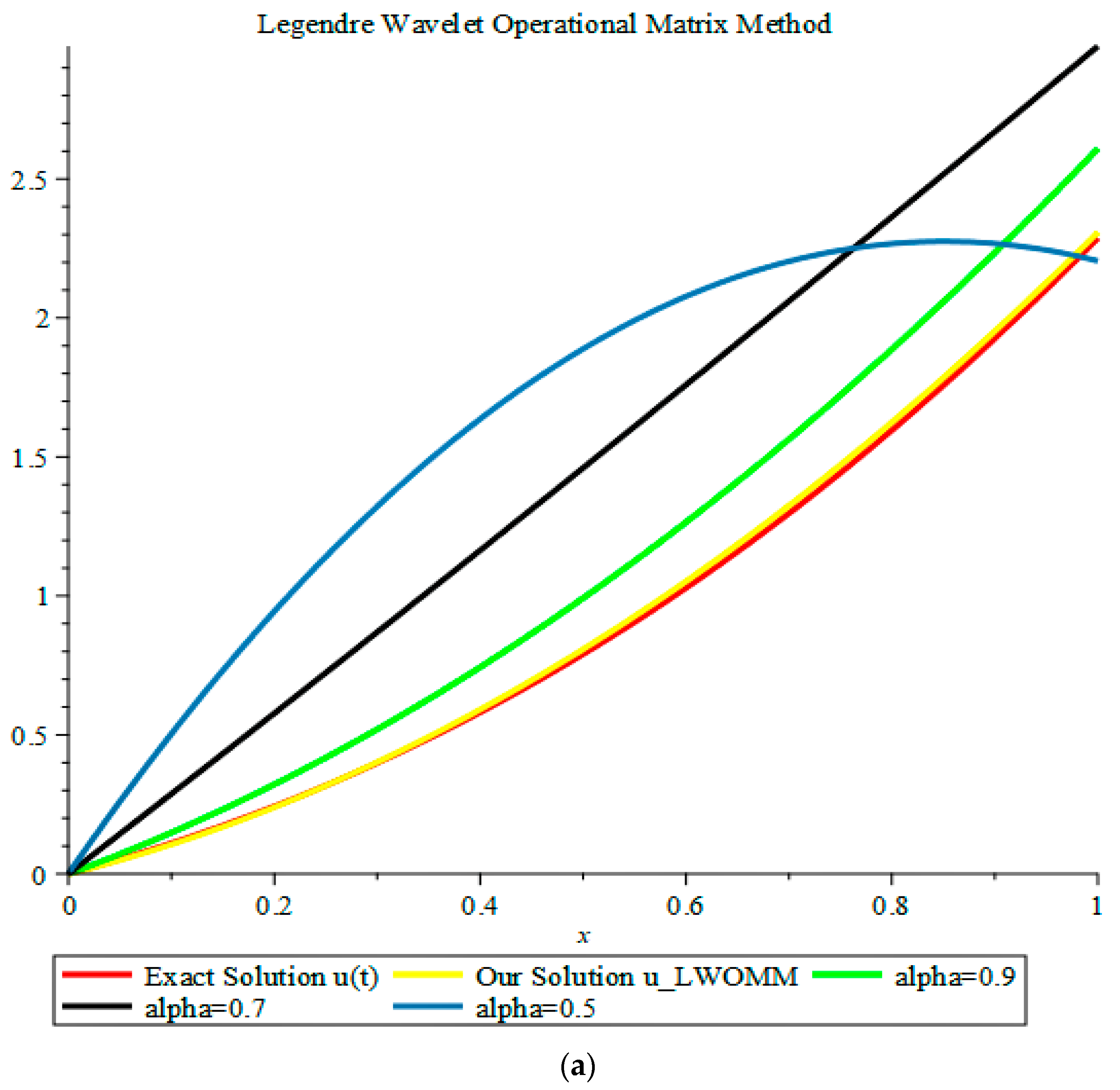
This example was examined for , , and . When the obtained results were matched against the exact solution when , as demonstrated in Figure 1, we can clearly observe that when approached 1, our results approached the exact solution. We also solved this problem by using Legendre polynomial operational matrix method (LPOMM), and we compared the results with the LWOMM. The numerical computations for u(t) and v(t) when are revealed in Table 1 and Table 2.
Example 2.
The exact solution of this system is known to be
Using the parameters and , we applied both the proposed method and the LPOMM to solve this problem and show that our approach is more efficient and useful. Our numerical results supported the idea that our solution approaches the exact solution more than the approximate solution LPOMM. Comparisons of the approximate and exact solutions are presented in Table 3 and Table 4.
Example 3.
We considered the following nonlinear system of fractional differential equations with the initial conditions [8]
The exact solution of this system when is known to be
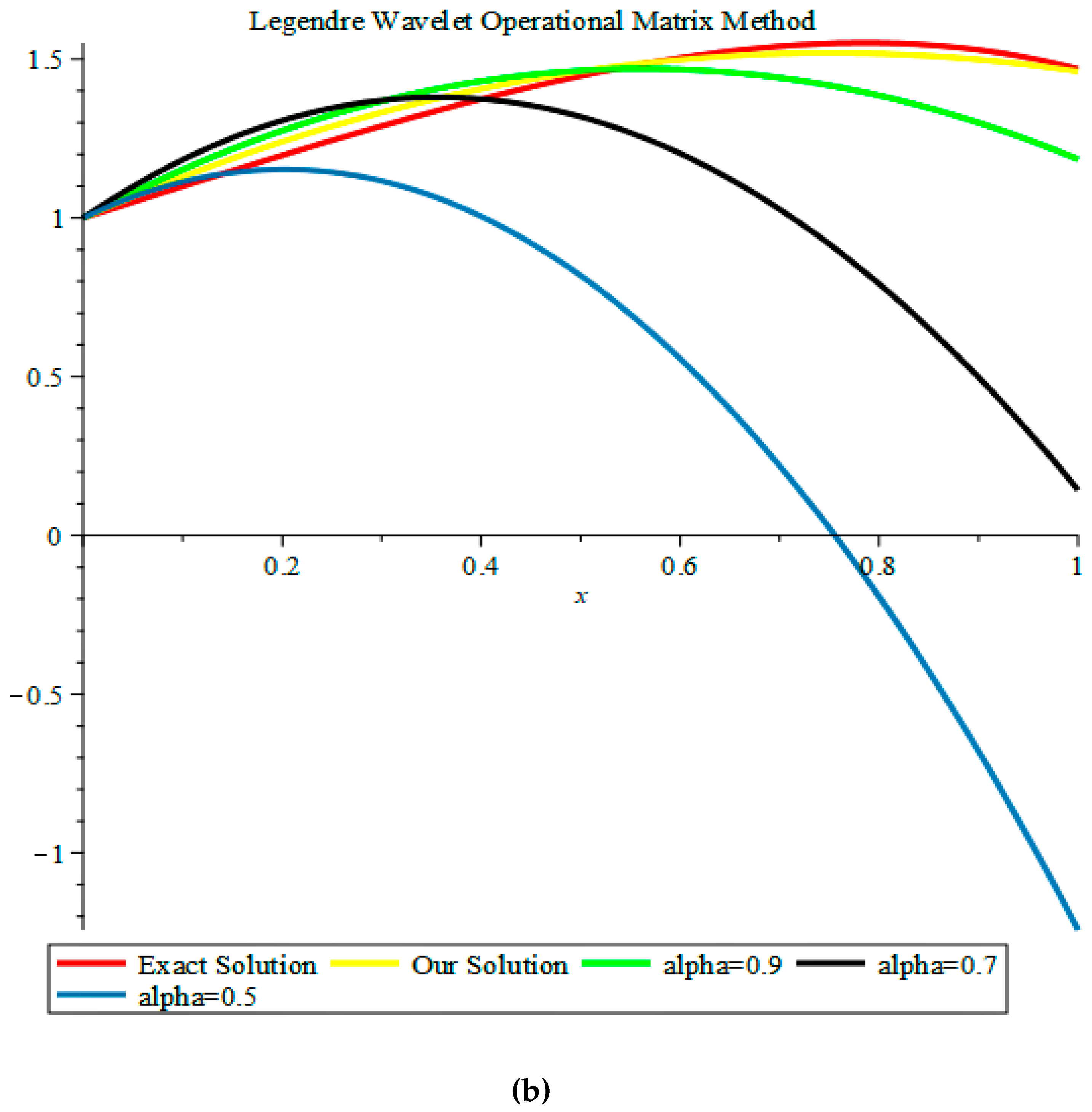
The parameters , and were utilized. A comparison of our results and the exact solution when is displayed in Figure 2. The figures support that when approximated 1, our results approximated the exact solution. We also solved this problem by using the LPOMM, and compared the results to the LWOMM. Finally, we present the numerical computations for u(t) and v(t) when in Table 5 and Table 6.
Example 4.
The exact solution of this system when is known to be
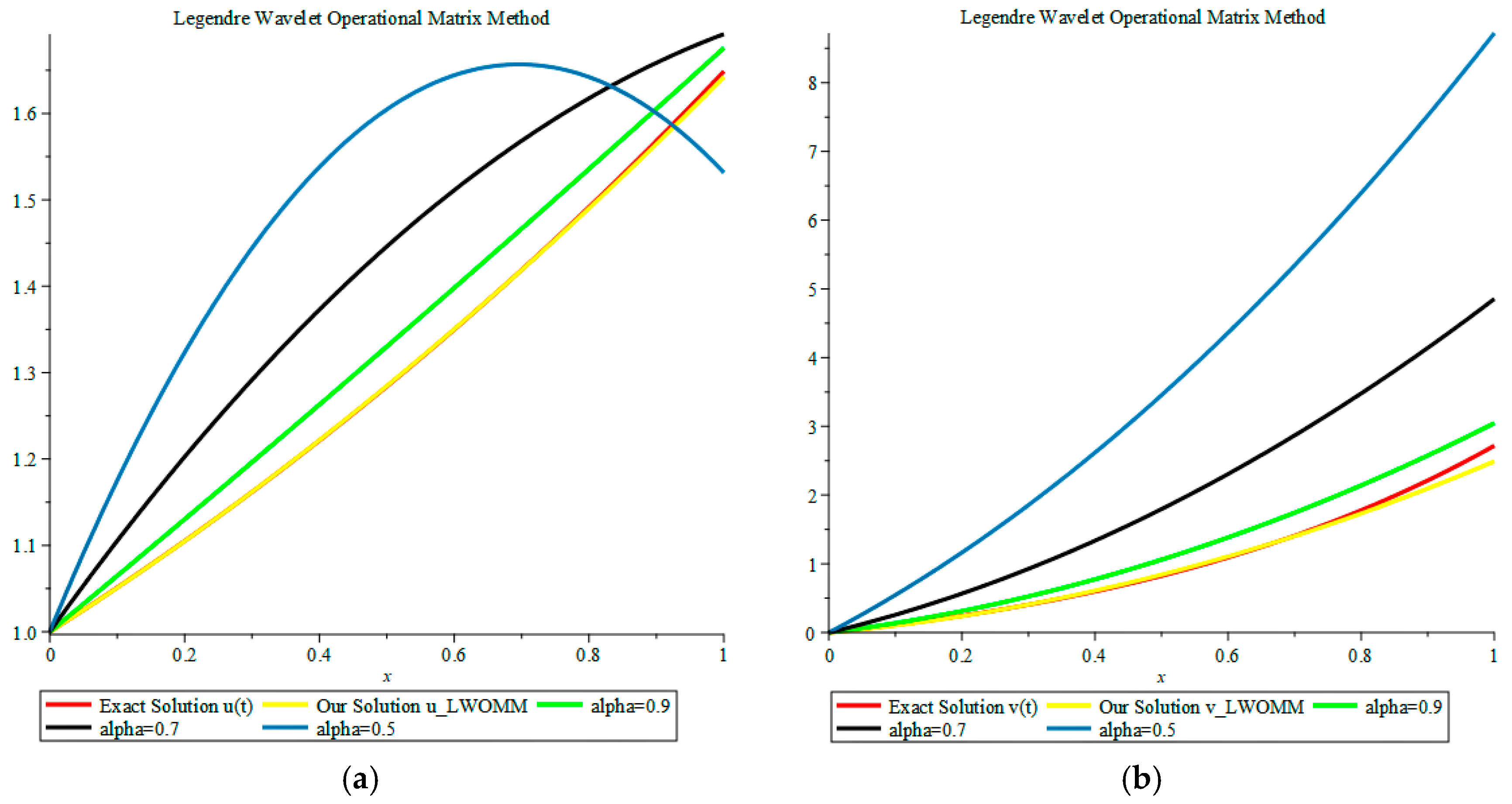
This example was analyzed for , , and . When the obtained results were matched against the exact solution when , as demonstrated in Figure 3, we can clearly observe that when approached 1, our results approached the exact solution. We also solved this problem by using the LPOMM, and compared the results with the LWOMM. The numerical computations for u(t) and v(t) when are also revealed in Table 7 and Table 8.
6. Conclusions
In this paper, a system of fractional_order differential equations was examined by drawing from a new operational matrix of the fractional derivative in some special conditions. We also systematized a very operational algorithm in order to attain the solution of the linear and nonlinear systems of fractional differential equations in Maple. All numerical results and graphical presentations generated by Maple affirmed that the Legendre wavelet operational matrix method is very effective and applicable. As the next step, the method introduced in this paper can be applied to fractional partial differential equations and the system of such equations, fractional integral equations and the system of such equations, and fractional integro-differential equations. These equations are at least as important as fractional differential equations and they are very significant in science, engineering, and technology.
Author Contributions
All authors contributed equally to the writing of this paper. All authors read and approved the final manuscript.
Funding
This research received no external funding.
Conflicts of Interest
The authors declare no conflict of interest.
References
- Song, L.; Wang, W. A new improved Adomian decomposition method and its application to fractional differential equations. Appl. Math. Model. 2013, 37, 1590–1598. [Google Scholar] [CrossRef]
- Balaji, S. Legendre wavelet operational matrix method for solution of fractional order Riccati differential equation. J. Eqypt. Math. Soc. 2015, 23, 263–270. [Google Scholar] [CrossRef]
- Rehman, M.; Khan, R.A. The Legendre wavelet method for solving fractional differential equations. Commun. Nonlinear Sci. Numer. Simul. 2011, 16, 4163–4173. [Google Scholar] [CrossRef]
- Mohammadi, F.; Hosseini, M.M.; Mohyud-Din, S.T. A new operational matrix for Legendre wavelets and its applications for solving fractional order boundary value problems. Int. J. Syst. Sci. 2011, 32, 7371–7378. [Google Scholar] [CrossRef]
- Şenol, M.; Dolapçı, İ.T. On the perturbation-iteration algorithm for fractional differential equations. J. King Saud Univ.-Sci. 2016, 28, 69–74. [Google Scholar] [CrossRef]
- Khader, M.M.; Danaf, T.S.; Hendy, A.S. A computational matrix method for solving systems of high order fractional differential equations. Appl. Math. Model. 2013, 37, 4035–4050. [Google Scholar] [CrossRef]
- Ertürk, V.S.; Momani, S. Solving systems of fractional differential equations using differential transform method. J. Comput. Appl. Math. 2008, 215, 142–151. [Google Scholar] [CrossRef]
- Gupta, S.; Kumar, D.; Singh, J. Numerical study for systems of fractional differential equations via Laplace transform. J. Egypt. Math. Soc. 2015, 23, 256–262. [Google Scholar] [CrossRef]
- Ghazanfari, B.; Ghazanfari, A.G. Solving system of fractional differential eqautions by fractional complex transform method. Asian J. Appl. Sci. 2012, 5, 438–444. [Google Scholar] [CrossRef]
- Kilbas, A.A.; Srivastava, H.M.; Trujillo, J.J. Theory and Applications of Fractional Differential Equations, 1st ed.; Elsevier Science: Amsterdam, The Netherlands, 2006; p. 540. [Google Scholar]
- Saadatmandi, A.; Dehghan, M. A new operational matrix for solving fractional-order differential equations. Comput. Math. Appl. 2010, 59, 1326–1336. [Google Scholar] [CrossRef]
- Alshbool, M.H.T.; Bataineh, A.S.; Hashim, I.; Işık, O.R. Solution of fractional-order differential equations based on the operational matrices of new fractional Bernstein functions. J. King Saud Univ.-Sci. 2017, 29, 1–18. [Google Scholar] [CrossRef]
- Isah, A.; Phang, C. New operational matrix of derivative for solving non-linear fractional differential equations via Genocchi polynomials. J. King Saud Univ.-Sci. 2017. [Google Scholar] [CrossRef]
- Doha, E.H.; Bhrawy, A.H.; Ezz-Eldien, S.S. A new Jacobi operational matrix: An application for solving fractional differential equations. Appl. Math. Model. 2012, 36, 4931–4943. [Google Scholar] [CrossRef]
- Mohammadi, F. Numerical solution of Bagley-Torvik equation using Chebyshev wavelet operational matrix of fractional derivative. Int. J. Adv. Appl. Math. Mech. 2014, 2, 83–91. [Google Scholar]
- Bota, C.; Caruntu, B. Approximate analytical solutions of the fractional-order brusselator system using the polynomial least squares method. Corp. Adv. Differ. Equ. 2015. [Google Scholar] [CrossRef]
- Chang, P.; Isah, A. Legendre wavelet operational matrix of fractional derivative through wavelet-polynomial transformation and its applications in solving fractional order brusselator system. J. Phys. Conf. Ser. 2016, 693, 012001. [Google Scholar] [CrossRef]
- Isah, A.; Phang, C. Genocchi wavelet-like operational matrix and its application for solving non-linear fractional differential equations. Open Phys. 2016, 14, 463–472. [Google Scholar] [CrossRef]
- Miller, K.S.; Ross, B. An Introduction to the Fractional Calculus and Fractional Differential Equations, 1st ed.; Wiley: Hoboken, NJ, USA, 1993; p. 384. [Google Scholar]
- Oldham, K.B.; Spanier, J. The Fractional Calculus, 1st ed.; Academic Press: New York, NY, USA, 1974; p. 234. [Google Scholar]
- Mohammadi, F.; Hosseini, M.M. A new Legendre wavelet operational matrix of derivative and its applications in solving the singular ordinary differential equations. J. Frankl. Inst. 2011, 348, 1787–1796. [Google Scholar] [CrossRef]
- Mohammadi, F.; Hosseini, M.M.; Mohyud-Din, S.T. Legendre wavelet Galerkin method for solving ordinary differential equations with non-analytic solution. Int. J. Syst. Sci. 2011, 42, 579–585. [Google Scholar] [CrossRef]
Figure 1.
Comparison of our solutions and the exact solution when in Example 1: (a) Our solution u(t); and (b) Our solution v(t).
Figure 1.
Comparison of our solutions and the exact solution when in Example 1: (a) Our solution u(t); and (b) Our solution v(t).


Figure 2.
Comparison of our solutions to the exact solution when for Example 3: (a) Our solution u(t); and (b) Our solution v(t).
Figure 2.
Comparison of our solutions to the exact solution when for Example 3: (a) Our solution u(t); and (b) Our solution v(t).

Figure 3.
Comparison of our solutions to the exact solution when for Example 4: (a) Our solution u(t); and (b) Our solution v(t).
Figure 3.
Comparison of our solutions to the exact solution when for Example 4: (a) Our solution u(t); and (b) Our solution v(t).

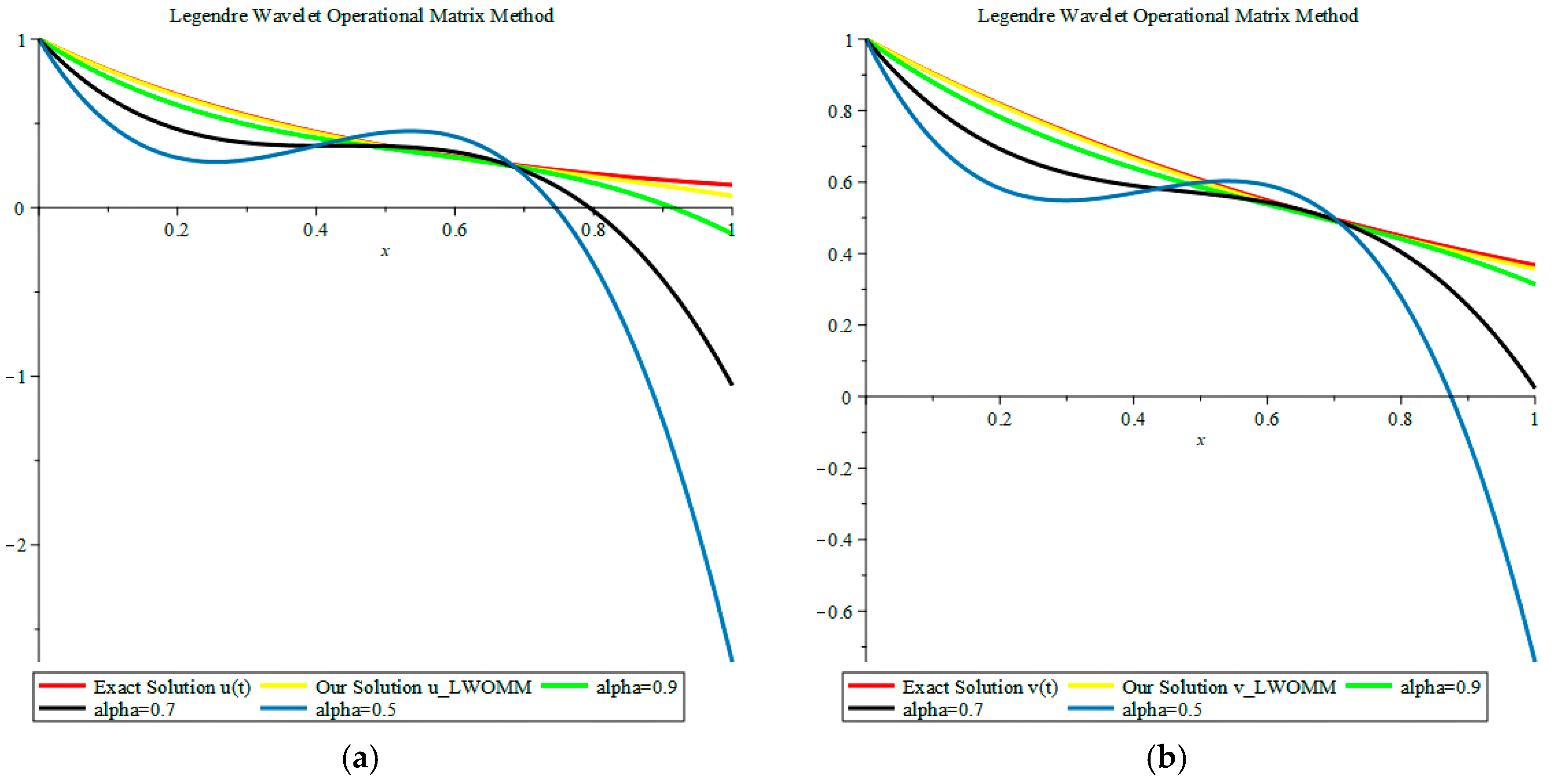
Figure 4.
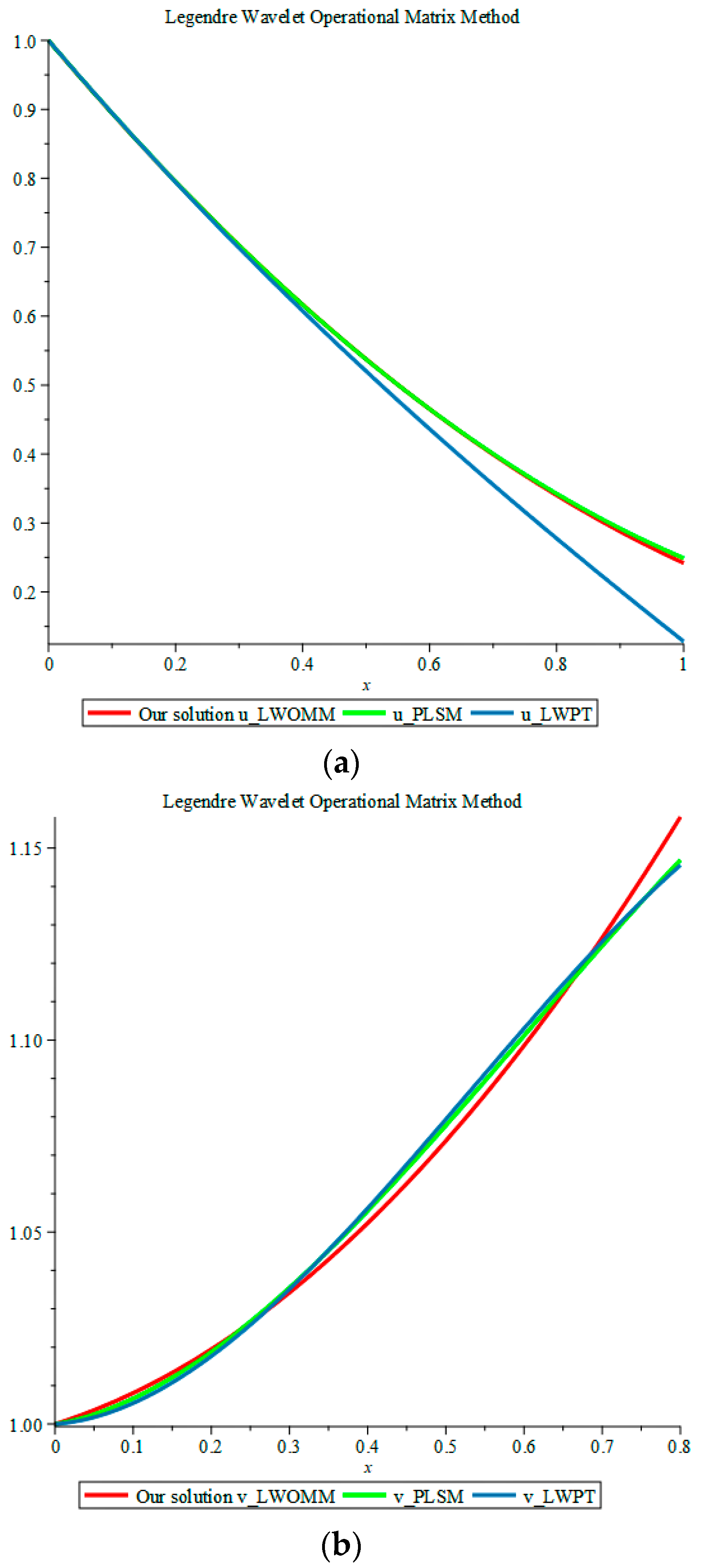
Comparison of our solutions to the approximate solution LWPT and the approximate solution PLSM when for Example 5: (a) Our solution u(t); and (b) Our solution v(t).
Figure 4.
Comparison of our solutions to the approximate solution LWPT and the approximate solution PLSM when for Example 5: (a) Our solution u(t); and (b) Our solution v(t).


Table 1.
Numerical solutions of u(t) when attained by the introduced method and the LPOMM for Example 1.
Table 1.
Numerical solutions of u(t) when attained by the introduced method and the LPOMM for Example 1.
| Absolute Error | |||
|---|---|---|---|
| 0.0 | 0.3 × | 0.0000000000 | 0.3 × |
| 0.1 | 0.1483784330 | 0.1483784325 | 0.12 × |
| 0.2 | 0.3217645283 | 0.3217645277 | 0.633 × |
| 0.3 | 0.5201582862 | 0.5201582855 | 0.65 × |
| 0.4 | 0.7435597067 | 0.7435597059 | 0.83 × |
| 0.5 | 0.9919687898 | 0.9919687890 | 0.8 × |
| 0.6 | 1.265385536 | 1.265385535 | 0.53 × |
| 0.7 | 1.563809944 | 1.563809943 | 0.95 × |
| 0.8 | 1.887242014 | 1.887242014 | 0.733 × |
| 0.9 | 2.235681748 | 2.235681748 | 0.62 × |
| 1.0 | 2.609129144 | 2.609129144 | 0.3 × |
Table 2.
Numerical solutions of v(t) when attained by the introduced method and the LPOMM for Example 1.
Table 2.
Numerical solutions of v(t) when attained by the introduced method and the LPOMM for Example 1.
| Absolute Error | |||
|---|---|---|---|
| 0.0 | 1.000000000 | 1.000000000 | 0.2 × |
| 0.1 | 1.152270899 | 1.152270900 | −0.5 × |
| 0.2 | 1.274801858 | 1.274801858 | 0.599 × |
| 0.3 | 1.367592877 | 1.367592878 | −0.67 × |
| 0.4 | 1.430643956 | 1.430643957 | −0.13 × |
| 0.5 | 1.463955094 | 1.463955094 | −0.1 × |
| 0.6 | 1.467526291 | 1.467526293 | −0.13 × |
| 0.7 | 1.441357549 | 1.441357551 | −0.171 × |
| 0.8 | 1.385448866 | 1.385448868 | −0.1461 × |
| 0.9 | 1.299800244 | 1.299800245 | −0.15 × |
| 1.0 | 1.184411680 | 1.184411682 | −0.18 × |
Table 3.
The numerical results attained by using the introduced method in comparison to the approximate solution LPOMM and the exact solution u(t) in Example 2.
Table 3.
The numerical results attained by using the introduced method in comparison to the approximate solution LPOMM and the exact solution u(t) in Example 2.
| Exact Solution | |||
|---|---|---|---|
| 0.0 | 0.000 | −0.12 × | 0.000000000000 |
| 0.1 | 0.001 | 0.01000000005 | 0.001000000000 |
| 0.2 | 0.008 | 0.02000000016 | 0.008000000000 |
| 0.3 | 0.027 | 0.03750000021 | 0.027000000000 |
| 0.4 | 0.064 | 0.07000000020 | 0.064000000000 |
| 0.5 | 0.125 | 0.12500000001 | 0.125000000000 |
| 0.6 | 0.216 | 0.21000000000 | 0.216000000000 |
| 0.7 | 0.343 | 0.33249999998 | 0.343000000000 |
| 0.8 | 0.512 | 0.49999999996 | 0.512000000000 |
| 0.9 | 0.729 | 0.71999999993 | 0.729000000000 |
| 1.0 | 1.000 | 0.99999999989 | 1.000000000000 |
Table 4.
The numerical results attained by using the introduced method in comparison with the approximate solution LPOMM and exact solution v(t) in Example 2.
Table 4.
The numerical results attained by using the introduced method in comparison with the approximate solution LPOMM and exact solution v(t) in Example 2.
| Exact Solution | |||
|---|---|---|---|
| 0.0 | 1.000 | 1.000000000 | 0.9999999998 |
| 0.1 | 1.002 | 1.034841367 | 1.165803114 |
| 0.2 | 1.016 | 1.057587628 | 1.283854751 |
| 0.3 | 1.054 | 1.086537668 | 1.374911456 |
| 0.4 | 1.128 | 1.139990370 | 1.459729770 |
| 0.5 | 1.250 | 1.236244618 | 1.559066242 |
| 0.6 | 1.432 | 1.393599296 | 1.693677414 |
| 0.7 | 1.686 | 1.630353290 | 1.884319831 |
| 0.8 | 2.024 | 1.964805482 | 2.151750038 |
| 0.9 | 2.458 | 2.415254758 | 2.516724579 |
| 1.0 | 3.000 | 3.000000000 | 3.000000000 |
Table 5.
Our solutions u(t) when attained by the presented method and the LPOMM for Example 3.
| Absolute Error | |||
|---|---|---|---|
| 0.0 | 1.000000000 | 1.000000000 | −0.37 × |
| 0.1 | 1.064816320 | 1.064816320 | −0.132 × |
| 0.2 | 1.130248588 | 1.130248589 | −0.1375 × |
| 0.3 | 1.196296807 | 1.196296807 | 0.44 × |
| 0.4 | 1.262960974 | 1.262960975 | −0.808 × |
| 0.5 | 1.330241090 | 1.330241091 | −0.532 × |
| 0.6 | 1.398137156 | 1.398137156 | −0.168 × |
| 0.7 | 1.466649171 | 1.466649171 | −0.756 × |
| 0.8 | 1.535777134 | 1.535777134 | −0.1375 × |
| 0.9 | 1.605521046 | 1.605521046 | 0.468 × |
| 1.0 | 1.675880908 | 1.675880908 | 0.163 × |
Table 6.
Our solutions v(t) when attained by the presented method and the LPOMM for Example 3.
| Absolute Error | |||
|---|---|---|---|
| 0.0 | −0.1 × | 0.0000000000 | −0.1 × |
| 0.1 | 0.1381762603 | 0.1381762609 | −0.7 × |
| 0.2 | 0.3133603361 | 0.3133603363 | −0.2 × |
| 0.3 | 0.5255522259 | 0.5255522263 | −0.37 × |
| 0.4 | 0.7747519304 | 0.7747519309 | −0.5 × |
| 0.5 | 1.060959450 | 1.060959450 | −0.5 × |
| 0.6 | 1.384174783 | 1.384174784 | −0.8 × |
| 0.7 | 1.744397932 | 1.744397932 | −0.47 × |
| 0.8 | 2.141628894 | 2.141628895 | −0.7 × |
| 0.9 | 2.575867672 | 2.575867672 | 0.3 × |
| 1.0 | 3.047114264 | 3.047114264 | −0.1 × |
Table 7.
Numerical solutions of u(t) when for Example 4.
| Absolute Error | |||
|---|---|---|---|
| 0.0 | 1.000000000 | 1.000000000 | −0.4 × |
| 0.1 | 0.8144351529 | 0.8144351528 | −0.21 × |
| 0.2 | 0.6639425233 | 0.6639425233 | −0.15 × |
| 0.3 | 0.5429947229 | 0.5429947230 | −0.34 × |
| 0.4 | 0.4460643636 | 0.4460643636 | −0.42 × |
| 0.5 | 0.3676240568 | 0.3676240568 | 0 |
| 0.6 | 0.3021464142 | 0.3021464147 | −0.68 × |
| 0.7 | 0.2441040487 | 0.2441040481 | −0.24 × |
| 0.8 | 0.1879695699 | 0.1879695690 | 0.53 × |
| 0.9 | 0.1282155920 | 0.1282155905 | 0.461 × |
| 1.0 | 0.0593147248 | 0.0593147222 | 0.144 × |
Table 8.
Numerical solutions of v(t) when for Example 4.
| Absolute Error | |||
|---|---|---|---|
| 0.0 | 1.000000000 | 0.9999999999 | 0.79 × |
| 0.1 | 0.9025601837 | 0.9025601837 | 0.1498 × |
| 0.2 | 0.8152646487 | 0.8152646488 | −0.119 × |
| 0.3 | 0.7371116577 | 0.7371116578 | −0.8 × |
| 0.4 | 0.6670994737 | 0.6670994739 | −0.11 × |
| 0.5 | 0.6042263597 | 0.6042263600 | −0.24 × |
| 0.6 | 0.5474905785 | 0.5474905788 | −0.19 × |
| 0.7 | 0.4958903932 | 0.4958903935 | −0.26 × |
| 0.8 | 0.4484240664 | 0.4484240670 | −0.443 × |
| 0.9 | 0.4040898614 | 0.4040898620 | −0.5898 × |
| 1.0 | 0.3618860408 | 0.3618860417 | −0.719 × |
Table 9.
Numerical solutions of u(t) when obtained by the introduced method, the LWPT, and the PLSM for Example 5.
Table 9.
Numerical solutions of u(t) when obtained by the introduced method, the LWPT, and the PLSM for Example 5.
| 0.0 | 1.000000000 | 1.0000000 | 1.0000000000 |
| 0.1 | 0.8942024826 | 0.8947372 | 0.8944807482 |
| 0.2 | 0.7950696916 | 0.7945136 | 0.7953304656 |
| 0.3 | 0.7026016268 | 0.6989464 | 0.7026953614 |
| 0.4 | 0.6167982883 | 0.6076528 | 0.6167216448 |
| 0.5 | 0.5376596761 | 0.5202500 | 0.5375555250 |
| 0.6 | 0.4651857902 | 0.4363552 | 0.4653432112 |
| 0.7 | 0.3993766306 | 0.3555856 | 0.4002309126 |
| 0.8 | 0.3402321973 | 0.2775584 | 0.3423648384 |
| 0.9 | 0.2877524902 | 0.2018908 | 0.2918911978 |
| 1.0 | 0.2419375095 | 0.1282000 | 0.2489562000 |
Table 10.
Numerical solutions of v(t) when obtained by the introduced method, the LWPT, and the PLSM for Example 5.
Table 10.
Numerical solutions of v(t) when obtained by the introduced method, the LWPT, and the PLSM for Example 5.
| 0.0 | 1.000000000 | 1.0000000 | 1.000000000 |
| 0.1 | 1.008069307 | 1.0054326 | 1.006641096 |
| 0.2 | 1.019479961 | 1.0176608 | 1.018844188 |
| 0.3 | 1.034231959 | 1.0351102 | 1.035502792 |
| 0.4 | 1.052325304 | 1.0562064 | 1.055510424 |
| 0.5 | 1.073759995 | 1.0793750 | 1.077760600 |
| 0.6 | 1.098536032 | 1.1030416 | 1.101146836 |
| 0.7 | 1.126653415 | 1.1256318 | 1.124562648 |
| 0.8 | 1.158112143 | 1.1455712 | 1.146901552 |
| 0.9 | 1.192912217 | 1.1612854 | 1.167057064 |
| 1.0 | 1.231053638 | 1.1712000 | 1.183922700 |
© 2018 by the authors. Licensee MDPI, Basel, Switzerland. This article is an open access article distributed under the terms and conditions of the Creative Commons Attribution (CC BY) license (http://creativecommons.org/licenses/by/4.0/).
Share and Cite
MDPI and ACS Style
Secer, A.; Altun, S. A New Operational Matrix of Fractional Derivatives to Solve Systems of Fractional Differential Equations via Legendre Wavelets. Mathematics 2018, 6, 238. https://0-doi-org.brum.beds.ac.uk/10.3390/math6110238
AMA Style
Secer A, Altun S. A New Operational Matrix of Fractional Derivatives to Solve Systems of Fractional Differential Equations via Legendre Wavelets. Mathematics. 2018; 6(11):238. https://0-doi-org.brum.beds.ac.uk/10.3390/math6110238
Chicago/Turabian StyleSecer, Aydin, and Selvi Altun. 2018. "A New Operational Matrix of Fractional Derivatives to Solve Systems of Fractional Differential Equations via Legendre Wavelets" Mathematics 6, no. 11: 238. https://0-doi-org.brum.beds.ac.uk/10.3390/math6110238
Note that from the first issue of 2016, this journal uses article numbers instead of page numbers. See further details here.