Accurate and Efficient Explicit Approximations of the Colebrook Flow Friction Equation Based on the Wright ω-Function

Abstract

The Colebrook equation is a popular model for estimating friction loss coefficients in water and gas pipes. The model is implicit in the unknown flow friction factor, $f$. To date, the captured flow friction factor, $f$, can be extracted from the logarithmic form analytically only in the term of the Lambert $W$-function. The purpose of this study is to find an accurate and computationally efficient solution based on the shifted Lambert $W$-function also known as the Wright ω-function. The Wright ω-function is more suitable because it overcomes the problem with the overflow error by switching the fast growing term, $y=W\left(e^x\right)$, of the Lambert $W$-function to series expansions that further can be easily evaluated in computers without causing overflow run-time errors. Although the Colebrook equation transformed through the Lambert $W$-function is identical to the original expression in terms of accuracy, a further evaluation of the Lambert $W$-function can be only approximate. Very accurate explicit approximations of the Colebrook equation that contain only one or two logarithms are shown. The final result is an accurate explicit approximation of the Colebrook equation with a relative error of no more than 0.0096%. The presented approximations are in a form suitable for everyday engineering use, and are both accurate and computationally efficient.

1. Introduction

The Colebrook equation; Equation (1), is an empirical relation which, in its native form, relates implicitly the unknown Darcy’s flow friction factor, $f$, with the known Reynolds number, $R$, and the known relative roughness of inner pipe surface, ${\epsilon }^{*}$ [1,2]. Engineers use it at defined domains of the input parameters: 4000 < $R$ < 10⁸ and for 0 < ${\epsilon }^{*}$ < 0.05. The Colebrook equation is transcendental (cannot be expressed in terms of elementary functions); the implicitly given function in respect to the unknown flow friction factor, $f$:

$$\frac{1}{\sqrt{f}}=-2·{\log }_{10}\left(\frac{2.51}{R}·\frac{1}{\sqrt{f}}+\frac{{\epsilon }^{*}}{3.71}\right)$$

(1)

The Colebrook equation; Equation (1) also has an exact explicit analytical form in the terms of the Lambert $W$-function; Equation (2) [3,4], which is also transcendental, but which can be evaluated using numerous thoroughly tested procedures with varying accuracy and complexity, developed for various applications in physics and engineering [5] (it is here also given in the terms of the Wright ω-function).

$$\begin{gathered} \begin{array}{c}\frac{1}{\sqrt{f}}=\frac{2}{\ln \left(10\right)}·\ln \left(\frac{R}{2.51}·\frac{\ln \left(10\right)}{2}\right)+W\left(e^x\right)-x \\ x=\ln \left(\frac{R}{2.51}·\frac{\ln \left(10\right)}{2}\right)+\frac{R·{\epsilon }^{*}}{2.51·3.71}·\frac{\ln \left(10\right)}{2}\end{array}\}\to \\ \begin{array}{c}\frac{1}{\sqrt{f}}=\frac{2}{\ln \left(10\right)}·\ln \left(\frac{R}{2.51}·\frac{\ln \left(10\right)}{2}\right)+\omega \left(x\right)-x \\ x=\ln \left(\frac{R}{2.51}·\frac{\ln \left(10\right)}{2}\right)+\frac{R·{\epsilon }^{*}}{2.51·3.71}·\frac{\ln \left(10\right)}{2}\end{array}\} \end{gathered}$$

(2)

The parameter, $x$, in Equation (2) depends on the input parameters; the Reynolds number, $R$, and the relative roughness of the inner pipe surface, ${\epsilon }^{*}$. Its domain is 7.51 < $x$< 618,187.84. The Lambert $W$-based Colebrook equation; Equation (2), contains the fast growing term, $W\left(e^x\right)$, which cannot be accurately stored in common computer registers due to the runtime overflow error for the particular combinations of the Reynolds number, $R$, and the relative roughness of the inner pipe surface, ${\epsilon }^{*}$, that can easily occur in everyday engineering practice [6,7]. The problem can be solved using the Wright ω-function, a cognate of the Lambert $W$-function, which uses a shifted, non fast-growing argument [4,8,9].

According to the very recently published study of Belkić [10], the Lambert $W$-function plays a very important role across interdisciplinary research. The reference gives an updated detailed list of applications, which include mathematics, physics, astrophysics, chemistry, biology, medicine, population genetics, ecology, sociology, education, energetics, and technology. Finally, the presented analytical solutions are numerically illustrated in the genome multiplicity corrections for survival of synchronous cell populations after irradiation [11].

This paper is oriented to the application of the Lambert $W$-function and the Wright ω-function in hydraulics (fluid dynamics). We present a few approximate solutions of the transformed Lambert $W$-based Colebrook equation in a form more suitable for the computing codes used in various engineering software. All mentioned and developed approximations are summarized in the Appendix A. The best version of the presented explicit approximation gives the value of the flow friction factor, f, for which the Colebrook equation is in balance with the relative error of no more than 0.0096%. Such accuracy achieved without using a large number of computationally expensive logarithmic functions (or non-integer powers) is highly computationally efficient. As reported by Clamond [12], Winning and Coole [13], Biberg [4], Vatankhah [14], etc., functions, such as logarithms and non-integer powers, require special algorithms with the execution of many more floating-point operations compared with basic arithmetic operations (+, −, ×, /) that are executed directly in the central processor unit (CPU) of computers.

In our previous contributions, we accelerated and simplified an iterative solution of the Colebrook equation. In [15], the Padé approximation is used as a cheap alternative to the logarithm in the second and the successful iterations of the fixed-point method. In [16], low cost starting points for iterative methods found by genetic approximations of the Colebrook equation are introduced and tested, while Praks and Brkić [17] discusses the optimal multi-point iterative methods for the Colebrook equation. Finally, advanced iterative procedures for the Colebrook equation are studied in [18].

Rather than improving iterative solutions, in this paper, we provide simple, but powerful approximations of the exact solution of the Colebrook model, which is given by the Wright ω-function. We introduce cheap yet still accurate approximations of the Wright ω-function for the Colebrook model using a symbolic regression technique [16,19,20] and Padé approximation [15,21]. Apparently, this is the first highly accurate explicit approximation of the Colebrook equation that contains only two computationally expensive functions (two logarithms, or as an alternative, two functions with non-integer powers), or even less if a combination of Padé approximations [15,21,22], and symbolic regression is used for a further reduction of the computational burden (where one of the logarithms is approximated by simple rational functions with a moderate increase of the maximal relative error).

2. Proposed Explicit Approximations and Comparative Analysis

The Colebrook equation in the terms of the Lambert $W$-function was apparently first proposed in 1998 by Keady [3]. However, as confirmed by Sonnad and Goudar [6] and Brkić [7], the term, $W\left(e^x\right)$, grows so fast that it cannot be evaluated easily, even in the registers of modern computers, due to the overflow runtime error for a particular number of combinations of the input parameters; the Reynolds number, $R$, and the relative roughness of the inner pipe surface, ${\epsilon }^{*}$; where parameter $x$ of Equation (2) depends directly on them. The procedure presented here replaces this fast growing term with the much more numerically stable Wright ω-function [23].

As noted by Lawrence et al. [15], the Wright ω-function was studied implicitly, without being named, by Wright [24], and named and defined by Corless and Jeffrey [25].

Further, the Colebrook equation, transformed explicitly in terms of the Lambert $W$-function, can be found, among others, in Keady [3], Goudar and Sonnad [26,27], Brkić [28,29,30,31,32], More [33], Sonnad and Goudar [34,35], Clamond [12], Rollmann and Spindler [9], Mikata and Walczak [36], and Biberg [4] and Vatankhah [14].

2.1. Transformation and Formulation

The shifted Wright ω-function transforms the argument, $e^x$, to $x$ in the series, $W\left(e^x\right)=\omega \left(x\right)\approx \ln \left(e^x\right)-\ln \left(\ln \left(e^x\right)\right)+\frac{\ln \left(\ln \left(e^x\right)\right)}{\ln \left(e^x\right)}$; where $x=\ln \left(e^x\right)$. Thus, the undesirably fast growing term, $W\left(e^x\right)$, in Eqation (2) is approximated accurately through $y\approx x-\ln \left(x\right)+\frac{\ln \left(x\right)}{x}$. The transformation is based on unsigned Stirling numbers of the first kind as reported by Rollmann and Spindler [9].

Table 1. Values of $W\left(e^x\right)$ compared with its approximate replacement, $y\approx x-\ln x+\frac{\ln x}{x}$.

$\mathit{W}\mathbf{\left(}{\mathit{e}}^{\mathit{x}}\mathbf{\right)}$	R = 4000	R = 104	R = 105	R = 106	R = 107	R = 108
${\epsilon }^{*}=$10−6	5.763586714	6.552354737	8.594740889	10.78188015	13.94025768	26.71930109
${\epsilon }^{*}=$10−5	5.767379666	6.562009418	8.694474328	11.80401384	24.50329461	125.7849498
${\epsilon }^{*}=$10−3	5.805329409	6.658658836	9.697953496	22.29514802	124.0554132	#VALUE!
${\epsilon }^{*}=$10−2	6.186774452	7.63459358	20.09639172	122.325789	#VALUE!	#VALUE!
${\epsilon }^{*}=$0.05	10.14320931	17.90904123	120.5960672	#VALUE!	#VALUE!	#VALUE!
$\mathit{y}$	R = 4000	R = 104	R = 105	R = 106	R = 107	R = 108
${\epsilon }^{*}=$10−6	5.766606874	6.552971455	8.592338256	10.7784212	13.93654591	26.71669441
${\epsilon }^{*}=$10−5	5.770385511	6.562602762	8.691991603	11.80037821	24.50049484	136.3596559
${\epsilon }^{*}=$10−3	5.808193728	6.659024862	9.694862641	22.29214094	134.073966	1246.853296
${\epsilon }^{*}=$10−2	6.188374207	7.633218988	20.093168	131.7885643	1244.552558	12,371.62215
${\epsilon }^{*}=$0.05	10.13993873	17.90560354	129.5034606	1242.251823	12,369.31975	123,639.9564

Note: #VALUE!—Overflow error.

shows the values of $W\left(e^x\right)$ compared with its approximate replacement in the domain of the applicability of the Colebrook equation. Without the proposed transformation and simplification, the runtime overflow error occurs during the evaluation of the friction factor, $f$, in computers for particular pairs or the Reynolds number, $R$, and the relative roughness of the inner pipe surface, ${\epsilon }^{*}$; where the parameter, x, of Equation (2) depends directly on them (#VALUE! is an overflow error in Table 1). The values in Table 1 were calculated in MS Excel.

The simplifications; $W\left(e^x\right)-x\approx \ln \left(x\right)·\left(\frac{1}{x}-1\right)$; $\frac{2}{\ln 10}\approx 0.8686$; $\frac{2·2.51}{\ln 10}\approx 2.18$; and $2.18·3.71\approx 8.0878$, and $\ln \left(\frac{2·2.51}{\ln 10}\right)\approx 0.7794$; transform the Lambert $W$-based expression of the Colebrook equation in a very accurate explicit approximate form that can be used efficiently in everyday engineering practice; Equation (3):

$$\begin{array}{c}\frac{1}{\sqrt{f}}\approx 0.8686·\left[B-C+\frac{C}{B+A}\right]\\ A\approx \frac{R·{\epsilon }^{*}}{8.0878}\\ \begin{array}{c}B\approx \ln \left(\frac{R·\ln 10}{2·2.51}\right)\approx \ln \left(R\right)-0.7794\\ C=\ln \left(B+A\right)\end{array}\end{array}\}$$

(3)

Instead of logarithmic functions in the proposed explicit approximation; Equation (3), a new form for $B$ and $C=\ln \left(B+A\right)$ can be introduced, where $a$ can be any sufficiently large constant, where the larger value of $a$ gives a more accurate approximation of the logarithmic function, Equation (4):

$$\begin{array}{c}B\approx a·R^{a^{-1}}-a-0.7794\\ C=\ln \left(B+A\right)\approx a·{\left(B+A\right)}^{a^{-1}}-a\end{array}\}$$

(4)

Very accurate results were obtained for $a>{10}^5$. Choosing this value, power $a^{-1}=\frac{1}{a}$ is a fraction with an integer numerator and denominator, where the appropriate form depends on the programming language, and the option with fever floating point operations should be chosen [37].

Forms, such as $R^{0.00001}$, require an evaluation of two transcendental functions, because compilers in most programming languages interpret it through $e^{0.00001·\ln \left(R\right)}$ [12].

For more accurate results, $W\left(e^x\right)-x\approx \frac{1.038·\ln \left(x\right)}{x+0.332}-\ln \left(x\right)$ or $W\left(e^x\right)-x\approx \frac{1.0119·\ln \left(x\right)}{x}-\ln \left(x\right)+\frac{\ln \left(x\right)-2.3849}{x^2}$ can be used. These new approximations were found using the symbolic regression software, Eureqa [16,19,20], and they are 2.5 and 16.7 times more accurate, respectively, as compared with expression $y$ from Table 1. The related approximations are given with Equations (5) and (6), respectively.

$$\frac{1}{\sqrt{f}}\approx 0.8686·\left[B-C+\frac{1.038·C}{0.332+B+A}\right]$$

(5)

$$\frac{1}{\sqrt{f}}\approx 0.8686·\left[B-C+\frac{1.0119·C}{B+A}+\frac{C-2.3849}{{\left(B+A\right)}^2}\right]$$

(6)

In Equations (5) and (6), parameters $A$, $B$, and $C$ are the same as in Equation (3).

2.2. Accuracy

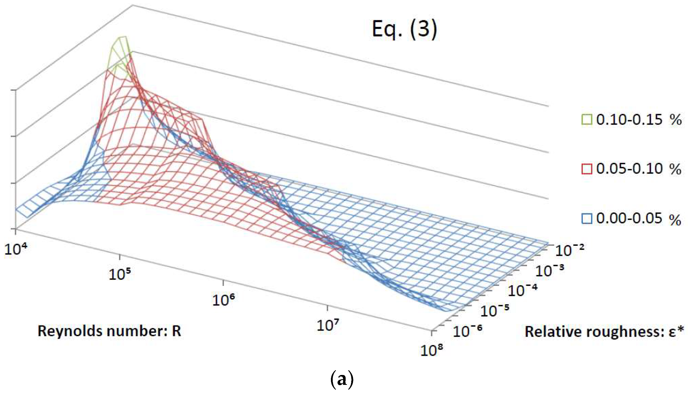
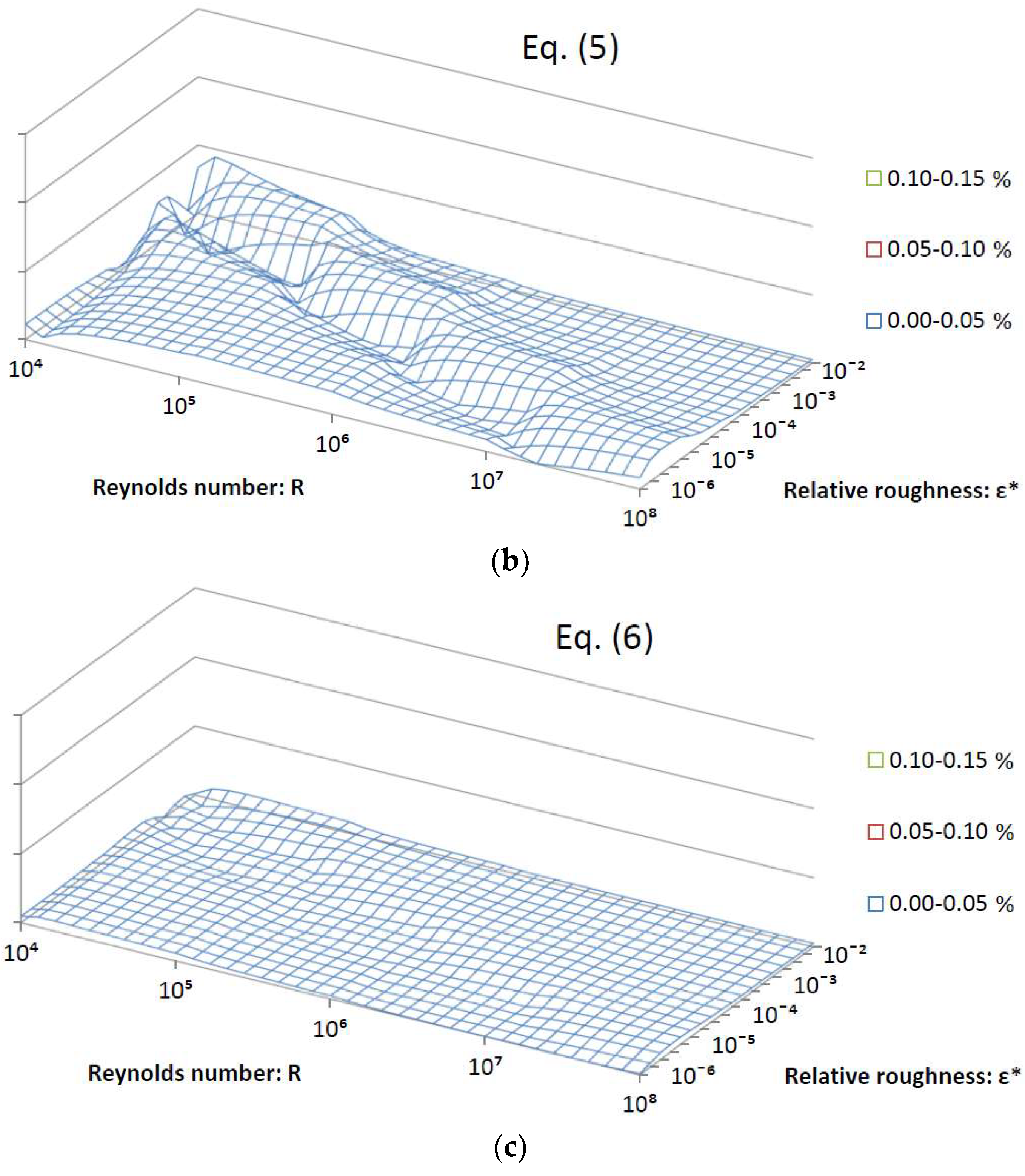
With the friction factor, f, computed using the approximate equations, Equation (3), the Colebrook equation is in balance with a relative error of no more than 0.13%, while using Equation (5) of no more than 0.045%, and finally, using Equation (6) of no more than 0.0096%, respectively. The related distribution of errors is shown in Figure 1. The presented approximations require evaluation of only two computationally expensive functions (two logarithms; Equations (3), (5), and (6), or alternatively two non-integer powers; Equation (4)), and therefore they are not only accurate, but also efficient for calculation.

The demonstrated approximation of Equation (3) based on the Wright ω-function with a relative error of up to 0.13% is about 10 times more accurate compared to the approximation from Brkić [30], while Equation (5) is more than 25 times more accurate than [30], and, finally, Equation (6) is more than 100 times more accurate than [30]. The approximations from Brkić [30,31] are based on the Lambert $W$-function.

The most accurate approximations available to date are by Vatankhah [14], Offor and Alabi [38], Buzzelli [39], Vatankhah and Kouchakzadeh [40], Romeo et al. [41], Zigrang and Sylvester [42], and Serghides [43]. All approximations mentioned [14,38,39,40,41,42,43,44,45,46,47] or developed in this paper are listed in the Appendix A, and their evaluated maximal relative error is shown in

Table 2. Number of computationally expensive functions in the available approximations of the Colebrook equations that introduce a relative error of no more than 1%.

1 Approximation	Maximal Relative Error %	Function
		Logarithms	Non-Integer Powers	2 TOTAL
Vatankhah [14]	0.0028%	1	2	3(5)
Here developed; Equation (6)	0.0096%	2	0	2
Here developed; Equation (5)	0.045%,	2	0	2
Offor and Alabi [38]	0.0602%	2	1	3(4)
Here developed; Equation (3)	0.13%	2	0	2
Here developed; Equation (4)	0.13%	0	2	2(4)
3 Buzzelli [39]	0.14%	2	0	2
Zigrang and Sylvester [42]	0.14%	3	0	3
Serghides [43]	0.14%	3	0	3
Romeo et al. [41]	0.14%	3	2	5(7)
Vatankhah and Kouchakzadeh [40]	0.15%	2	1	3(4)
Barr [44]	0.27%	2	2	4(6)
Serghides-simple [43]	0.35%	2	0	2
Chen [45]	0.36%	2	2	4(6)
Here developed; Equation (11)	Up to 0.4%	1	0	1
Fang et al. [46]	0.62%	1	3	4(7)
Papaevangelou et al. [47]	0.82%	2	1	3(4)

Notes: ¹ All approximations are listed in the Appendix A of this paper, ² in brackets: according to Clamond [12], non-integer powers require the evaluation of two computationally expensive functions–logarithm and exponential function, ³ in addition also contains one square root function.

.

Elaboration on the accuracy of explicit approximations to the Colebrook equation can be found, among others, in Zigrang and Sylvester [48], Gregory and Fogarasi [49], Brkić [50,51], Winning and Coole [13,52], Brkić and Ćojbašić [11], and Pimenta et al. [53].

2.3. Complexity and Computational Burden

In a computer environment, a logarithmic function and non-integer powers require more floating-point operations to be executed in the central processor unit (CPU) compared to simple arithmetic operations, such as adding, subtracting, multiplication, and division [12,13,14,54,55]. With a relative error of up to 0.0096%, the herein proposed explicit approximation of the Colebrook equation; Equation (6), that contains only two computationally expensive functions, is not only accurate, but also sufficiently efficient. Winning and Coole [13] reported relative effort for computation as: Addition-1, Subtraction-1.18, Division-1.35, Multiplication-1.55, Squared-2.18, Square root-2.29, Cubed-2.38, Natural logarithm-2.69, Cubed root-2.71, Fractional exponential-3.32, and Logarithm to base 10–3.37. One exception is Biberg [4], who grouped division with more expensive functions.

For comparison, Table 2 provides the number of logarithmic functions and non-integer terms used in available approximations. Table 2 shows only highly accurate approximations with a relative error of no more than 1%, according to criteria set by Brkić [50]. All approximations from Table 2 are given in the Appendix A of this article.

In addition to that presented here, the approximation by Brkić [28,30,32] is also based on the Lambert W-function, but as it uses four logarithmic functions, it is much more computationally expensive, and is significantly less accurate with a relative error of about 2.2%.

In the next Section, the term, $B\approx \ln \left(\frac{R·\ln 10}{2·2.51}\right)\approx \ln \left(R\right)-0.7794$, from Equation (3) is approximated very accurately through rational polynomial expression, so complexity and computational expense additionally decrease, as the logarithm is accurately approximated by a simple rational function. Numerical experiments show that for the here mentioned approximation $\ln \left(\frac{2·2.51}{\ln \left(10\right)}\right)\approx 0.7794$ is enough. For this reason we use this value in the Matlab codes shown in Section 3.

2.4. Simplifications

A simple rational approximation of the logarithm term, $B$, of the novel Colebrook approximation formulas; Equations (3), (5), and (6), is shown in this section. The logarithm represents the most computationally expensive operation of the Colebrook formula, see Equation (3). To reduce computation costs, the idea is to approximate the term, $B$, of Equation (3), which contains the logarithmic function, by a simple rational function. A combination of Padé approximation [15,21] and an artificial intelligence symbolic regression procedure [16,19,20] is used for this. Although the logarithm is a transcendental function, the found rational approximation remains simple and accurate with a maximal relative error limited to 0.2%. Although this rational approximation of the logarithm may seem unsightly to human eyes, it is very fast with computers, as it requires only a limited number of basic arithmetic operations to be executed in the central processor unit (CPU).

For the purpose of this simplification, the observed form, $B$, from Equation (3) can be transformed as; Equation (7):

$$\begin{array}{c}B\approx \ln \left(R\right)-\ln \left(2.18\right)=\ln \left(\mathrm{315,012.6}·r\right)-0.77932=\ln \left(r\right)+\ln \left(\mathrm{315,012.6}\right)-\\ 0.77932=\ln \left(r\right)+11.881\end{array}$$

(7)

In Equation (7), for the term, $r=\frac{R}{\mathrm{315,012.6}}$, the constant, 315,012.6, is carefully selected to minimize the error of the /2,3/ order Padé approximation of $\ln (r)$ at the expansion point, $r_0=1$. The proposed Padé approximant of the /2,3/ order of $\ln (r)$ at point 1 is; Equation (8):

$$\ln \left(r\right)\approx s\left(r\right)=\frac{r·\left(r·\left(11·r+27\right)-27\right)-11}{r·\left(r·\left(3·r+27\right)+27\right)+3}$$

(8)

The value, 315,012.6, is a weighted average of the Reynolds number, $R$, for the turbulent zone valid for the Colebrook equation; $R_{min}=4000$ and $R_{max}={10}^8$, using the value 0.0063 that was set by numerical experiments to minimize the absolute value of the maximum relative error of the Padé approximant of $\ln (r)$ in the interval, $\left[R_{min}, R_{max}\right]$, as $0.0063·\frac{R_{min}+R_{max}}{2}=315,012.6$. The Padé approximant approximates a certain function very accurately only in a relatively small domain of input parameters. It has been observed that the Padé approximant of $\ln \left(r\right)$ at the expansion point, $r_0=1$, defined by a rational function, $\mathrm{s}(r)$, approximates $\ln \left(r\right)$ with a maximal relative error of between −11.8% and 11.8% for all values of the Reynolds number, $R$, in the interval, $\left[R_{min}, R_{max}\right]$. The Padé approximant, $\mathrm{s}(r)$, has a negligible error for $r~1$, whereas top errors correspond to border points, $R_{min}$ and $R_{max}$. For example, for $R_{min}=4000$, the Padé approximant of $\ln \left(r\right)$ is $s\left(\frac{4000}{315,012.6}\right)=s\left(0.012697905\right)=-3.38744549$ where $R=315,012.6·r$. Therefore, the value of $\ln \left(4000\right)$ is approximated by $\ln \left(\mathrm{315,012.6}\right)+\left(-3.387445469\right)=9.272922448$. The corresponding relative error for $\ln \left(4000\right)$, is −11.8%.

Because of $B=\ln \left(\frac{R}{\frac{2·2.51}{\ln \left(10\right)}}\right)=\ln \left(R\right)-\ln \left(\frac{2·2.51}{\ln \left(10\right)}\right)$ and $\ln \left(\mathrm{315,012.6}\right)-\ln \left(\frac{2·2.51}{\ln \left(10\right)}\right)~11.881$, the value of $B$ can be approximated as Equation (9):

$$B\approx \ln \left(r\right)+11.881\approx s\left(r\right)+11.881$$

(9)

Further, a symbolic regression technique based on the computer software, Eureqa [19,20], is used for a more precise approximation of $\ln \left(r\right)$. The aim is to construct a more accurate rational approximation of $\ln (r)$ in comparison with Equation (9) using two known variables: The ratio, $r=\frac{R}{\mathrm{315,012.6}}$, and its Padé approximation, $\mathrm{s}\left(r\right)$. To reduce the burden for the central processor unit (CPU), the symbolic regression model should have a computationally cheap evaluation. For this reason, only rational functions are assumed for the symbolic regression model. To achieve that, 200 carefully selected quasi-random points of $r$ using the LPTAU51 algorithm were used [56,57]. For these generated numbers, the Padé approximation $\mathrm{s}\left(r\right)$ was calculated using Equation (8). Also, $\ln \left(r\right)$ was calculated to train the model in Eureqa for the purpose of finding a rational approximation of $\ln \left(r\right)$ by using $r$ and $\mathrm{s}(r)$ pairs. The developed models were successfully tested using 2048 quasi-random points. As a result, value $B$ was approximated by simple rational functions, Equation (10), with a negligible maximal relative error of 0.0765%:

$$B\approx 0.98236·s+\frac{s^7}{9200.67}+\frac{r}{150.2325}-\frac{r^2}{138187.1651}-\frac{1}{161.124·r}+11.881$$

(10)

Here, the symbol, $s$, denotes the Padé approximant, $s\left(r\right)$, given by Equation (8) and $r=\frac{R}{\mathrm{315,012.6}}$ is its argument.

When the Horner nested representation and the Variable Precision Arithmetic (VPA) at 4 decimal digit accuracy is assumed, the approximation of $B$ can be simplified by Equation (11):

$$B \approx s·\left(0.0001086·s^6 + 0.9824 \right)- \frac{0.006206 }{r} -r·\left(0.000007237·r - 0.006656\right) + 11.881,$$

(11)

In this case, the maximal relative error remains negligible, 0.0793% compared with $B$ calculated using Equation (3).

The combined approach with the Padé approximant and the symbolic regression introduced in this section is based on human observation and introducing the ratio, $r=\frac{R}{\mathrm{315,012.6}}$, with the subsequent symbolic regression of $r$ and $\mathrm{s}(r)$ pairs by Eureqa. The maximal relative error of $B$ introduced by Equation (11) was small (0.0793%), and in total if it is used instead of $B\approx \ln \left(\frac{R}{2.18}\right)$ from Equation (3), the total maximal error of the explicit approximation of the Colebrook equation can go up to 0.4%. As can be seen from Table 2, with the only one-log call for $\ln \left(B+A\right)$ from Equation (3), this extremely accurate explicit approximation of the Colebrook equation approximation is the cheapest for computation presented to date.

The combined approach presented herein, with Padé approximation and symbolic regression, can be also used for faster yet still accurate probabilistic modelling of gas networks, which requires a large number of model evaluations [58,59,60,61].

3. Software Description

The presented approximations are thoroughly tested and registered at IT4Innovations, VŠB–Technical University of Ostrava, Czech Republic. The codes are given in Matlab, but they can be easily transposed in any programming language. The symbol I.R denotes the vector of the Reynolds number $R$, whereas I.K denotes the vector of the relative roughness of the inner pipe surface ${\epsilon }^{*}$. The final result of the codes is the vector of the Darcy friction factor f.

The Matlab code for Equation (2), which presents the exact solution of the Colebrook equation using the Wrightomega function y = wrightOmega(x)-x is:

c.C = 2 * 2.51/log(10); c.logC = log(c.C); c.C371 = c.C * 3.71; c.Cd251 = c.C/2.51;

B = log(I.R) − c.logC;

A = I.R.* I.K./c.C371;

x = A + B;

y = wrightOmega(x) − x;

f = 1./(c.Cd251. * (B + y)).^2;

If needed, wrightOmega(x) can be replaced by: lambertw(exp(x)).

The Matlab code for Equation (3), which presents the approximation of the Colebrook equation using y = lnx./x − lnx, where the symbol lnx denotes the natural logarithm is:

c.Cd251 = 0.8686; c.logC = 0.7794; c.C371 = 8.0878;

B = log(I.R) − c.logC;

A = I.R. * I.K./c.C371;

x = A + B;

lnx = log(x);

y = (lnx./x − lnx);

f = 1./(c.Cd251. * (B + y)).^2;

The Matlab code for Equation (5), which presents the approximation of the Colebrook equation using y = (1.038 * lnx)./(x + 0.332) − lnx is the same like approximation using y = lnx./x − lnx, but the line y = (lnx./x-lnx) is replaced by: y = (1.038 * lnx)./(x + 0.332) − lnx

Matlab code for Equation (6) which presents the approximation of the Colebrook equation using y = (1.0119 * lnx)./x − lnx + (lnx−2.3849)./x.^2 is the same like approximation using y = lnx./x − lnx, but the line y= (lnx./x − lnx) is replaced by: y = (1.0119 * lnx)./x − lnx + (lnx − 2.3849)./x.^2

4. Conclusions

In this paper, we presented novel, precise, but still numerically inexpensive approximations of the Colebrook flow friction equation, which has been widely used in hydraulics since 1937 [1,2,3,4]. Our novel approach exploited the fact that the exact solution of the Colebrook equation can be expressed by the Lambert $W$-function [3,4] and combined numerical properties of the Wright ω-function [23,24,25], Padé approximation [15], and a symbolic regression technique [16,62].

The implicit Colebrook equation for flow friction is empirical, and hence has disputable accuracy. However, in many cases it is necessary to repeat calculations and to resolve the equation accurately to compare scientific results. An iterative solution [63] requires extensive computational effort, especially for flow evaluation of complex water or gas pipeline networks [64,65,66,67]. Although various available explicit approximations offer a good alternative, they are by the rule very accurate, but too complex, and vice versa [50]. Contrary to previous approximations of the Colebrook equation, the relation presented herein with a relative error limited to 0.0096% is amongst the most accurate available explicit approximations of the Colebrook equation. Moreover, the approach presented herein was also very computationally cheap, as it needs only one or two logarithms (or alternatively two non-integer powers). Measured against the criteria of accuracy and complexity, these approximations demonstrated desirable levels of performance. Consequently, the approximations can be recommended for implementation in software codes for engineering use.

The Colebrook equation is relevant only for turbulent flow, while for full-scale flow, different unified equations need to be used [68]. Consequently, the presented approximations are suitable for all cases where the Colebrook equation is used. Although the original experiment conducted by Colebrook and White used air [1,2], the Colebrook equation is today mostly used for modelling water flow [67]. However, in the case of natural gas flow modelling, the American Gas Association (AGA) and the American Bureau of Mines recommend replacing the coefficient of Equation (1) from 2.51 to 2.825 [69,70]. For future work, it would be interesting to integrate these novel flow friction models to stochastic gas network simulators [58,61].

Our approximations are valid for the whole domain of applicability of the Colebrook equation (on the other hand some of the approximations available from the scientific literature [71] are accurate only in certain narrow domain; e.g. for the highly turbulent flow or for the similar particular cases).

References

- Colebrook, C.F.; White, C.M. Experiments with fluid friction in roughened pipes. Proc. R. Soc. A Math. Phys. Eng. Sci. 1937, 161, 367–381. [Google Scholar] [CrossRef]
- Colebrook, C.F. Turbulent flow in pipes with particular reference to the transition region between the smooth and rough pipe laws. J. Inst. Civ. Eng. (Lond.) 1939, 11, 133–156. [Google Scholar] [CrossRef]
- Keady, G. Colebrook-White formula for pipe flows. J. Hydraul. Eng. 1998, 124, 96–97. [Google Scholar] [CrossRef]
- Biberg, D. Fast and accurate approximations for the Colebrook equation. J. Fluids Eng. 2017, 139, 031401. [Google Scholar] [CrossRef]
- Barry, D.A.; Parlange, J.Y.; Li, L.; Prommer, H.; Cunningham, C.J.; Stagnitti, F. Analytical approximations for real values of the Lambert W-function. Math. Comput. Simul. 2000, 53, 95–103. [Google Scholar] [CrossRef]
- Sonnad, J.R.; Goudar, C.T. Constraints for using Lambert W function-based explicit Colebrook–White equation. J. Hydraul. Eng. 2004, 130, 929–931. [Google Scholar] [CrossRef]
- Brkić, D. Comparison of the Lambert W-function based solutions to the Colebrook equation. Eng. Comput. 2012, 29, 617–630. [Google Scholar] [CrossRef]
- Corless, R.M.; Gonnet, G.H.; Hare, D.E.; Jeffrey, D.J.; Knuth, D.E. On the Lambert W function. Adv. Comput. Math. 1996, 5, 329–359. [Google Scholar] [CrossRef]
- Rollmann, P.; Spindler, K. Explicit representation of the implicit Colebrook–White equation. Case Stud. Therm. Eng. 2015, 5, 41–47. [Google Scholar] [CrossRef]
- Belkić, D. All the trinomial roots, their powers and logarithms from the Lambert series, Bell polynomials and Fox–Wright function: Illustration for genome multiplicity in survival of irradiated cells. J. Math. Chem. 2018. [Google Scholar] [CrossRef]
- Brkić, D.; Ćojbašić, Ž. Evolutionary optimization of Colebrook’s turbulent flow friction approximations. Fluids 2017, 2, 15. [Google Scholar] [CrossRef]
- Clamond, D. Efficient resolution of the Colebrook equation. Ind. Eng. Chem. Res. 2009, 48, 3665–3671. [Google Scholar] [CrossRef]
- Winning, H.K.; Coole, T. Improved method of determining friction factor in pipes. Int. J. Numer. Methods Heat Fluid Flow 2015, 25, 941–949. [Google Scholar] [CrossRef]
- Vatankhah, A.R. Approximate analytical solutions for the Colebrook equation. J. Hydraul. Eng. 2018, 144, 06018007. [Google Scholar] [CrossRef]
- Praks, P.; Brkić, D. One-log call iterative solution of the Colebrook equation for flow friction based on Padé polynomials. Energies 2018, 11, 1825. [Google Scholar] [CrossRef]
- Praks, P.; Brkić, D. Symbolic regression based genetic approximations of the Colebrook equation for flow friction. Water 2018, 10, 1175. [Google Scholar] [CrossRef]
- Praks, P.; Brkić, D. Choosing the optimal multi-point iterative method for the Colebrook flow friction equation. Processes 2018, 6, 130. [Google Scholar] [CrossRef]
- Praks, P.; Brkić, D. Advanced iterative procedures for solving the implicit Colebrook equation for fluid flow friction. Adv. Civ. Eng. 2018, 2018, 5451034. [Google Scholar] [CrossRef]
- Schmidt, M.; Lipson, H. Distilling free-form natural laws from experimental data. Science 2009, 324, 81–85. [Google Scholar] [CrossRef]
- Dubčáková, R. Eureqa: Software review. Genet. Program. Evolvable Mach. 2011, 12, 173–178. [Google Scholar] [CrossRef]
- Baker, G.A.; Graves-Morris, P. Padé approximants. In Encyclopedia of Mathematics and Its Applications; Cambridge University Press: Cambridge, UK, 1996. [Google Scholar] [CrossRef]
- Roy, D. Global approximation for some functions. Comput. Phys. Commun. 2009, 180, 1315–1337. [Google Scholar] [CrossRef]
- Lawrence, P.W.; Corless, R.M.; Jeffrey, D.J. Algorithm 917: Complex double-precision evaluation of the Wright ω function. ACM Trans. Math. Softw. (TOMS) 2012, 38, 1–17. [Google Scholar] [CrossRef]
- Wright, E.M. Solution of the equation z · ez = a. Bull. Am. Math Soc. 1959, 65, 89–93. [Google Scholar] [CrossRef]
- Corless, R.M.; Jeffrey, D.J. The Wright ω Function. In Artificial Intelligence, Automated Reasoning, and Symbolic Computation; AISC 2002, Calculemus 2002. Lecture Notes in Computer Science; Calmet, J., Benhamou, B., Caprotti, O., Henocque, L., Sorge, V., Eds.; Springer: Berlin/Heidelberg, Germany, 2002; Volume 2385. [Google Scholar] [CrossRef]
- Goudar, C.T.; Sonnad, J.R. Explicit friction factor correlation for turbulent flow in smooth pipes. Ind. Eng. Chem. Res. 2003, 42, 2878–2880. [Google Scholar] [CrossRef]
- Goudar, C.T.; Sonnad, J.R. Comparison of the iterative approximations of the Colebrook-White equation. Hydrocarb. Process. 2008, 87, 79–83. [Google Scholar]
- Brkić, D. W solutions of the CW equation for flow friction. Appl. Math. Lett. 2011, 24, 1379–1383. [Google Scholar] [CrossRef]
- Brkić, D. New explicit correlations for turbulent flow friction factor. Nucl. Eng. Des. 2011, 241, 4055–4059. [Google Scholar] [CrossRef]
- Brkić, D. An explicit approximation of Colebrook’s equation for fluid flow friction factor. Pet. Sci. Technol. 2011, 29, 1596–1602. [Google Scholar] [CrossRef]
- Brkić, D. Discussion of “Exact analytical solutions of the Colebrook-White equation” by Yozo Mikata and Walter S. Walczak. J. Hydraul. Eng. 2017, 143, 07017007. [Google Scholar] [CrossRef]
- Brkić, D. Lambert W function in hydraulic problems. Mathematica Balkanica 2012, 26, 285–292. Available online: http://www.math.bas.bg/infres/MathBalk/MB-26/MB-26-285-292.pdf (accessed on 26 December 2018).
- More, A.A. Analytical solutions for the Colebrook and White equation and for pressure drop in ideal gas flow in pipes. Chem. Eng. Sci. 2006, 61, 5515–5519. [Google Scholar] [CrossRef]
- Sonnad, J.R.; Goudar, C.T. Turbulent flow friction factor calculation using a mathematically exact alternative to the Colebrook–White equation. J. Hydraul. Eng. 2006, 132, 863–867. [Google Scholar] [CrossRef]
- Sonnad, J.R.; Goudar, C.T. Explicit reformulation of the Colebrook−White equation for turbulent flow friction factor calculation. Ind. Eng. Chem. Res. 2007, 46, 2593–2600. [Google Scholar] [CrossRef]
- Mikata, Y.; Walczak, W.S. Exact analytical solutions of the Colebrook-White equation. J. Hydraul. Eng. 2016, 142, 04015050. [Google Scholar] [CrossRef]
- Kwon, T.J.; Draper, J. Floating-point division and square root using a Taylor-series expansion algorithm. Microelectron. J. 2009, 40, 1601–1605. [Google Scholar] [CrossRef]
- Offor, U.H.; Alabi, S.B. An accurate and computationally efficient friction factor model. Adv. Chem. Eng. Sci. 2016, 6, 237–245. [Google Scholar] [CrossRef]
- Buzzelli, D. Calculating friction in one step. Mach. Des. 2008, 80, 54–55. Available online: https://www.machinedesign.com/archive/calculating-friction-one-step (accessed on 29 October 2018).
- Vatankhah, A.R.; Kouchakzadeh, S. Discussion of “Turbulent flow friction factor calculation using a mathematically exact alternative to the Colebrook–White equation” by Jagadeesh R. Sonnad and Chetan T. Goudar. J. Hydraul. Eng. 2008, 134, 1187. [Google Scholar] [CrossRef]
- Romeo, E.; Royo, C.; Monzón, A. Improved explicit equations for estimation of the friction factor in rough and smooth pipes. Chem. Eng. J. 2002, 86, 369–374. [Google Scholar] [CrossRef]
- Zigrang, D.J.; Sylvester, N.D. Explicit approximations to the solution of Colebrook’s friction factor equation. AIChE J. 1982, 28, 514–515. [Google Scholar] [CrossRef]
- Serghides, T.K. Estimate friction factor accurately. Chem. Eng. (N. Y.) 1984, 91, 63–64. [Google Scholar]
- Barr, D.I.H. Solutions of the Colebrook-White function for resistance to uniform turbulent flow. Proc. Inst. Civ. Eng. 1981, 71, 529–535. [Google Scholar] [CrossRef]
- Chen, N.H. An explicit equation for friction factor in pipe. Ind. Eng. Chem. Fundam. 1979, 18, 296–297. [Google Scholar] [CrossRef]
- Fang, X.; Xu, Y.; Zhou, Z. New correlations of single-phase friction factor for turbulent pipe flow and evaluation of existing single-phase friction factor correlations. Nucl. Eng. Des. 2011, 241, 897–902. [Google Scholar] [CrossRef]
- Papaevangelou, G.; Evangelides, C.; Tzimopoulos, C. A new explicit relation for friction coefficient f in the Darcy-Weisbach equation. In Proceedings of the Tenth Conference on Protection and Restoration of the Environment, Corfu, Greece, 5–9 July 2010; Volume 166, pp. 1–7. Available online: http://blogs.sch.gr/geopapaevan/files/2010/07/full-paper_pre1128act.pdf (accessed on 29 October 2018).
- Zigrang, D.J.; Sylvester, N.D. A review of explicit friction factor equations. J. Energy Resour. Technol. 1985, 107, 280–283. [Google Scholar] [CrossRef]
- Gregory, G.A.; Fogarasi, M. Alternate to standard friction factor equation. Oil Gas J. 1985, 83, 120–127. [Google Scholar]
- Brkić, D. Review of explicit approximations to the Colebrook relation for flow friction. J. Pet. Sci. Eng. 2011, 77, 34–48. [Google Scholar] [CrossRef]
- Brkić, D. Determining friction factors in turbulent pipe flow. Chem. Eng. (N. Y.) 2012, 119, 34–39. Available online: https://www.chemengonline.com/determining-friction-factors-in-turbulent-pipe-flow/?printmode=1 (accessed on 29 October 2018).
- Winning, H.K.; Coole, T. Explicit friction factor accuracy and computational efficiency for turbulent flow in pipes. Flow Turbul. Combust. 2013, 90, 1–27. [Google Scholar] [CrossRef]
- Pimenta, B.D.; Robaina, A.D.; Peiter, M.X.; Mezzomo, W.; Kirchner, J.H.; Ben, L.H.B. Performance of explicit approximations of the coefficient of head loss for pressurized conduits. Rev. Bras. Eng. Agríc. Ambient. 2018, 22, 301–307. [Google Scholar] [CrossRef]
- Taherdangkoo, M.; Taherdangkoo, R. Modified BNMR algorithm applied to Loney’s solenoid benchmark problem. Int. J. Appl. Electromagn. Mech. 2014, 46, 683–692. [Google Scholar] [CrossRef]
- Taherdangkoo, R.; Taherdangkoo, M. Modified stem cells algorithm-based neural network applied to bottom hole circulating pressure in underbalanced drilling. Int. J. Pet. Eng. 2015, 1, 178. [Google Scholar] [CrossRef]
- Sobol’, I.M.; Turchaninov, V.I.; Levitan, Y.L.; Shukhman, B.V. Quasi-Random Sequence Generators; Distributed by OECD/NEA Data Bank; Keldysh Institute of Applied Mathematics, Russian Academy of Sciences: Moscow, Russia, 1991; Available online: http://www.oecd-nea.org/tools/abstract (accessed on 29 October 2018).
- Bratley, P.; Fox, B.L. Algorithm 659: Implementing Sobol’s quasirandom sequence generator. ACM Trans. Math. Softw. (TOMS) 1988, 14, 88–100. [Google Scholar] [CrossRef]
- Praks, P.; Kopustinskas, V.; Masera, M. Probabilistic modelling of security of supply in gas networks and evaluation of new infrastructure. Reliab. Eng. Syst. Saf. 2015, 144, 254–264. [Google Scholar] [CrossRef]
- Brkić, D. An improvement of Hardy Cross method applied on looped spatial natural gas distribution networks. Appl. Energy 2009, 86, 1290–1300. [Google Scholar] [CrossRef]
- Pambour, K.A.; Cakir Erdener, B.; Bolado-Lavin, R.; Dijkema, G.P. Development of a simulation framework for analyzing security of supply in integrated gas and electric power systems. Appl. Sci. 2017, 7, 47. [Google Scholar] [CrossRef]
- Biagi, M.; Carnevali, L.; Tarani, F.; Vicario, E. Model-Based Quantitative Evaluation of Repair Procedures in Gas Distribution Networks. ACM Trans. Cyber-Phys. Syst. 2018, 3. [Google Scholar] [CrossRef]
- Brkić, D. Discussion of “Gene expression programming analysis of implicit Colebrook–White equation in turbulent flow friction factor calculation” by Saeed Samadianfard [J. Pet. Sci. Eng. 92–93 (2012) 48–55]. J. Pet. Sci. Eng. 2014, 124, 399–401. [Google Scholar] [CrossRef]
- Brkić, D. Solution of the implicit Colebrook equation for flow friction using Excel. Spreadsheets Educ. (EJSiE) 2017, 10, 2. Available online: https://sie.scholasticahq.com/article/4663-solution-of-the-implicit-colebrook-equation-for-flow-friction-using-excel (accessed on 29 December 2018).
- Brkić, D. Spreadsheet-based pipe networks analysis for teaching and learning purpose. Spreadsheets Educ. (EJSiE) 2016, 9, 4. Available online: https://sie.scholasticahq.com/article/4646-spreadsheet-based-pipe-networks-analysis-for-teaching-and-learning-purpose (accessed on 29 December 2018).
- Brkić, D. Discussion of “Economics and Statistical Evaluations of Using Microsoft Excel Solver in Pipe Network Analysis” by Oke, I.A., Ismail, A., Lukman, S., Ojo, S.O., Adeosun, O.O., Nwude, M.O. J. Pipeline Syst. Eng. Pract. 2018, 9, 07018002. [Google Scholar] [CrossRef]
- Nikolić, B.; Jovanović, M.; Milošević, M.; Milanović, S. Function k-as a link between fuel flow velocity and fuel pressure, depending on the type of fuel. Facta Univ. Ser. Mech. Eng. 2017, 15, 119–132. [Google Scholar] [CrossRef]
- Brkić, D. Iterative methods for looped network pipeline calculation. Water Resour. Manag. 2011, 25, 2951–2987. [Google Scholar] [CrossRef]
- Brkić, D.; Praks, P. Unified friction formulation from laminar to fully rough turbulent flow. Appl. Sci. 2018, 8, 2036. [Google Scholar] [CrossRef]
- Haaland, S.E. Simple and explicit formulas for the friction factor in turbulent pipe flow. J. Fluids Eng. 1983, 105, 89–90. [Google Scholar] [CrossRef]
- Brkić, D. Can pipes be actually really that smooth? Int. J. Refrig. 2012, 35, 209–215. [Google Scholar] [CrossRef]
- Brkić, D. A note on explicit approximations to Colebrook’s friction factor in rough pipes under highly turbulent cases. Int. J. Heat Mass Transf. 2016, 93, 513–515. [Google Scholar] [CrossRef]
Figure 1.
Distribution of the relative error by the proposed explicit approximation of Colebrook’s equation; (a) Equation (3), (b) Equation (5) and (c) Equation (6); comparison.