A Neural Network Approximation Based on a Parametric Sigmoidal Function

Department of Mathematics, Kunsan National University, Gunsan 54150, Korea
Mathematics 2019, 7(3), 262; https://0-doi-org.brum.beds.ac.uk/10.3390/math7030262
Submission received: 12 February 2019
/
Revised: 5 March 2019
/
Accepted: 11 March 2019
/
Published: 14 March 2019
Abstract
:It is well known that feed-forward neural networks can be used for approximation to functions based on an appropriate activation function. In this paper, employing a new sigmoidal function with a parameter for an activation function, we consider a constructive feed-forward neural network approximation on a closed interval. The developed approximation method takes a simple form of a superposition of the parametric sigmoidal function. It is shown that the proposed method is very effective in approximation of discontinuous functions as well as continuous ones. For some examples, the availability of the presented method is demonstrated by comparing its numerical results with those of an existing neural network approximation method. Furthermore, the efficiency of the method in extended application to the multivariate function is also illustrated.
Keywords:
feed-forward neural network; activation function; parametric sigmoidal function; quasi-interpolationMSC:
65D15; 92B20; 41A201. Introduction
Cybenko [1] and Funahashi [2] proved that any continuous function can be uniformly approximated on a compact set by the feed-forward neural networks (FNN) in the form of
where is called an activation function, are weights, are thresholds, and are coefficients. It is called the universal approximation theorem. Moreover, Hornik et al. [3] showed that any measurable function can be approximated on a compact set by the form of the FNN. Some constructive approximation methods by the FNN were developed in the literature [4,5,6,7]. Other examples of the function approximation by the FNN can be found in the works of Cao et al. [8], Chui and Li [9], Ferrari and Stengel [10], and Suzuki [11]. Particularly, the activation function is a basic architecture of the neural networks because it imports non-linear properties into the networks. This allows the artificial neural networks to learn from complicated non-linear mappings between inputs in general.
In this paper, aiming efficient approximation to the data obtained from continuous or discontinuous functions on a closed interval, we develop a feed-forward neural network approximation method based on a sigmoidal activation function. First, in the following section, we propose a parametric sigmoidal function of the form (6) for an activation function. In Section 3 we construct an approximation formula in (19) based on the proposed sigmoidal function . It is shown that approximates every given data with error , , for the parameter m large enough. This implies the so-called quasi-interpolation property of the presented FNN approximation. Furthermore, in order to better the interpolation errors near the end-points of the given interval, a correction formula (27) is introduced in Section 4. The efficiency of the presented FNN approximation is demonstrated by the numerical results for the data sets extracted from continuous and discontinuous functions. The aforementioned efficiency means that the proposed method requires less neurons to reach similar or lower error levels than the compared FNN approximation method using the conventional logistic function.
In addition, an extended FNN approximation formula for two variable functions is proposed in Section 5 with some numerical examples showing the superiority of the presented FNN approximation method.
2. A Parametric Sigmoidal Function
The role of the activation function in the artificial neural networks is to introduce non-linearity of the input data into the output of the neural network. One of the useful activation functions commonly used in practice is the sigmoidal function having the property below.
For example, two traditional sigmoidal functions are
- (i)
- Heaviside function:
- (ii)
- Logistic function:
We recall the following approximation theorem shown in the literature [6].
Theorem 1.
(Costarelli and Spigler [6]) For a bounded sigmoidal function σ and a function let be a neural network approximation to f of the form
for , , and . Then for every there exists an integer and a real number such that
Sigmoidal functions have been used in various applications including the artificial neural networks (See the literature [12,13,14,15,16,17]). In this work we employ an algebraic type sigmoidal function, containing a parameter , as follows.
for a fixed . This function has the following properties.
- (A1)
- is strictly increasing over and for an integer . In addition, referring to the literature [12], we can see that the Hausdorff distance d between the heaviside function and the presented sigmoidal function satisfiesThat is, for d small enough.
- (A2)
- For m large enough has the asymptotic behaviorwheresatisfying for all . In addition, for any integer
- (A3)
- For everywith .
3. Constructing a Neural Network Approximation
Suppose for a real valued function , , a set of data
is given, where is an integer and are nodes on the interval . For simplicity, we assume equally spaced nodes as
We can observe that, for sufficiently large m, the function with in (6) satisfies
due to the property (A2).
Moreover, noting that is an increasing function as mentioned in (A1), we can see that
and from the property (A3)
To find a lower bound of the parameter m we set . Then we have the lower bound , satisfying this equation, as
That is, for every it follows that
and
The lower bound given in (16) will be used for a threshold of the parameter m in the numerical implementation of the proposed neural network approximation later.
Referring to the above features of in (13), (17) and (18), we propose a superposition of to approximate the given data as follows.
where .
We can see that interpolates at nodes, approximately, as implied in the following theorem. Thus we call a quasi-interpolation of .
Theorem 2.
The FNN with m large enough as defined in satisfies
for some , and a constant . Moreover,
for some , and constants .
Proof.
Since is an increasing function and it satisfies the asymptotic behaviour in (8), for each with m large enough, we have
The second equation above results from the relation based on the property (A3). Denoting by and the first and the second forward difference operators, respectively, and using the function defined in (9), we have
Since for some , setting , we have the formula (20).
On the other hand, for and m large enough
Since for some , we have
for a constant . For and m large enough
Since for some , we have
for a constant . Thus the proof is completed. □
Theorem 2 implies that, for N fixed(i.e., h fixed), approximation errors of at every nodes can be accelerated by increasing the value of the parameter m.
The sum in (19) can be written by
Using a function defined as
with , satisfying for all t, we may rewrite by
for . In fact, it follows that
The formula (23) is a form of the feed-forward neural networks based on the activation function with constant weights and thresholds .
Under the assumption that m is large enough, the proposed quasi-interpolation in (23) has the following properties:
- (B1)
- Since and over the interval , it follows that
- (B2)
- For each ,and
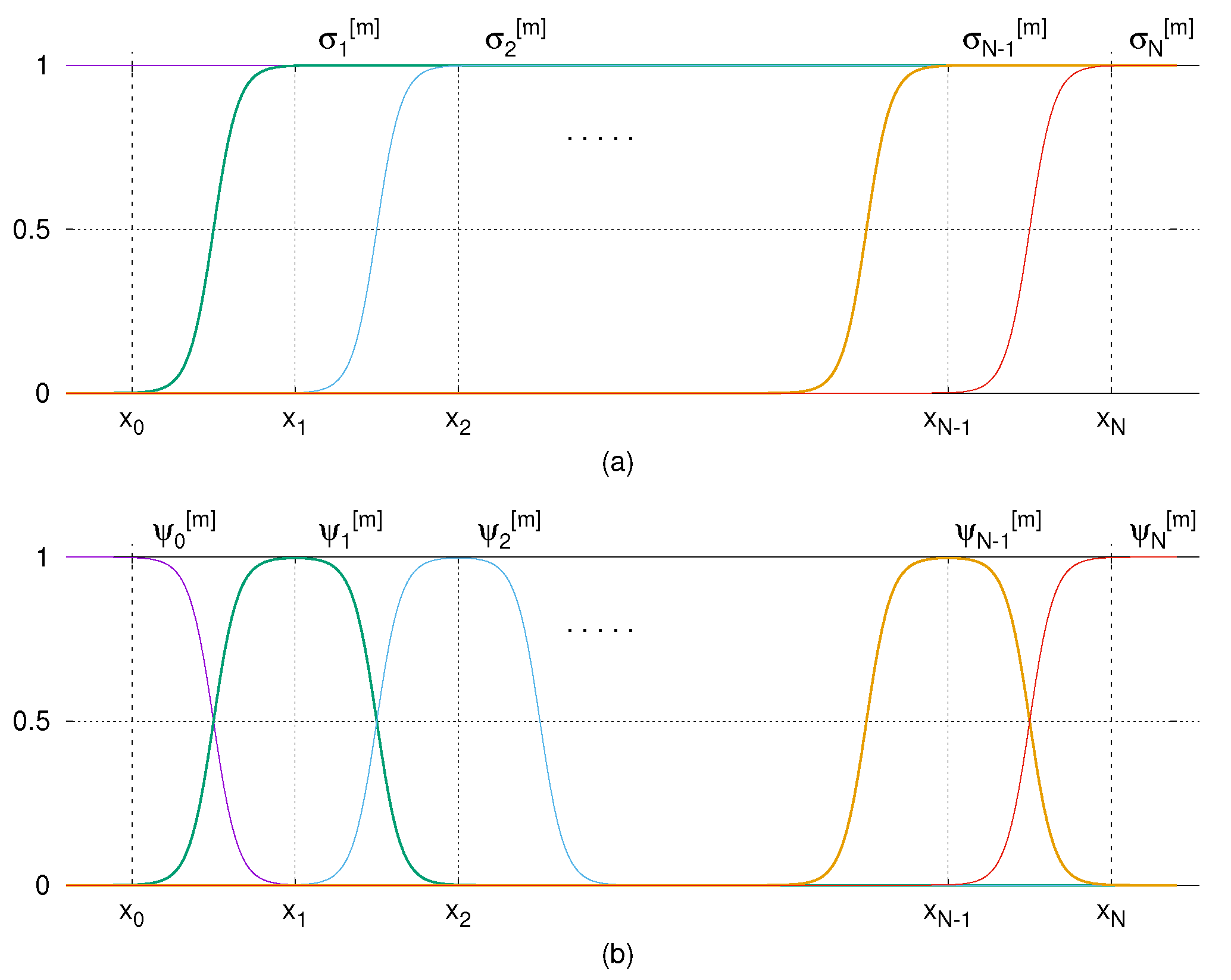
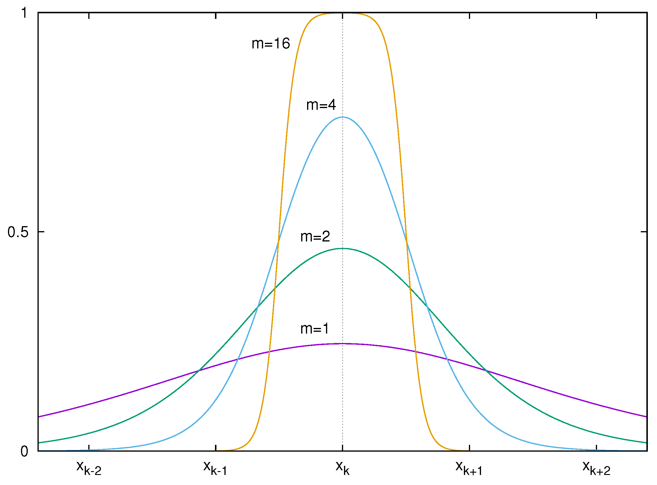
Graphs of the activation functions, and shown in Figure 1 illustrate the intuition of the construction of the presented quasi-interpolation . In addition, Figure 2 includes the graphs of with respect to the values , which shows that becomes flatter near the node and far from the node as the parameter m goes higher.
It is well known that the interpolants for continuous functions are guaranteed to be good if and only if the Lebesgue constants are small [15]. Regarding the formula (25) as an interpolation with equispaced points , its Lebesgue function satisfies
for all x, and thus the corresponding Lebesgue constant becomes . Noting that for the polynomial interpolation, the Lebesgue constant grows exponentially such as as , we may expect that will be better than the polynomial interpolation in approximation to any continuous function, at least.
4. Correction Formula
In order to improve the interpolation errors near the end-points of the given interval, that is, to make the formula (20) in Theorem 2 hold for all , we employ two values at the points and defined as
Using these additional data, we define a correction formula of (23) as
To explore the availability of the proposed approximation method (27), we consider the following examples which were employed in the literature [6].
Example 1.
A smooth function on the interval .
Example 2.
A function with jump-discontinuities.
We compare the results of the presented method with those of the existing neural network approximation method (5) using the activation function in (4). In the literature [6], it was proved that Theorem 1 holds if the weight is chosen such as
In practice, we have used in implementation of the existing FNN in (5) for the examples above. The high level software, Mathematica(V.10) has been used as a programming tool throughout the numerical performance for the examples.
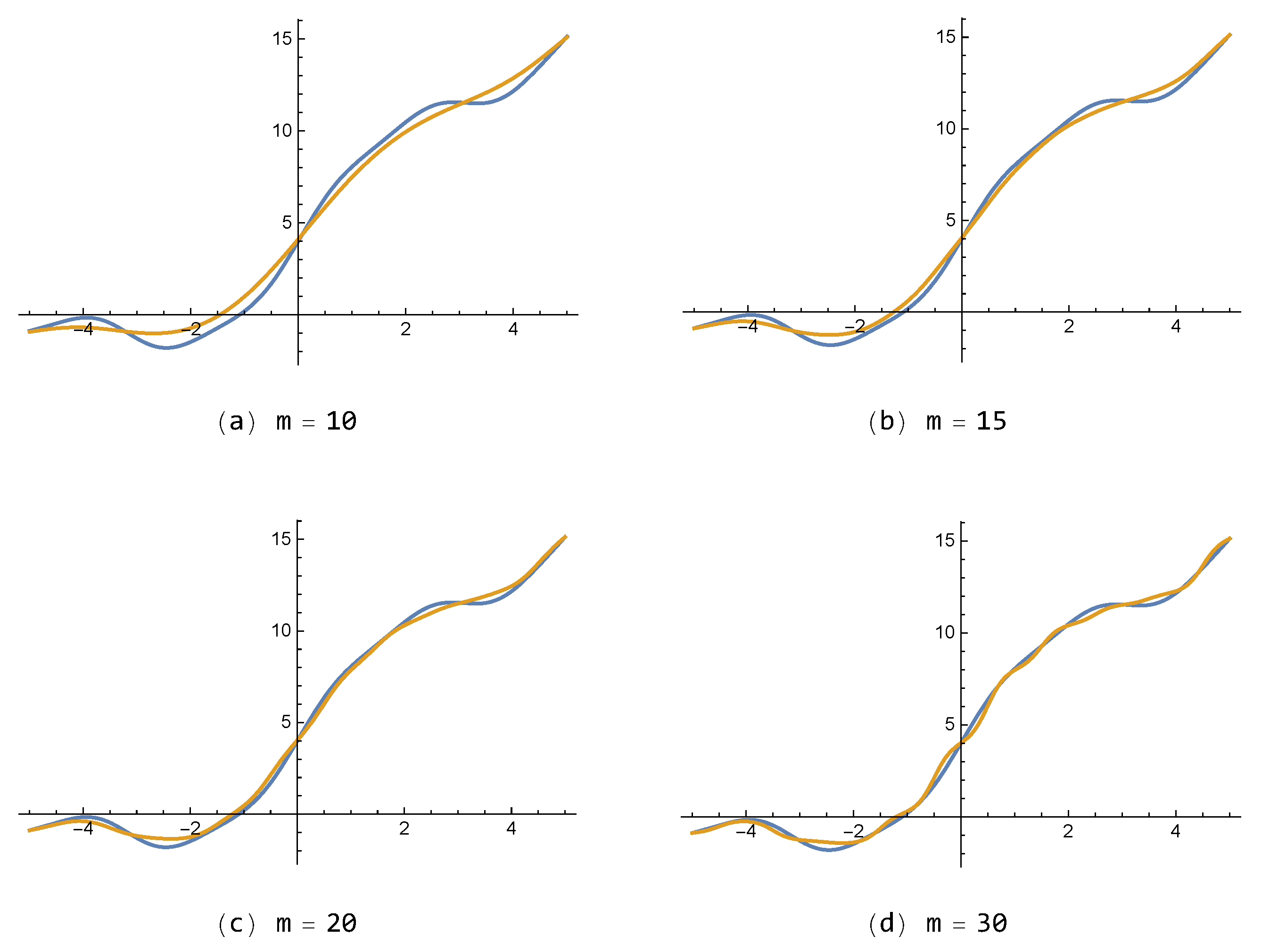
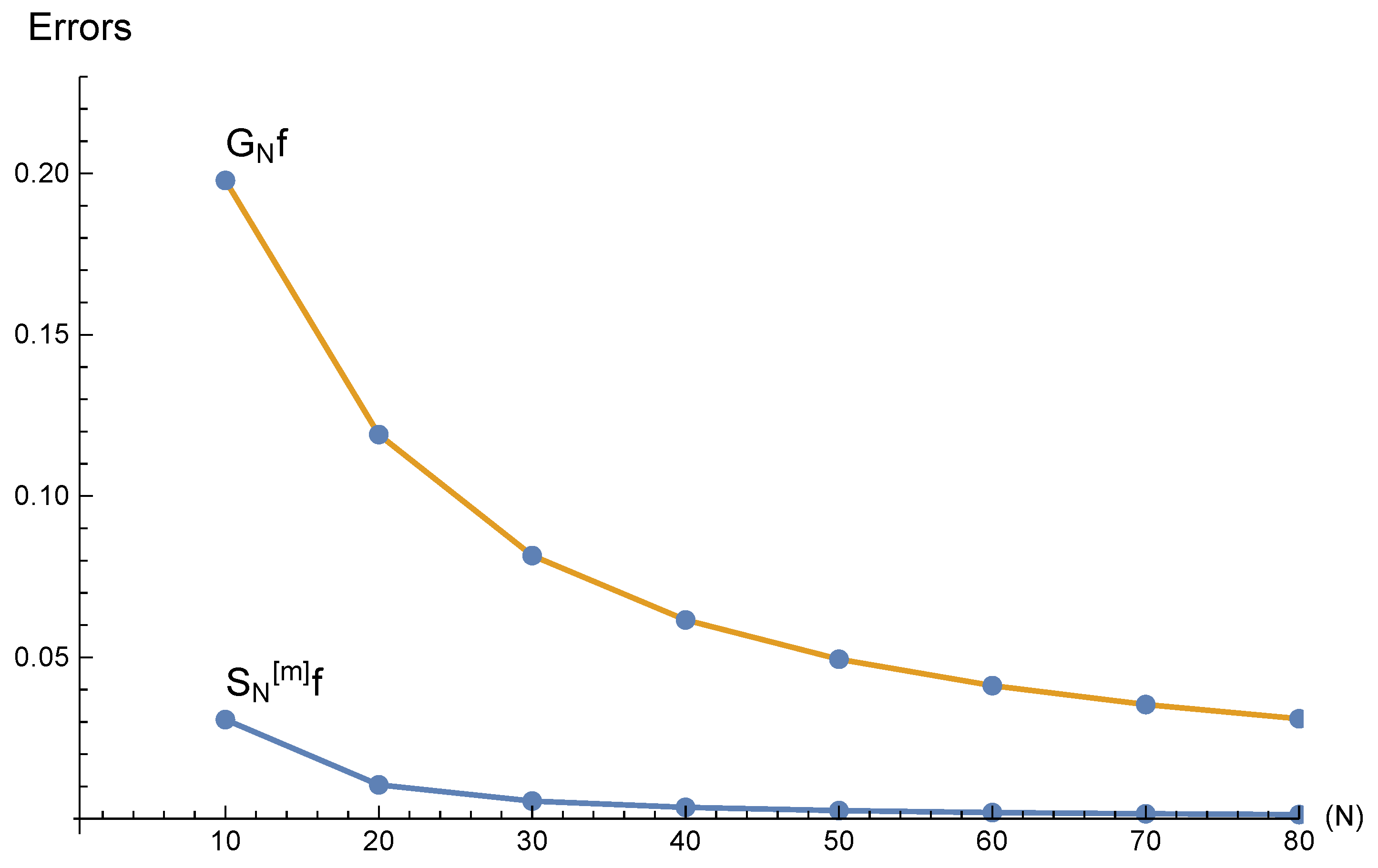
For the smooth function in Example 1, approximations of the proposed FNN , with small number of neurons () are shown in Figure 3 with respect to each parameter . The higher the value of m is, the more clearly reveals the so-called quasi-interpolation property as shown in Theorem 2. Moreover, Figure 4 shows errors of with , for the lower bound of m as given in (16), compared with errors of for . Therein the errors are defined as and . The figure illustrates that the presented FNN is superior to the existing FNN for continuous test function .
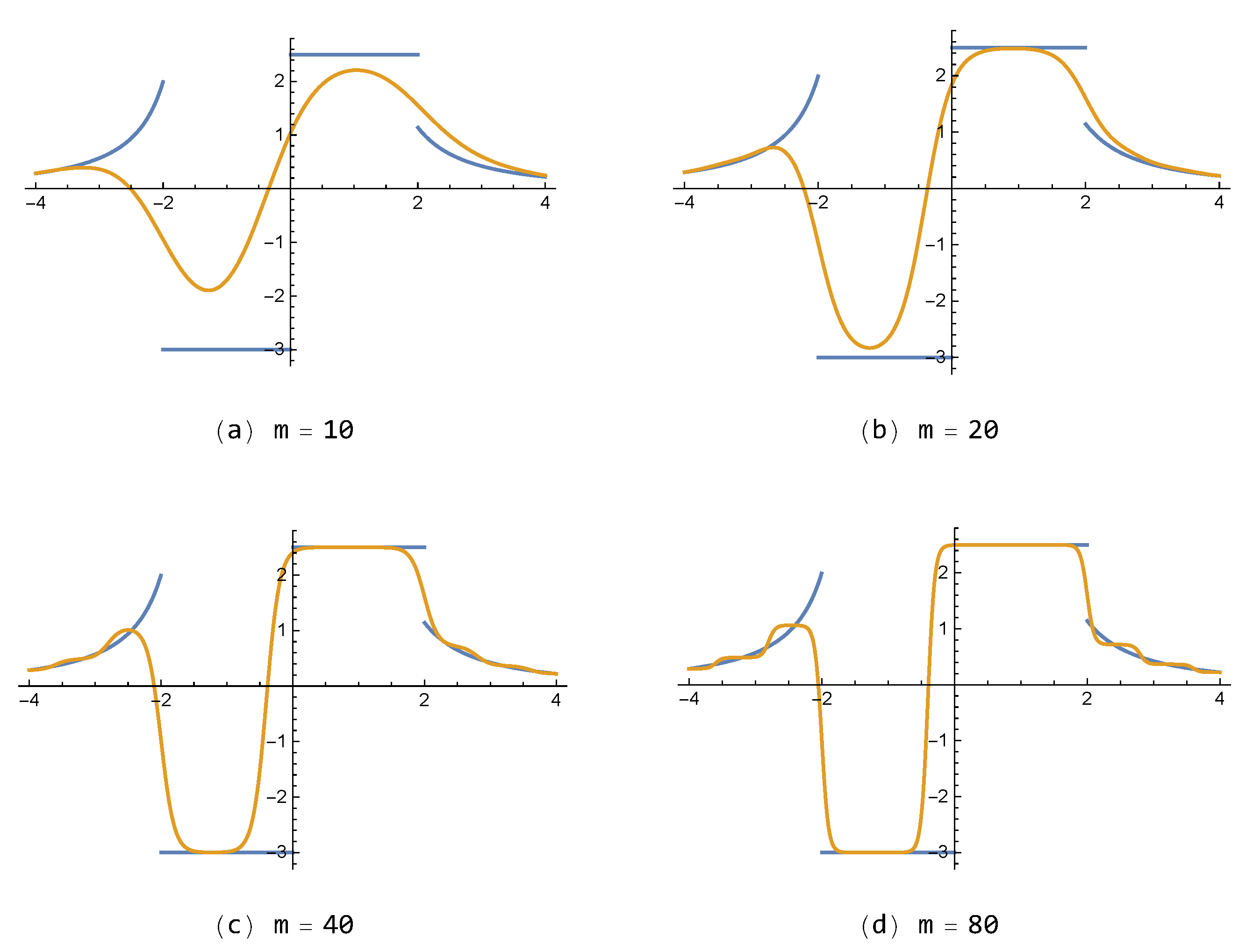
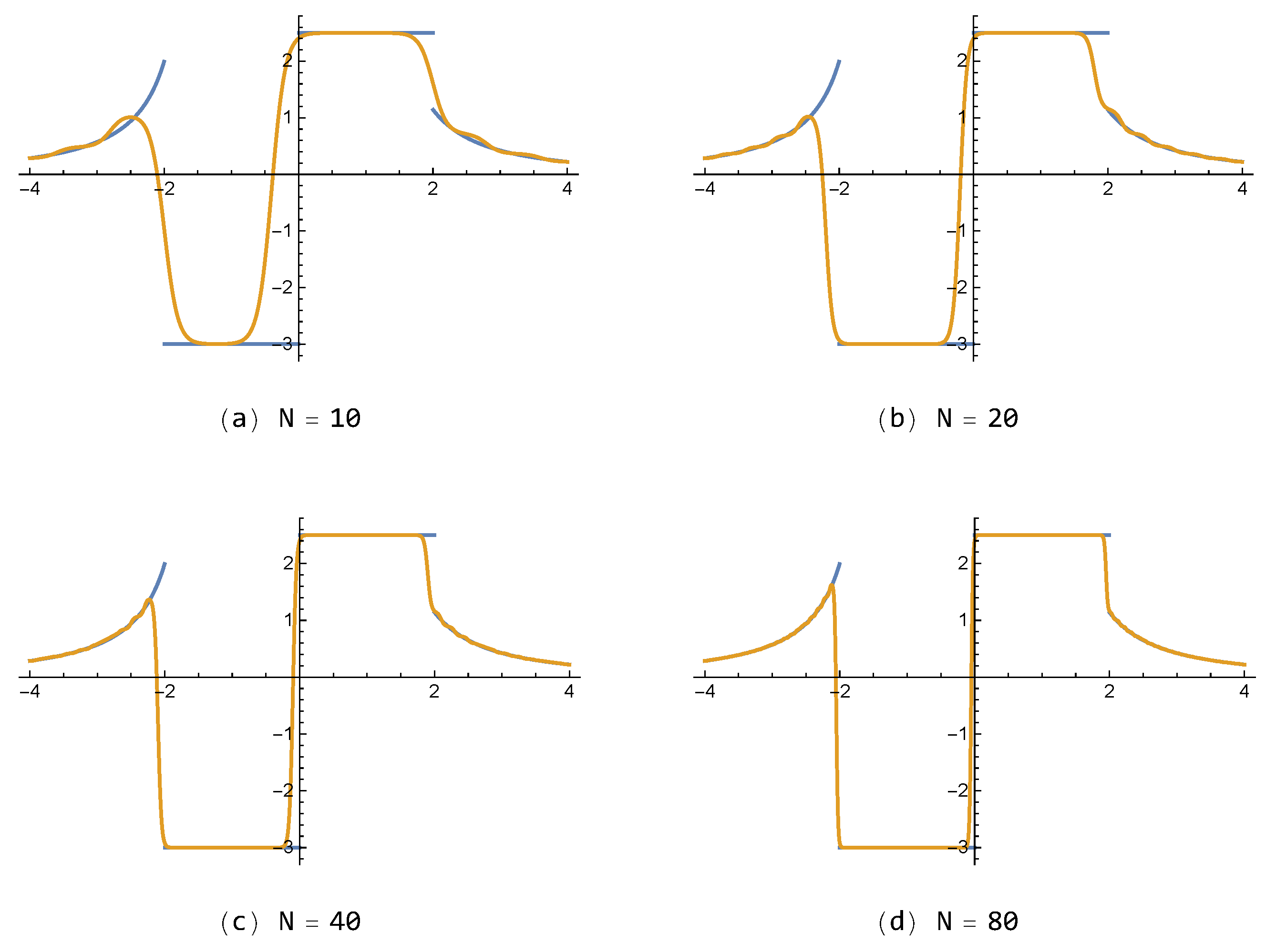
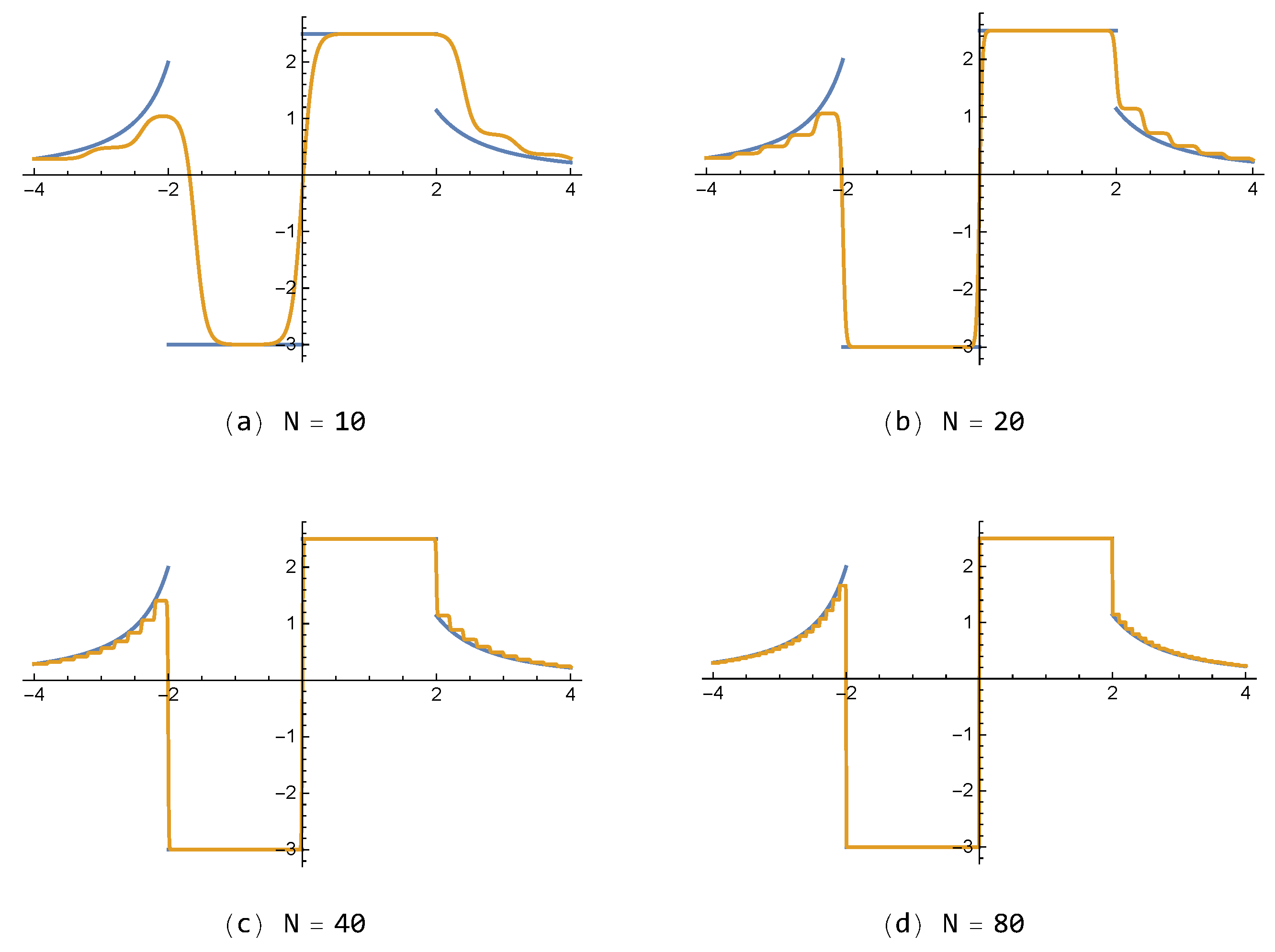
For the discontinuous function in Example 2, approximations of the proposed FNN , with small number of neurons (), are shown in Figure 5 with respect to each . In addition, approximations of for various values , with , are also given in Figure 6. One can see that the results of the presented method are better than those of shown in Figure 7. On the other hand, it is noted that the FNN approximations are free from the so-called Gibbs phenomenon, generating wiggles (i.e., overshoots and undershoots) near the jump-discontinuity, which appears inevitably in partial sum approximations composed of the polynomial or trigonometric base functions in general.
5. Multivariate Approximation
For simplicity we consider a function of two variables on a region , and assume that a set of data is given for the nodes
where , . Set activation functions
for , where ,
and is the parametric sigmoidal function in (6). Then, referring to the formula (25) under the assumption that m is large enough, we define an extended version of the FNN approximation to g as
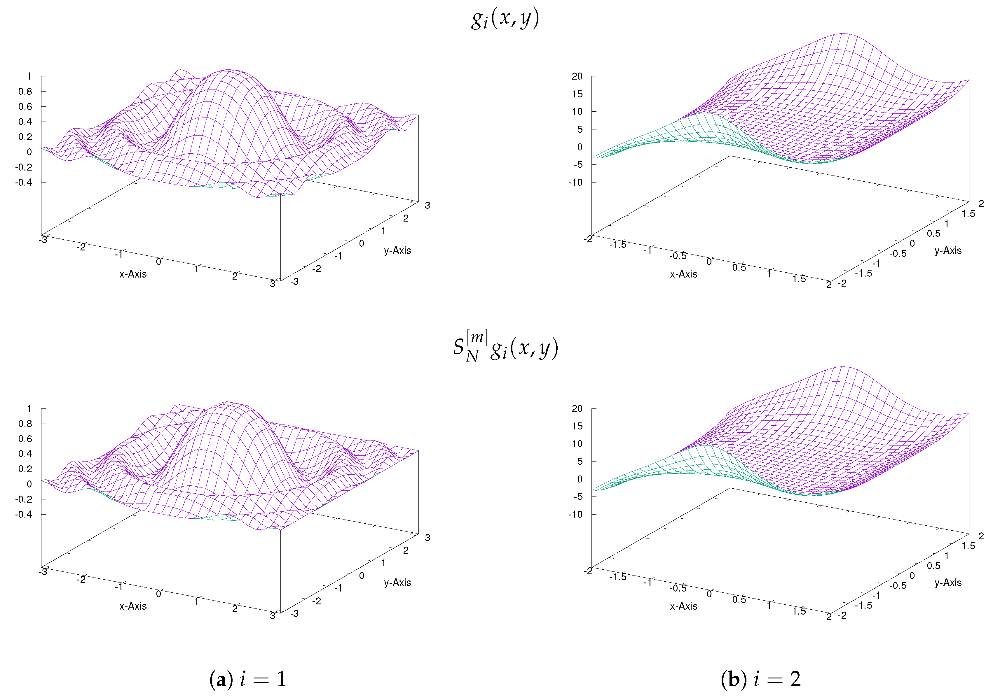
To testify the efficiency of the presented method (31), we choose functions of two variables below. In the numerical implementation for the examples the software, gnuplot(V.5) was used as it is rather fast for evaluating and graphing on two dimensional region.
Example 3.
Example 4.
6. Conclusions
In this work we proposed an FNN approximation method based on a new parametric sigmoidal activation function . It has been shown that the presented method with the parameter m large enough has a feature of the quasi-interpolation at the given nodes. As a result, we can note that the presented method is better than the existing FNN approximation method as demonstrated by the numerical results for several examples of univariate continuous and discontinuous functions. Additionally, the availability of the method in extended application to the multivariate function was illustrated.
Funding
This research was supported by Basic Science Research Program through the National Research Foundation of Korea (NRF) funded by the Ministry of Science and ICT (NRF-2017 R1A2B4007682).
Conflicts of Interest
The author declares no conflict of interest.
References
- Cybenko, G. Approximation by superpositions of a sigmoidal function. Math. Control Signal. 1989, 2, 303–314. [Google Scholar] [CrossRef]
- Funahashi, K.I. On the approximate realization of continuous mappings by neural networks. Neural Netw. 1989, 2, 183–192. [Google Scholar] [CrossRef]
- Hornik, K.; Stinchcombe, M.; White, H. Universal approximation of an unknown mapping and its derivatives using multilayer feedforward networs. Neural Netw. 1990, 3, 551–560. [Google Scholar] [CrossRef]
- Barron, A.R. Universal approximation bounds for superpositions of a sigmoidal function. IEEE Trans. Inform. Theory 1993, 39, 930–945. [Google Scholar] [CrossRef]
- Chen, Z.; Cao, F. The approximation operators with sigmoidal functions. Comput. Math. Appl. 2009, 58, 758–765. [Google Scholar] [CrossRef] [Green Version]
- Costarelli, D.; Spigler, R. Constructive approximation by superposition of sigmoidal functions. Anal. Theory Appl. 2013, 29, 169–196. [Google Scholar]
- Hahm, N.; Hong, B.I. An approximation by neural networks with a fixed weight. Compu.t Math. Appl. 2004, 47, 1897–1903. [Google Scholar] [CrossRef]
- Cao, F.L.; Xie, T.F.; Xu, Z.B. The estimate for approximation error of neural networks: A constructive approach. Neurocomputing 2008, 71, 626–630. [Google Scholar] [CrossRef]
- Chui, C.K.; Li, X. Approximation by ridge functions and neural networks with one hidden layer. J. Approx. Theory 1992, 70, 131–141. [Google Scholar] [CrossRef] [Green Version]
- Ferrari, S.; Stengel, R.F. Smooth Function Approximation Using Neural Networks. IEEE Trans. Neural Netw. 2005, 16, 24–38. [Google Scholar] [CrossRef] [PubMed] [Green Version]
- Suzuki, S. Constructive functions-approximation by three-layer artificial neural networks. Neural Netw. 1998, 11, 1049–1058. [Google Scholar] [CrossRef]
- Kyurkchiev, N.; Markov, S. Sigmoidal functions: Some computational and modelling aspects. Biomath Commun. 2014, 1. [Google Scholar] [CrossRef]
- Markov, S. Cell growth models using reaction schemes: Batch cultivation. Biomath 2013, 2. [Google Scholar] [CrossRef]
- Prössdorf, S.; Rathsfeld, A. On an integral equation of the first kind arising from a cruciform crack problem. In Integral Equations and Inverse Problems; Petkov, V., Lazarov, R., Eds.; Longman: Coventry, UK, 1991; pp. 210–219. [Google Scholar]
- Trefethen, L.N. Approximation Theory and Approximation Practice; SIAM: Oxford, UK, 2013; pp. 107–115. [Google Scholar]
- Yun, B.I. An extended sigmoidal transformation technique for evaluating weakly singular integrals without splitting the integration interval. SIAM J. Sci. Comput. 2003, 25, 284–301. [Google Scholar] [CrossRef]
- Yun, B.I. A smoothening method for the piecewise linear interpolation. J. Appl. Math. 2015, 2015, 376362. [Google Scholar] [CrossRef]
Figure 1.
Graphs of the sigmoidal functions in (a) and those of in (b).

Figure 2.
Graphs of for each , 2, 4, and 16.

Figure 3.
Approximations to by the presented feed-forward neural networks (FNN) with for each .

Figure 4.
Errors of the presented FNN approximations with and the existing FNN approximations for .

Figure 5.
Approximations to by the presented FNN with for each .

Figure 6.
Approximations to by the presented FNN for each with .

Figure 7.
Approximations to by the existing FNN for each .

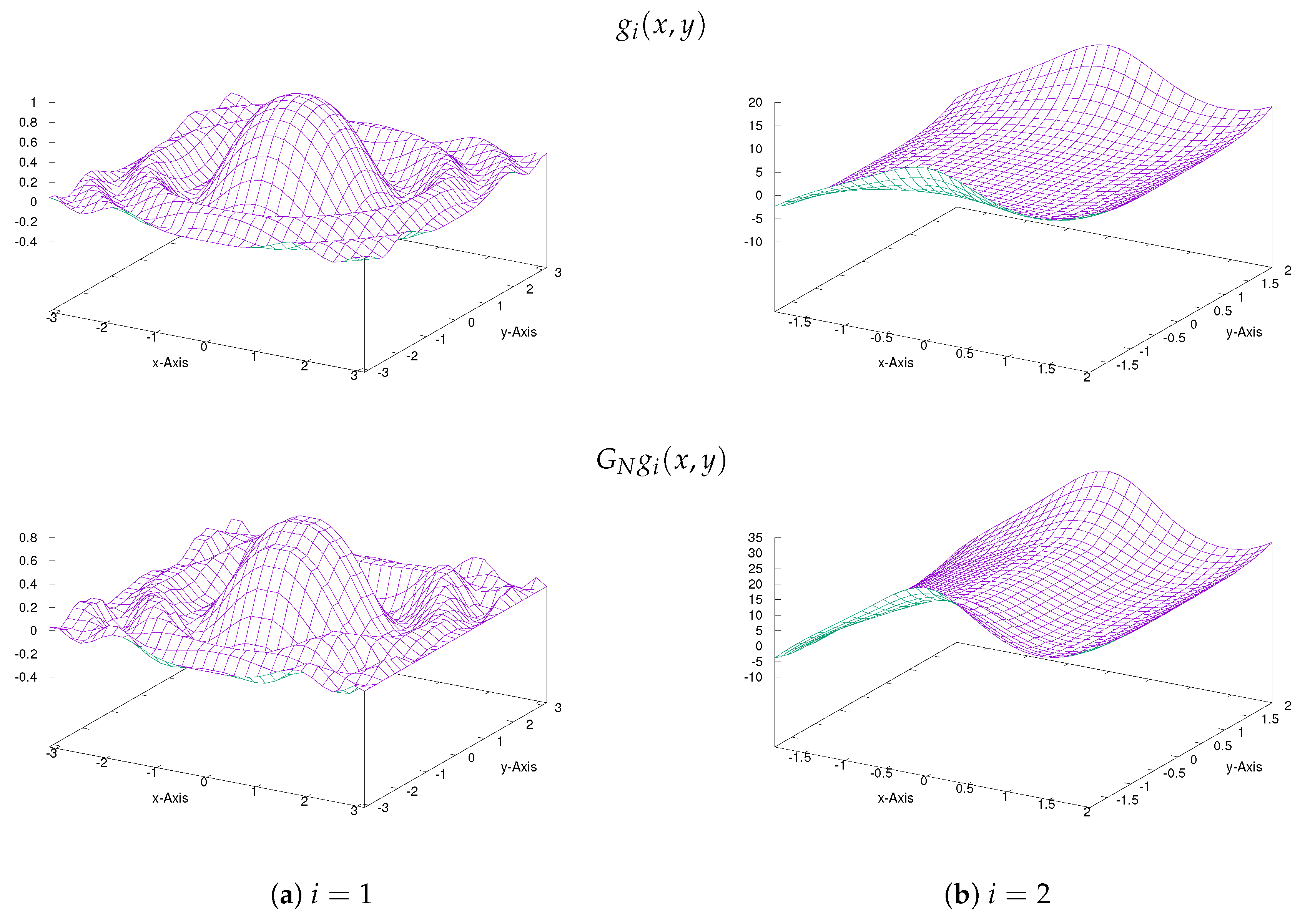
Figure 8.
Test functions (: upper row), , and their approximations by the presented FNN (: lower row) for with .
Figure 8.
Test functions (: upper row), , and their approximations by the presented FNN (: lower row) for with .

Figure 9.
Test functions (: upper row), , and their approximations by the existing FNN approximations (: lower row) for .
Figure 9.
Test functions (: upper row), , and their approximations by the existing FNN approximations (: lower row) for .

© 2019 by the author. Licensee MDPI, Basel, Switzerland. This article is an open access article distributed under the terms and conditions of the Creative Commons Attribution (CC BY) license (http://creativecommons.org/licenses/by/4.0/).
Share and Cite
MDPI and ACS Style
Yun, B.I. A Neural Network Approximation Based on a Parametric Sigmoidal Function. Mathematics 2019, 7, 262. https://0-doi-org.brum.beds.ac.uk/10.3390/math7030262
AMA Style
Yun BI. A Neural Network Approximation Based on a Parametric Sigmoidal Function. Mathematics. 2019; 7(3):262. https://0-doi-org.brum.beds.ac.uk/10.3390/math7030262
Chicago/Turabian StyleYun, Beong In. 2019. "A Neural Network Approximation Based on a Parametric Sigmoidal Function" Mathematics 7, no. 3: 262. https://0-doi-org.brum.beds.ac.uk/10.3390/math7030262
Note that from the first issue of 2016, this journal uses article numbers instead of page numbers. See further details here.