Homogeneous Groups of Actors in an AHP-Local Decision Making Context: A Bayesian Analysis

Abstract

The two procedures traditionally followed for group decision making with the Analytical Hierarchical Process (AHP) are the Aggregation of Individual Judgments (AIJ) and the Aggregation of Individual Priorities (AIP). In both cases, the geometric mean is used to synthesise judgments and individual priorities into a collective position. Unfortunately, positional measures (means) are only representative if dispersion is reduced. It is therefore necessary to develop decision tools that allow: (i) the identification of groups of actors that present homogeneous and differentiated behaviours; and, (ii) the aggregation of the priorities of the near groups to reach collective positions with the greatest possible consensus. Following a Bayesian approach to AHP in a local context (a single criterion), this work proposes a methodology to solve these problems when the number of actors is not high. The method is based on Bayesian comparison and selection of model tools which identify the number and composition of the groups as well as their priorities. This information can be very useful to identify agreement paths among the decision makers that can culminate in a more representative decision-making process. The proposal is illustrated by a real-life case study.

1. Introduction

Two of the most outstanding characteristics of the Knowledge Society (KS), understood as a space for the talent, imagination and creativity of human beings, are [1]: (i) the collaborative predisposition of citizens in the resolution of complex problems, motivated by the existence of a more educated and participative society that wants to be involved in decision-making processes; and, (ii) the relevance of the human factor and the need for the formal models to incorporate the subjective, intangible and emotional aspects inherent to the human being, alongside the tangible and rational objectives of the traditional scientific method.

In order to take advantage of the characteristics of the KS and to provide an adequate response to new challenges and needs, it is necessary to develop appropriate analytical and computing decision-making tools to solve the complex problems characterised by the existence of multiple scenarios, actors and both tangible and intangible criteria. One of the most utilised multicriteria techniques that best incorporates intangible aspects and multiple actors is the Analytic Hierarchy Process (AHP) proposed by Thomas L. Saaty in the mid-1970s [2]. The methodology consists of three stages: (i) Hierarchical modelling; (ii) Valuation; (iii) Prioritisation and Synthesis.

AHP incorporates the intangible through the judgments issued when assessing the matrices of paired comparisons considered in the problem. The two most commonly used methods in AHP for the calculus of collective priorities in multi-actor decision making are [3,4,5]: the Aggregation of Individual Judgments (AIJ) and the Aggregation of Individual Priorities (AIP). They obtain, as averages (geometric mean), the collective judgments or collective priorities. The average is not a representative indicator of the collective when it is not homogeneous. It is therefore necessary to evaluate the compatibility (an objective measure obtained automatically) or the agreement (a subjective measure that requires personal intervention) between the individual positions of the actors and the position of the group.

If not all actors are compatible with the collective priority vector, the different positions and the actors that support them must be identified in order to initiate posterior negotiation processes to achieve final decisions that are as representative as possible. This paper presents a Bayesian procedure to solve this problem in a local context (a single criterion). The procedure adopts the Bayesian hierarchical approach (Stochastic AHP) proposed in reference [6]. It allows the estimation of the priorities of the group by incorporating restrictions on the maximum level of inconsistency of the actors involved in the problem. The procedure quantifies the homogeneity of the groups by means of the marginal density of the judgments elicited by their respective actors. The density evaluates the goodness of fit of the model and allows for comparisons between different partitions of the set of actors. The work further puts forward an algorithm for the exhaustive search of homogeneous groups with respect to their priorities based on the Bayesian comparison and selection of models. The methodology is illustrated by a practical example.

The paper is structured as follows: Section 2 presents the model used to determine the priorities of a group of homogeneous decision makers; Section 3 describes the algorithm that identifies decision groups with homogeneous preferences; Section 4 applies the methodology to a case study; and, Section 5 concludes by highlighting the most relevant aspects of the work and possible extensions.

2. Bayesian Local Priorities in an AHP-Multi-Actor Decision Making Context

This section deals with the problem of determining the total priorities of a group of actors with homogeneous opinions regarding a decision criterion. A Bayesian statistical approach based on the use of a log-linear model similar to that used in reference [6] is employed to describe the process of the issuing judgments by the decision makers of a group. The posterior distribution of the group’s priorities is calculated by means of Bayes’ Theorem; this is followed by a description of how to make inferences about the most preferred alternative (alpha problem—P.α) and the priority ranking (gamma problem—P.γ).

2.1. Problem Formulation

First, the log-linear model that is used to determine the priorities of the groups of decision makers is explained: in what follows, N (µ, σ) denotes the univariate normal distribution of mean µ and standard deviation σ; N_p (µ, ∑) denotes the p-variant normal distribution of mean vector µ and the matrix of variances and covariances ∑; T_p (µ, ∑, υ) denotes the p-variant Student t distribution with mean vector µ, scale matrix ∑ and degrees of freedom υ; Gamma(p, a) denotes the gamma distribution with shape parameter p and scale parameter 1/a; ${\mathrm{\chi }}_{\mathrm{\nu }}^2$ denotes the chi-squared distribution with υ degrees of freedom; I_A denotes the indicator function of set A; ∝ indicates ‘proportional to’ and [Y|X] denotes the density function of the conditional distribution of Y given X.

Let G = {D^[1],…., D^[K]} be a group of K homogeneous decision makers (k = 1, …, K), A = {A₁,…, A_n} be a set of n alternatives and R^(k) = $\left({\mathrm{r}}_{\mathrm{i}\mathrm{j}}^{(\mathrm{k})}\right)$; k = 1,…, K be the nxn paired comparison matrices issued by each decision maker.

We assume, without loss of generality, that the matrices of judgments are complete—all paired comparisons have been made. If some of the r_ij comparisons are missing, the proposed methodology could be analogously adapted, as shown in reference [6].

We further assume that the decision makers of G have homogeneous opinions regarding the priorities of each of the alternatives of A so that:

$${\mathrm{y}}_{\mathrm{i}\mathrm{j}}^{(\mathrm{k})}={\mathsf{\mu }}_{\mathrm{i}}^{(\mathrm{G})}-{\mathsf{\mu }}_{\mathrm{j}}^{(\mathrm{G})}+{\mathsf{\epsilon }}_{\mathrm{i}\mathrm{j}}^{(\mathrm{k})};\mathrm{k}=1,\dots ,\mathrm{K};1\le \mathrm{i}<\mathrm{j}\le \mathrm{n};$$

(1)

with ${\mathrm{y}}_{\mathrm{i}\mathrm{j}}^{(\mathrm{k})}=\log \left({\mathrm{r}}_{\mathrm{i}\mathrm{j}}^{(\mathrm{k})}\right)$, where:

(a)

${\mathsf{\mu }}_{\mathrm{i}}^{\left(\mathrm{G}\right)}=\log \left({\mathrm{v}}_{\mathrm{i}}^{\left(\mathrm{G}\right)}\right)$; i = 1, …, n being ${\mathrm{v}}_{\mathrm{i}}^{\left(\mathrm{G}\right)}$ the priority (without normalising) given to the alternative A_i by the members of the group G

(b)

${\mathrm{v}}_{\mathrm{n}}^{\left(\mathrm{G}\right)}=1$ (that is to say, ${\mathsf{\mu }}_{\mathrm{n}}^{\left(\mathrm{G}\right)}=0$) to avoid identifiability problems

(c)

${\mathsf{\epsilon }}_{\mathrm{i}\mathrm{j}}^{(\mathrm{k})}~\mathrm{N}\left(0,{\mathsf{\sigma }}^{(\mathrm{G})}\right)$; k = 1, …, K; 1 ≤ i < j ≤ n independents

The normalised priorities of the group will be given by the vector $w^{(\mathrm{G})}={\left({\mathrm{w}}_{\mathrm{i}}^{\left(\mathrm{G}\right)};\mathrm{i}=1,\dots ,\mathrm{n}\right)}^{\prime }$ where ${\mathrm{w}}_{\mathrm{i}}^{\left(\mathrm{G}\right)}=\frac{{\mathrm{v}}_{\mathrm{i}}^{\left(\mathrm{G}\right)}}{{\displaystyle \sum _{\mathrm{i}=1}^{\mathrm{n}}{\mathrm{v}}_{\mathrm{i}}^{\left(\mathrm{G}\right)}}}$; i = 1, …, n. Likewise, the level of homogeneity will be determined by the standard deviation of the errors σ^(G) that quantifies the inconsistency level of all decision makers in the group with the priority vector w^(G).

2.2. Estimation of the Local Priorities for the Group

The estimation of the vector of group priorities w^(G) uses a Bayesian approach that allows exact inferences about their values. We adopt, as a prior, a normal-gamma distribution given by:

$${\mathsf{\mu }}^{\left(\mathrm{G}\right)}={\left({\mathsf{\mu }}_1^{\left(\mathrm{G}\right)},\dots ,{\mathsf{\mu }}_{\mathrm{n}-1}^{\left(\mathrm{G}\right)}\right)}^{\prime }|{\mathsf{\tau }}^{(\mathrm{G})}~{\mathrm{N}}_{\mathrm{n}-1}\left(0,\frac{1}{{\mathrm{c}}_0{\mathsf{\tau }}^{(\mathrm{G})}}{I}_{\mathrm{n}-1}\right)\mathrm{with}{\mathrm{c}}_0>0$$

(2)

$${\mathsf{\tau }}^{(\mathrm{G})}=\frac{1}{{\mathsf{\sigma }}^{\left(\mathrm{G}\right)2}}~\mathrm{G}\mathrm{a}\mathrm{m}\mathrm{m}\mathrm{a}\left(\frac{{\mathrm{n}}_0}{2},\frac{{\mathrm{n}}_0{\mathrm{s}}_0^2}{2}\right)$$

(3)

that is the standard conjugate distribution used in Bayesian literature [7]. The constants c₀, n₀ and ${\mathrm{s}}_0^2$ determine the degree of strength of the prior distribution. In the illustrative example we have taken c₀ = 0.1 so that the influence of the prior distribution of µ^(G) is not significant. The hyper-parameters n₀ and ${\mathrm{s}}_0^2$ are determined from the maximum levels of inconsistency ${\mathsf{\sigma }}_{\max }^2$ allowed for each decision maker so that

$$\mathrm{P}\left[0\le {\mathsf{\sigma }}^{\left(\mathrm{G}\right)2}\le {\mathsf{\sigma }}_{\max }^2\right]=1-\mathsf{\alpha }$$

being, 1 − α (0 < α < 1) the level of credibility that we want to achieve. The value of ${\mathsf{\sigma }}_{\max }^2$ has been set using the consistency thresholds of the geometric consistency index (GCI) proposed by [8]. In our illustrative example, and given that n = 4, we take ${\mathsf{\sigma }}_{\max }^2$ = 0.35 and α = 0.05, which resulted in n₀ = 0.1 and ${\mathrm{s}}_0^2$ = 0.0014.

Using Bayes’ theorem, and taking into account (1)–(3), we calculate the posterior distribution of (µ^(G), τ^(G)) whose density is given by:

$$\begin{array}{c}\left[{\mathsf{\mu }}^{\left(\mathrm{G}\right)}|{\mathsf{\tau }}^{(\mathrm{G})},\left\{y^{(\mathrm{k})};\mathrm{k}\in \left\{1,\dots ,\mathrm{K}\right\}\right\}\right]\propto {\displaystyle \prod _{1\le \mathrm{i}<\mathrm{j}\le \mathrm{n}}^{}\left[{\mathrm{y}}_{\mathrm{i}\mathrm{j}}^{(\mathrm{k})}|{\mathsf{\mu }}^{\left(\mathrm{G}\right)},{\mathsf{\tau }}^{\left(\mathrm{G}\right)}\right]}\left[{\mathsf{\mu }}^{\left(\mathrm{G}\right)}|{\mathsf{\tau }}^{(\mathrm{G})}\right]\left[{\mathsf{\tau }}^{(\mathrm{G})}\right]\propto \\ \propto {\displaystyle \prod _{\mathrm{k}=1}^{\mathrm{K}}{\displaystyle \prod _{1\le \mathrm{i}<\mathrm{j}\le \mathrm{n}}{\left({\mathsf{\tau }}^{\left(\mathrm{G}\right)}\right)}^{\frac{1}{2}}\exp \left[-\frac{{\mathsf{\tau }}^{\left(\mathrm{G}\right)}}{2}{\left({\mathrm{y}}_{\mathrm{i}\mathrm{j}}^{(\mathrm{k})}-{\mathsf{\mu }}_{\mathrm{i}}^{\left(\mathrm{G}\right)}+{\mathsf{\mu }}_{\mathrm{j}}^{\left(\mathrm{G}\right)}\right)}^2\right]}}{\left({\mathsf{\tau }}^{\left(\mathrm{G}\right)}\right)}^{\frac{\mathrm{n}-1}{2}}\exp \left[-\frac{{\mathrm{c}}_0{\mathsf{\tau }}^{\left(\mathrm{G}\right)}}{2}\left({\displaystyle \sum _{\mathrm{i}=1}^{\mathrm{n}-1}{\left({\mathsf{\mu }}_{\mathrm{i}}^{\left(\mathrm{G}\right)}\right)}^2}\right)\right]\\ \mathrm{x}{\left({\mathsf{\tau }}^{\left(\mathrm{G}\right)}\right)}^{\frac{{\mathrm{n}}_0}{2}-1}\exp \left[-\frac{{\mathsf{\tau }}^{\left(\mathrm{G}\right)}}{2}{\mathrm{n}}_0{\mathrm{s}}_0^2\right]{\mathrm{I}}_{\left(0,\infty \right)}\left({\mathsf{\tau }}^{\left(\mathrm{G}\right)}\right)=\\ ={\left({\mathsf{\tau }}^{\left(\mathrm{G}\right)}\right)}^{\frac{\mathrm{J}\mathrm{K}+\mathrm{n}-1+{\mathrm{n}}_0}{2}-1}\exp \left[-\frac{{\mathsf{\tau }}^{\left(\mathrm{G}\right)}}{2}\left[{\mathrm{n}}_0{\mathrm{s}}_0^2+{\displaystyle \sum _{\mathrm{k}=1}^{\mathrm{K}}{\displaystyle \sum _{1\le \mathrm{i}<\mathrm{j}\le \mathrm{n}}{\left({\mathrm{y}}_{\mathrm{i}\mathrm{j}}^{(\mathrm{k})}-{\mathsf{\mu }}_{\mathrm{i}}^{\left(\mathrm{G}\right)}+{\mathsf{\mu }}_{\mathrm{j}}^{\left(\mathrm{G}\right)}\right)}^2}}+{\mathrm{c}}_0\left({\displaystyle \sum _{\mathrm{i}=1}^{\mathrm{n}-1}{\left({\mathsf{\mu }}_{\mathrm{i}}^{\left(\mathrm{G}\right)}\right)}^2}\right)\right]\right]{\mathrm{I}}_{\left(0,\infty \right)}\left({\mathsf{\tau }}^{\left(\mathrm{G}\right)}\right)\\ ={\left({\mathsf{\tau }}^{\left(\mathrm{G}\right)}\right)}^{{}^{\frac{\mathrm{J}\mathrm{K}+\mathrm{n}-1+{\mathrm{n}}_0}{2}-1}}\exp \left[-\frac{{\mathsf{\tau }}^{\left(\mathrm{G}\right)}}{2}\left[{\mathrm{n}}_0{\mathrm{s}}_0^2+{\displaystyle \sum _{\mathrm{k}=1}^{\mathrm{K}}{\left(y^{(\mathrm{k})}-X{\mathsf{\mu }}^{\left(\mathrm{G}\right)}\right)}^{\prime }\left(y^{(\mathrm{k})}-X{\mathsf{\mu }}^{\left(\mathrm{G}\right)}\right)}+{\mathrm{c}}_0\left({\mathsf{\mu }}^{\left(\mathrm{G}\right)\prime }{\mathsf{\mu }}^{\left(\mathrm{G}\right)}\right)\right]\right]{\mathrm{I}}_{\left(0,\infty \right)}\left({\mathsf{\tau }}^{\left(\mathrm{G}\right)}\right)\end{array}$$

(4)

where $y^{(\mathrm{k})}={\left({\mathrm{y}}_{\mathrm{i}\mathrm{j}}^{(\mathrm{k})};1\le \mathrm{i}<\mathrm{j}\le \mathrm{n}\right)}^{\prime }$ for k = 1, …, K and X = (x_ij) (J × (n − 1)) with $\mathrm{J}=\frac{\mathrm{n}(\mathrm{n}-1)}{2}$ is the regression matrix of model (1) so that:

-

x_ij = 1 if the ith judgement is y_jk with k ≠ j;

-

x_ij = −1 if the ith judgement is y_kj with k ≠ j;

-

x_ij = 0 in any other case.

It follows that:

$$\begin{array}{c}\left[{\mathsf{\mu }}^{\left(\mathrm{G}\right)}|{\mathsf{\tau }}^{(\mathrm{G})},\left\{y^{(\mathrm{k})};\mathrm{k}\in \left\{1,\dots ,\mathrm{K}\right\}\right\}\right]\propto \\ \propto {\left({\mathsf{\tau }}^{\left(\mathrm{G}\right)}\right)}^{\frac{\mathrm{J}\mathrm{K}+{\mathrm{n}}_0}{2}-1}\exp \left[-\frac{{\mathsf{\tau }}^{\left(\mathrm{G}\right)}}{2}\left\{{\mathrm{n}}_0{\mathrm{s}}_0^2+{\displaystyle \sum _{\mathrm{k}=1}^{\mathrm{K}}{y}^{(\mathrm{k})\prime }{y}^{(\mathrm{k})}}-m^{\left(\mathrm{g}\right)\prime }\left(\mathrm{K}\left(X^{\prime }X\right)+{\mathrm{c}}_0{\mathrm{I}}_{\mathrm{n}-1}\right)m^{\left(\mathrm{g}\right)}\right\}\right]\mathrm{x}\\ \mathrm{x}{\left({\mathsf{\tau }}^{\left(\mathrm{G}\right)}\right)}^{\frac{\mathrm{n}-1}{2}-1}\exp \left[-\frac{{\mathsf{\tau }}^{\left(\mathrm{G}\right)}}{2}\left\{{\left({\mathsf{\mu }}^{\left(\mathrm{G}\right)}-m^{\left(\mathrm{G}\right)}\right)}^{\prime }\left(\mathrm{K}\left(X^{\prime }X\right)+{\mathrm{c}}_0{\mathrm{I}}_{\mathrm{n}-1}\right)\left({\mathsf{\mu }}^{\left(\mathrm{G}\right)}-m^{\left(\mathrm{G}\right)}\right)\right\}\right]{\mathrm{I}}_{\left(0,\infty \right)}\left({\mathsf{\tau }}^{\left(\mathrm{G}\right)}\right)\end{array}$$

(5)

where $m^{(\mathrm{G})}={\left(\mathrm{K}\left(X^{\prime }X\right)+{\mathrm{c}}_0{\mathrm{I}}_{\mathrm{n}-1}\right)}^{-1}\left(X^{\prime }\left({\displaystyle \sum _{\mathrm{k}=1}^{\mathrm{K}}{y}^{(\mathrm{k})}}\right)\right)$.

Therefore, it follows from (5) that:

$${\mathsf{\mu }}^{\left(\mathrm{G}\right)}|{\mathsf{\tau }}^{(\mathrm{G})},\left\{y^{(\mathrm{k})};\mathrm{k}\in \left\{1,\dots ,\mathrm{K}\right\}\right\}~{\mathrm{N}}_{\mathrm{n}-1}\left(m^{\left(\mathrm{G}\right)},\frac{1}{{\mathsf{\tau }}^{\left(\mathrm{G}\right)}}{\left(\mathrm{K}\left(X^{\prime }X\right)+{\mathrm{c}}_0{\mathrm{I}}_{\mathrm{n}-1}\right)}^{-1}\right)$$

(6)

$${\mathsf{\tau }}^{(\mathrm{G})}|\left\{y^{(\mathrm{k})};\mathrm{k}\in \left\{1,\dots ,\mathrm{K}\right\}\right\}~\mathrm{G}\mathrm{a}\mathrm{m}\mathrm{m}\mathrm{a}\left(\frac{{\mathrm{n}}_0+\mathrm{J}\mathrm{K}}{2},\left(\frac{{\mathrm{n}}_0+\mathrm{J}\mathrm{K}}{2}\right){\mathrm{s}}^{\left(\mathrm{G}\right)2}\right)$$

(7)

where ${\mathrm{s}}^{2(\mathrm{G})}=\frac{{\mathrm{n}}_0{\mathrm{s}}_0^2+{\displaystyle \sum _{\mathrm{k}=1}^{\mathrm{K}}{y}^{(\mathrm{k})\prime }{y}^{(\mathrm{k})}}-m^{\left(\mathrm{G}\right)\prime }\left(\mathrm{K}\left(X^{\prime }X\right)+{\mathrm{c}}_0{\mathrm{I}}_{\mathrm{n}-1}\right)m^{\left(\mathrm{G}\right)}}{{\mathrm{n}}_0+\mathrm{J}\mathrm{K}}$.

Integrating with respect to τ^(G) in (5), it follows that:

$${\mathsf{\mu }}^{\left(\mathrm{G}\right)}|\left\{y^{(\mathrm{k})};\mathrm{k}\in \left\{1,\dots ,\mathrm{K}\right\}\right\}~{\mathrm{T}}_{\mathrm{n}-1}\left(m^{\left(\mathrm{G}\right)},{\mathrm{s}}^{\left(\mathrm{G}\right)2}{\left(\mathrm{K}\left(X^{\prime }X\right)+{\mathrm{c}}_0{\mathrm{I}}_{\mathrm{n}-1}\right)}^{-1},{\mathrm{n}}_0+\mathrm{J}\mathrm{K}\right)$$

(8)

From the posterior distributions (7) and (8), point estimates and credibility intervals of w^(G) and σ^(G) can be obtained using the posterior median and the corresponding quantiles.

In the case of σ^2(G), and taking into account that from (7) ${\mathsf{\tau }}^{(\mathrm{G})}~\frac{{\mathsf{\chi }}_{{\mathrm{n}}_0+\mathrm{J}\mathrm{K}}^2}{\left({\mathrm{n}}_0+\mathrm{J}\mathrm{K}\right){\mathrm{s}}^{\left(\mathrm{G}\right)2}}$, a 100 (1 − α)%, the Bayesian credibility interval for σ^2(G) is given by $\left[\frac{{\mathrm{s}}^{2\left(\mathrm{G}\right)}\left({\mathrm{n}}_0+\mathrm{J}\mathrm{K}\right)}{{\mathsf{\chi }}_{{\mathrm{n}}_0+\mathrm{J}\mathrm{K},1-\frac{\mathsf{\alpha }}{2}}^2},\frac{{\mathrm{s}}^{2\left(\mathrm{G}\right)}\left({\mathrm{n}}_0+\mathrm{J}\mathrm{K}\right)}{{\mathsf{\chi }}_{{\mathrm{n}}_0+\mathrm{J}\mathrm{K},\frac{\mathsf{\alpha }}{2}}^2}\right]$ where ${\mathsf{\chi }}_{\mathsf{\nu },\mathsf{\alpha }}^2$ denotes the (1 − α)th quantile of the distribution ${\mathsf{\chi }}_{\mathsf{\nu }}^2$.

To calculate a credibility interval for ${\mathrm{w}}_{\mathrm{i}}^{(\mathrm{G})}$ (1 ≤ i ≤ n) the Monte Carlo method is applied by extracting a sample $\left\{{\mathsf{\mu }}_{}^{(\mathrm{G},\mathrm{s})}={\left({\mathsf{\mu }}_1^{(\mathrm{G},\mathrm{s})},\dots ,{\mathsf{\mu }}_{\mathrm{n}-1}^{(\mathrm{G},\mathrm{s})}\right)}^{\prime };\mathrm{s}=1,\dots ,\mathrm{S}\right\}$ from (8) and calculating a sample of the posterior distribution of w^(G), $W^{(\mathrm{G})}=\left\{w_{}^{(\mathrm{G},\mathrm{s})}={\left({\mathrm{w}}_1^{(\mathrm{G},\mathrm{s})},\dots ,{\mathrm{w}}_{\mathrm{n}}^{(\mathrm{G},\mathrm{s})}\right)}^{\prime };\mathrm{s}=1,\dots ,\mathrm{S}\right\}$ with ${\mathrm{w}}_{\mathrm{i}}^{(\mathrm{G},\mathrm{s})}=\frac{\exp \left[{\mathsf{\mu }}_{\mathrm{i}}^{(\mathrm{G},\mathrm{s})}\right]}{{\displaystyle \sum _{\mathrm{j}=1}^{\mathrm{n}}\exp \left[{\mathsf{\mu }}_{\mathrm{j}}^{(\mathrm{G},\mathrm{s})}\right]}}$ where ${\mathsf{\mu }}_{\mathrm{n}}^{(\mathrm{G},\mathrm{s})}=0$. From this sample a credibility interval for ${\mathrm{w}}_{\mathrm{i}}^{(\mathrm{G})}$ is given by $\left[{\mathrm{w}}_{\mathrm{i}}^{(\mathrm{G})}\left(\frac{\mathsf{\alpha }}{2}\right),{\mathrm{w}}_{\mathrm{i}}^{(\mathrm{G})}\left(1-\frac{\mathsf{\alpha }}{2}\right)\right]$ where ${\mathrm{w}}_{\mathrm{i}}^{(\mathrm{G})}\left(\mathsf{\alpha }\right)$ is the αth quantile of the sample W^(G).

Alpha distributions could also be calculated $P_{\mathsf{\alpha }}^{G_{\mathrm{g}}}=\left({\mathrm{P}}_{\mathsf{\alpha },1}^{G_{\mathrm{g}}},\dots ,{\mathrm{P}}_{\mathsf{\alpha },\mathrm{n}}^{G_{\mathrm{g}}}\right)$ with:

$${\mathrm{P}}_{\mathsf{\alpha },\mathrm{i}}^G=\mathrm{P}\left[{\mathrm{w}}_{\mathrm{i}}^{(\mathrm{G})}={\max }_{1\le \mathrm{j}\le \mathrm{n}}{\mathrm{w}}_{\mathrm{j}}^{(\mathrm{G})}|\left\{y^{(\mathrm{k})};\mathrm{k}=1,\dots ,\mathrm{K}\right\}\right];\mathrm{i}=1,\dots ,\mathrm{n}$$

(9)

and gamma distributions with:

$${\mathrm{P}}_{\mathsf{\gamma },{\mathsf{\gamma }}_{\mathrm{h}}}^G=\mathrm{P}\left[{\mathrm{w}}_{{\mathsf{\gamma }}_{\mathrm{h},1}}^{(\mathrm{G})}\le \dots \le {\mathrm{w}}_{{\mathsf{\gamma }}_{\mathrm{h},\mathrm{n}}}^{(\mathrm{G})}|\left\{y^{(\mathrm{k})};\mathrm{k}=1,\dots ,\mathrm{K}\right\}\right];\mathrm{h}=1,\dots ,\mathrm{n}!$$

(10)

where γ_h = (γ_h,1, …, γ_h,n) is the hth permutation of the elements of A sorted according to the lexicographical order. The approximate calculation of these probabilities is from the sample W^(G) by means of the expressions:

$${\widehat{\mathrm{P}}}_{\mathsf{\alpha },\mathrm{i}}^G=\frac{1}{\mathrm{S}}{\displaystyle \sum _{\mathrm{s}=1}^{\mathrm{S}}{\mathrm{I}}_{{\mathrm{w}}_{\mathrm{i}}^{(\mathrm{G},\mathrm{s})}={\max }_{1\le \mathrm{j}\le \mathrm{n}}{\mathrm{w}}_{\mathrm{j}}^{(\mathrm{G},\mathrm{s})}}(\mathrm{s})}$$

(11)

$${\widehat{\mathrm{P}}}_{\mathsf{\gamma },{\mathsf{\gamma }}_{\mathrm{h}}}^G=\frac{1}{\mathrm{S}}{\displaystyle \sum _{\mathrm{s}=1}^{\mathrm{S}}{\mathrm{I}}_{{\mathrm{w}}_{{\mathsf{\gamma }}_{\mathrm{h},1}}^{(\mathrm{G},\mathrm{s})}\le \dots \le {\mathrm{w}}_{{\mathsf{\gamma }}_{\mathrm{h},\mathrm{n}}}^{(\mathrm{G},\mathrm{s})}}(\mathrm{s})}$$

(12)

These distributions report on preferences as well as the most preferred alternative and ranking for the group.

3. Identification of Homogeneous Groups of Actors

The procedure for estimating the priorities of a group, as detailed in the previous section, is based on the hypothesis of the similarity of the opinions of the decision makers. However, it is quite possible that there will be different opinions. In this case, and in order to facilitate a subsequent negotiation process, it is useful to identify the different opinions within the group and the actors that support them; this section presents a systematic procedure for doing this. It utilises a Bayesian oriented tool selection model based on the use of the Bayes factor as a selection element.

3.1. Problem Formulation

Let D = {D^[1], …, D^[K]} be a group of K decision makers, $\mathcal{G}$ = {G₁, …, G_m} be a partition of D, with $G_{\mathrm{g}}=\left\{{\mathrm{D}}_{}^{\left[{\mathrm{i}}_{\mathrm{g},1}\right]},\dots ,{\mathrm{D}}_{}^{\left[{\mathrm{i}}_{\mathrm{g},{\mathrm{n}}_{\mathrm{g}}}\right]}\right\}$ ⊆ D; g = 1, …, m, G_g ∩ G_g′ = ∅ if g ≠ g′, $D={\displaystyle \underset{\mathrm{g}=1}{\overset{\mathrm{m}}{\cup }}{G}_{\mathrm{g}}}$. To avoid identifiability problems we impose that ${\mathrm{i}}_{\mathrm{g},1}<\dots <{\mathrm{i}}_{\mathrm{g},{\mathrm{n}}_{\mathrm{g}}}$ and ${\mathrm{i}}_{\mathrm{g},1}<{\mathrm{i}}_{\mathrm{g}\prime ,1}$ if g < g′.

The problem is to select the $\mathcal{G}$ partitions that best describe the opinions expressed by the decision makers about the alternative to be chosen from the judgments issued $Y=\left\{y^{(\mathrm{k})};\mathrm{k}=1,\dots ,\mathrm{K}\right\}$. To this end we extend the approach made in the previous section to the case of several groups, assuming that the decision makers of each group {G_g; g = 1, …, m} of the partition $\mathcal{G}$ have homogeneous opinions regarding the priorities of each alternative of set A so that:

$${\mathrm{y}}_{\mathrm{i}\mathrm{j}}^{(\mathrm{k})}={\mathsf{\mu }}_{\mathrm{i}}^{(\mathrm{g}(\mathrm{k}))}-{\mathsf{\mu }}_{\mathrm{j}}^{(\mathrm{g}(\mathrm{k}))}+{\mathsf{\epsilon }}_{\mathrm{i}\mathrm{j}}^{(\mathrm{k})}\mathrm{with}{\mathsf{\epsilon }}_{\mathrm{i}\mathrm{j}}^{(\mathrm{k})}~\mathrm{N}\left(0,{\mathsf{\sigma }}^{\mathrm{g}(\mathrm{k})}\right);\mathrm{k}=1,\dots ,\mathrm{K};1\le \mathrm{i}<\mathrm{j}\le \mathrm{n}$$

(13)

(i)

${\mathrm{D}}^{[\mathrm{k}]}\in G_{\mathrm{g}(\mathrm{k})}$ with g(k) ∈ {1, …, m} the group to which the decision maker D^[k] belongs

(ii)

${\mathsf{\mu }}_{\mathrm{i}}^{\left(\mathrm{g}\right)}=\log \left({\mathrm{v}}_{\mathrm{i}}^{\left(\mathrm{g}\right)}\right)$; i = 1, …, n being ${\mathrm{v}}_{\mathrm{i}}^{\left(\mathrm{g}\right)}$ the priority (without normalising) given to the alternative A_i by the members of the group G_g

(iii)

${\mathrm{v}}_{\mathrm{n}}^{\left(\mathrm{g}\right)}=1$ (that is to say, ${\mathsf{\mu }}_{\mathrm{n}}^{\left(\mathrm{g}\right)}=0$) to avoid identifiability problems

(iv)

${\mathsf{\epsilon }}_{\mathrm{i}\mathrm{j}}^{(\mathrm{k})}~\mathrm{N}\left(0,{\mathsf{\sigma }}^{\mathrm{g}(\mathrm{k})}\right);\mathrm{k}=1,\dots ,\mathrm{K};1\le \mathrm{i}<\mathrm{j}\le \mathrm{n}$ and independent

Finally, we take the following prior distributions for the parameters of the normal-gamma model:

$${\mathsf{\mu }}^{\left(\mathrm{g}\right)}={\left({\mathsf{\mu }}_1^{\left(\mathrm{g}\right)},\dots ,{\mathsf{\mu }}_{\mathrm{n}-1}^{\left(\mathrm{g}\right)}\right)}^{\prime }|{\mathsf{\tau }}^{(\mathrm{g})}~{\mathrm{N}}_{\mathrm{n}-1}\left(0,\frac{1}{{\mathrm{c}}_0{\mathsf{\tau }}^{(\mathrm{g})}}{I}_{\mathrm{n}-1}\right)\mathrm{with}{\mathrm{c}}_0>0$$

(14)

$${\mathsf{\tau }}^{(\mathrm{g})}=\frac{1}{{\mathsf{\sigma }}^{2\left(\mathrm{g}\right)}}~\mathrm{G}\mathrm{a}\mathrm{m}\mathrm{m}\mathrm{a}\left(\frac{{\mathrm{n}}_0}{2},\frac{{\mathrm{n}}_0{\mathrm{s}}_0^2}{2}\right)$$

(15)

independents for g = 1, …, m.

3.2. Goodness of Fit Evaluation of $\mathcal{G}$

The selection of the best $\mathcal{G}$ partitions is made by an evaluation of their adjustment to the Y issued judgments. We use [Y|$\mathcal{G}$], the prior marginal density of the model (13)–(15), which is one of the tools utilised in the Bayesian inference to quantify it, so that, the higher the value, the greater the degree of fit of $\mathcal{G}$ as a description of the existing opinions in D and the greater is the explanatory power of the Y issued judgments.

This density is given by:

$$\begin{array}{c}\left[Y|\mathcal{G}\right]={\displaystyle \prod _{\mathrm{g}=1}^{\mathrm{m}}\left[\left\{y^{(\mathrm{k})};\mathrm{k}:\mathrm{g}(\mathrm{k})=\mathrm{g}\right\}|G^{\mathrm{g}}\right]}\\ ={\displaystyle \prod _{\mathrm{g}=1}^{\mathrm{m}}{\displaystyle {\int }_0^{\infty }{\displaystyle {\int }_{{\mathrm{R}}^{\mathrm{n}-1}}\left[\left\{y^{(\mathrm{k})};\mathrm{k}:\mathrm{g}(\mathrm{k})=\mathrm{g}\right\}|{\mathsf{\mu }}^{(\mathrm{g})},{\mathsf{\tau }}^{(\mathrm{g})}\right]\left[{\mathsf{\mu }}^{(\mathrm{g})}|{\mathsf{\tau }}^{(\mathrm{g})}\right]\left[{\mathsf{\tau }}^{(\mathrm{g})}\right]\mathrm{d}{\mathsf{\mu }}^{(\mathrm{g})}\mathrm{d}{\mathsf{\tau }}^{(\mathrm{g})}}}}=\\ ={\displaystyle \prod _{\mathrm{g}=1}^{\mathrm{m}}{\displaystyle {\int }_0^{\infty }\left[\left\{y^{(\mathrm{k})};\mathrm{k}:\mathrm{g}(\mathrm{k})=\mathrm{g}\right\}|{\mathsf{\tau }}^{(\mathrm{g})}\right]\left[{\mathsf{\tau }}^{(\mathrm{g})}\right]\mathrm{d}{\mathsf{\tau }}^{(\mathrm{g})}}}\end{array}$$

(16)

Taking into account that:

$$\left[\left\{y^{(\mathrm{k})};\mathrm{k}:\mathrm{g}(\mathrm{k})=\mathrm{g}\right\}|{\mathsf{\tau }}^{(\mathrm{g})}\right]=\frac{\left[\left\{y^{(\mathrm{k})};\mathrm{k}:\mathrm{g}(\mathrm{k})=\mathrm{g}\right\},{\mathsf{\mu }}^{(\mathrm{g})},{\mathsf{\tau }}^{(\mathrm{g})}\right]}{\left[{\mathsf{\mu }}^{(\mathrm{g})}|\left\{y^{(\mathrm{k})};\mathrm{k}:\mathrm{g}(\mathrm{k})=\mathrm{g}\right\},{\mathsf{\tau }}^{(\mathrm{g})}\right]}$$

from (6), (13), (14) and (15) it follows that

$$\begin{array}{c}\left[\left\{y^{(\mathrm{k})};\mathrm{k}:\mathrm{g}(\mathrm{k})=\mathrm{g}\right\}|{\mathsf{\tau }}^{(\mathrm{g})}\right]=\\ \frac{{\left({\mathsf{\tau }}^{\left(\mathrm{g}\right)}\right)}^{{}^{\frac{\mathrm{J}{\mathrm{n}}_{\mathrm{g}}+\mathrm{n}-1+{\mathrm{n}}_0}{2}-1}}\exp \left[-\frac{{\mathsf{\tau }}^{\left(\mathrm{g}\right)}}{2}\left[{\mathrm{n}}_0{\mathrm{s}}_0^2+{\displaystyle \sum _{\mathrm{k}:\mathrm{g}(\mathrm{k})=\mathrm{g}}^{}{\left(y^{(\mathrm{k})}-X{\mathsf{\mu }}^{\left(\mathrm{g}\right)}\right)}^{\prime }\left(y^{(\mathrm{k})}-X{\mathsf{\mu }}^{\left(\mathrm{g}\right)}\right)}+{\mathrm{c}}_0\left({\mathsf{\mu }}^{\left(\mathrm{g}\right)\prime }{\mathsf{\mu }}^{\left(\mathrm{g}\right)}\right)\right]\right]{\mathrm{I}}_{{\mathrm{R}}^{\mathrm{n}-1}}\left({\mathsf{\mu }}^{\left(\mathrm{g}\right)}\right){\mathrm{I}}_{\left(0,\infty \right)}\left({\mathsf{\tau }}^{\left(\mathrm{g}\right)}\right)}{{\left({\mathsf{\tau }}^{\left(\mathrm{g}\right)}\right)}^{{}^{\frac{\mathrm{n}-1}{2}}}{\left|\left({\mathrm{n}}_{\mathrm{g}}\left(X^{\prime }X\right)+{\mathrm{c}}_0{\mathrm{I}}_{\mathrm{n}-1}\right)\right|}^{\frac{1}{2}}\exp \left[-\frac{{\mathsf{\tau }}^{\left(\mathrm{g}\right)}}{2}{\left({\mathsf{\mu }}^{\left(\mathrm{g}\right)}-m^{(\mathrm{g})}\right)}^{\prime }\left({\mathrm{n}}_{\mathrm{g}}\left(X^{\prime }X\right)+{\mathrm{c}}_0{\mathrm{I}}_{\mathrm{n}-1}\right)\left({\mathsf{\mu }}^{\left(\mathrm{g}\right)}-m^{(\mathrm{g})}\right)\right]{\mathrm{I}}_{{\mathrm{R}}^{\mathrm{n}-1}}\left({\mathsf{\mu }}^{\left(\mathrm{g}\right)}\right)}\\ \mathrm{x}\frac{{\left(2\mathsf{\pi }\right)}^{-\frac{\mathrm{J}{\mathrm{n}}_{\mathrm{g}}+\mathrm{n}-1}{2}}{\left(\frac{{\mathrm{n}}_0{\mathrm{s}}_0^2}{2}\right)}^{\frac{{\mathrm{n}}_0}{2}}{\mathrm{c}}_0^{\frac{\mathrm{n}-1}{2}}}{{\left(2\mathsf{\pi }\right)}^{-\frac{\mathrm{n}-1}{2}}\mathsf{\Gamma }\left(\frac{{\mathrm{n}}_0}{2}\right)}\end{array}$$

(17)

where $m^{(\mathrm{G})}={\left({\mathrm{n}}_{\mathrm{g}}\left(X^{\prime }X\right)+{\mathrm{c}}_0{\mathrm{I}}_{\mathrm{n}-1}\right)}^{-1}\left({\mathbf{X}}^{\prime }\left({\displaystyle \sum _{\mathrm{k}:\mathrm{g}(\mathrm{k})=\mathrm{g}}^{}{y}^{(\mathrm{k})}}\right)\right)$. It follows that

$$\begin{array}{c}\left[\left\{y^{(\mathrm{k})};\mathrm{k}:\mathrm{g}(\mathrm{k})=\mathrm{g}\right\}|{\mathsf{\tau }}^{(\mathrm{g})}\right]=\\ \frac{{\left({\mathsf{\tau }}^{\left(\mathrm{g}\right)}\right)}^{{}^{\frac{\mathrm{J}{\mathrm{n}}_{\mathrm{g}}+{\mathrm{n}}_0}{2}-1}}\exp \left[-\frac{{\mathsf{\tau }}^{\left(\mathrm{g}\right)}}{2}\left[{\mathrm{n}}_0{\mathrm{s}}_0^2+{\left({\mathsf{\mu }}^{\left(\mathrm{g}\right)}-m^{(\mathrm{g})}\right)}^{\prime }\left({\mathrm{n}}_{\mathrm{g}}\left(X^{\prime }X\right)+{\mathrm{c}}_0{\mathrm{I}}_{\mathrm{n}-1}\right)\left({\mathsf{\mu }}^{\left(\mathrm{g}\right)}-m^{(\mathrm{g})}\right)\right]\right]}{{\left|\left({\mathrm{n}}_{\mathrm{g}}\left(X^{\prime }X\right)+{\mathrm{c}}_0{\mathrm{I}}_{\mathrm{n}-1}\right)\right|}^{\frac{1}{2}}\exp \left[-\frac{{\mathsf{\tau }}^{\left(\mathrm{g}\right)}}{2}{\left({\mathsf{\mu }}^{\left(\mathrm{g}\right)}-m^{(\mathrm{g})}\right)}^{\prime }\left({\mathrm{n}}_{\mathrm{g}}\left(X^{\prime }X\right)+{\mathrm{c}}_0{\mathrm{I}}_{\mathrm{n}-1}\right)\left({\mathsf{\mu }}^{\left(\mathrm{g}\right)}-m^{(\mathrm{g})}\right)\right]}\mathrm{x}\\ \mathrm{x}\exp \left[-\frac{{\mathsf{\tau }}^{\left(\mathrm{g}\right)}}{2}\left\{{\displaystyle \sum _{\mathrm{k}:\mathrm{g}\left(\mathrm{k}\right)=\mathrm{g}}{y}^{(\mathrm{k})\prime }{y}^{(\mathrm{k})}}-m^{\left(\mathrm{g}\right)\prime }\left({\mathrm{n}}_{\mathrm{g}}\left(X^{\prime }X\right)+{\mathrm{c}}_0{\mathrm{I}}_{\mathrm{n}-1}\right)m^{\left(\mathrm{g}\right)}\right\}\right]\frac{{\left(2\mathsf{\pi }\right)}^{-\frac{\mathrm{J}{\mathrm{n}}_{\mathrm{g}}}{2}}{\left(\frac{{\mathrm{n}}_0{\mathrm{s}}_0^2}{2}\right)}^{\frac{{\mathrm{n}}_0}{2}}{\mathrm{c}}_0^{\frac{\mathrm{n}-1}{2}}}{\mathsf{\Gamma }\left(\frac{{\mathrm{n}}_0}{2}\right)}{\mathrm{I}}_{\left(0,\infty \right)}\left({\mathsf{\tau }}^{\left(\mathrm{g}\right)}\right)=\\ \frac{{\left(\frac{{\mathrm{n}}_0{\mathrm{s}}_0^2}{2}\right)}^{\frac{{\mathrm{n}}_0}{2}}{\left({\mathsf{\tau }}^{\left(\mathrm{g}\right)}\right)}^{\frac{{\mathrm{n}}_0+\mathrm{J}{\mathrm{n}}_{\mathrm{g}}}{2}-1}}{{\left(2\mathsf{\pi }\right)}^{\frac{\mathrm{J}{\mathrm{n}}_{\mathrm{g}}}{2}}\mathsf{\Gamma }\left(\frac{{\mathrm{n}}_0}{2}\right){\left|\left(\frac{{\mathrm{n}}_{\mathrm{g}}}{{\mathrm{c}}_0}\left(X^{\prime }X\right)+{\mathrm{I}}_{\mathrm{n}-1}\right)\right|}^{\frac{1}{2}}}\exp \left[-\frac{{\mathsf{\tau }}^{\left(\mathrm{g}\right)}}{2}{\mathrm{Q}}^{(\mathrm{g})}\right]{\mathrm{I}}_{\left(0,\infty \right)}\left({\mathsf{\tau }}^{\left(\mathrm{g}\right)}\right)\end{array}$$

(18)

where ${\mathrm{Q}}^{(\mathrm{g})}={\mathrm{n}}_0{\mathrm{s}}_0^2+{\displaystyle \sum _{\mathrm{k}:\mathrm{g}\left(\mathrm{k}\right)=\mathrm{g}}{y}^{(\mathrm{k})\prime }{y}^{(\mathrm{k})}}-m^{\left(\mathrm{g}\right)\prime }\left({\mathrm{n}}_{\mathrm{g}}\left(X^{\prime }X\right)+{\mathrm{c}}_0{\mathrm{I}}_{\mathrm{n}-1}\right)m^{\left(\mathrm{g}\right)}$.

Substituting in (16) it follows that:

$$\begin{array}{c}\left[Y|\mathcal{G}\right]=\frac{{\left(\frac{{\mathrm{n}}_0{\mathrm{s}}_0^2}{2}\right)}^{\frac{{\mathrm{n}}_0}{2}}}{{\left(2\mathsf{\pi }\right)}^{\frac{\mathrm{J}{\mathrm{n}}_{\mathrm{g}}}{2}}\mathsf{\Gamma }\left(\frac{{\mathrm{n}}_0}{2}\right){\left|\left(\frac{{\mathrm{n}}_{\mathrm{g}}}{{\mathrm{c}}_0}\left(X^{\prime }X\right)+{\mathrm{I}}_{\mathrm{n}-1}\right)\right|}^{\frac{1}{2}}}{\displaystyle \prod _{\mathrm{g}=1}^{\mathrm{m}}{\displaystyle {\int }_0^{\infty }{\left({\mathsf{\tau }}^{\left(\mathrm{g}\right)}\right)}^{\frac{{\mathrm{n}}_0+\mathrm{J}{\mathrm{n}}_{\mathrm{g}}}{2}-1}\exp \left[-\frac{{\mathsf{\tau }}^{\left(\mathrm{g}\right)}}{2}{\mathrm{Q}}^{(\mathrm{g})}\right]}}\mathrm{d}{\mathsf{\tau }}^{\left(\mathrm{g}\right)}\\ =\frac{{\left(\frac{{\mathrm{n}}_0{\mathrm{s}}_0^2}{2}\right)}^{\mathrm{m}\frac{{\mathrm{n}}_0}{2}}}{{\left(\mathsf{\Gamma }\left(\frac{{\mathrm{n}}_0}{2}\right)\right)}^{\mathrm{m}}}{\displaystyle \prod _{\mathrm{g}=1}^{\mathrm{m}}\mathsf{\Gamma }\left(\frac{{\mathrm{n}}_0+\mathrm{J}{\mathrm{n}}_{\mathrm{g}}}{2}\right){\left|\left(\frac{{\mathrm{n}}_{\mathrm{g}}}{{\mathrm{c}}_0}\left(X^{\prime }X\right)+{\mathrm{I}}_{\mathrm{n}-1}\right)\right|}^{-\frac{1}{2}}{\left(\frac{2}{{\mathrm{Q}}^{\left(\mathrm{g}\right)}}\right)}^{\frac{{\mathrm{n}}_0+\mathrm{J}{\mathrm{n}}_{\mathrm{g}}}{2}}}\propto \\ \propto \frac{{\left(\frac{{\mathrm{n}}_0{\mathrm{s}}_0^2}{2}\right)}^{\mathrm{m}\frac{{\mathrm{n}}_0}{2}}}{{\left(\mathsf{\Gamma }\left(\frac{{\mathrm{n}}_0}{2}\right)\right)}^{\mathrm{m}}}{\displaystyle \prod _{\mathrm{g}=1}^{\mathrm{m}}\frac{\mathsf{\Gamma }\left(\frac{{\mathrm{n}}_0+\mathrm{J}{\mathrm{n}}_{\mathrm{g}}}{2}\right){\left|\left(\frac{{\mathrm{n}}_{\mathrm{g}}}{{\mathrm{c}}_0}\left(X^{\prime }X\right)+{\mathrm{I}}_{\mathrm{n}-1}\right)\right|}^{-\frac{1}{2}}}{{\left({\mathrm{Q}}^{(\mathrm{g})}\right)}^{\frac{{\mathrm{n}}_0+\mathrm{J}{\mathrm{n}}_{\mathrm{g}}}{2}}}}\end{array}$$

(19)

3.3. Location of Opinion Groups

Now that the evaluation of the adjustment of a $\mathcal{G}$ partition to the issued judgements is completed, in this section we describe the process followed to determine the most representative partitions. We use Bayesian selection models and the Bayes factor, $\frac{\left[Y|{\mathcal{G}}^{\prime }\right]}{\left[Y|\mathcal{G}\right]}$ as a tool of comparison of two elements $\mathcal{G}$ and $\mathcal{G}$′ of ℘(D), the set of possible partitions of D.

We set a threshold β (0 < β < 1) to discriminate if there are significant differences in the data adjustment of the partitions $\mathcal{G}$ and $\mathcal{G}$′ so that if $\frac{\left[Y|{\mathcal{G}}^{\prime }\right]}{\left[Y|\mathcal{G}\right]}<\mathsf{\beta }$ then the degree of fit of $\mathcal{G}$′ is significantly worse than that of $\mathcal{G}$ and, therefore, $\mathcal{G}$ is more representative than $\mathcal{G}$′. In this case, and in line with [9], we take β = 0.05.

The problem is to determine $\mathcal{G}$ ∈ ℘(D) so that:

$$\frac{\left[Y|\mathcal{G}\right]}{\left[Y|{\mathcal{G}}_{\max }\right]}\ge \mathsf{\beta }$$

(20)

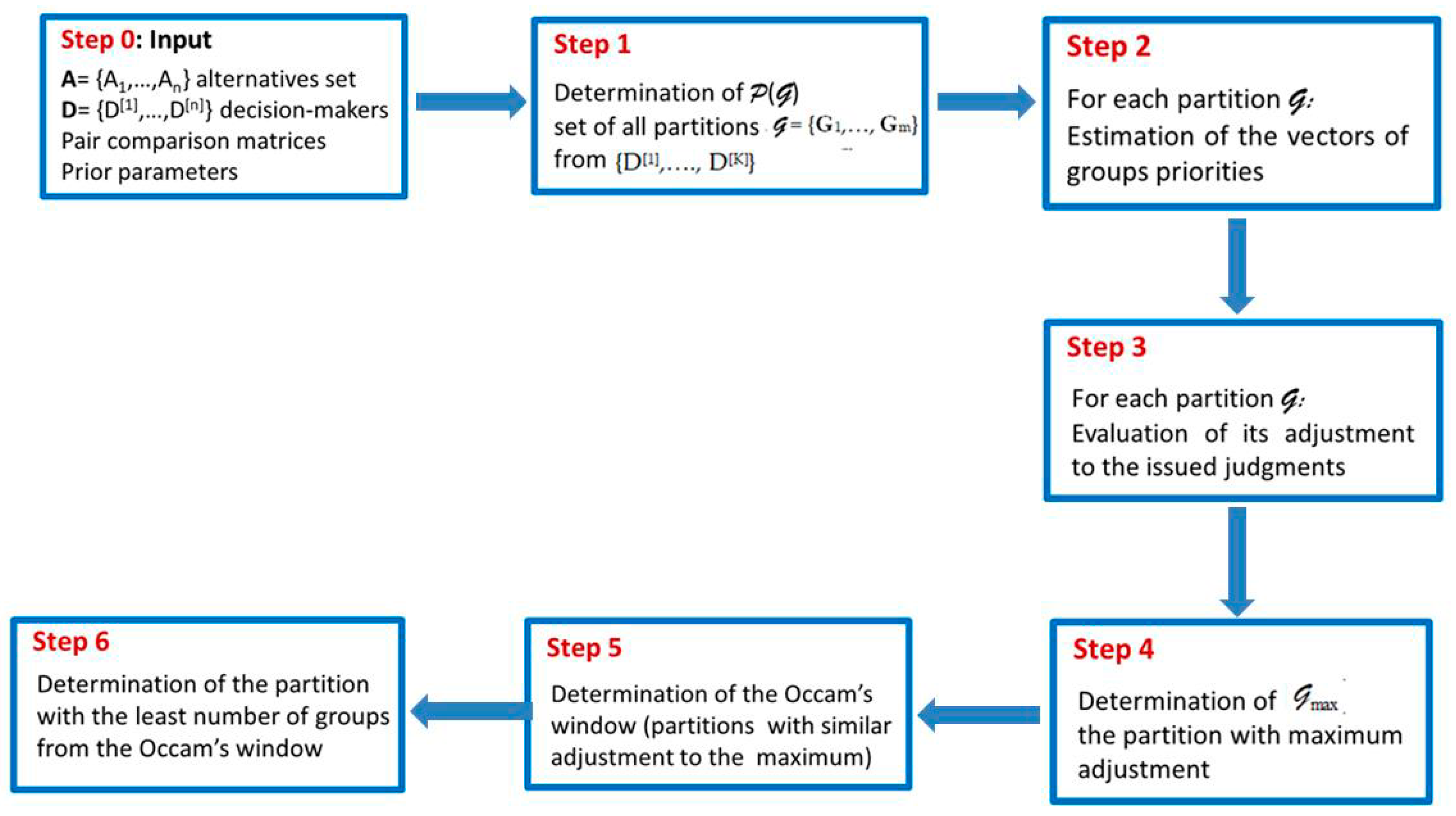
where $\left[Y|{\mathcal{G}}_{\max }\right]={\max }_{\mathcal{G}\in \mathrm{\wp }\left(D\right)}\left[Y|\mathcal{G}\right]$ and gives us the ‘Occam’s window’ of our problem [10]. The partitions could be taken as starting points for subsequent negotiation processes in order to reach an agreement among the decision makers that is as representative as possible. In our case, we look for the partitions of the window that have the least number of groups, since it can be foreseen that the fewer groups there will be, the easier it will be to reach more representative agreements because there are fewer disparate opinions. In order to do this, we use an exhaustive search algorithm that calculates the values of [Y|$\mathcal{G}$] for all the elements of ℘(D) using expression (19). Then $\mathcal{G}$_max is determined and, from this, the partitions of Occam’s window that verify (20) are identified. Other methods for consensus searching in group decision making can be seen in references [11,12,13,14,15,16].

Figure 1 shows the main steps for determining the groups with homogeneous opinions.

4. Case Study

In September 2006 the Government of Aragón and the Zaragoza City Council advanced the ‘Zaragoza Plan for Sustainable Mobility’, which led to the construction of the city’s Tram Line 1 that was completed in 2013. The construction was controversial and in the following municipal elections, the political parties presented their proposals for improving transport in the city. Representatives of the main political parties (PSOE, PP and CHA) attended the university to explain their preferred alternative. The case study concerns a citizen participation project in a local community which contemplated alternatives put forward by the political parties during the municipal elections for the extension of the city tram network.

Eleven students (K = 11) from the ‘Electronic-Government and Public Decisions’ course of the Faculty of Economics and Business at the University of Zaragoza (Spain) were involved in its implementation.

There were 4 alternatives:

A1

Build a new tram line

A2

Use a tram and bus combination called Tranbus

A3

Use a tram combination with commuter lines

A4

Do nothing

As the construction of Line 1 had a high economic cost, and the selection of any of first three alternatives assumes a significant investment, a fourth alternative (no cost) was included. The selection problem was solved using the Analytic Hierarchy Process [2]. The hierarchical model comprised four levels (the goal, 3 criteria, 9 attributes and 4 alternatives).

The results of the Investment Cost attribute have been used to illustrate the proposed methodology. The prior distribution parameters were c₀ = 0.1, n₀ = 1 and ${\mathrm{s}}_0^2$ = 0.0014 (corresponding to take ${\mathsf{\sigma }}_{\max }^2$ = 0.35 and α = 0.05) and β = 0.05. The number of partitions was equal to the 678,570 that were processed in 98.84 s of CPU by a Toshiba Ultrabook KIRA with Intel (R) Core™ i7-4510U CPU @ 2.00GHz 2.60 GHz (64 bits) and 8 Gb of RAM.

The resulting number of groups was equal to five and the most probable composition was: G₁ = {D₁, D₂, D₃, D₇}, G₂ = {D₄, D₁₀}, G₃ = {D₅, D₆}, G₄ = {D₉}, G₅ = {D₁₁}. The results obtained are shown in

Table 1. Priorities and consistency for each decision maker and each group.

Decision Maker	Priorities				Consistency
	w1	w2	w3	w4
D1	0.1285	0.2860	0.1275	0.4511	0.1412
D2	0.0899	0.2500	0.1418	0.5110	0.2042
D3	0.0900	0.4759	0.1582	0.2705	0.1363
D7	0.0587	0.2501	0.1839	0.5026	0.1405
G1	0.0879	0.3076	0.1518	0.4502	0.2790
D4	0.5748	0.1406	0.1086	0.1721	0.1214
D10	0.6318	0.1809	0.0797	0.1044	0.1046
G2	0.6139	0.1600	0.0926	0.1318	0.1602
D5	0.4021	0.1570	0.0758	0.3613	0.0888
D6	0.2131	0.1057	0.0542	0.6194	0.2849
D8	0.1388	0.2763	0.0578	0.5197	0.2186
G3	0.2321	0.1676	0.0617	0.5338	0.4071
D9	0.2846	0.0871	0.5503	0.0720	0.2186
G4	0.2846	0.0871	0.5503	0.0720	0.2186
D11	0.1228	0.4684	0.2736	0.1294	0.1261
G5	0.1228	0.4684	0.2736	0.1294	0.1261

in bold the highest priority.

,

Table 2. Alpha distributions for each decision maker and each group.

Decision Maker	Alternatives
	A1	A2	A3	A4
D1	0.30	6.11	0.00	93.59
D2	0.19	2.71	0.04	97.06
D3	0.00	96.75	0.00	3.25
D7	0.01	1.75	0.04	98.20
G1	0.00	2.69	0.00	97.31
D4	99.23	0.03	0.00	0.74
D10	99.92	0.02	0.00	0.06
G2	99.96	0.00	0.00	0.04
D5	63.16	0.01	0.00	36.83
D6	5.24	0.00	0.00	94.76
D8	1.09	3.92	0.00	94.99
G3	2.96	0.00	0.00	97.04
D9	5.49	0.00	94.51	0.00
G4	5.49	0.00	94.51	0.00
D11	0.01	98.75	1.20	0.04
G5	0.01	98.75	1.20	0.04

in bold the probabilities higher than 20%.

and

Table 3. Gamma distributions for each decision maker (D_i) and each group (G_j) (probabilities higher than 20% are in bold).

Decision Maker	Rankings
	1234 †	1243	1324	1342	1432	1423	2134	2143	2314	2341	2431	2413	3214	3241	3124	3142	3412	3421	4231	4213	4321	4312	4132	4123
D1	0.02	0.17	0.00	0.00	0.00	0.11	0.01	0.64	0.00	0.01	0.51	4.94	0.00	0.00	0.00	0.00	0.00	0.00	49.20	43.98	0.09	0.01	0.01	0.30
D2	0.05	0.10	0.00	0.00	0.00	0.04	0.01	0.23	0.00	0.00	0.87	1.60	0.00	0.00	0.00	0.00	0.01	0.03	86.05	8.68	2.10	0.05	0.03	0.15
D3	0.00	0.00	0.00	0.00	0.00	0.00	0.43	0.57	0.21	1.05	91.49	3.00	0.00	0.00	0.00	0.00	0.00	0.00	3.20	0.02	0.03	0.00	0.00	0.00
D7	0.01	0.00	0.00	0.00	0.00	0.00	0.00	0.05	0.02	0.04	1.55	0.09	0.00	0.00	0.01	0.00	0.00	0.03	89.78	0.07	8.33	0.00	0.01	0.01
G1	0.00	0.00	0.00	0.00	0.00	0.00	0.00	0.00	0.00	0.00	2.28	0.41	0.00	0.00	0.00	0.00	0.00	0.00	96.94	0.36	0.01	0.00	0.00	0.00
D4	1.75	20.98	0.23	0.40	8.64	67.23	0.00	0.01	0.00	0.00	0.00	0.02	0.00	0.00	0.00	0.00	0.00	0.00	0.00	0.01	0.01	0.02	0.41	0.29
D10	8.90	88.84	0.01	0.01	0.06	2.10	0.00	0.01	0.00	0.00	0.00	0.01	0.00	0.00	0.00	0.00	0.00	0.00	0.00	0.01	0.01	0.00	0.00	0.04
G2	2.46	80.42	0.00	0.02	0.15	16.91	0.00	0.00	0.00	0.00	0.00	0.00	0.00	0.00	0.00	0.00	0.00	0.00	0.00	0.00	0.00	0.00	0.01	0.03
D5	0.00	0.29	0.00	0.00	0.04	62.83	0.00	0.01	0.00	0.00	0.00	0.00	0.00	0.00	0.00	0.00	0.00	0.00	0.00	0.08	0.00	0.00	0.06	36.69
D6	0.01	0.15	0.00	0.00	0.09	4.99	0.00	0.00	0.00	0.00	0.00	0.00	0.00	0.00	0.00	0.00	0.00	0.00	0.36	3.63	0.16	0.16	1.99	88.46
D8	0.01	0.64	0.01	0.00	0.00	0.43	0.00	0.57	0.00	0.00	0.00	3.35	0.00	0.00	0.00	0.00	0.00	0.00	2.27	90.83	0.00	0.01	0.01	1.87
G3	0.00	0.03	0.00	0.00	0.00	2.93	0.00	0.00	0.00	0.00	0.00	0.00	0.00	0.00	0.00	0.00	0.00	0.00	0.00	11.32	0.00	0.00	0.00	85.72
D9	0.00	0.00	5.37	0.12	0.00	0.00	0.00	0.00	0.00	0.00	0.00	0.00	0.05	0.03	66.57	26.61	1.08	0.17	0.00	0.00	0.00	0.00	0.00	0.00
G4	0.00	0.00	5.37	0.12	0.00	0.00	0.00	0.00	0.00	0.00	0.00	0.00	0.05	0.03	66.57	26.61	1.08	0.17	0.00	0.00	0.00	0.00	0.00	0.00
D11	0.01	0.00	0.00	0.00	0.00	0.00	1.14	0.00	43.39	53.94	0.28	0.00	0.28	0.88	0.00	0.00	0.00	0.04	0.03	0.00	0.01	0.00	0.00	0.00
G5	0.01	0.00	0.00	0.00	0.00	0.00	1.14	0.00	43.39	53.94	0.28	0.00	0.28	0.88	0.00	0.00	0.00	0.04	0.03	0.00	0.01	0.00	0.00	0.00

^† 1234 denotes the ranking A₁ > A₂ > A₃ > A₄.

. More specifically, Table 1 contains the posterior medians of the priorities of each alternative for each decision maker and each group. Table 2 shows the posterior probabilities that each alternative would be the most preferred, corresponding to the Pα distributions. Table 3 gives the probabilities for each ranking corresponding to the Pγ distributions. The values were calculated from (7)–(8) and (11)–(12), as described in Section 2.2, using S = 10,000 simulations.

So, for example, group G1 made up of decision makers D₁, D₂, D₃ and D₇, gives the highest priority (0.4502) to alternative A₄, followed by the alternatives A₂ (priority 0.3076), A₃ (0.1518) and A₁ (0.0879) (see Table 1). This ranking is also reflected by its Pα and Pγ distributions, which give the maximum posterior probabilities to the A₄ alternative (97.31%, see Table 2) and the ranking 4231 (96.94%, see Table 3). Even though the individual opinion of D₃ is different to the rest of the members of the group (their preferred alternative is A₂ and the ranking is 2431), the consistency of the group G₁ (0.2790) is good, being lower than the maximum level of inconsistency 0.35. This is due to the high priority of D₃ for alternative A₄ (0.2705) and the similarity of their priorities to alternatives A₁ and A₃ which means that G1 can be considered as a homogeneous group.

From the tables, it can be observed that the compositions of the groups are very much determined by their similarity to the most preferred alternative. The decision makers from groups G₁ and G₃ mostly prefer the alternative A₄, those from group G₂ prefer alternative A₁, those from G₃ prefer alternative A₃ and those from G₄ prefer alternative A₂ (see Table 1 and Table 2). However, groups G₁ and G₃ differ in the rankings (see Table 3). The decision makers from the group G₁ tend to prefer the 4231 ranking, while those from the group G₃ prefer 4123. Nevertheless, preferences within each group are not completely homogeneous; in group G₁, decision-maker D₃ shows a greater preference for alternative A₂. This opinion is shared with decision maker D₁₁ of group G₄, although it assigns a priority 0.2705 to alternative A₄ that justifies its inclusion in group G₁. Something similar happens in group G_3, in which decision maker D₅ shows a greater preference for alternative A₁, although it assigns a non-negligible priority (0.3613) to alternative A₄ and to the ranking 4123, hence its inclusion in group G₃.

The consistency levels of the actors and most of the groups are acceptable (<0.35). The only exception is G₃ whose consistency is estimated as 0.4071, but with a 95% credibility interval [0.20, 1.43] that does not reject the consistency hypothesis ${\mathsf{\sigma }}^{2\left({\mathrm{G}}_3\right)}\le 0.35$.

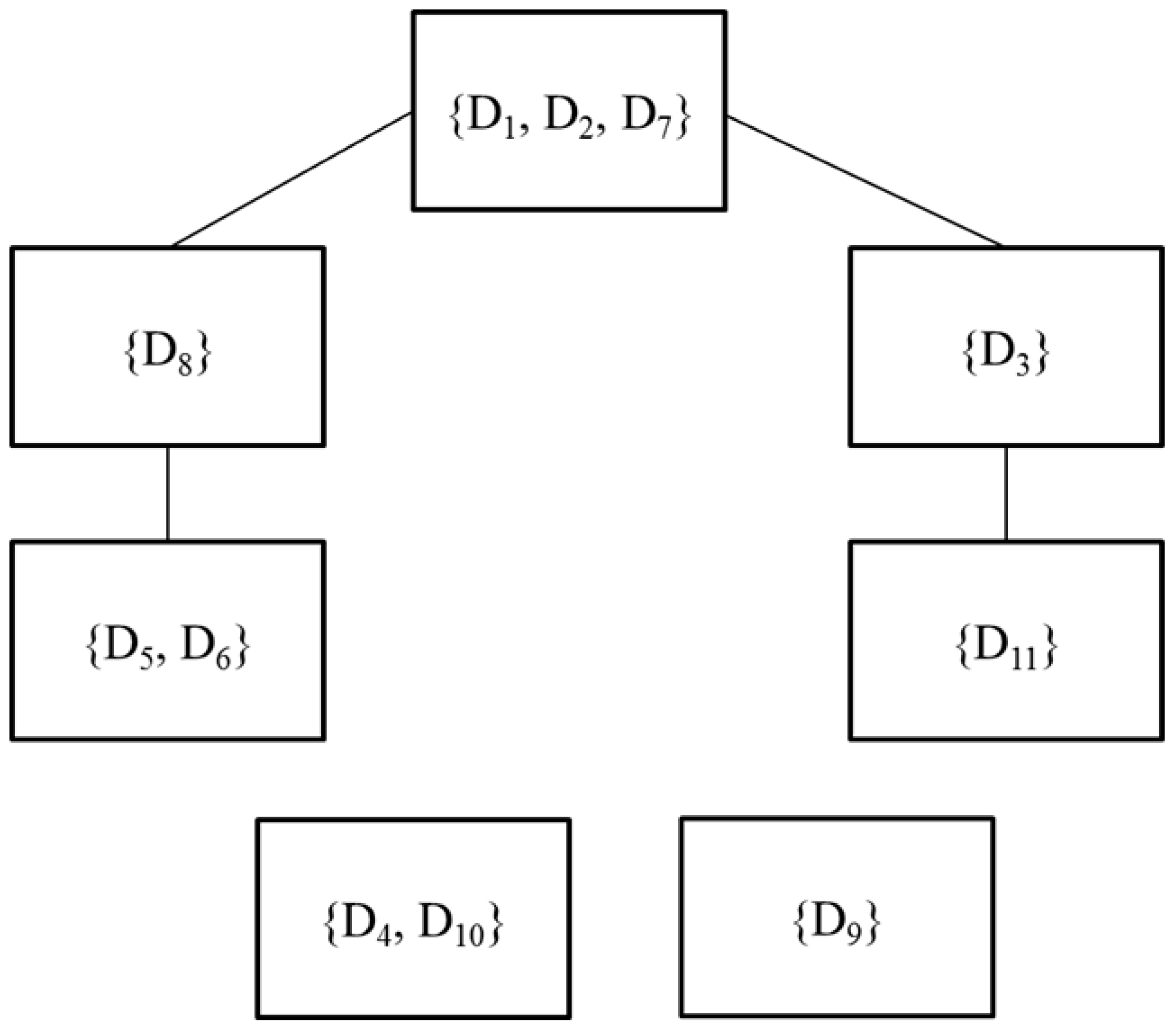
The ambiguities of the opinions are revealed if we analyse the partitions selected by Occam’s window with the smaller number of groups, included in

Table 4. Partitions selected by the Occam window.

Partition	D1	D2	D3	D4	D5	D6	D7	D8	D9	D10	D11	Ratio †
1	1	1	1	2	3	3	1	3	4	2	5	1.00
2	1	1	2	3	4	4	1	4	5	3	2	0.48
3	1	1	1	2	3	3	1	1	4	2	5	0.42
4	1	1	2	3	4	4	1	1	5	3	2	0.15

^† The ratio calculates the quotient of the posterior probability for the most probable model and that for the model corresponding to each partition.

and Figure 2. Figure 2 incorporates, in each node, the groups of decision makers that are classified together in all the selected partitions and includes a link between two nodes if their components are classified together in some of the partitions. Most of the decision makers are linked because of their preferences for alternatives A₂ and A₄, the latter being the alternative which most decision makers support. Only D₄, D₉ and D₁₀ are isolated because of their preferences for alternatives A₁ (D₄ and D₁₀) and A₃ (D₉).

There are 4 homogeneous groups: {D₁, D₂, D₇} that prefer alternative A₄ and the ranking 4231; {D₅, D₆} position alternatives A₂ and A₃ in the last places and they show a non-negligible preference for A₄; {D₄, D₁₀} prefer alternative A₁ and put A₃ in last place; decision maker {D₉} prefers A₃. Decision makers D₃, D₈, D₁₁ are in more intermediate and ambiguous positions. In the case of D₃, this is due to the greater preference for A₂ (shared with D₁₁) and the non-negligible preference for A₄ (which places them close to the group {D₁, D₂, D₇}). In the case of D₈, the intermediate position is due to their preferences for A₄ and A₂, in that order, which places them close to the group {D₁, D₂, D₇}, as well as to the rejection of A₃, which places them close to the group {D₅, D₆}.

In order to achieve as broad an agreement as possible, alternative A₄ could be suggested, given that a majority of decision makers (in groups G₁ and G₃) showed a preference for it. The negotiation should be aimed at convincing decision makers D₄, D₉, D₁₀ and D₁₁.

With regards to the practical implications of the Bayesian procedure proposed in this work, it is worth mentioning that, as in AHP, these applications are numerous, especially in matters of strategic planning where the number of actors is not usually very high.

5. Conclusions

This paper has proposed a methodology for the identification of homogenous opinion groups with AHP in a local context. The methodology is based on the use of Bayesian processes for the selection of hierarchical models that describe the judgments issued by each decision maker in their matrices of pairwise comparisons based on a set of priorities common to each of the members of the group.

Using an exhaustive search method of the most compatible partitions with the judgments issued, the Occam’s window of the compared models is defined. From these models it has been shown how it is possible to describe the existing opinions in the groups, information that can be very useful to identify consensus paths among the decision makers that can culminate in a more representative decision-making process.

The search method works in a local AHP context, but has some limitations. First, it functions if the number of decision makers is not very high (≤11). The total number of partitions of the set of decision makers is equal to the Bell number ${\mathrm{B}}_{\mathrm{K}}={\displaystyle \sum _{\mathrm{k}=0}^{\mathrm{K}-1}\left(\begin{array}{c}\mathrm{K}-1\\ \mathrm{k}\end{array}\right){\mathrm{B}}_{\mathrm{k}}}$ with B₀ = 1, B₁ = 1. The larger the number of decision makers, the more computationally infeasible is the problem. In our case (K = 11), the number of possible partitions is 687,570, which is computationally feasible. For instance, if K = 22 the number is 4507 × 10¹⁵, then it is necessary to use algorithms that approximately determine Occam’s window.

We are currently experimenting with stochastic search algorithms and the results obtained will be published in a future work. A second limitation is that it is necessary that the groups constitute a partition of the set of decision makers and this implies that a decision maker cannot belong to more than one group. Even though this requirement decreases the computational time of the algorithm, it also reduces the flexibility of the method. The development of search strategies that eliminate this unrealistic assumption is worthy of consideration. Finally, it would be interesting to extend the methodology to a global context in which a hierarchy of criteria and sub-criteria is used.

References

- Moreno-Jiménez, J.M.; Vargas, L.G. Cognitive Multicriteria Decision Making and the Legacy of AHP. Estud. Econ. Apl. 2018, 36, 67–80. [Google Scholar]
- Saaty, T.L. The Analytic Hierarchy Process; Mc Graw-Hill: New York, NY, USA, 1980. [Google Scholar]
- Saaty, T.L. Group decision making and the AHP. In The Analytic Hierarchy Process; Golden, B.L., Wasil, E.A., Harker, P.T., Eds.; Springer: Berlin/Heidelberg, Germany, 1989; pp. 59–67. [Google Scholar]
- Ramanathan, R.; Ganesh, L.S. Group preference aggregation methods employed in AHP: An evaluation and intrinsic process for deriving members’ weightages. Eur. J. Oper. Res. 1994, 79, 249–265. [Google Scholar] [CrossRef]
- Forman, E.; Peniwati, K. Aggregating individual judgements and priorities with the analytic hierarchy process. Eur. J. Oper. Res. 1998, 108, 165–169. [Google Scholar] [CrossRef]
- Altuzarra, A.; Moreno-Jiménez, J.M.; Salvador, M. A Bayesian priorization procedure for AHP-group decision making. Eur. J. Oper. Res. 2007, 182, 367–382. [Google Scholar] [CrossRef]
- Gelman, A.; Carlin, J.; Stern, H.; Dunson, D.; Vehtary, A.; Rubin, D. Bayesian Data Analysis, 3rd ed.; CRC Press: Boca Raton, FL, USA, 2014. [Google Scholar]
- Aguarón, J.; Moreno-Jiménez, J.M. The geometric consistency index: Approximate thresholds. Eur. J. Oper. Res. 2003, 147, 137–145. [Google Scholar] [CrossRef]
- Kass, R.E.; Raftery, A.E. Bayes factors. J. Am. Stat. Assoc. 1995, 90, 773–795. [Google Scholar] [CrossRef]
- Madigan, D.; Raftery, A.E. Model Selection and Accounting for Model Uncertainty in Graphical Models Using Occam’s Window. J. Am. Stat. Assoc. 1994, 89, 1535–1546. [Google Scholar] [CrossRef]
- Altuzarra, A.; Moreno-Jiménez, J.M.; Salvador, M. A Consensus building in AHP-group decision making: A Bayesian approach. Oper. Res. 2010, 58, 1755–1773. [Google Scholar] [CrossRef]
- Chen, S.M.; Lin, T.E.; Lee, L.W. Group Decision Making using incomplete fuzzy preference relations based on the additive consistency and the order consistency. Inf. Sci. 2014, 259, 1–15. [Google Scholar] [CrossRef]
- Herrera-Viedma, E.; Cabrerizo, F.J.; Kacprzyk, J.; Pedrycz, W. A review of soft consensus models in a fuzzy environment. Inf. Fusion 2014, 17, 4–13. [Google Scholar] [CrossRef]
- Wang, Z.J.; Lin, J. Ratio-based similarity analysis and consensus building for group decision making with interval reciprocal preference relations. Appl. Soft Comput. 2016, 42, 260–275. [Google Scholar] [CrossRef]
- Dong, Y.C.; Ding, Z.G.; Martínez, L.; Herrera, F. Managing consensus based on leadership in opinion dynamics. Inf. Sci. 2017, 397, 187–205. [Google Scholar] [CrossRef]
- Wu, Z.B.; Xu, J. A consensus model for large-scale group decision making with hesitant fuzzy information and changeable clusters. Inf. Fusion 2018, 41, 217–231. [Google Scholar] [CrossRef]
Figure 1.
Steps of the proposed methodology.
Figure 2.
Relations of opinions existing in D.