Improving the Computational Efficiency of a Variant of Steffensen’s Method for Nonlinear Equations

Abstract

Steffensen-type methods with memory were originally designed to solve nonlinear equations without the use of additional functional evaluations per computing step. In this paper, a variant of Steffensen’s method is proposed which is derivative-free and with memory. In fact, using an acceleration technique via interpolation polynomials of appropriate degrees, the computational efficiency index of this scheme is improved. It is discussed that the new scheme is quite fast and has a high efficiency index. Finally, numerical investigations are brought forward to uphold the theoretical discussions.

1. Introduction

One of the commonly encountered topics in computational mathematics is to tackle solving a nonlinear algebraic equation. The equation can be presented as in the scalar case $f\left(x\right)=0$, or more complicated as a system of nonlinear algebraic equations. The procedure of finding the solutions (if it exists) cannot be done analytically. In some cases, the analytic techniques only give the real result while its complex zeros should be found and reported. As such, numerical techniques are a viable choice for solving such nonlinear problems. Each of the existing computational procedures has their own domain of validity with some pros and cons [1,2].

Two classes of methods with the use of derivatives and without the use of derivatives are known to be useful depending on the application dealing with [3]. In the derivative-involved methods, a larger attraction basin along with a simple coding effort for higher dimensional problems is at hand which, in derivative-free methods, the area of choosing the initial approximations is smaller and extending to higher dimensional problems is via the application of a divided difference operator matrix, which is basically a dense matrix. However, the ease in not computing the derivative and, subsequently, the Jacobians, make the application of derivative-free methods more practical in several problems [4,5,6,7].

Here, an attempt is made at developing a computational method which is not only efficient in terms of the computational efficiency index, but also in terms of larger domains for the choice of the initial guesses/approximations for starting the proposed numerical method.

The Steffensen’s method [8] for solving nonlinear scalar equations has quadratic convergence for simple zeros and given by:

$$\{\begin{array}{c}{x}_{k+1}=x_k-\frac{f\left(x_k\right)}{\begin{array}{c}f\\ \left[x_k,w_k\right]\end{array}},\\ w_k=x_k+\beta f\left(x_k\right),\beta \in R\backslash \left\{0\right\},k\ge 0,\end{array}$$

(1)

where the two-point divided difference is defined by:

$$f\left[x_k,w_k\right]=\frac{f\left(x_k\right)-f\left(w_x\right)}{x_k-w_k},$$

This scheme needs two function evaluations per cycle. Scheme (1) shows an excellent tool for constructing efficient iterative methods for nonlinear equations. This is because it is derivative-free with a free parameter. This parameter can, first of all, enlarge the attraction basins of Equation (1) or any of its subsequent methods and, second, can directly affect the improvement of the R-order of convergence and the efficiency index.

Recalling that Kung and Traub conjectured that the iterative method without memory based on m functions evaluation per iteration attain the optimal convergence of order $2^{m-1}$ [9,10].

The term “with memory” means that the values of the function associated with the computed approximations of the roots are used in subsequent iterations. This is unlike the term “without memory” in which the method only uses the current values to find the next estimate. As such, in a method with memory, the calculated results up to the desired numbers of iterations should be stored and then called to proceed.

Before proceeding the given idea to improve the speed of convergence, efficiency index, and the attraction basins, we provide a short literature by reviewing some of the existing methods with accelerated convergence order. Traub [11] proposed the following two-point method with memory of order 2.414:

$$\{\begin{array}{c}{x}_{k+1}=x_k-\frac{f\left(x_k\right)}{f\left[x_k,x_k+{\beta }_{k}f(x_k\right)]},\\ {\beta }_k=\frac{-1}{f\left[x_k,z_{k-1}\right]},\end{array}$$

(2)

where $z_{k-1}=x_{k-1}+{\beta }_{k-1}f\left(x_{k-1}\right)$, and ${\beta }_0=-\mathrm{sign}\left(f^{\prime }\left(x_0\right)\right)$ or $-\frac{1}{f\left[x_0,x_0+f\left(x_0\right)\right]}$. This is one of the pioneering and fundamental methods with memory for solving nonlinear equations.

Džunić in [12] suggested an effective bi-parametric iterative method with memory of $\frac{1}{2}\left(3+\sqrt{17}\right)$ R-order of convergence as follows:

$$\{\begin{array}{c}{w}_k=x_k+{\beta }_{k}f\left(x_k\right),\\ {\beta }_k=-\frac{1}{N_2^{\prime }\left(x_k\right)},{\zeta }_k=-\frac{N_3^{″}\left(w_k\right)}{2N_3^{\prime }\left(w_k\right)},k\ge 1,\\ x_{k+1}=x_k-\frac{f\left(x_k\right)}{f\left[x_k,w_k\right]+{\zeta }_{k}f\left(w_k\right)}k\ge 0.\end{array}$$

(3)

Moreover, Džunić and Petković [13] derived the following cubically convergent Steffensen-like method with memory:

$$\{\begin{array}{c}{x}_{k+1}=x_k-\frac{f\left(x_k\right)}{f\left[x_k,x_k+{\beta }_{k}f(x_k\right)]},\\ {\beta }_k=\frac{-1}{f\left[x_k,z_{k-1}\left]+f\right[x_k,x_{k-1}\left]+f\right[x_{k-1},z_{k-1}\right]},\end{array}$$

(4)

where $z_{k-1}=x_{k-1}+{\beta }_{k-1}f\left(x_{k-1}\right)$ depending on the second-order Newton interpolation polynomial.

Various Steffensen-type methods are proposed in [14,15,16,17].

In fact, it is possible to improve the performance of the aforementioned method by considering several more sub-steps and improve the computational efficiency index via multi-step iterative methods. However, this procedure is more computational burdensome. Thus, the motivation here is to know that is it possible to improve the performance of numerical methods in terms of the computational efficiency index, basins of attraction, and the rate of convergence without adding more sub-steps and propose a numerical method as a one-step solver.

Hence, the aim of this paper is to design a one-step method with memory which is quite fast and has an improved efficiency index, based on the modification of the one-step method of Steffensen (Equation (1)) and increase the convergence order to 3.90057 without any additional functional evaluations.

The rest of this paper is ordered as follows: In Section 2, we develop the one-point Steffensen-type iterative scheme (Equation (1)) with memory which was proposed by [18]. We present the main goal in Section 3 by approximating the acceleration parameters involved in our contributed scheme by Newton’s interpolating polynomial and, thus, improve the convergence R-order. The numerical reports are suggested in Section 4 to confirm the theoretical results. Some discussions are given in Section 5.

2. An Iterative Method

The following iterative method without memory was proposed by [18]:

$$\{\begin{array}{c}{w}_k=x_k-\beta f\left(x_k\right),\\ x_{k+1}=x_k-\frac{f\left(x_k\right)}{f\left[x_k,w_k\right]}\left(1+\zeta \frac{f\left(w_k\right)}{f\left[x_k,w_k\right]}\right),\zeta \in \mathbb{R},\end{array}$$

(5)

with the following error equation to improve the performance of (1) in terms of having more free parameters:

$$e_{k+1}=-\left(-1+\beta f^{\prime }\left(\alpha \right)\right)\left(c_2-\zeta \right)e_k^2+O\left(e_k^3\right),$$

(6)

where $c_i=\frac{1}{i!}\frac{f^{\left(i\right)}\left(\alpha \right)}{f^{\prime }\left(\alpha \right)}$. Using the error Equation (6), to derive Steffensen-type iterative methods with memory, we calculate the following parameters: $\beta ={\beta }_k$, $\zeta ={\zeta }_k,$ by the formula:

$$\{\begin{array}{c}{\beta }_k=\frac{1}{\overline{f^{\prime }}\left(x_{\alpha }\right)},\\ {\zeta }_k={\overline{c}}_2,\end{array}$$

(7)

for $k=1,2,3,\cdots$, while $\overline{f^{\prime }}\left(x_{\alpha }\right)$, ${\overline{c}}_2$ are approximations to $f\left(\alpha \right)$ and $c_2$, respectively; where $\alpha$ is a simple zero of $f\left(x\right)$. In fact, Equation (7) shows a way to minimize the asymptotic error constant of Equation (6) by making this coefficient closer and closer to zero when the iterative method is converging to the true solution.

The initial estimates ${\beta }_0$ and ${\zeta }_0$ must be chosen before starting the process of iterations. We state the Newton’s interpolating polynomial of fourth and fifth-degree passing through the saved points as follows:

$$\{\begin{array}{c}{N}_4\left(t\right)=N_4\left(t;x_k,w_{k-1},x_{k-1},w_{k-2},x_{k-2}\right),\\ N_5\left(t\right)=N_5\left(t;w_k,x_k,w_{k-1},x_{k-1},w_{k-2},x_{k-2}\right).\end{array}$$

(8)

Recalling that $N\left(t\right)$ is an interpolation polynomial for a given set of data points also known as the Newton’s divided differences interpolation polynomial because the coefficients of the polynomial are calculated using Newton’s divided differences method. For instance, here the set of data points for $N_4\left(t\right)$ are $\{\left\{x_k,f\left(x_k\right)\right\},\left\{w_{k-1},f\left(w_{k-1}\right)\right\},\left\{x_{k-1},f\left(x_{k-1}\right)\right\},\left\{w_{k-2},f\left(w_{k-2}\right)\right\}$ $,\left\{x_{k-2},f\left(x_{k-2}\right)\right\}\}$.

Now, using some modification on Equation (5) we present the following scheme:

$$\{\begin{array}{c}{w}_k=x_k-{\beta }_{k}f\left(x_k\right),\\ {\beta }_k=\frac{1}{N_4^{\prime }\left(x_k\right)},{\zeta }_k=\frac{N_5^{″}\left(w_k\right)}{2N_5^{\prime }\left(w_k\right)},k\ge 2,\\ x_{k+1}=x_k-\frac{f\left(x_k\right)}{f\left[x_k,w_k\right]}\left(1+{\zeta }_k\frac{f\left(w_k\right)}{f\left[x_k,w_k\right]}\right),k\ge 0.\end{array}$$

(9)

Noting that the accelerator parameters ${\beta }_k,{\zeta }_k$ are getting updated and then used in the iterative method right after the second iterations, viz, $k\ge 2$. This means that the third line of Equation (9) is imposed at the beginning and after that the computed values are stored and used in the subsequent iterates. For $k=1$, the degree of Newton interpolation polynomials would be two and three. However, for $k\ge 2$, interpolations of degrees four and five as given in Equation (8) can be used to increase the convergence order.

Additionally speaking, this acceleration of convergence would be attained without the use any more functional evaluations as well as imposing more steps. Thus, the proposed scheme with memory (Equation (9)) can be attractive for solving nonlinear equations.

3. Convergence Analysis

In this section, we show the convergence criteria of Equation (9) using Taylor’s series expansion and several extensive symbolic computations.

Theorem 1.

Let the function$f\left(x\right)$be sufficiently differentiable in a neighborhood of its simple zero$\alpha$. If an initial approximation$x_0$is necessarily close to$\alpha$. Then, R-order of convergence for the one-step method (Equation (9)) with memory is 3.90057.

Proof. 

The proof is done using the definition of the error equation as the difference between the k-estimate and the exact zero along with symbolic computations. Let the sequence $\left\{x_k\right\}$ and $\left\{w_k\right\}$ have convergence orders $r$ and $p$, respectively. Namely,

$$\begin{array}{l}{e}_{k+1}~e_k^r,\hfill \end{array}$$

(10)

and:

$$\begin{array}{l}{e}_{w,k}~e_k^p,\hfill \end{array}$$

(11)

Therefore, using Equations (10) and (11), we have:

$$\begin{array}{l}{e}_{k+1}~e_k^r~e_{k-1}^{r^2}~e_{k-2}^{r^3},\hfill \end{array}$$

(12)

and:

$$\begin{array}{l}{e}_{w,k}~e_k^p~{(e_{k-1}^r)}^p~e_{k-2}^{p{r}^2}.\hfill \end{array}$$

(13)

The associated error equations to the accelerating parameters ${\beta }_k$ and ${\zeta }_k$ for Equation (9) can now be written as follows:

$$\begin{array}{l}{e}_{w,k}~\left(-1+{\beta }_k{f}^{\prime }\left(\alpha \right)\right)e_k\hfill \end{array},$$

(14)

and:

$$\begin{array}{l}{e}_{k+1}~-\left(-1+{\beta }_k{f}^{\prime }\left(\alpha \right)\right)\left(c_2-{\zeta }_k\right)e_k^2.\hfill \end{array}$$

(15)

On the other hand, by using a symbolic language and extensive computations one can find the following error terms for the involved terms existing in the fundamental error Equation (6):

$$\begin{array}{l}-1+{\beta }_k{f}^{\prime }\left(\alpha \right)~c_5{e}_{k-2}{e}_{k-1}{e}_{w,k-1}{e}_{w,k-2},\hfill \end{array}$$

(16)

$$c_2-{\zeta }_k~c_6{e}_{k-2}{e}_{k-1}{e}_{w,k-1}{e}_{w,k-2}$$

(17)

Combining Equations (14)–(17), we get that:

$$\begin{array}{l}{e}_{w,k}~e_{k-2}^{r^2+pr+r+p+1},\hfill \end{array}$$

(18)

$$\begin{array}{l}{e}_{k+1}~e_{k-2}^{2\left(r^2+pr+r+p+1\right)}.\hfill \end{array}$$

(19)

We now compare the left and right hand side of Equations (12)–(19) and Equations (13)–(18), respectively. Thus, we have the following nonlinear system of equations in order to find the final R-orders:

$$\{\begin{array}{c}{r}^{2}p-\left(r^2+pr+r+p+1\right)=0,\\ r^3-2\left(r^2+pr+r+p+1\right)=0.\end{array}$$

(20)

The positive real solution of (20) is $r=3.90057$ and $p=1.9502$. Therefore, the convergence R-order for Equation (9) is 3.90057. □

Since improving the convergence R-order is useless if the whole computational method is expensive, basically researcher judge on a new scheme based upon its computational efficiency index which is a tool in order to provide a trade-off between the whole computational cost and the attained R-order. Assuming the cost of calculating each functional evaluation is one, we can use the definition of efficiency index as $EI=p^{1/\theta }$, $\theta$ is the whole computational cost [19].

The computational efficiency index of Equation (9) is ${3.90057}^{\frac{1}{2}}\approx 1.97499\approx 2$, which is clearly higher than efficiency index $2^{\frac{1}{2}}\approx 1.4142$ of Newton’s and Steffensen’s methods, $3.56155{}^{\frac{1}{2}}$ $\approx 1.8872$ of (3) $3^{1/2}\approx 1.73205$ of Equation (4).

However, this improved computational efficiency is reported by ignoring the number of multiplication and division per computing cycle. By imposing a slight weight for such calculations one may once again obtain the improved computational efficiency of (9) in contrast to the existing schemes of the same type.

4. Numerical Computations

In this section, we compare the convergence performance of Equation (9), with three well-known iterative methods for solving four test problems numerically carried out in Mathematica 11.1. [20].

We denote Equations (1), (3), (5) and (9) with SM, DZ, PM, M4, respectively. We compare the our method with different methods, using ${\beta }_0=0.1$ and ${\zeta }_0=0.1$. Here, the computational order of convergence (coc) has been computed by the following formula [21]:

$$\begin{array}{l}coc=\frac{\ln |(f\left(x_k\right)/f\left(x_{k-1}\right)|}{\ln |(f\left(x_{k-1}\right)/f\left(x_{k-2}\right)|}\hfill \end{array}$$

(21)

Recalling that using a complex initial approximation, one is able to find the complex roots of the nonlinear equations using (9).

Experiment 1.

Let us consider the following nonlinear test function:

$$\begin{array}{l}{f}_1\left(x\right)=\left(x-2\tan \left(x\right)\right)\left(x^3-8\right),\hfill \end{array}$$

(22)

where$\alpha =2$and$x_0=1.7$.

Experiment 2.

We take into account the following nonlinear test function:

$$\begin{array}{l}{f}_2\left(x\right)=\left(x-1\right)\left(x^{10}+x^3+1\right)\sin \left(x\right),\hfill \end{array}$$

(23)

where$\alpha =1$and$x_0=0.7$.

Experiment 3.

We consider the following test problem now:

$$\begin{array}{l}{f}_3\left(x\right)=\frac{-x^3}{2}+2{\tan }^{-1}\left(x\right)+1,\hfill \end{array}$$

(24)

where$\alpha \approx 1.8467200$and$x_0=4$.

Experiment 4.

The last test problem is taken into consideration as follows:

$$f_4\left(x\right)={\tan }^{-1}\left(\exp \left(x+2\right)+1\right)+\tanh \left(\exp \left(-x\cos \left(x\right)\right)\right)-\sin \left(\pi x\right),$$

(25)

where$\alpha \approx -3.6323572···$and$x_0=-4.1$.

Table 1. Result of comparisons for the function $f_1$.

Methods	$\left|{\mathit{f}}_1\left({\mathit{x}}_3\right)\right|$	$\left|{\mathit{f}}_1\left({\mathit{x}}_4\right)\right|$	$\left|{\mathit{f}}_1\left({\mathit{x}}_5\right)\right|$	$\left|{\mathit{f}}_1\left({\mathit{x}}_6\right)\right|$	coc
SM	$4.1583$	$3.0743$	$1.4436$	$0.25430$	$2.00$
DZ	$0.13132$	$2.0026\times {10}^{-7}$	$1.0181\times {10}^{-27}$	$7.1731\times {10}^{-99}$	$3.57$
PM	$1.8921\times {10}^{-6}$	$4.5864\times {10}^{-24}$	$1.0569\times {10}^{-88}$	$7.5269\times {10}^{-318}$	$3.55$
M4	$9.1741\times {10}^{-6}$	$3.3242\times {10}^{-26}$	$4.4181\times {10}^{-103}$	$1.1147\times {10}^{-404}$	$3.92$

,

Table 2. Result of comparisons for the function $f_2$.

Methods	$\left|{\mathit{f}}_2\left({\mathit{x}}_5\right)\right|$	$\left|{\mathit{f}}_2\left({\mathit{x}}_6\right)\right|$	$\left|{\mathit{f}}_2\left({\mathit{x}}_7\right)\right|$	$\left|{\mathit{f}}_2\left({\mathit{x}}_8\right)\right|$	coc
SM	$-$	$-$	$-$	$-$	$-$
DZ	$0.14774$	$0.0016019$.	$1.3204\times {10}^{-10}$	$1.5335\times {10}^{-35}$	$3.56$
PM	$2.1191\times {10}^{-10}$	$8.0792\times {10}^{-35}$	$1.9037\times {10}^{-121}$	$3.7062\times {10}^{-430}$	$3.56$
M4	$5.9738\times {10}^{-15}$	$4.1615\times {10}^{-57}$	$1.7309\times {10}^{-220}$	$1.8231\times {10}^{-857}$	$3.90$

,

Table 3. Result of comparisons for the function $f_3$.

Methods	$\left|{\mathit{f}}_3\left({\mathit{x}}_3\right)\right|$	$\left|{\mathit{f}}_3\left({\mathit{x}}_4\right)\right|$	$\left|{\mathit{f}}_3\left({\mathit{x}}_5\right)\right|$	$\left|{\mathit{f}}_3\left({\mathit{x}}_6\right)\right|$	coc
SM	$0.042162$	$0.00012627$	$1.1589\times {10}^{-9}$	$9.7638\times {10}^{-20}$	$2.00$
DZ	$1.0219\times {10}^{-11}$	$4.4086\times {10}^{-44}$	$1.6412\times {10}^{-157}$	$1.5347\times {10}^{-562}$	$3.57$
PM	$7.9792\times {10}^{-8}$	$3.712\times {10}^{-30}$	$4.9556\times {10}^{-108}$	$2.9954\times {10}^{-386}$	$3.57$
M4	$4.4718\times {10}^{-6}$	$2.9187\times {10}^{-25}$	$4.7057\times {10}^{-101}$	$1.0495\times {10}^{-395}$	$3.89$

and

Table 4. Result of comparisons for the function $f_4$.

Methods	$\left|{\mathit{f}}_4\left({\mathit{x}}_3\right)\right|$	$\left|{\mathit{f}}_4\left({\mathit{x}}_4\right)\right|$	$\left|{\mathit{f}}_4\left({\mathit{x}}_5\right)\right|$	$\left|{\mathit{f}}_4\left({\mathit{x}}_6\right)\right|$	coc
SM	$0.00001166$	$3.7123\times {10}^{-10}$	$3.7616\times {10}^{-19}$	$3.8622\times {10}^{-37}$	$2.00$
DZ	$1.6\times {10}^{-13}$	$6.9981\times {10}^{-47}$	$1.0583\times {10}^{-164}$	$7.0664\times {10}^{-585}$	$3.57$
PM	$3.0531\times {10}^{-11}$	$3.2196\times {10}^{-38}$	$3.7357\times {10}^{-134}$	$6.5771\times {10}^{-476}$	$3.56$
M4	$2.5268\times {10}^{-13}$	$1.5972\times {10}^{-49}$	$2.8738\times {10}^{-191}$	$1.6018\times {10}^{-744}$	$3.90$

show that the proposed Equation (9) is of order 3.90057 and it is obviously believed to be of more advantageous than the other methods listed due to its fast speed and better accuracy.

For better comparisons, we present absolute residual errors $\left|f_{}\left(x\right)\right|$, for each test function which are displayed in Table 1, Table 2, Table 3 and Table 4. Additionally, we compute the computational order of convergence. Noting that we have used multiple precision arithmetic considering 2000 significant digits to observe and the asymptotic error constant and the coc as obviously as possible.

The results obtained by our proposed Equation (M4) are efficient and show better performance than other existing methods.

A significant challenge of executing high-order nonlinear solvers is in finding initial approximation to start the iterations when high accuracy calculating is needed.

To discuss further, mostly based on interval mathematics, one can find a close enough guess to start the process. There are some other ways to determine the real initial approximation to start the process. An idea of finding such initial guesses given in [22] is based on the useful commands in Mathematica 11.1 NDSolve [] for the nonlinear function on the interval $D=\left[a,b\right]$.

Following this the following piece of Mathematica code could give a list of initial approximations in the working interval for Experiment 4:

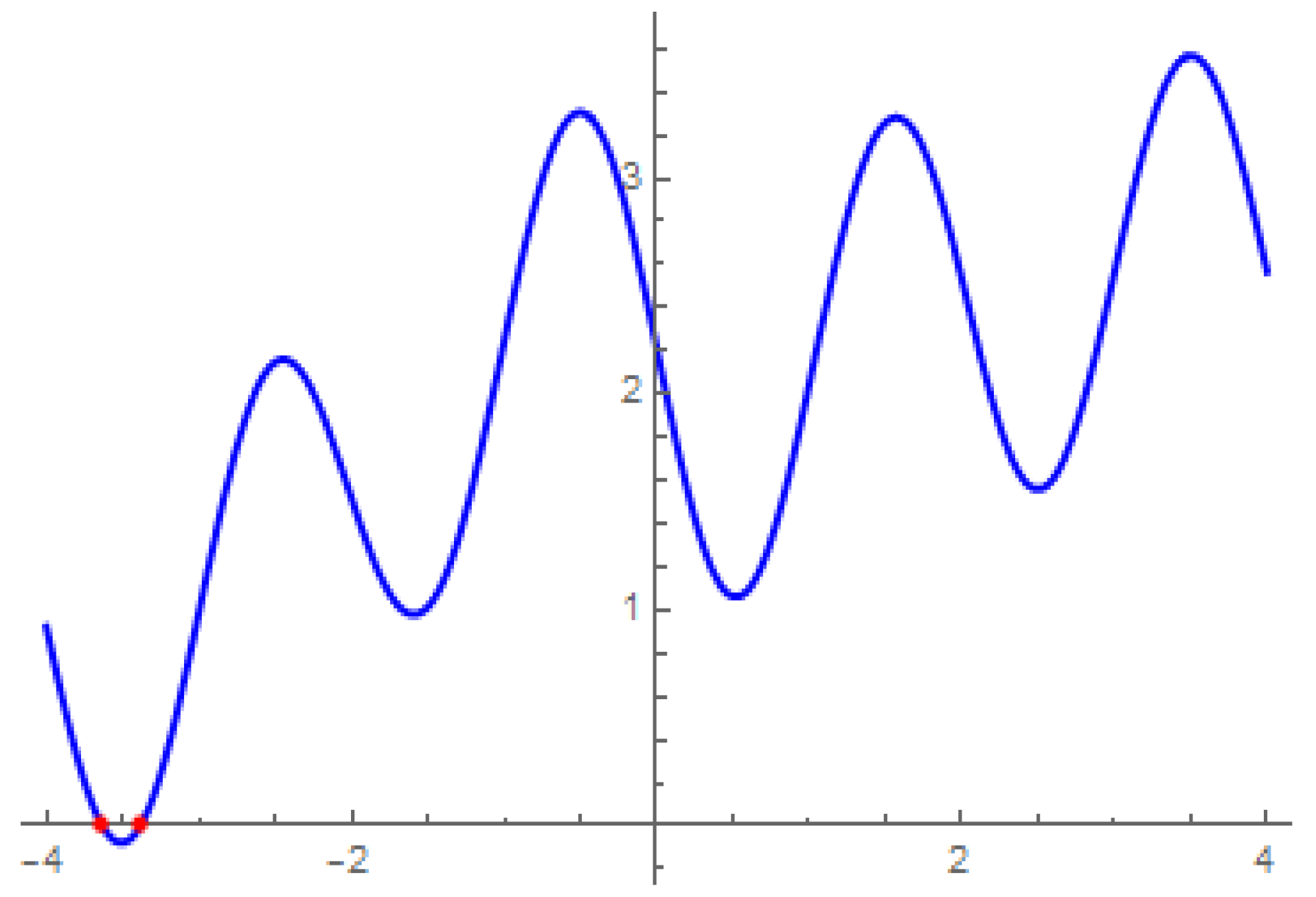
To check the position of the zero and the graph of the function, we can use the following code to obtain Figure 1.

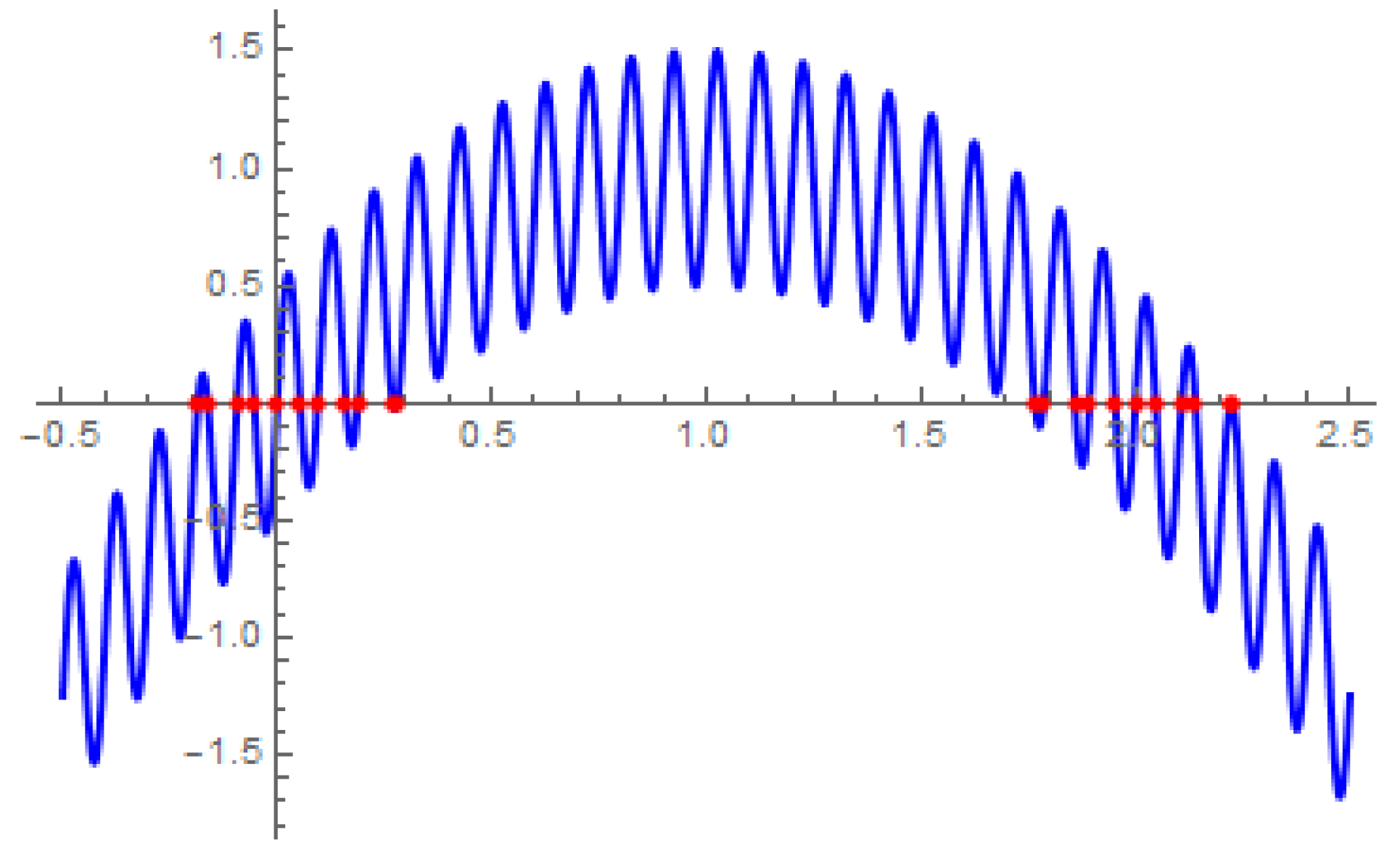
As a harder test problem, for the nonlinear function $g\left(x\right)=2x+0.5\sin \left(20\pi x\right)-x^2$, we can simply find a list of estimates as initial guesses using the above piece of codes as follows: $\left\{-0.185014,-0.162392,-0.0935912,-0.0535277,6.73675\times {10}^{-9},0.0533287,0.0941576,0.160021,0.188066,0.269075,0.279428,1.76552,1.78616,1.8588,1.89339,1.95294,2.,2.04692,2.10748,2.13979,2.2228,2.22471\right\}$. The plot of the function in this case is brought forward in Figure 2.

We observe that the two self-accelerating parameters ${\beta }_0$ and ${\zeta }_0$ have to be selected before the iterative procedure is started. That is, they are calculated by using information existing from the present and previous iterations (see, e.g., [23]). The initial estimates ${\beta }_0$ and ${\zeta }_0$ should be preserved as precise small positive values. We use ${\beta }_0={\zeta }_0=0.1$ whenever required.

After a number of iterates, the (nonzero) free parameters start converging to a particular value which makes the coefficient of Equation (6) zero as well as make the numerical scheme to converge with high R-order.

5. Ending Comments

In this paper, we have constructed a one-step method with memory to solve nonlinear equations. By using two self-accelerator parameters our scheme equipped with Newton’s interpolation polynomial without any additional functional calculation possesses the high computational efficiency index 1.97499, which is higher than many of the existing methods.

The efficacy of our scheme is confirmed by some of numerical examples. The results in Table 1, Table 2, Table 3 and Table 4 shows that our method (Equation (M4)) is valuable to find an adequate estimate of the exact solution of nonlinear equations.

References

- Cordero, A.; Hueso, J.L.; Martinez, E.; Torregrosa, J.R. Steffensen type methods for solving nonlinear equations. J. Comput. Appl. Math. 2012, 236, 3058–3064. [Google Scholar] [CrossRef] [Green Version]
- Soleymani, F. Some optimal iterative methods and their with memory variants. J. Egypt. Math. Soc. 2013, 21, 133–141. [Google Scholar] [CrossRef] [Green Version]
- Praks, P.; Brkić, D. Choosing the optimal multi-point iterative method for the Colebrook Flow friction equation. Processes 2018, 6, 130. [Google Scholar] [CrossRef]
- Zafar, F.; Cordero, A.; Torregrosa, J.R. An efficient family of optimal eighth-order multiple root finders. Mathematics 2018, 6, 310. [Google Scholar] [CrossRef]
- Saeed, R.K.; Aziz, K.M. An iterative method with quartic convergence for solving nonlinear equations. Appl. Math. Comput. 2008, 202, 435–440. [Google Scholar] [CrossRef]
- Saeed, R.K. Six order iterative method for solving nonlinear equations. World Appl. Sci. J. 2010, 11, 1393–1397. [Google Scholar]
- Torkashvand, V.; Lotfi, T.; Araghi, M.A.F. A new family of adaptive methods with memory for solving nonlinear equations. Math. Sci. 2019, 1–20. [Google Scholar]
- Noda, T. The Steffensen iteration method for systems of nonlinear equations. Proc. Jpn. Acad. 1987, 63, 186–189. [Google Scholar]
- Kung, H.T.; Traub, J.F. Optimal order of one-point and multipoint iteration. J. Assoc. Comput. Math. 1974, 21, 634–651. [Google Scholar] [CrossRef]
- Ahmad, F. Comment on: On the Kung-Traub conjecture for iterative methods for solving quadratic equations. Algorithms 2016, 9, 30. [Google Scholar] [CrossRef]
- Traub, J.F. Iterative Methods for the Solution of Equations; Prentice-Hall: Englewood Cliffs, NJ, USA, 1964. [Google Scholar]
- Džunić, J. On efficient two-parameter methods for solving nonlinear equations. Numer. Algorithms 2013, 63, 549–569. [Google Scholar] [CrossRef]
- Džunić, J.; Petković, M.S. On generalized biparametric multipoint root finding methods with memory. J. Comput. Appl. Math. 2014, 255, 362–375. [Google Scholar] [CrossRef]
- Zheng, O.; Wang, J.; Zhang, P.L. A Steffensen-like method and its higher-order variants. Appl. Math. Comput. 2009, 214, 10–16. [Google Scholar] [CrossRef]
- Lotfi, T.; Tavakoli, E. On a new efficient Steffensen-like iterative class by applying a suitable self-accelerator parameter. Sci. World J. 2014, 2014, 769758. [Google Scholar] [CrossRef]
- Zheng, O.P.; Zhao, L.; Ma, W. Variants of Steffensen-Secant method and applications. Appl. Math. Comput. 2010, 216, 3486–3496. [Google Scholar] [CrossRef]
- Petković, M.S.; Ilić, S.; Džunić, J. Derivative free two-point methods with and without memory for solving nonlinear equations. Appl. Math. Comput. 2010, 217, 1887–1895. [Google Scholar]
- Khaksar Haghani, F. A modiffied Steffensen’s method with memory for nonlinear equations. Int. J. Math. Model. Comput. 2015, 5, 41–48. [Google Scholar]
- Howk, C.L.; Hueso, J.L.; Martinez, E.; Teruel, C. A class of efficient high-order iterative methods with memory for nonlinear equations and their dynamics. Math. Meth. Appl. Sci. 2018, 1–20. [Google Scholar] [CrossRef]
- Cliff, H.; Kelvin, M.; Michael, M. Hands-on Start to Wolfram Mathematica and Programming with the Wolfram Language, 2nd ed.; Wolfram Media, Inc.: Champaign, IL, USA, 2016; ISBN 9781579550127. [Google Scholar]
- Weerakoon, S.; Fernando, T.G.I. A variant of Newton’s method with accelerated third-order convergence. Appl. Math. Lett. 2000, 13, 87–93. [Google Scholar] [CrossRef]
- Soleymani, F.; Shateyi, S. Two optimal eighth-order derivative-free classes of iterative methods. Abstr. Appl. Anal. 2012, 2012, 318165. [Google Scholar] [CrossRef]
- Zaka, M.U.; Kosari, S.; Soleymani, F.; Khaksar, F.H.; Al-Fhaid, A.S. A super-fast tri-parametric iterative method with memory. Appl. Math. Comput. 2016, 289, 486–491. [Google Scholar]
Figure 1.
The plot of the nonlinear function in Experiment 4 along with its roots colored in red.
Figure 2.
The behavior of the function g and the position of its roots (the red dots show the location of the zeros of the nonlinear functions).