Rules for Fractional-Dynamic Generalizations: Difficulties of Constructing Fractional Dynamic Models

Abstract

This article is a review of problems and difficulties arising in the construction of fractional-dynamic analogs of standard models by using fractional calculus. These fractional generalizations allow us to take into account the effects of memory and non-locality, distributed lag, and scaling. We formulate rules (principles) for constructing fractional generalizations of standard models, which were described by differential equations of integer order. Important requirements to building fractional generalization of dynamical models (the rules for “fractional-dynamic generalizers”) are represented as the derivability principle, the multiplicity principle, the solvability and correspondence principles, and the interpretability principle. The characteristic properties of fractional derivatives of non-integer order are the violation of standard rules and properties that are fulfilled for derivatives of integer order. These non-standard mathematical properties allow us to describe non-standard processes and phenomena associated with non-locality and memory. However, these non-standard properties lead to restrictions in the sequential and self-consistent construction of fractional generalizations of standard models. In this article, we give examples of problems arising due to the non-standard properties of fractional derivatives in construction of fractional generalizations of standard dynamic models in economics.

1. Introduction

In mathematics, in addition to derivatives and integrals of integer order, fractional differentiation and integration of non-integer orders (for example, see the comprehensive encyclopedic-type monograph [1], the unsurpassed monograph on generalized fractional calculus [2], the very important and remarkable books on fractional calculus and fractional differential equations [3,4,5]). These operators have been known for several centuries (for example, see comments to Chapters in [1], the first description of the history of fractional calculus (FC), written 150 years ago [6], brief history of FC [7,8,9], and the first review of history of generalized fractional calculus [10]). The recent history of fractional calculus is described in [11], the chronicles and science metrics of recent development of FC [12,13,14], and some pioneers in applications of FC [15]. The fractional differential equations are a powerful tool to describe processes with long memory and spatial non-locality. Recently, the fractional calculus and fractional differential equations have become actively used to describe various phenomena in natural and social sciences. The most important results in this area are collected in the eight-volume encyclopedic handbook on fractional calculus and its applications [16].

At the present time, in some works, fractional differential equations of dynamic models, which are intended to describe physical and economic processes, are proposed without carefully deducing them from some physical and economic assumptions, interpretations and generalizations of concepts. The fractional differential equations are obtained by simply replacing the integer derivatives with fractional derivatives of non-integer order in the equations of standard model. Moreover, it is usually not discussed how such fractional equations can be obtained and justified. After obtaining the solutions of fractional differential equations, which can be presented in an analytical or approximate form, the physical/economic interpretation and analysis of these solutions is not carried out. This way of obtaining fractional generalizations of standard dynamic models can be called a formal generalization, which is a mathematical exercise, and it cannot be considered as mathematical models of the natural and social processes.

In our opinion, the goals of fractional generalizations of models in natural and social sciences cannot be reduced only to a mathematical consideration of fractional differential equations and its solutions. In case of this reduction, the connection with the physics and economics is lost, and it leads to the fact that the results of such generalizations cannot be used directly in these areas of science. The mathematical analysis of fractional differential equations and its solutions should be a bridge, connecting the initial economic or physical assumptions and concepts on the one side, and economic or physical interpretations, effects and conclusions on the other side. All this leads to the need to formulate rules and principles that are important for the development of applications of fractional calculus in natural and social sciences.

Let us formulate basic rules (the principles of fractional-dynamic generalizer) for constructing fractional generalizations of standard dynamic models, i.e., models that are described by differential equations of integer orders.

(1)

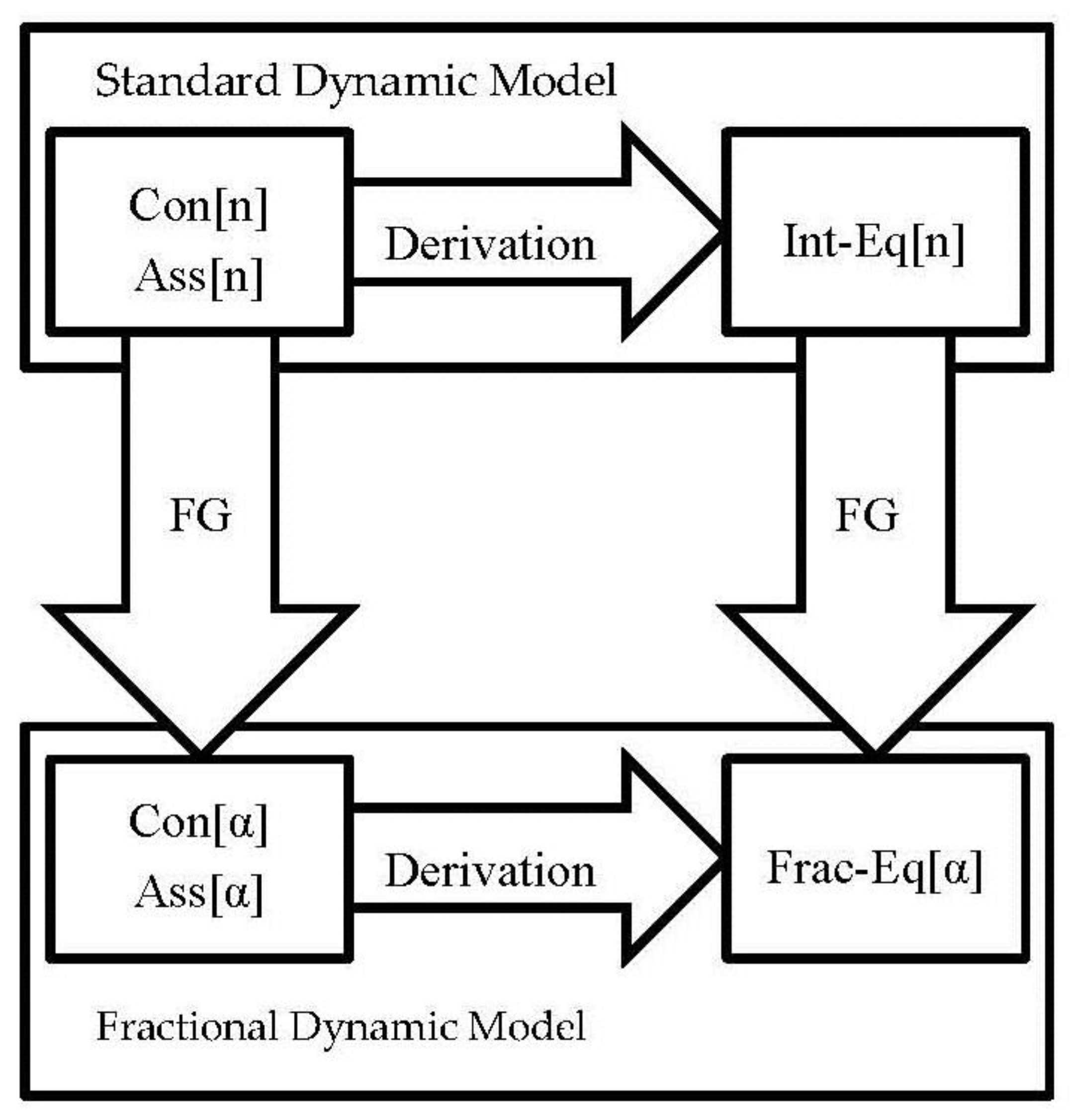
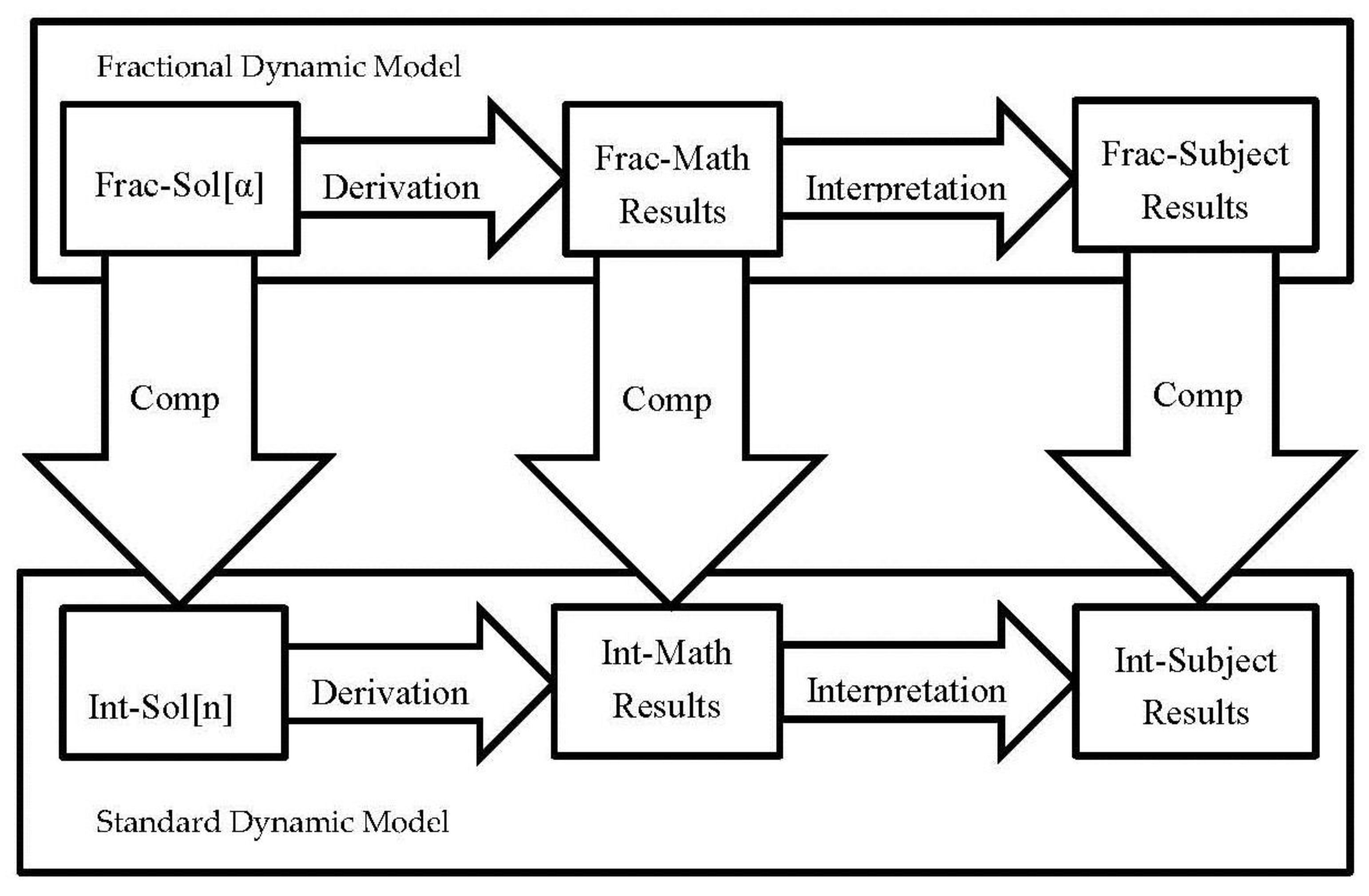
Derivability Principle:It is not enough to generalize the differential equations describing the dynamic model. It is necessary to generalize the whole scheme of obtaining (all steps of derivation) these equations from the basic principles, concepts and assumptions. In this sequential derivation of the equations we should take into account the non-standard characteristic properties of fractional derivatives and integrals. If necessary, generalizations of the notions, concepts and methods, which are used in this derivation, should also be obtained.

The derivability principle states that we should realize a correct fractional generalization of the derivation of the model equations. It is necessary to generalize not only and not so much the differential equation of the model itself, but a generalization of all steps of deriving the standard (non-fractional) equations of the model. In the general case, this will not be an equation that is obtained by simply replacing the integer derivatives with fractional derivatives of non-integer order. Often, the consistent construction of a fractional-dynamic model is associated with the need to introduce new concepts and notions that generalize the concepts and notions of standard models. Note that fractional generalizations of basic concepts are not so much a part of this particular model, but in fact are the common basis of different models, and basis of all fractional dynamics (fractional mathematical economics), and not just the model. An important part of this derivation is the need to take into account the non-standard characteristic properties of fractional derivatives and integrals [17,18,19,20,21,22]. These properties include (a) violation of the standard chain rule (for example, see [3], pp. 97–98, [5], pp. 35–36, [19] and Section 2.1); (b) violation of the standard semi-group property for orders of derivatives (see [1], pp. 46–47, [5], p. 30, and Section 2.2); (c) violation of the standard product (Leibniz) rule (for example, see [1], pp. 280–284, [3], pp. 91–97, [5], pp. 33, 59, [17,20,22] and Section 2.3); (d) violation of the standard semi-group property for dynamic maps (see the explanations and references in Section 2.4). These properties narrow the field for maneuver and make it difficult to obtain fractional generalizations. These non-standard properties are obstacles that must be overcome to build correct fractional dynamic models. At the same time, these non-standard properties allow us to get correct fractional dynamic models to describe non-standard effects, processes and phenomena. Schematically, this principle is represented by Figure 1.

(2)

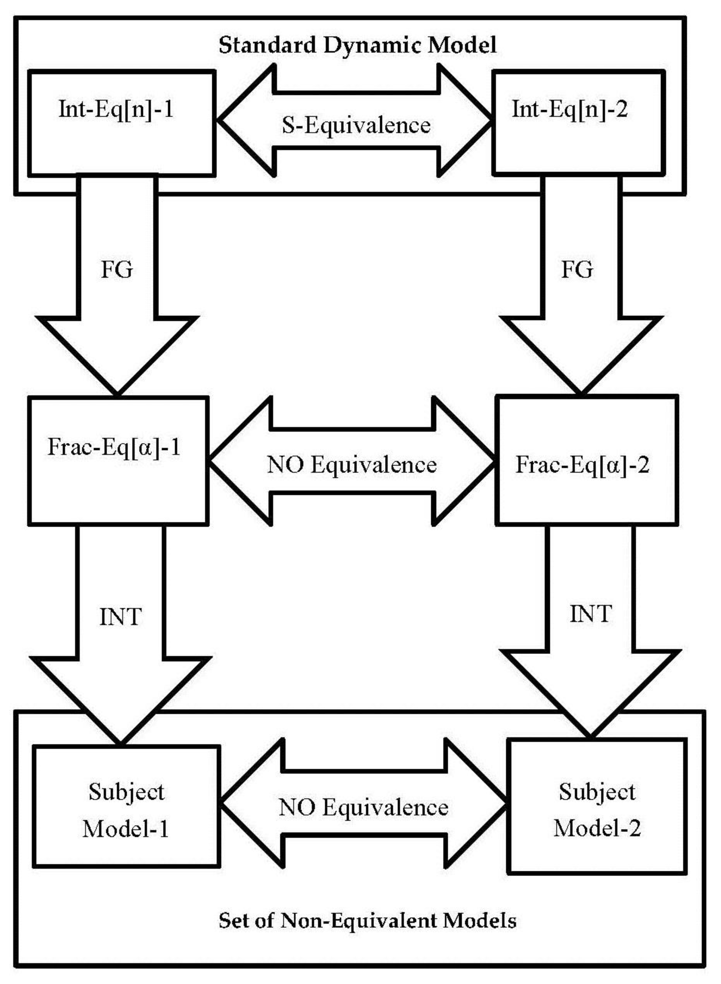
Multiplicity Principle:For one standard model, there is a set of fractional dynamical generalizations, due to the existence of various types of fractional operators and violation of s-equivalence for fractional differential equations.

In addition to existence a large number of different types of fractional derivatives and integrals, the violation of the standard rules generate an additional uncertainty of fractional generalizations. Fractional generalizations of solution-equivalent (s-equivalent) representations of integer-order differential equations of standard models, as a rule, lead to different fractional differential equations that have non-equivalent solutions. This situation is partially analogous to the fact that quantization of equivalent classical models leads to nonequivalent quantum theories. As a result, fractional generalizations of one standard model (which is represented by s-equivalent differential equations of integer order) can lead to different fractional-dynamic models that will predict different behaviors of a process and only some of them may be useful in a given context. We can state that for one standard model, there is a family of fractional dynamical generalizations, due to the existence of various types of fractional operators and violation of s-equivalence for fractional differential equations. In this regard, it is important to investigate and describe the properties of solutions of fractional dynamic equations, which are (qualitatively and/or quantitatively) the same, and the properties of solutions that are (first of all, qualitatively) different. Schematically, this principle is given by Figure 2.

(3)

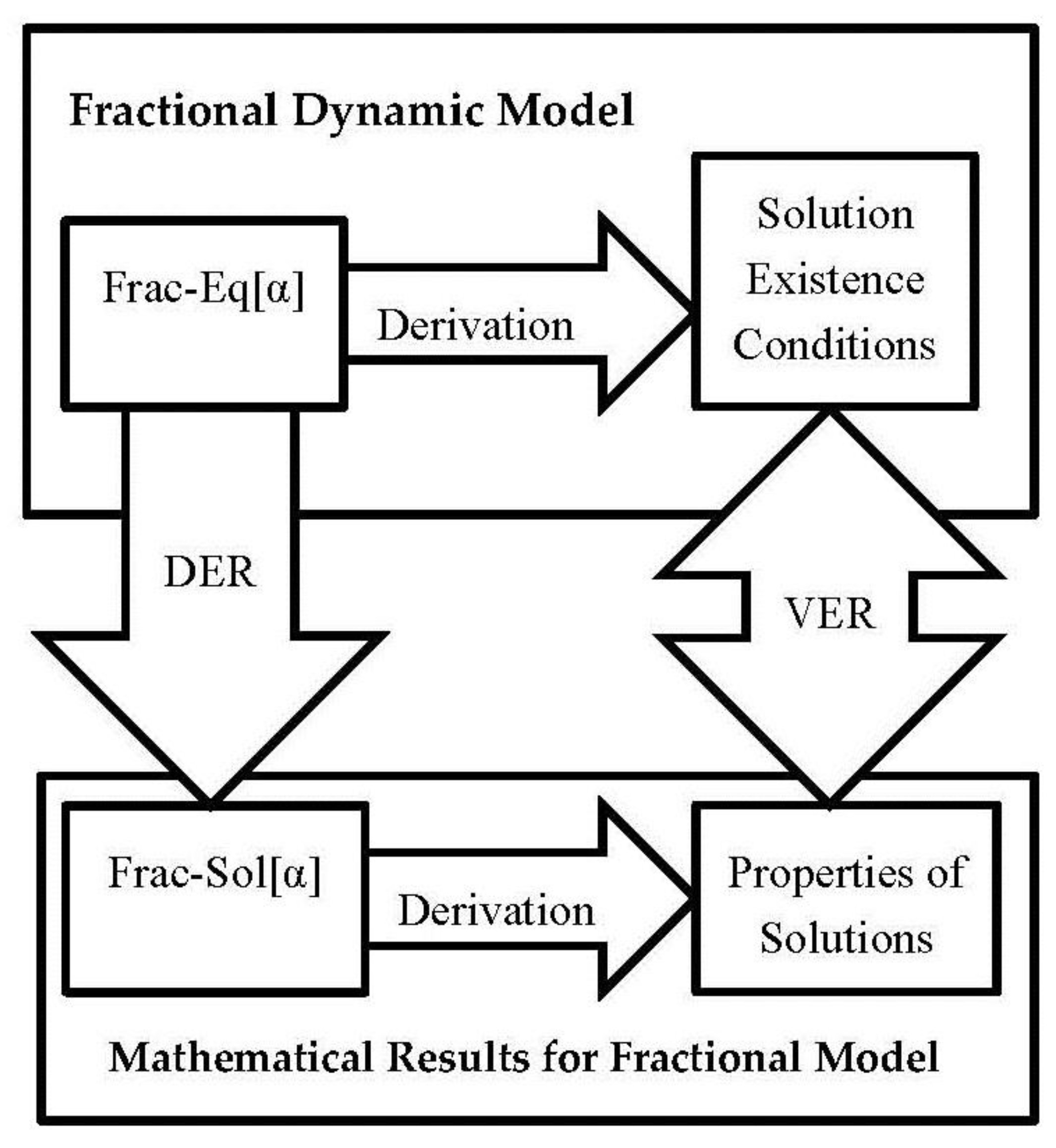
Solvability Principle:The properties of process types (such as long memory, spatial nonlocality, distributed delay, distributed scaling) and the properties of the corresponding types of fractional operators must be taken into account in the existence of solutions, and in obtaining correct analytical and numerical solutions.

The solvability principle states that the existence of solution, and the possibility of obtaining an exact analytical solution or correct numerical solutions for some conditions. Obviously, the existence conditions should allow us to obtain solutions for those cases and properties that the described process has. In addition, we should take into account that different types of fractional derivatives and integrals are known in fractional calculus [1,2,4]. Therefore, in fractional dynamic generalization, it is important that type of fractional operators correspond to the type of natural or social process. It should be noted that not all well-known fractional operators can describe the long memory and spatial non-locality (see Section 2.5 of this paper). For example, some fractional operators can be used to describe the distributed lag (time delay) and the distributed scaling (dilation) and they are not suitable for memory and non-locality. Additionally, we need to verify the existence condition for properties of solutions obtained. For example, if we describe processes with long memory then derivation of numerical solution must take into account not only local information, but the numerical scheme must contain memory terms. Schematically, this principle is represented by Figure 3.

(4)

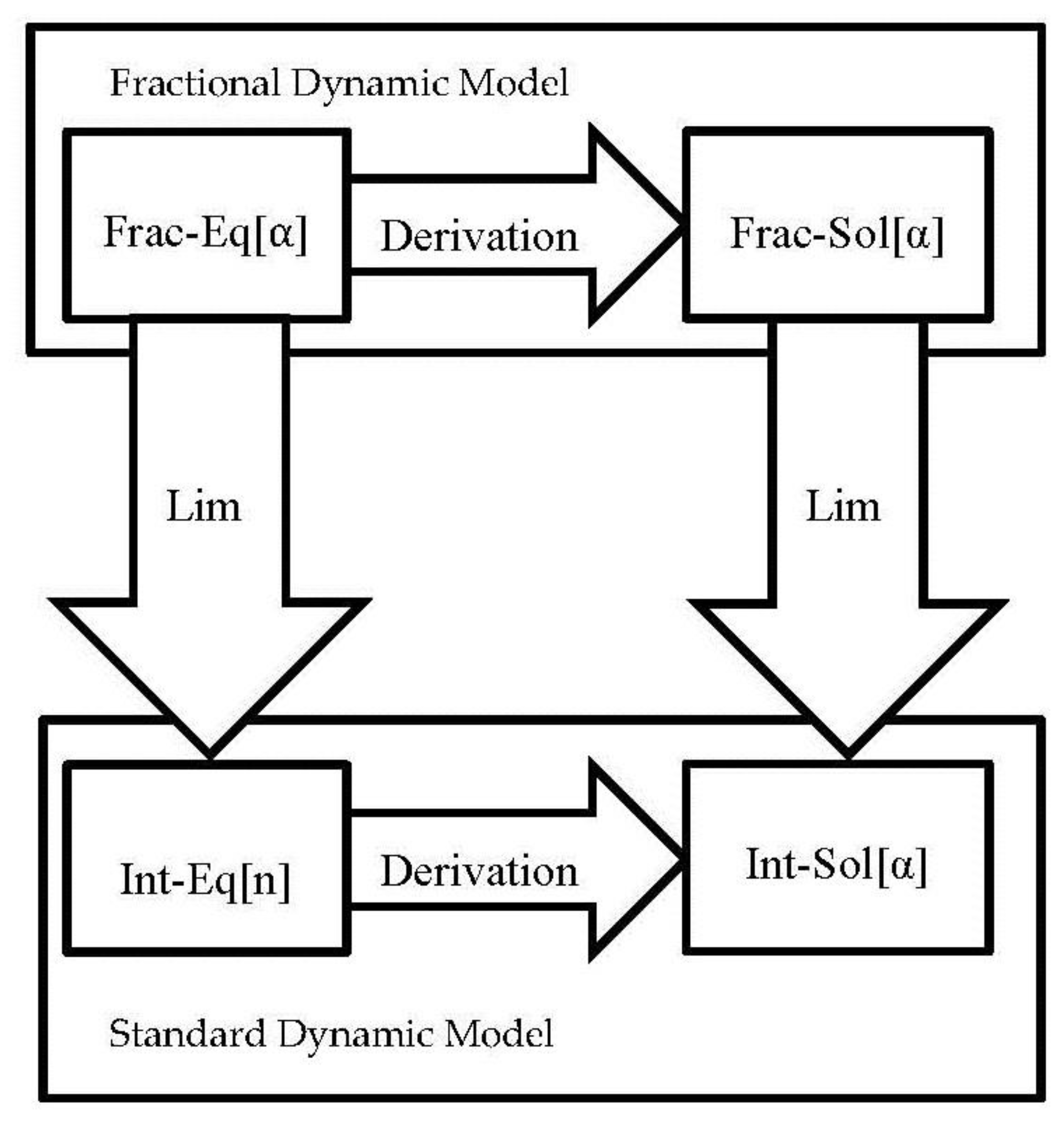
Correspondence Principle:The limiting procedure, when orders of fractional derivatives tend to integer values, applied to the equations of the fractional dynamic model and their solutions, should give the standard model equations and their solutions.

The correspondence principle means a possibility of obtaining equations and solutions of standard model by using a limit procedure, when the orders of the fractional derivatives tend to an integer values. The principle of correspondence must be fulfilled both for the equation itself and for its solution. It should be noted if the order of the derivative tends to the integer value, then the limit on the left and the limit on the right can give different results in the general case. Schematically, this principle is depicted in Figure 4.

The Correspondence Principle can also be represented by the formal expression:

$$\underset{\alpha \to n}{\lim }\mathrm{Frac}-\mathrm{Eq}\left[\mathsf{\alpha }\right]=\mathrm{Int}-\mathrm{Eql}\left[\mathrm{n}\right],$$

(1)

$$\underset{\alpha \to n}{\lim }\mathrm{Frac}-\mathrm{Sol}\left[\mathsf{\alpha }\right]=\mathrm{Int}-\mathrm{Sol}\left[\mathrm{n}\right],$$

(2)

where $n\in \mathbb{N}.$ It should be noted that the limit on the left and the limit on the right do not coincide in the general case:

$$\underset{\alpha \to n-}{\lim }\mathrm{Frac}-\mathrm{Sol}\left[\mathsf{\alpha }\right]\ne \underset{\alpha \to n+}{\lim }\mathrm{Frac}-\mathrm{Sol}\left[\mathsf{\alpha }\right].$$

(3)

(5)

Interpretability Principle:The subject (physical, economic) interpretation of the mathematical results, including solutions and its properties, should be obtained. Differences, and first of all qualitative differences, from the results based on the standard model should be described.

The subject interpretation of the solutions should be obtained. The properties of solutions should be described in details with their economic or physical meaning (interpretation). It is important to have an interpretability of mathematical results. The differences between results, which were obtained for the proposed generalization and the standard model, should be clearly indicated. An important purpose is to find qualitative differences between the properties of solutions for the fractional dynamic model and the properties of the solutions of the standard model. Schematically, this principle is given by Figure 5.

The proposed five principles are designed primarily to eliminate errors that are usually made when building fractional dynamic generalizations of standard models. The most important element is the requirement that in fractional generalization of economic (or physical) model the “output” of the research should be an economic (physical) conclusions (phenomena, effects) and new economic (physical) effects that are a consequence of subject assumptions on the “input”. Here, mathematics (fractional calculus) is the tool that mathematically strictly connects “economic/physical input” and “economic/physical output”. If mathematical equations and solutions are not rigidly connected with subject “input” and “output”, they will fly away into “airless space”. In this case, the results will turn from economics and physics into formal manipulations, which may not even have mathematical value from the point of view of pure mathematics (fractional calculus).

An important goal of fractional generalizations is to obtain qualitatively new effects and phenomena in natural and social sciences. The results obtained in a science by using the new mathematical apparatus (fractional calculus) should give qualitatively new results and predict new effects and phenomena for this science. First of all, it is precisely such qualitatively new results are interesting in the first place.

In this paper, we illustrate these rules (principles) by using examples of fractional generalizations of standard economic models.

In Section 2 of this paper, we describe the non-standard rules for fractional operators of non-integer orders. The violation of the standard chain rule is described in Section 2.1. The violation of the standard semi-group property for orders of derivatives is discussed in Section 2.2. We consider the violation of the standard product (Leibniz) rule in Section 2.3. The violation of the standard semi-group property for dynamic maps is described in Section 2.4. A correspondence between the types of fractional operators of non-integre orders and the types of phenomena is discussed in Section 2.5.

In Section 3, we consider an application of the Derivability Principle and we give examples of the problem with the violation of the standard rules for fractional operators of non-integer orders. In Section 3.1, to illustrate problems that are connected with the non-standard form of the chain rule, we consider a fractional generalization of the Kaldor-type model of business cycles. In Section 3.2, problem with violation of the standard semi-group rule for orders of derivatives is shown for the fractional generalization of the Phillips model of the multiplier-accelerator. In Section 3.3, to illustrate the problems arising from the non-standard form of the product (Leibniz) rule, we consider the fractional generalization of the standard Solow–Swan model. In Section 3.4, the problem with the violation of the standard semi-group property of dynamic map is described using the examples of fractional generalization of the dynamic Leontief (intersectoral) model and logistic growth model. In Section 3.4, the definitions of new economic concepts and notions are described.

In Section 4, the Solvability Principle and the Correspondence Principle are discussed and some examples are suggested. In Section 4.1, we discuss the Solvability Principle by using the general fractional calculus as an example. In Section 4.2, for illustration we consider the distributed lag fractional calculus and growth-relaxation equations with gamma distributed delay time. In Section 4.3, a simple example of the Correspondence Principle for the case, when the order of the derivative tends toward integer values from the left and from the right, is considered. In Section 4.4, the Solvability Principle is discussed by using example from numerical simulation of fractional differential equations.

In Section 5, we describe some problems (“Non-Equivalence” and “Unpredictability”) of fractional generalizations that are associated with non-equivalent fractional equations, which are formal generalization of equivalent differential equations of integer orders. In Section 5.1, we give definitions of equivalence of equations by solutions (s-equivalence). In Section 5.2, we illustrate non-equivalence of fractional generalization for relaxation and growth differential equations. In Section 5.3, we describe non-equivalence of fractional generalization of the fractional logistic equation that in economics describes growth in a competitive environment with memory. In Section 5.4, we formulate that fractional generalization of standard model can generate non-equivalent models.

In Section 6, we consider example of application of the Interpretability Principle by describing some examples of new effects and phenomena in economics. In Section 6.1, we describe a simple economic model with memory. Fractional differential equation, its solution and asymptotic behavior are proposed. In Section 6.2, we give an interpretation of the mathematical results by using suggested new concept of the warranted rate of growth with memory. In Section 6.3, we describe the interpretation of mathematical results in the form of economic phenomena for economic growth and decline with memory. In Section 6.4, we describe an interpretation of relaxation of economic processes with memory.

In Section 7, we give a short conclusion.

2. Non-Standard Properties of Fractional Derivatives

In this section we describe some properties (rules) of fractional derivatives causing problems when constructing fractional generalizations of standard dynamic models.

The fractional derivatives of non-integer orders have a set of non-standard properties and rules such as the violation of the standard product (Leibniz) and the standard chain rules, the violation of semigroup rules for orders of the derivatives and the violation of semigroup rules for dynamical map. The non-standard properties of fractional derivatives should be taken into account, when constructing fractional generalization of dynamic models. These properties create problems in realization of the derivability principle.

2.1. Violation of Standard Chain Rule

The standard chain rule for the first order derivative has the form:

$$D_t^{1}f\left(g\left(t\right)\right)={(D_g^{1}f\left(g\right))}_{g=g\left(\mathrm{t}\right)}{D}_t^{1}g\left(\mathrm{t}\right),$$

(4)

where $D_t^1=d/dt$ is the derivative of first order. The standard chain rule for the derivative of integer order $n\in \mathbb{N}$ can be written by the equation:

$$D_t^{n}f\left(g\left(\mathrm{t}\right)\right)=n!{\displaystyle \sum _{m=1}^n}{(D_g^{m}f\left(g\right))}_{g=g\left(t\right)}\sum {\displaystyle \prod _{r=1}^n}\frac{1}{a_r!}{\left(\frac{1}{r!}{D}_t^{r}g\left(\mathrm{t}\right)\right)}^{a_r},$$

(5)

which is called the Faá di Bruno’s formula [23].

The standard chain rules shown in Equations (4) and (5) are not satisfied for fractional derivatives of non-integer orders. Foe example, the chain rule for the Riemann–Liouville fractional derivative of the order $\alpha >0$ (see equation (2.209) in section 2.7.3 of [3], pp. 97–98, [5], pp. 35–36, and [19]) has the form:

$$\begin{array}{c}{D}_{RL,0+}^{\alpha }f\left(g\left(t\right)\right)=\frac{t^{\alpha }f\left(g\left(t\right)\right)}{\mathsf{\Gamma }\left(1-\alpha \right)}+\\ {\displaystyle \sum _{k=1}^{\infty }}{C}_k^{\alpha }\frac{k!t^{k-\alpha }}{\mathsf{\Gamma }\left(k-\alpha +1\right)}{\displaystyle \sum _{m=1}^k}{\left(D_g^{m}f\right(g\left)\right)}_{g=g\left(t\right)}\sum {\displaystyle \prod _{r=1}^k}\frac{1}{a_r!}{\left(\frac{1}{r!}{D}_t^{r}g\left(\mathrm{t}\right)\right)}^{a_r},\end{array}$$

(6)

where $t>0$, $D_g^m$ and $D_t^r$ are derivatives of integer orders, ∑ extends over all combinations of non-negative integer values of $a_1$, $a_2$, …, $a_k$ such that ${\sum }_{r=1}^{k}r{a}_r=k$ and ${\sum }_r^k{a}_r=m$.

The chain rules for other type of fractional derivatives have a similar form. We see that standard chain rules (4) and (5) do not satisfied for fractional derivatives of non-integer order.

2.2. Violation of Semi-Group Rule for Orders of Derivatives

The standard semi-group rule for orders of integer-order derivatives has the form of the equality:

$$D_t^n{D}_t^{m}X\left(t\right)=D_t^{n+m}X\left(t\right),$$

(7)

which holds for $n,m\in \mathbb{N}$, if the function $X\left(t\right)$ is smooth or $X\left(t\right)$ is a continuous function that has continuous first $n+m$ derivatives (for example, $X\left(t\right)\in C^{n+m}(ℝ)$). It is well known that this property may be broken for discontinuous functions $X\left(t\right)$ and if the derivatives are not continuous.

For fractional derivatives, the standard semi-group rule (7) is not satisfied in the general case (for example, see [1], pp. 46–47 and [5], p. 30). For example, the Caputo fractional derivatives of the orders $0<\alpha ,\beta <1$ satisfy the equality:

$$\left(D_{C,0+}^{\alpha }{D}_{C,0+}^{\beta }X\right)\left(t\right)=\left(D_{C,0+}^{\alpha +\beta }X\right)\left(t\right)+\frac{1}{\mathsf{\Gamma }\left(2-\alpha -\beta \right)}{X}^{\left(1\right)}\left(0\right)t^{1-\alpha -\beta },$$

(8)

where $D_{C,0+}^{\alpha }$ and $D_{C,0+}^{\beta }$ are the Caputo fractional derivative of the orders $0<\alpha ,\beta <1$ is defined by the equation:

$$\left(D_{0+}^{\alpha }X\right)\left(t\right)=\frac{1}{\mathsf{\Gamma }\left(1-\alpha \right)}{{\displaystyle \int }}_0^t{\left(t-\tau \right)}^{-\alpha }{X}^{\left(1\right)}\left(\tau \right)d\tau ,$$

(9)

where $\mathsf{\Gamma }\left(\alpha \right)$ is the gamma function. Equality (8) means the violation of the semi-group property for orders of derivatives, i.e., in general, we have the inequality:

$$\left(D_{C,0+}^{\alpha }{D}_{C,0+}^{\beta }X\right)\left(t\right)\ne \left(D_{C,0+}^{\alpha +\beta }X\right)\left(t\right),$$

(10)

if the orders of these fractional derivatives are non-integer. In the order $\alpha$ of the Caputo fractional derivative in (10) is non-integer and the order $\beta =n\in \mathbb{N}$, then we have the equality $\left(D_{C,0+}^{\alpha }{D}_t^{n}X\right)\left(t\right)=\left(D_{C,0+}^{\alpha +n}X\right)\left(t\right).$ If the order $\alpha =n\in \mathbb{N}$ and $\beta$ is non-integer, then the standard semi-group property is violated, i.e., the inequality $\left(D_t^n{D}_{C,0+}^{\beta }X\right)\left(t\right)\ne \left(D_{C,0+}^{n+\beta }X\right)\left(t\right)$ holds in general.

2.3. Violation of the Standard Product Rule

The standard product (Leibniz) rule for first-order derivative $\left(\mathrm{for}n=1\right)$ has the form:

$$D_t^1\left(f\left(\mathrm{t}\right)g\left(\mathrm{t}\right)\right)=\left(D_x^1\mathrm{f}\left(x\right)\right)g\left(x\right)+f\left(x\right)\left(D_x^{1}g\left(x\right)\right).$$

(11)

The standard product rule for the derivative of integer order $n\in \mathbb{N}$ has the form:

$$D_t^n\left(f\left(t\right)g\left(t\right)\right)={\displaystyle \sum _{k=0}^n}\frac{n!}{\left(n-k\right)!k!}\left(D_t^{n-k}f\left(t\right)\right)\left(D_t^{k}g\left(t\right)\right).$$

(12)

The Leibniz rule for derivative of non-integer order $\alpha \ne 1$ cannot have the simple form:

$$D_t^{\alpha }\left(f\left(t\right)g\left(t\right)\right)=\left(D_t^{\alpha }f\left(t\right)\right)g\left(t\right)+f\left(t\right)\left(D_t^{\alpha }g\left(t\right)\right).$$

(13)

A violation of relation in Equation (13) is a characteristic property of all derivatives of integer-orders $n\in \mathbb{N}$ greater than one and for all types derivatives of the non-integer order $\alpha >0$ (for example, see [1], pp. 280–284, [3], pp. 91–97, [5], p. 33, 59, and [17,20,22]). In [17], the following theorem has been proved:

Theorem 1

(“No violation of the Leibniz rule. No fractional derivative”).If a linear operator$D_t^{\alpha }$satisfiesthe product rule in the form of Equation (13), then the operator$D_t^{\alpha }$is the differential operator of first order, that can be represented in the form$D_t^{\alpha }=a\left(t\right)D_t^1$, where$a\left(t\right)$is function on$ℝ$.

As a result, we can states that derivatives of non-integer orders $\alpha \ne 1$ cannot satisfy the standard product rule of Equation (13). For example, the fractional generalization of the Leibniz rule for the Riemann–Liouville derivatives has the form (see section 15 in [1], pp. 277–284), of the infinite series:

$$D_{RL}^{\alpha }\left(f\left(t\right)g\left(t\right)\right)={\displaystyle \sum _{k=0}^{\infty }}\frac{\mathsf{\Gamma }\left(\alpha +1\right)}{\mathsf{\Gamma }\left(\alpha -k+1\right)\mathsf{\Gamma }\left(k+1\right)}\left(D_{RL}^{\alpha -k}f\left(t\right)\right)\left(D_t^{k}g\left(t\right)\right),$$

(14)

where $f\left(\mathrm{t}\right)$ and $g\left(\mathrm{t}\right)$ are analytic functions on [a, b] (see theorem 15.1 in [1]), $D_{RL}^{\alpha }$ is the Riemann–Liouville derivative; $D^k$ is derivative of integer order $k\in \mathbb{N}$. It should be noted that the sum of Equation (14) is infinite and it contains the fractional integrals $I_{RL}^{k-\alpha }=D_{RL}^{\alpha -k}$ of non-integer orders $\left(k-\alpha \right)$ for the values $k>\left[\alpha \right]+1$.

2.4. Violation of the Standard Semi-Group Rule for Dynamic Maps

Let us consider linear ordinary differential equation equations of first order in the form:

$$\frac{dX\left(t\right)}{dt}=AX\left(t\right),$$

(15)

where $X\left(t\right)$ is an unknown function (with values in a Banach space) and $A$ is a constant linear bounded operator acting in the space (or $A$ is the linear operator having an everywhere dense domain of definition $D\left(A\right)$ in the Banach space). We can consider the Cauchy problem of finding a solution of Equation (15) for $0<t<\infty ,$ satisfying the given initial condition $X\left(0\right)=X_0\in D\left(A\right)$. A unique solution of the Cauchy problem exists for the differential equation of first order (Equation (15)) with a constant bounded operator $A$ and it can be written (for example, see [24], pp. 119–157) in the form:

$$X\left(t\right)=U\left(t\right)X\left(0\right),$$

(16)

where the operator $U\left(t\right)$ is defined by the series:

$$U\left(t\right)=exp\left(tA\right)={\displaystyle \sum _{k=0}^{\infty }}\frac{t^k}{k!}{A}^k,$$

(17)

which converges in the operator norm. The operator $U\left(t\right)$ is called the dynamic map or the phase flow [25].

A family of bounded linear operators $U\left(t\right)$, depending on the parameter $0<t<\infty ,$ forms a semi-group if the condition $U\left(0\right)=I$ and the equality:

$$U\left(t_1\right)U\left(t_2\right)=U\left(t_1+t_2\right)$$

(18)

hold for all $t_1,t_2$ where $0<t_1,t_2<\infty .$ Equation (18) is the standard semi-group rule for dynamical map. The set $\{U\left(t\right),t>0\}$ is called one-parameter dynamical semi-group. In quantum theory the operator $A$ is called the infinitesimal generator of the quantum dynamical semi-group (see classical papers [26,27,28,29]). The class of differential equations for which $A$ is a generator for a semigroup of class ($C_0$) coincides with the class of differential equations for which the Cauchy problem is uniformly correct [24].

Daftardar-Gejji and Babakhani [30] (see also [31] and [4], p. 142) have studied the existence, uniqueness, and stability of solutions for the fractional differential equations:

$$\left(D_{C,0+}^{\alpha }X\right)\left(t\right)=AX\left(t\right),$$

(19)

where $D_{C,0+}^{\alpha }$ is the Caputo fractional derivative of the order $0<\alpha <1$, $X\left(t\right)$. is the column vector and $A$. is real square $NxN$ matrix. They obtained the unique solution of Equation (19) in the form:

$$X\left(t\right)=U_{\alpha }\left(t\right)X\left(0\right),$$

(20)

where the operator $U_{\alpha }\left(t\right)$ is defined by the series:

$$U_{\alpha }\left(t\right)=E_{\alpha }\left[t^{\alpha }A\right]={\displaystyle \sum _{k=0}^{\infty }}\frac{{\left(t^{\alpha }\right)}^k}{\mathsf{\Gamma }\left(\alpha k+1\right)}{A}^k.$$

(21)

Here, $E_{\alpha }\left[t^{\alpha }A\right]$ is the Mittag–Leffler function with matrix arguments [32].

For $\alpha =1$, we have $E_1\left[z\right]=exp\left(z\right)$. Therefore, we have $U_1\left(t\right)=U\left(t\right)=exp\left(tA\right)$.

The standard semi-group rule (Equation (18)) for dynamical maps $U_{\alpha }\left(t\right)$ does not hold for non-integer values of $\alpha \in \left(0,1\right)$, i.e., we have the inequality:

$$U_{\alpha }\left(t_1\right)U_{\alpha }\left(t_2\right)\ne U_{\alpha }\left(t_1+t_2\right)$$

(22)

that follows from the property of the Mittag–Leffler function (for example, see [33,34], and some additional information in [35,36,37]) in the form:

$$E_{\alpha }\left[t_1^{\alpha }A\right]E_{\alpha }\left[t_2^{\alpha }A\right]\ne E_{\alpha }\left[{\left(t_1+t_2\right)}^{\alpha }A\right].$$

(23)

As a result, the dynamical maps $U_{\alpha }\left(t\right)$ with $\alpha \notin \mathbb{N}$ cannot form a semigroup.

The operator $U_{\alpha }\left(t\right)$ describes the dynamical map with power-law fading memory for non-integer values of $\alpha$. The violation of the standard semigroup rule for dynamical maps is a characteristic property of dynamics with memory. We can only state that the set $\{U_{\alpha }\left(t\right),t>0\}$ of the dynamical map with memory forms a dynamical groupoid [34,37] for on-integer values of $\alpha \in \left(0,1\right)$.

It should be noted that the fractional differential Equation (19) describes the fractional generalization of N-level open quantum system and the Leontief dynamic model of N-sectors in economy, in which the power-law memory is taken into account (see Section 3.4.1).

2.5. What Effects Are Fractional Derivatives Described?

In fractional calculus, many different types of fractional derivatives and integrals are known [1,2,3,4]. In construction of a fractional generalization of a standard dynamic model, an important part of the work is an adequate choice of the type of the fractional derivative or/and integral. First of all, fractional operators must correspond to the type of process to be described. It is well known that fractional derivatives and integrals are a powerful tool for describing processes with memory and nonlocality. However, not all fractional operators can describe the effects of memory (or non-locality). In application of the generalized and general fractional operators, an important question arises about the correct subject interpretation of these operators (for example, see informational [38], physical [39], and economic [40,41,42] interpretations). It is important to emphasize that not all fractional operators can describe the processes with memory (for example, see [43,44,45,46]). It is important to clearly understand what type of phenomena a given operator can describe. Let us give some examples for illustration.

2.5.1. First Example: Kober and Erdelyi–Kober Operators

The Kober fractional integration of non-integer order [1,2,4] can be interpreted as an expected value of a random variable up to a constant factor (for example, see [43,45] and section 10 in [46]), where the random variable describes scaling (dilation) with the gamma distribution. The Erdelyi–Kober integral operator, the differential operators of Kober and Erdelyi–Kober type have analogous interpretation [43,45,46]. As a result, these operators are integer-order operator with continuously distributed scaling (dilation), and these operators cannot describe the memory. Note that the fractional generalizations of the Kober and Erdelyi–Kober operators, which can be used to describe memory and distributed scaling (dilation) simultaneously, were proposed in [46].

The Kober fractional integral of the order $\alpha >0$ [4], p. 106, is defined as:

$$\left(I_{K;0+;\eta }^{\alpha }\phi \right)\left(t\right)=\frac{t^{-\alpha -\eta }}{\mathsf{\Gamma }\left(\alpha \right)}{{\displaystyle \int }}_0^t{\tau }^{\eta }{\left(t-\tau \right)}^{\alpha -1}\phi \left(\tau \right)d\tau ,$$

(24)

where $\mathsf{\alpha }>0$ is the order of integration and $\eta \in ℝ$. Using the variable $x=\tau /t$, this operator can be represent by the equation:

$$\left(I_{K;0+;\eta }^{\alpha }\phi \right)\left(t\right)=\frac{\mathsf{\Gamma }\left(\eta +\alpha +1\right)}{\mathsf{\Gamma }\left(\eta +1\right)}{{\displaystyle \int }}_0^1{f}_{\eta +1;\alpha }\left(x\right)\left(S_x\phi \right)\left(t\right)dx,$$

(25)

where $S_x$ is the operator [1], pp. 95–96 and [4], p. 11 such that $\left(S_x\phi \right)\left(t\right)=\phi \left(xt\right)$ and $f_{\alpha ;\beta }\left(x\right)$ is the probability density function (pdf) of the beta-distribution such that:

$$f_{\alpha ;\beta }\left(x\right)=\frac{1}{B\left(\alpha ,\beta \right)}{x}^{\alpha -1}{\left(1-x\right)}^{\beta -1}$$

(26)

for $x\in \left[0,1\right]$ and $f_{\alpha ;\beta }\left(x\right)=0$ if $x\notin \left[0,1\right]$, where $B\left(\alpha ,\beta \right)$ is the beta function. We see that the Kober integral operator describes beta distributed scaling up to numerical factor. For details see [43,45] and section 10 in [46].

2.5.2. Second Example: Causality Principle and Kramers–Kronig Relations

To describe processes with memory [47,48,49], the operators should satisfy the causality principle. For natural and social processes with memory, the causality can be described by the Kramers–Kronig relations [50]. The Riesz fractional operators (see section 2.10 of [4]) cannot be used to describe memory since this operator violates the causality principle. The Riesz fractional operators can be used to describe power-law non-locality and power-law spatial dispersion (for example, see [51,52]).

The principle of causality is represented in the form of the Kramers–Kronig relations (the Hilbert transform pair) by using the Fourier transforms. Let us consider the Fourier transform $\tilde{M}\left(\omega \right)$ of the memory function $M\left(t\right)$. In general, $\tilde{M}\left(\omega \right)$ is the complex function $\tilde{M}\left(\omega \right)={\tilde{M}}_1\left(\omega \right)+i{\tilde{M}}_2\left(\omega \right),$ where the real part ${\tilde{M}}_1\left(\omega \right)=Re\left[\tilde{M}\left(\omega \right)\right]$ and the imaginary part ${\tilde{M}}_2\left(\omega \right)=Im\left[\tilde{M}\left(\omega \right)\right]$ are real-valued functions. The Kramers–Kronig relations state that the real part and the imaginary parts of the memory function are not independent, and the full function can be reconstructed given just one of its parts. Let us assume that the function $\tilde{M}\left(\omega \right)$ is analytic in the closed upper half-plane of frequency $\mathsf{\omega }$ and vanishes like $1/\left|\mathsf{\omega }\right|$ or faster as $\left|\mathsf{\omega }\right|\to \infty$. The Kramers–Kronig relations are given by:

$${\tilde{M}}_1\left(\omega \right)=\frac{1}{\pi }P.V.{\displaystyle \underset{-\infty }{\overset{+\infty }{{\displaystyle \int }}}}\frac{1}{\mathsf{\Omega }-\omega }{\tilde{M}}_2\left(\mathsf{\Omega }\right)d\mathsf{\Omega },$$

(27)

$${\tilde{M}}_2\left(\omega \right)=-\frac{1}{\pi }P.V.{\displaystyle \underset{-\infty }{\overset{+\infty }{{\displaystyle \int }}}}\frac{1}{\mathsf{\Omega }-\omega }{\tilde{M}}_1\left(\mathsf{\Omega }\right)d\mathsf{\Omega },$$

(28)

where $\mathrm{P}.\mathrm{V}.$ denotes the Cauchy principal value. For details see [50].

2.5.3. Third Example: Abel-type Operator with Kummer Function in Kernel

The Abel-type fractional integral (and differential) operator with Kummer function (or the three parameter Mittag–Leffler functions) in the kernel (see the classic book [1] and equation (37.1) in [1], p. 731) can be interpreted as the Riemann–Liouville fractional integral (and derivatives) with gamma distribution of delay time [43,53,54].

It is known that the Abel-type (AT) fractional integral operator with Kummer function in the kernel (see equation (37.1) in [1], p. 731) is defined by the equation:

$$\left({\mathit{I}}_{\mathit{A}\mathit{T};\mathbf{0}+}^{\mathit{\alpha },\mathbf{\beta },\mathbf{\gamma },}Y\right)\left(t\right)=\frac{1}{\mathsf{\Gamma }\left(\alpha \right)}{{\displaystyle \int }}_0^t{\left(t-\tau \right)}^{\alpha -1}{F}_{1,1}\left(\beta ;\alpha ;\gamma \left(t-\tau \right)\right)Y\left(\tau \right)d\tau ,$$

(29)

and $F_{1,1}\left(a;b;z\right)$ is the confluent hypergeometric Kummer function. Using equality $F_{1,1}\left(a;c;z\right)=\mathsf{\Gamma }\left(c\right)E_{1,c}^a\left(z\right)$ the memory kernel in Equation (29) can be expressed through the three parameter Mittag–Leffler functions $E_{\alpha ,\beta }^{\gamma }\left(z\right)$.

The fractional integration with the gamma distributed lag in the form:

$$\left({\mathit{I}}_{\mathit{T};\mathit{R}\mathit{L};\mathbf{0}+}^{\mathit{\lambda },\mathit{a};\mathit{\alpha }}Y\right)\left(t\right)=\left(M_T^{\lambda ,a}\left(\tau \right)\ast \left(I_{RL,0+}^{\alpha }Y\right)\right)\left(t\right)={{\displaystyle \int }}_0^t{M}_T^{\lambda ,a}\left(\tau \right)\left(I_{RL,0+}^{\alpha }Y\right)\left(t-\tau \right)d\tau ,$$

(30)

where * denotes the Laplace convolution, $\left(I_{RL,0+}^{\alpha }Y\right)\left(t\right)$ is the Riemann–Liouville fractional integral [1,4], $M_T^{\lambda ,a}\left(\tau \right)$ is the probability density function (weighting functions) of the gamma distribution:

$$M_T^{\lambda ,a}\left(\tau \right)=\frac{{\lambda }^a{\tau }^{a-1}}{\mathsf{\Gamma }\left(a\right)}exp\left(-\lambda \tau \right)$$

(31)

for $\tau >0$ and $M_T^{\lambda ,a}\left(\tau \right)=0$ for $\tau \le 0$, where $a>0$ is the shape parameter and $\mathsf{\lambda }>0$ is the rate parameter. Equation (30) can be written thought the Laplace convolution of memory and weighting functions:

$$\left({\mathit{I}}_{\mathit{T};\mathit{C};\mathrm{0}+}^{\mathit{\lambda },\mathit{a};\mathit{\alpha }}Y\right)\left(t\right)=\left(M_T^{\lambda ,a}\ast \left(M_{RL}^{\alpha }\ast Y\right)\right)\left(t\right),$$

(32)

where $M_{RL}^{\alpha }\left(t\right)={\left(t-\tau \right)}^{\alpha -1}/\mathsf{\Gamma }\left(\alpha \right)$ is the kernel of the Riemann–Liouville fractional integral. The associativity of the Laplace convolution allows us to represent operator in the form:

$$\left({\mathit{I}}_{\mathit{T};\mathit{C};\mathrm{0}+}^{\mathit{\lambda },\mathit{a};\mathit{\alpha }}Y\right)\left(t\right)={{\displaystyle \int }}_0^t{M}_{TRL}^{\lambda ,a;\alpha }\left(t-\tau \right)Y\left(\tau \right)d\tau ,$$

(33)

where $M_{TRL}^{\lambda ,a;\alpha }\left(t\right)=\left(M_T^{\lambda ,a}\ast M_{RL}^{\alpha }\right)\left(t\right)$ is the memory-and-lag function of the form:

$$M_{TRL}^{\lambda ,a;\alpha }\left(t\right)=\frac{{\lambda }^a\mathsf{\Gamma }\left(a\right)}{\mathsf{\Gamma }\left(a+n-\alpha \right)}{t}^{a+\alpha -1}{F}_{1,1}\left(a;a+\alpha ;-\lambda t\right),$$

(34)

where $F_{1,1}\left(a;b;z\right)$ is the confluent hypergeometric Kummer function.

As a result, we obtain the relation:

$$\left({\mathit{I}}_{\mathit{A}\mathit{T};\mathbf{0}+}^{\mathit{a}+\mathit{\alpha },\mathit{a},-\mathit{\lambda },}Y\right)\left(t\right)=\frac{1}{{\lambda }^a\mathsf{\Gamma }\left(a\right)}.\left(I_{\mathit{T};\mathit{R}\mathit{L};\mathbf{0}+}^{\mathit{\lambda },\mathit{a};\mathit{\alpha }}Y\right)\left(t\right).$$

(35)

This equation shows that the AT fractional integral can be expressed through the Riemann–Liouville fractional integral with gamma distributed lag for wide range of parameters.

2.5.4. Fourth Example: Abel-type Operator with Kummer Function in Kernel

In application it is important to have conditions for the operator kernel, which make it possible to assign this operator to one or another type of phenomena or processes. For example, it is obvious that the kernels of general fractional convolution operators satisfying the normalization condition will describe distributed delays in time (lag), and not memory (for example, see [44,46], and some additional comments in [53,54,55]). It is well known in physics that the time delay is related to the finite speed of the process and not to the memory. For example, the Caputo–Fabrizio operators, which were misinterpreted as fractional derivatives of non-integer orders, are integer-order derivatives with the exponentially distributed delay time [43,44]. Therefore, these operators cannot be used to describe processes with memory. Note that the fractional derivatives with exponentially distributed is suggested in [43] and then applied in economics [53,54,55].

2.5.5. Fifth Example: Fractional operators with Uniform Distributed Order

The continual fractional derivatives and integrals were proposed by A.M. Nakhushev [56,57]. The fractional operators, which are inversed to the continual fractional integrals and derivatives, have been proposed by A.V. Pskhu [58,59]. In papers [47,60], we proved that the fractional integrals and derivatives of the uniform distributed order can be expressed (up to a numerical factor) thought the continual fractional integrals and derivatives that were suggested by A.M. Nakhushev. Therefore, the proposed fractional integral and derivatives of uniform distributed order we called in our paper [60] as the Nakhushev fractional integrals and derivatives. The corresponding inverse operators, which contain the two parameter Mittag–Leffler functions in the kernel, were called as the Pskhu fractional integrals and derivatives [60].

For example, the Riemann–Liouville fractional integral of distributed order is defined as:

$$\left(I_{RL,0+}^{\left[{\alpha }_1,{\alpha }_2\right]}X\right)\left(t\right)={{\displaystyle \int }}_{{\alpha }_1}^{{\alpha }_2}\rho \left(\alpha \right)(I_{RL,0+}^{\alpha }X)\left(t\right)d\alpha ,$$

(36)

where ${\mathsf{\alpha }}_2>{\mathsf{\alpha }}_1\ge 0$, and the weight function ρ(α) satisfies the normalization condition:

$${{\displaystyle \int }}_{{\alpha }_1}^{{\alpha }_2}\rho \left(\alpha \right)d\alpha =1.$$

(37)

In Equation (36) the integration with respect to time and the integration with respect to order can be permuted for a wide class of functions $X\left(\tau \right)$. As a result, Equation (36) is written in the form:

$$\left(I_{RL,0+}^{\left[{\alpha }_1,{\alpha }_2\right]}X\right)\left(t\right)={{\displaystyle \int }}_0^t{M}_{\rho \left(\alpha \right)}^{\left[{\alpha }_1,{\alpha }_2\right]}\left(t-\tau \right)X\left(\tau \right)d\tau ,$$

(38)

where the kernel $M_{\rho \left(\alpha \right)}^{\left[{\alpha }_1,{\alpha }_2\right]}\left(t-\tau \right)$ is defined by the equation:

$$M_{\rho \left(\alpha \right)}^{\left[{\alpha }_1,{\alpha }_2\right]}\left(t-\tau \right)={{\displaystyle \int }}_{{\alpha }_1}^{{\alpha }_2}\frac{\rho \left(\alpha \right)}{\mathsf{\Gamma }\left(\alpha \right)}\frac{1}{{\left(t-\tau \right)}^{1-\alpha }}d\alpha ,$$

(39)

where ${\mathsf{\alpha }}_2>{\mathsf{\alpha }}_1\ge 0$. In the simplest case, we can use the continuous uniform distribution (CUD) that is defined by the expression:

$$\rho \left(\alpha \right)=\{\begin{array}{c}\frac{1}{{\alpha }_2-{\alpha }_1}\\ 0\end{array}\begin{array}{c}for\alpha \in \left[{\alpha }_1,{\alpha }_2\right]\\ for\alpha \in \left(-\infty ,{\alpha }_1\right)\cup \left({\alpha }_2,\infty \right)\end{array}.$$

(40)

For the probability density function (Equation (40)), the memory function (Equation (39)) has the form:

$$M_{CUD}^{\left[{\alpha }_1,{\alpha }_2\right]}\left(t\right)=W\left({\alpha }_1,{\alpha }_2,t\right)=\frac{1}{\left({\alpha }_2-{\alpha }_1\right)t}{{\displaystyle \int }}_{{\alpha }_1}^{{\alpha }_2}\frac{t^{\xi }d\xi }{\mathsf{\Gamma }\left(\xi \right)}.$$

(41)

As a result, the fractional integral of uniform distributed order is defined by the equation:

$$I_{N,RL}^{\left[\alpha ,\beta \right]}X\left(t\right)=\frac{1}{\beta -\alpha }{{\displaystyle \int }}_{\alpha }^{\beta }\left(I_{RL,0+}^{\xi }X\right)\left(t\right)d\xi ={{\displaystyle \int }}_0^{t}W\left(\alpha ,\beta ,t-\tau \right)X\left(\tau \right)d\tau ,$$

(42)

where $\beta >\alpha >0$. The fractional integrals and derivatives of the uniform distributed order can be expressed thought the continual fractional integrals and derivatives, which have been suggested by A.M. Nakhushev [56,57].

2.5.6. Sixth Example: Left-Sided and Right-Sided Fractional Operators

The right-sided Riemann–Liouville, Liouville, and Caputo fractional derivatives [4] cannot describe the memory processes. Using only the left-sided derivatives of bon-integer orders, we take into account the history of changes of variable in the past, that is for $\tau <t$. The right-sided operators are defined by integration over $\tau >t,$ where $t$is the present moment of time. Using right-sided operators actually means that the present state depends on the future states, and not on the past states of the process.

2.5.7. Seventh Example: Fading Memory, Spetial Non-Locality, Time Delay (Lag), Scaling

Fractional calculus approach allows us to describe the spatial non-locality and fading memory of power-law type, the openness of processes and systems, intrinsic dissipation, long-range interactions, and some other type of phenomena. The most well-known phenomena in physics that can be described by fractional differential equations, are the fractional relaxation-oscillation, fractional diffusion-wave, fractional viscoelasticity, spatial and frequency dispersion of power type, nonexponential relaxation, anomalous diffusion, and some others [61,62].

As a result, we can state that the following type of phenomena can be independent of each other:

• fading memory (forgetting) (for example, see [47,48,49,50] and references therein) and power-law frequency dispersion;
• spatial non-locality (for example, see [63]) and power-law spatial dispersion (for example, see [64]);
• lag (time delay) (for example, see [43,53,54,55,65] and references therein); and
• scaling (dilation) (for example, see section 9 in [43] and references therein).

As a result, these phenomena are described by certain types of operator kernels. For other types of processes and phenomena, we do not have mathematical conditions on the kernel of operators, which allow us to uniquely identify one or another type of process. In this part of applied mathematics, the fractional calculus requires its development. Mathematically strict conditions on the operator kernels are necessary to initially distinguish between various types of processes and phenomena. It should be emphasized that we must first clearly distinguish between the types of processes and phenomena, but simply list various examples of their specific manifestations in the reality surrounding us, described by the natural and social sciences. It is necessary to establish a clear correspondence between the types of operator kernels and the types of phenomena.

3. Examples of Problems from Non-Standard Properties of Fractional Derivatives

In this section, we present examples illustrating the problems and difficulties of fractional generalization of standard dynamic models, which arise from non-standard properties of fractional derivatives. As an example of the problem with the non-standard form of the chain rule, we consider a fractional generalization of the Kaldor-type model of business cycles. Problem with the violation of the standard semi-group rule for orders of derivatives is shown for the fractional generalization of the Phillips model of the multiplier-accelerator. To illustrate the problems arising from the non-standard form of the product (Leibniz) rule, we consider the fractional generalization of the standard Solow–Swan model. Problem with the violation of the standard semi-group property of dynamic map is described on the examples of fractional generalization of the dynamic Leontief (intersectoral) model and logistic growth model.

3.1. Example of Problems with Chain Rule: Kaldor-Type Model of Business Cycles and Slutsky Equation

In this subsection, we demonstrate that the violation of the standard chain rule gives a restriction in fractional generalization of dynamic models. For this purpose, we consider a fractional generalization of the Kaldor-type model of business cycles and the economic model [66,67,68] based on the van der Pol equation [69,70].

Economic models, which are based on the van der Pol equation, are considered as prototypes of model for complex economic dynamics [69,70]. Nonlinear dynamic models are used to explain irregular and chaotic behavior of complex economic and financial processes (for example, see the business cycle theory [71,72], nonlinear economic dynamics and chaos [73,74], and stabilization [75]). Some models of business cycles, which are based on the Kaldor nonlinear investment-savings functions [69,70,71,72] and the Goodwin nonlinear accelerator-multiplier (for example, see the Goodwin’s paper [76], and [77,78,79]), can be reduced to the van der Pol equation, which describes damped oscillations [69,70,71,72].

3.1.1. Standard Kaldor-Type Model of Business Cycles

In the framework of Keynesian approach to theory of national income, Nicholas Kaldor formulated [66,67,68] the first nonlinear model of endogenous business cycles in 1940. Kaldor consider the interactions between the investment $I\left(Y\right)$ and the savings $S\left(Y\right)$, where $Y=Y\left(t\right)$ denotes national income. Using the fact that the linear functions $I\left(Y\right)$ and $S\left(Y\right)$ cannot describe processes of business cycle, Kaldor proposed nonlinear form for $I\left(Y\right)$ and $S\left(Y\right)$, which leads to oscillatory processes of business cycles [69,70].

Let us derive the equation of the Kaldor model of business cycles by using approach proposed by Chang and Smyth [68] (see also [70,71,72]). In the Kaldor model, instead of the standard accelerator equation $I\left(t\right)=v{Y}^{\left(1\right)}\left(t\right)$ the dependence of investments on the rate of change of national income is considered in the form:

$$I\left(Y,K\right)-S\left(Y,K\right)=v{Y}^{\left(1\right)}\left(t\right),$$

(43)

which takes into account the savings, where $K=K\left(t\right)$ denotes the capital stock, $Y=Y\left(t\right)$ is the national income, $v$ is the accelerator coefficient and $Y^{\left(1\right)}\left(t\right)$ denotes its time derivatives of first order. The parameter $a=1/v$ is an adjustment coefficient. In this model assumes that $I_K\left(Y,K\right)=\partial I\left(Y,K\right)/\partial K<0$ and $S_K\left(Y,K\right)=\partial S\left(Y,K\right)/\partial K>0$.

Differentiation of Equation (43) with respect to time and using the standard chain rule, we obtain:

$$v{Y}^{\left(2\right)}\left(t\right)=\left(I_Y\left(Y,K\right)-S_Y\left(Y,K\right)\right)Y^{\left(1\right)}\left(t\right)+\left(I_K\left(Y,K\right)-S_K\left(Y,K\right)\right)K^{\left(1\right)}\left(t\right).$$

(44)

In the paper [68] it is assumed that the actual change in the capital stock is determined by savings decisions, such that:

$$S\left(Y,K\right)=K^{\left(1\right)}\left(t\right),$$

(45)

where $K^{\left(1\right)}\left(t\right)$ denotes the time derivatives of first order of the capital stock $K\left(t\right)$. Substitution of Equation (45) into Equation (44) gives:

$$v{Y}^{\left(2\right)}\left(t\right)=\left(I_Y\left(Y,K\right)-S_Y\left(Y,K\right)\right)Y^{\left(1\right)}\left(t\right)+\left(I_K\left(Y,K\right)-S_K\left(Y,K\right)\right)S\left(Y,K\right).$$

(46)

In the paper [68], it is also assumed that the function $I\left(Y,K\right)$ is linear in $K\left(t\right)$ and savings is independent of the capital stock, i.e., the function $S\left(Y,K\right)=S\left(Y\right)$. In this case, the expression $\left(I_K\left(Y,K\right)-S_K\left(Y,K\right)\right)$ is independent of the capital stock $K\left(t\right)$ and Equation (46) takes the form:

$$v{Y}^{\left(2\right)}\left(t\right)=\left(I_Y-S_Y\right)\left(Y\right)Y^{\left(1\right)}\left(t\right)+I_K\left(Y\right)S\left(Y\right).$$

(47)

Using the variable $y\left(t\right)=Y\left(t\right)-\overline{Y}$, where $\overline{Y}$ is the equilibrium value, Equation (47) can be rewritten [70] in the form of the Lienard equation:

$$y^{\left(2\right)}\left(t\right)+g\left(y\left(t\right)\right)y^{\left(1\right)}\left(t\right)+f\left(y\left(t\right)\right)=0,$$

(48)

which is used in mechanics to describe the dynamics of a spring-mass system.

Assuming symmetric shapes of the investment and savings functions, the parabolic form of the function of their difference, $g\left(y\right)=\mu \left(y^2-1\right)$, and the linear form of $f\left(y\right)=y$, we obtain the Van der Pol equation:

$$y^{\left(2\right)}\left(t\right)+\mu \left(y^2\left(t\right)-1\right)y^{\left(1\right)}\left(t\right)+y\left(t\right)=0.$$

(49)

This equation is used in economic modeling of the business cycles in the framework of nonlinear economic models with continuous-time. The Van der Pol Equation (49) can be written in the two-dimensional form:

$$\{\begin{array}{c}{y}^{\left(1\right)}=x,\\ x^{\left(1\right)}=\mu \left(1-y^2\right)x-y\left(t\right).\end{array}$$

(50)

This form of the Van der Pol equation is used in computer simulation on the phase space.

3.1.2. Fractional Generalization of Kaldor-Type Model of Business Cycles

To generalize Equation (49) for the case of processes with memory, we cannot simply replace the derivatives of integer order by fractional derivatives to get the fractional Van der Pol equation:

$$\left(D_{C,0+}^{\alpha }X\right)\left(t\right)+\mu \left(y^2\left(t\right)-1\right)\left(D_{C,0+}^{\beta }X\right)\left(t\right)+y\left(t\right)=0,$$

(51)

where $\alpha >\beta >0$. The fractional generalization of the Van der Pol equation are considered in physics (for example, see [80,81,82]) and in economics [83,84].

To correctly generalize the standard model, it is necessary to take into account the process of obtaining Equations (49) and (50) from Equation (43). Note that the replacement of the derivatives of the integer order in Equations (43) and (44) by fractional derivatives also does not allow obtaining the fractional differential Equation (51). This is because, when deriving Equation (49) from Equations (43) and (44), we must use the standard chain rules in the form:

$$D_t^{1}F\left(Y\left(t\right),K\left(t\right)\right)=F_Y\left(Y,K\right)Y^{\left(1\right)}\left(t\right)+F_K\left(Y,K\right)K^{\left(1\right)}\left(t\right),$$

(52)

where $D_t^1=d/dt$.

The chain rule for fractional derivative has more complicated form (see equation (2.209) in section 2.7.3 of [3,19]). As a result, we should restrict ourselves to the assumption of the presence of a memory only for Equation (43). Let us assume that the excess of investment over saving, i.e., the difference $I\left(Y,K\right)-S\left(Y,K\right)$ is determined by changes in the growth rate of the national income in the past:

$$I\left(Y\left(t\right),K\left(t\right)\right)-S\left(Y\left(t\right),K\left(t\right)\right)={\displaystyle \underset{0}{\overset{t}{{\displaystyle \int }}}}v\left(t-\tau \right)Y^{\left(1\right)}\left(\tau \right)d\tau ,$$

(53)

where the time variable is considered as dimensionless variable. For the case $v\left(t-\tau \right)=v\delta \left(t-\tau \right)$ Equation (53) gives Equation (43) of the standard model.

The memory with one-parameter power-law fading is described [47,48,60] by the function:

$$v\left(t-\tau \right)=\frac{v_{\alpha }}{\mathsf{\Gamma }\left(1-\alpha \right)}{\left(t-\tau \right)}^{-\alpha },$$

(54)

where $\mathsf{\Gamma }\left(\alpha \right)$ is the gamma function and 0 $<\alpha \le 1,$ and $\left(D_{C,0+}^{\alpha }Y\right)\left(t\right)$ is the Caputo fractional derivative:

$$\left(D_{C,0+}^{\alpha }Y\right)\left(t\right)=\left(I_{RL,0+}^{n-\alpha }{Y}^{\left(n\right)}\right)\left(t\right)=\frac{1}{\mathsf{\Gamma }\left(n-\alpha \right)}{{\displaystyle \int }}_0^t{\left(t-\tau \right)}^{n-\alpha -1}{Y}^{\left(n\right)}\left(\tau \right)d\tau ,$$

(55)

where $n=\left[\alpha \right]+1$ for $\alpha \notin \mathbb{N}$ and $n=\alpha$ for $\alpha \in \mathbb{N}$, and the function $Y\left(\tau \right)$ has integer-order derivatives $Y^{\left(j\right)}\left(\tau \right)$, $j=1,\dots ,\left(n-1\right)$, that are absolutely continuous.

Equation (53) with kernel (54) can be rewritten through the Caputo fractional derivative:

$$I\left(Y\left(t\right),K\left(t\right)\right)-S\left(Y\left(t\right),K\left(t\right)\right)=v_{\alpha }\left(D_{C,0+}^{\alpha }Y\right)\left(t\right).$$

(56)

Action of the first-order derivative $D_t^1=d/dt$. with respect to time on Equation (56) and using the standard chain rule, we obtain:

$$\begin{array}{c}{v}_{\alpha }{D}_t^1\left(D_{C,0+}^{\alpha }Y\right)\left(t\right)=\left(I_Y\left(Y,K\right)-S_Y\left(Y,K\right)\right)Y^{\left(1\right)}\left(t\right)+\\ \left(I_K\left(Y,K\right)-S_K\left(Y,K\right)\right)K^{\left(1\right)}\left(t\right)\end{array}$$

(57)

Substituting Equation (45) into Equation (57) gives:

$$\begin{array}{c}{v}_{\alpha }{D}_t^1\left({\mathrm{D}}_{\mathrm{C},0+}^{\mathsf{\alpha }}Y\right)\left(t\right)=\left(I_Y\left(Y,K\right)-S_Y\left(Y,K\right)\right)Y^{\left(1\right)}\left(t\right)+\\ \left(I_K\left(Y,K\right)-S_K\left(Y,K\right)\right)S\left(Y,K\right).\end{array}$$

(58)

Using the assumptions that are proposed in the paper [68], Equation (58) takes the form:

$$v_{\alpha }{D}_t^1\left(D_{\mathrm{C},0+}^{\alpha }Y\right)\left(t\right)=\left(I_Y-S_Y\right)\left(Y\right)Y^{\left(1\right)}\left(t\right)+I_K\left(Y\right)S\left(Y\right),$$

(59)

and:

$$D_t^1\left(D_{C,0+}^{\alpha }y\right)\left(t\right)+g\left(y\right)y^{\left(1\right)}\left(t\right)+f\left(y\right)=0.$$

(60)

Note that $D_t^1\left(D_{C,0+}^{\alpha }y\right)\left(t\right)\ne \left(D_{C,0+}^{\alpha +1}y\right)\left(t\right)$ since the standard semi-group rule for order of derivatives is violated in general.

To obtain two-dimensional form of fractional differential Equation (60), we can use the Riemann–Liouville fractional derivative that is defined by the equation:

$$\left(D_{RL,0+}^{\alpha }Y\right)\left(t\right)=D_t^n\left(I_{RL,0+}^{n-\alpha }Y\right)\left(t\right)=\frac{1}{\mathsf{\Gamma }\left(n-\alpha \right)}\frac{d^n}{d{t}^n}{{\displaystyle \int }}_0^t{\left(t-\tau \right)}^{n-\alpha -1}Y\left(\tau \right)d\tau .$$

(61)

Using Equation (61), we can get the equalities:

$$D_t^1\left({\mathrm{D}}_{\mathrm{C},0+}^{\mathsf{\alpha }}Y\right)\left(t\right)=D_t^1\left(I_{RL,0+}^{1-\alpha }{Y}^{\left(1\right)}\right)\left(t\right)=\left(\left(D_t^1{I}_{RL,0+}^{1-\alpha }\right)Y^{\left(1\right)}\right)\left(t\right)=\left(D_{RL,0+}^{\alpha }{Y}^{\left(1\right)}\right)\left(t\right).$$

(62)

This allows us to rewrite Equation (60) as:

$$\left(D_{RL,0+}^{\alpha }{y}^{\left(1\right)}\right)\left(t\right)+g\left(y\right)y^{\left(1\right)}\left(t\right)+f\left(y\right)=0.$$

(63)

As a result, the Kaldor-type model of business cycles with power-law memory can be described by the fractional Van der Pol Equation (63). Equation (63) can be written in the two-dimensional form:

$$\{\begin{array}{c}{D}_t^{1}y=x,\\ D_{RL,0+}^{\alpha }x=\mu \left(1-y^2\right)x-y.\end{array}$$

(64)

This form of the fractional Van der Pol equation can be used in computer simulation of the Kaldor-type model of business cycles with power-law memory by analogy with the papers in physics [80,81,82], and in economics [83,84].

3.1.3. Fractional Generalization of Slutsky Equation

The Slutsky Equation (see classical paper [85], and its available copies [86,87,88,89]), which is used in microeconomics [90,91,92], allows us to calculate the unobservable functions (compensated (Hicksian) demand function) from observable functions such as the derivatives of the ordinary (Marshallian) demand function with respect to price and income. The difficulties of the fractional generalization of the standard Slutsky equation is connected with the using the chain rule in the derivation of this equation in microeconomics.

Let us describe the derivation of the standard Slutsky equation. For simplification we will assume that there are only two goods ($x$ and $y$). In microeconomics, two type demand function are used: the compensated demand function, $x_c\left(p_x,p_y,U\right),$ and the ordinary (uncompensated) demand function, $x\left(p_x,p_y,I\right)$. The compensated (Hicksian) demand function describes the demand of a consumer over a bundle of goods ($x$ and $y$) that minimizes their expenditure while delivering a fixed level of utility. The compensated demand functions are convenient from a mathematical point of view since these functions do not require income or wealth to be represented. In addition, the function $x_c\left(p_x,p_y,U\right)$ is linear in $\left(x,y\right)$, which gives a simpler optimization problem. Unfortunately these functions are not directly observable. The uncompensated (Marshallian) demand functions $x\left(p_x,p_y,I\right)$ are convenient from an economic point of view. However, this convenience is due to the fact that the uncompensated demand function $x\left(p_x,p_y,I\right)$ describes demand given prices $p_x,p_y$ and income $I$ that are easier to observe directly in economics.

The compensated (Hicksian) demand function is defined by the equation

$$x_c\left(p_x,p_y,U\right)=x\left(p_x,p_y,E\left(p_x,p_y,U\right)\right),$$

(65)

where $E\left(p_x,p_y,U\right)$ is the expenditure function that gives the minimum wealth required to get to a given utility level. Equation (65) is obtained by inserting that expenditure level into the demand function, $x\left(p_x,p_y,I\right)$. Note that the variables $p_x,p_y$ enter into the ordinary demand function in (65) in two places.

In 1915, Evgeny E. Slutsky proposed [85,86,87,88,89] an equation that allows us to calculate the compensated (Hicksian) demand function from observable functions, namely, the derivative of the Marshallian demand with respect to price and income.

To derive the Slutsky equation, we apply the partial differentiation of Equation (65) with respect to $p_x$. This allows us to obtain the equation:

$$\frac{\partial x_c\left(p_x,p_y,U\right)}{\partial p_x}=\frac{\partial x\left(p_x,p_y,E\left(p_x,p_y,U\right)\right)}{\partial p_x}+\frac{\partial x\left(p_x,p_y,E\left(p_x,p_y,U\right)\right)}{\partial E}\frac{\partial E\left(p_x,p_y,U\right)}{\partial p_x},$$

(66)

where we use the standard chain rule. Then we should change the notation and taking into account two following economic effects. The first, we take into account the substitution effect that mathematically is represented by the equality:

$$\frac{\partial x_c\left(p_x,p_y,U\right)}{\partial p_x}={\left(\frac{\partial x\left(p_x,p_y,E\left(p_x,p_y,U\right)\right)}{\partial p_x}\right)}_{U=const},$$

(67)

that indicates movement along a single indifference curve ($U=const$). The second, we take into account the income effect in the form:

$$\frac{\partial x\left(p_x,p_y,E\left(p_x,p_y,U\right)\right)}{\partial E}=\frac{\partial x\left(p_x,p_y,I\right)}{\partial I},$$

(68)

because changes in income or expenditures is the same thing in the function $x\left(p_x,p_y,I\right)$. Then we can use the Shephard’s lemma in the form:

$$\frac{\partial E\left(p_x,p_y,U\right)}{\partial p_x}=x_c\left(p_x,p_y,U\right).$$

(69)

Substitution of Equations (67)–(69) into Equation (66) gives the Slutsky equation:

$$\frac{\partial x_c\left(p_x,p_y,U\right)}{\partial p_x}={\left(\frac{\partial x\left(p_x,p_y,E\left(p_x,p_y,U\right)\right)}{\partial p_x}\right)}_{U=const}+\frac{\partial x\left(p_x,p_y,I\right)}{\partial I}{x}_c\left(p_x,p_y,U\right),$$

(70)

where we should see that $x_c\left(p_x,p_y,U\left(x^{\ast },y^{\ast }\right)\right)=x_c\left(p_x,p_y,I\right)$ at the utility-maximizing point $\left(x^{\ast },y^{\ast }\right)$.

In fractional generalization of the Slutsky equation, the violation of the standard chain rule leads to the equation:

$$\begin{array}{c}{D}_{p_x}^{\alpha }{x}_c\left(p_x,p_y,U\right)=\frac{p_x^{\alpha }}{\mathsf{\Gamma }\left(1-\alpha \right)}{x}_c\left(p_x,p_y,U\right)+{\left(D_{p_x}^{\alpha }x\left(p_x,p_y,E\left(p_x,p_y,U\right)\right)\right)}_{U=const}+\\ {\displaystyle \sum _{k=1}^{\infty }}{C}_k^{\alpha }\frac{k!p_x^{k-\alpha }}{\mathsf{\Gamma }\left(k-\alpha +1\right)}{\displaystyle \sum _{m=1}^k}\frac{{\partial }^{m}x\left(p_x,p_y,I\right)}{\partial I^m}\sum {\displaystyle \prod _{r=0}^{k-1}}\frac{1}{a_r!}{(\frac{1}{r!}\frac{{\partial }^r{x}_c\left(p_x,p_y,U\right)}{\partial p_x^r})}^{a_r},\end{array}$$

(71)

which has a significant complication of the form in compared to the standard equation. In the fractional Slutsky equation ∑ extends over all combinations of non-negative integer values of $a_1$, $a_2$, …, $a_k$ such that ${\sum }_{r=1}^{k}r{a}_r=k$ and ${\sum }_r^k{a}_r=m$.

In addition, the fractional Slutsky equation does not make much sense from an economic point of view, if we consider it as a description of the relationship of compensated (Hicksian) demand function and ordinary (Marshallian) demand function. The standard equation describes the connection these functions in full and this connection is local.

However, the Slutsky fractional equation is important from the other point of view. It is known that the standard Slutsky equation can be represented in terms of elasticity. In this form the Slutsky equation describes a connection of the compensated (Hicksian) price elasticity, the (uncompensated) price elasticity, and the income elasticity of goods. The proposed fractional Slutsky equation describes a connection of the fractional Hicksian elasticity of non-integer order [93,94,95,96] and the Marshallian (uncompensated) price and income elasticities, which are special cases of the fractional elasticity [93,94,95,96] for $\alpha \in \mathbb{N}$.

In this regard, we note that the fractional elasticity of a non-integral order can be represented as an infinite sum of elasticities of a higher order, using an equation expressing a fractional derivative in view of the infinite sum of the derivatives of integer orders (see lemma 15.3 in [1], p. 278).

3.2. Example of Problems with Semi-Group Rule for Orders of Derivatives: Phillips Model of Multiplier-Accelerator

Let us consider a fractional generalization of the standard Phillips model of the multiplier-accelerator to demonstrate the fact that the semi-group rule for orders of fractional derivatives gives a restriction in the construction of such generalizations.

The Phillips model of the multiplier-accelerator has been proposed by Alban W.H. Phillips [97,98] (see also [55,78,79,99]) in 1954 as a generalization of the Harrod–Domar macroeconomic growth model with continuous time. The standard Phillips model is described by the ordinary differential equation of second order in the form:

$$Y^{\left(2\right)}\left(t\right)+a{Y}^{\left(1\right)}\left(t\right)+bY\left(t\right)={\lambda }_1{\lambda }_{2}A,$$

(72)

where $a={\lambda }_{2}s+{\lambda }_1-{\lambda }_1{\lambda }_{2}v$ and $b={\lambda }_1{\lambda }_{2}s;$ $Y\left(t\right)$ is the national income; $0<s<1$ is the marginal propensity to save; $v$ is the investment coefficient; ${\lambda }_1$ is the speed of response of output to changes in demand; ${\lambda }_2$ is the speed of response of induced investment to changes in output. The autonomous expenditure $A\left(t\right)$ is assumed [78,79] to be constant ($A\left(t\right)=A$).

The formal generalization of Equation (72) by replacing the derivatives of integer orders by fractional derivatives has the form:

$$\left(D_{C,0+}^{\beta }Y\right)\left(t\right)+a\left(D_{C,0+}^{\alpha }Y\right)\left(t\right)+bY\left(t\right)={\lambda }_1{\lambda }_{2}A,$$

(73)

where $\beta >\alpha >0$ and $D_{C,0+}^{\alpha }$ is the Caputo fractional derivative, for example. Such a generalization does not take into account how the standard Phillips equation was obtained. It does not take into account what assumptions are used in the basis and what economic concepts were applied for the derivation of equation of standard model.

Let us briefly describe the process of obtaining the standard equation. The first assumption is form of equation of the investment accelerator [78], p. 72. The value of the actual induced investment $I\left(t\right)$ at time $t$ in response to changes in output $Y\left(t\right)$ is given by:

$$I^{\left(1\right)}\left(t\right)=-{\lambda }_1\left(I\left(t\right)-v{Y}^{\left(1\right)}\left(t\right)\right).$$

(74)

The second assumption is the equation for the total demand $Z\left(t\right)$ in the form:

$$Z\left(t\right)=C\left(t\right)+I\left(t\right)+A\left(t\right),$$

(75)

where $C\left(t\right)=cY\left(t\right)$ is the planned consumption, and we can use $s=1-c$, the marginal propensity to save instead of the marginal propensity to consume $c\in \left(0,1\right)$. Then we have the equation:

$$Z\left(t\right)=cY\left(t\right)+I\left(t\right)+A\left(t\right).$$

(76)

The third assumption is the multiplier equation [78], p. 73, in the form

$$Y^{\left(1\right)}\left(t\right)=-{\lambda }_2\left(Y\left(t\right)-Z\left(t\right)\right).$$

(77)

The equations of the standard model are Equations (74), (76)–(77). A differential equation for income $Y\left(t\right)$ is obtained by eliminating $Z\left(t\right)$ and $I\left(t\right)$ from the system of Equations (75)–(77). Substitution of Equation (76) into Equation (77) allows us to obtain the expression for the induced investment in the form:

$$I\left(t\right)={\lambda }_2^{-1}{Y}^{\left(1\right)}\left(t\right)+sY\left(t\right)-A\left(t\right).$$

(78)

Substituting Equation (78) into Equation (76) under the assumption that the autonomous expenditure $A\left(t\right)=A$ is constant, we obtain Equation (72) of the standard Phillips model by the first-order differentiation.

The type of Equations (74), (76), and (77), which are used in the derivation of the standard model Equation (72), gives an impression that it is possible to propose a fractional generalization of the standard model using a formal replacement of the derivatives of first order by fractional derivatives in Equations (74) and (77). This gives the following system of equations:

$$\{\begin{array}{c}\left(D_{C,0+}^{{\alpha }_1}I\right)\left(t\right)=-{\lambda }_1\left(I\left(t\right)-v\left(D_{C,0+}^{{\alpha }_2}Y\right)\left(t\right)\right),\\ Z\left(t\right)=cY\left(t\right)+I\left(t\right)+A\left(t\right),\\ \left(D_{C,0+}^{{\alpha }_3}Y\right)\left(t\right)=-{\lambda }_2\left(Y\left(t\right)-Z\left(t\right)\right),\end{array}$$

(79)

where the orders of fractional derivatives do not necessarily coincide, and $0<{\alpha }_1,{\alpha }_2,{\alpha }_3\le 1$.

The last two equations of system (79) give an expression for the function $I\left(t\right)$ in the form:

$$I\left(t\right)={\lambda }_2^{-1}\left(D_{C,0+}^{{\alpha }_3}Y\right)\left(t\right)+sY\left(t\right)-A\left(t\right).$$

(80)

Substituting Equation (80) in the first equation of system (79) under the assumption that the autonomous expenditure $A\left(t\right)=A$ is constant, we obtain the equation:

$$\begin{array}{c}\left(D_{C,0+}^{{\alpha }_1}\left(D_{C,0+}^{{\alpha }_3}Y\right)\right)\left(t\right)+{\lambda }_{2}s\left(D_{C,0+}^{{\alpha }_1}Y\right)\left(t\right)-{\lambda }_1{\lambda }_{2}v\left(D_{C,0+}^{{\alpha }_2}Y\right)\left(t\right)+{\lambda }_1\left(D_{C,0+}^{{\alpha }_3}Y\right)\left(t\right)+\\ {\lambda }_1{\lambda }_{2}sY\left(t\right)={\lambda }_1{\lambda }_{2}A.\end{array}$$

(81)

For the case ${\alpha }_1={\alpha }_2={\alpha }_3=\alpha$, we have the equation:

$$\left(D_{C,0+}^{\alpha }\left(D_{C,0+}^{\alpha }Y\right)\right)\left(t\right)+a\left(D_{C,0+}^{\alpha }Y\right)\left(t\right)+bY\left(t\right)={\lambda }_1{\lambda }_{2}A,$$

(82)

where

$$a={\lambda }_{2}s+{\lambda }_1-{\lambda }_1{\lambda }_{2}v;b={\lambda }_1{\lambda }_{2}s.$$

(83)

As a result, we see that in general case the fractional generalization of the Phillips model can be described by Equation (82) instead of Equation (73). We can also see that Equation (82) cannot contain $\beta =2\alpha$ as it used in Equation (73). In addition, the violation of the standard semi-group rule for the orders of derivatives led us to the fact that we have $D_{C,0+}^{\alpha }\left(D_{C,0+}^{\alpha }Y\right)$ instead of $D_{C,0+}^{2\alpha }Y$.

It should be emphasized that the generalization given by equation system (79) is formal and does not reflect the economic sense of the original Equations (74) and (77) of the standard model. In Equations (74) and (77), the derivatives of the functions to the left of the equal sign in reality are part of the operator of the exponential distributed lag [78], pp. 72–74.

The standard Phillips model of the multiplier-accelerator takes into account two continuously distributed lags. The first lag characterize the output responding to demand with speed ${\lambda }_1$. The second lag describes the induced investment responding to changes in output with speed ${\lambda }_2$. These economic accelerator and multiplier can be described by the following operators.

The integer-order derivative with exponentially distributed lag can be defined [46] by the first-order equation:

$$\left({\mathit{D}}_{\mathit{T},\mathit{C}}^{\mathit{\lambda },\mathit{n}}Y\right)\left(t\right)=\lambda {{\displaystyle \int }}_{-\infty }^{t}exp\left\{-\lambda \left(t-\tau \right)\right\}{Y}^{\left(n\right)}\left(\tau \right)d\tau ,.$$

(84)

where $n\in {\mathbb{N}}_0$. For $n=0$, we have:

$$\left({\mathit{D}}_{\mathit{T},\mathit{C}}^{\mathit{\lambda },\mathbf{0}}Y\right)\left(t\right)=\lambda {{\displaystyle \int }}_{-\infty }^{t}exp\left\{-\lambda \left(t-\tau \right)\right\}Y\left(\tau \right)d\tau .$$

(85)

In reality, the first and third assumptions of the standard model, which are described by Equations (74) and (77), should be written [78], pp. 25–27, in the form of the equations:

$$\mathrm{I}\left(\mathrm{t}\right)=v\left(D_{T,C}^{{\lambda }_{\mathbf{1}},\mathbf{1}}\mathrm{Y}\right)\left(\mathrm{t}\right),$$

(86)

and:

$$\mathrm{Y}\left(\mathrm{t}\right)=\left(D_{T,C}^{{\lambda }_{\mathbf{2}},\mathbf{0}}\mathrm{Z}\right)\left(\mathrm{t}\right).$$

(87)

In standard macroeconomic models, the differential equations of exponentially distributed lag are used in the form of Equations (74) and (77) instead of equations with integro-differential operators in the form of Equations (86) and (87). Equations (74) and (77) are called the differential equations of the exponential lag [78], p. 27. In economics, the use of differential equations of integer orders instead of the integro-differential operators (86) and (87) is caused by the fact that there are considerable difficulties in handling the integrals in Equations (86) and (87). It is seen that equations with continuously distributed lag are equivalent to differential equations of integer orders under certain conditions. These differential equations are easier to handle in comparison with equations that contain integro-differential operators of the distributed lag.

As a result, to obtain a correct generalization of the standard Philips model, we should use the fractional derivative with exponentially distributed lags [46,55] instead of the integer-order operators with exponentially distributed lags. For example, we can use the Caputo fractional derivative with exponentially distributed lag:

$$\left({\mathit{D}}_{\mathit{T},\mathit{C}}^{\mathit{\lambda },\mathit{\alpha }}Y\right)\left(t\right)=\lambda {\displaystyle \underset{0}{\overset{t}{{\displaystyle \int }}}}exp\left\{-\lambda \left(t-\tau \right)\right\}\left(D_{C,0}^{\alpha }Y\right)\left(\tau \right)d\tau ,$$

(88)

where $\mathsf{\lambda }>0$ is the rate parameter of exponential distribution and $\left(D_{C,0}^{\alpha }Y\right)$ is the Caputo fractional derivative of the order $\alpha >0$.

Another generalization method is to account for memory effects instead of the distributed lag effect [55]. This generalization assumes to use fractional derivatives (without distributed lag) instead of integer-order operators (86) and (87).

Self-consistent constructions of different fractional generalizations of the standard Phillips model of the multiplier-accelerator were proposed in the work [55].

At the same time, Equation (73), which is a formal fractional generalization of the equation of the standard Phillips model, does not have economic significance due to the violation of the principle of derivability.

3.3. Example of Problems with Product Rule: Solow–Swan Model

In this subsection, we consider a fractional generalization of the standard Solow–Swan model (see, classical papers [100,101,102], and books [103,104]) to demonstrate the fact that the violation of the standard product (Leibniz) rule for fractional derivatives [17,20,22], which is main characteristic property of these operators, gives a restriction in the construction of such generalizations.

The standard Solow–Swan model with continuous time is represented in the form of the single nonlinear ordinary differential equation:

$$k^{\left(1\right)}\left(t\right)=-\left(a+b\right)k\left(t\right)+pf\left(k\left(t\right)\right),$$

(89)

which describes how an increase of capital stock leads to an increase of per capita production, when the supply of labor changes as $L\left(t\right)=L_{0}exp\left(at\right)$ at a constant rate $a\in \left(-1,+1\right)$. Here $k\left(t\right)=K\left(t\right)/L\left(t\right)$ is the per capita capital; $K\left(t\right)$ is capital expenditure; $b\in \left(0,1\right)$ is the capital retirement ratio; $p\in \left(0,1\right)$ is the rate of accumulation. The function $f\left(k\left(t\right)\right)$ describes the labor productivity, which is usually considered in the form $f\left(k\left(t\right)\right)=A{k}^{\gamma }\left(t\right)$ with $\gamma \in \left(0,1\right)$.

The formal generalization, which is realized by replacing the first-order derivative by the fractional derivative in Equation (89), has the form:

$$\left(D_{C,0+}^{\alpha }k\right)\left(t\right)=-\left(a+b\right)k\left(t\right)+pf\left(k\left(t\right)\right),$$

(90)

where $D_{C,0+}^{\alpha }$ is the Caputo fractional derivative, for example.

Unfortunately, the consistent construction of the fractional generalization of the standard model Equation (89) cannot give a fractional differential equation in the form of Equation (90). In order to prove this statement, we first briefly describe the consistent construction of the equation for the standard Solow model.

3.3.1. Standard Solow Model with Continuous Time

The Solow model, which is also called the Solow–Swan model, is a dynamic single-sector model of economic growth (see, Solow and Swan articles [100,101,102], and books [103,104]). In this model, the economy is considered without structural subdivisions. The economy produces only universal products, which can be consumed both in the non-production and production sectors. As a universal product, one can consider a monetary value of the entire economy. Exports and imports are not taken into account. This model describes the capital accumulation, labor or population growth, and increases in productivity, which is commonly called the technological progress. The Solow model can be used to estimate the separate effects on economic growth of capital, labor and technological change.

The Solow model is a generalization of the Harrod–Domar model, which includes a productivity growth as new effect. This relatively simple growth models was independently proposed by Robert M. Solow and Trevor W. Swan in 1956 [100,101]. In 1987 Solow was awarded the Nobel Memorial Prize in Economic Sciences for his contributions to the theory of economic growth [105]. Mathematically, the Solow–Swan model is actually represented by one nonlinear ordinary differential equation (Equation (89), which describes the evolution of the per capita stock of capital. Now it is a classical nonlinear economic model that is actively used in economics [106,107,108,109].

In the Solow model, the state of the economy is given by the following five endogenous state variables (defined within the model): $Y\left(t\right)$ is the final product (production capacity), $L\left(t\right)$ is the labor input (available labor resources), $K\left(t\right)$ describes the capital reserves (capital expenditure, production assets), $I\left(t\right)$ is the investment (investment rates), and $C\left(t\right)$ is the amount of non-productive consumption (instant consumption). All variables are functions of time $t$, which is assumed to be continuous. In addition, the Solow model uses exogenous indicators (defined outside the model): $a\in \left(-1,+1\right)$ is the rate of increase in labor resources; $b\in \left(0,1\right)$ is the capital retirement ratio; $p\in \left(0,1\right)$ is the rate of accumulation (the share of the final product used for investment). These exogenous indicators are considered constant in time. The rate of accumulation is considered as a controlling parameter. It is assumed that the production and labor resources are fully used in the production of the final product. The final product at each moment in time is a function of the capital and labor: $Y=F\left(K\left(t\right),L\left(t\right)\right)$. This production function $F\left(K,L\right)$ of the national economy is often specified to be a function of the Cobb–Douglas type. It is assumed that $Y=F\left(K,L\right)$ is a linearly homogeneous function satisfying the constant scale, i.e.:

$$F\left(zK,zL\right)=zF\left(K,L\right).$$

(91)

The final product is used for non-productive consumption and investment: $Y\left(t\right)=C\left(t\right)+I\left(t\right)$. The accumulation rate $p\in \left(0,1\right)$ is the fraction of the final product used for investment, i.e., $I\left(t\right)=pY\left(t\right)$. Therefore, we have the multiplier equation $C\left(t\right)=\left(1-p\right)Y\left(t\right)$.

If we assume that the increase in labor resources is proportional to the available labor resources, then taking into account the growth rate of employed $a\in \left(-1,+1\right)$, we can write the differential equation:

$$L^{\left(1\right)}\left(t\right)=aL\left(t\right),$$

(92)

where $L^{\left(1\right)}\left(t\right)=dL\left(t\right)/dt$ is the derivative of first order. Equation (92) with the initial condition $L\left(0\right)=L_0$, has the solution $L\left(t\right)=L_{0}exp\left(at\right)$, where $L_0$ is the labor resources at the beginning of observation at t = 0. The equation of labor resources can also be considered in the form of the logistic equation (for example, see [106]).

Capital stock may change for two reasons: investment causes an increase in capital stock; depreciation or disposal of capital causes a decrease in its reserves. If we assume that the retirement of capital occurs with a constant retirement rate of $b\in \left(0,1\right)$, then the capital dynamics is described by the equation $K^{\left(1\right)}\left(t\right)=I\left(t\right)-bK\left(t\right)$. Finally, taking into account $I\left(t\right)=pY\left(t\right)$ and $Y=F\left(K\left(t\right),L\left(t\right)\right)$, we obtain:

$$K^{\left(1\right)}\left(t\right)=pF\left(K\left(t\right),L\left(t\right)\right)-bK\left(t\right).$$

(93)

To obtain the equation of the standard Solow model, the following relative variables are introduced. The per capita capital (capital endowment) is defined as $k\left(t\right)=K\left(t\right)/L\left(t\right).$ The labor productivity is:

$$y\left(t\right)=Y\left(t\right)/L\left(t\right)=F\left(K\left(t\right),L\left(t\right)\right)/L\left(t\right)=F\left(K\left(t\right)/L\left(t\right),1\right)=f\left(k\right),$$

(94)

where we use the property (Equation (91)) of the linear homogeneity of the production function.

The dynamics of the output of the final product depends on the amount of the capital per employed person, the per capita capital $k\left(t\right)=K\left(t\right)/L\left(t\right)$.

Substitution of $K\left(t\right)=k\left(t\right)L\left(t\right)$ into Equation (93) gives:

$${\left(k\left(t\right)L\left(t\right)\right)}^{\left(1\right)}=pF\left(k\left(t\right)L\left(t\right),L\left(t\right)\right)-bk\left(t\right)L\left(t\right).$$

(95)

Using the standard product (Leibniz) rule:

$${\left(k\left(t\right)L\left(t\right)\right)}^{\left(1\right)}=k^{\left(1\right)}\left(t\right)L\left(t\right)+k\left(t\right)L^{\left(1\right)}\left(t\right),$$

(96)

and the property of the linearly homogeneity (Equation (91)), Equation (95) is rewritten in the form:

$$k^{\left(1\right)}\left(t\right)L\left(t\right)+k\left(t\right)L^{\left(1\right)}\left(t\right)=pf\left(k\left(t\right)\right)L\left(t\right)-bk\left(t\right)L\left(t\right).$$

(97)

Using Equation (92) for the labor resources, we obtain:

$$k^{\left(1\right)}\left(t\right)=-\left(a+b\right)k\left(t\right)+pf\left(k\left(t\right)\right).$$

(98)

Equation (98) is the standard Solow–Swan model.

The behavior of the indicators of the standard Solow–Swan model is determined by the ordinary differential equation (Equation (98)) of the first order and the dynamics of labor resources (Equation (92)). The Cauchy problem, which consists of Equation (97) and an initial condition, has a unique solution.

3.3.2. Fractional Generalization of Solow Model

A fractional generalization of the labor resource Equation (92) and obtaining a solution to this fractional differential equation is not difficult. If we take into account this consistent derivation of Equation (98) of the standard model, we see that we cannot use the standard product (Leibniz) rule for fractional derivative. Therefore, we cannot obtain a fractional generalization of the differential Equation (98) for the per capita capital $k\left(t\right)=K\left(t\right)/L\left(t\right)$ because of a violation of the standard Leibniz rule for fractional derivatives of non-integer orders.

We emphasize that the violation of the standard product rule is a characteristic property of all derivatives of non-integer order. Note that the implementation of the standard product rule for an operator means that this operator is a differential operator of integer order [17], and such operators cannot describe the effects of memory and nonlocality.

As a result, the fractional generalization of the standard Solow–Swan model, which will take into account the power-law memory effects, should be represented as the system of the fractional differential equation:

$$\{\begin{array}{c}\left(D_{C,0+}^{\alpha }L\right)\left(t\right)=aL\left(t\right),\\ \left(D_{C,0+}^{\beta }K\right)\left(t\right)=pF\left(K\left(t\right),L\left(t\right)\right)-bK\left(t\right).\end{array}$$

(99)

The fractional dynamics of the per capita capital $k\left(t\right)$ will be described as the ratio $K\left(t\right)/L\left(t\right)$ of solutions of these two fractional differential equations.

For production function of the national economy in the form the Cobb–Douglas function $F\left(K,L\right)=A{K}^{\gamma }\left(t\right)L^{1-\gamma }\left(t\right)$, we have the system (99) in the form:

$$\{\begin{array}{c}\left(D_{C,0+}^{\alpha }L\right)\left(t\right)=aL\left(t\right),\\ \left(D_{C,0+}^{\beta }K\right)\left(t\right)=pA{K}^{\gamma }\left(t\right)L^{1-\gamma }\left(t\right)-bK\left(t\right).\end{array}$$

(100)

The fractional differential equation with $n-1<\alpha \le n$, which describes the labor resources, has the solution (theorem 5.15 of [4], p. 323) in the form:

$$L(t)={\displaystyle \sum _{k=0}^{n-1}}{L}^{\left(k\right)}(0)t^k{E}_{\alpha ,k+1}\left[a{t}^{\alpha }\right]$$

(101)

where $L^{\left(k\right)}\left(0\right)$ is integer-order derivatives of orders $k\ge 0$ at $t=0$, and $E_{\alpha ,k+1}\left[a{t}^{\alpha }\right]$ is the two-parameter Mittag–Leffler function [32]. In the case $0<\alpha \le 1$($n=1$) Equation (101) takes the form:

$$L\left(t\right)=L\left(0\right)E_{\alpha ,1}\left[\lambda t^{\alpha }\right].$$

(102)

For $\alpha =1$, we obtain the standard solution $L\left(t\right)=L_{0}exp\left(at\right)$, where $L_0=L\left(0\right)$.

Using Equation (102) that describes fractional dynamics of the labor resources, we can obtain the nonlinear fractional differential equation for the capital expenditure $K\left(t\right)$ in the form:

$$\left(D_{C,0+}^{\beta }K\right)\left(t\right)=pA{K}^{\gamma }\left(t\right)L_0^{1-\gamma }{\left({\mathrm{E}}_{\mathsf{\alpha },1}\left[{\mathsf{\lambda }\mathrm{t}}^{\mathsf{\alpha }}\right]\right)}^{1-\gamma }-bK\left(t\right).$$

(103)

In the case $\alpha =1$, this equation takes the form:

$$\left(D_{C,0+}^{\beta }K\right)\left(t\right)=pA{K}^{\gamma }\left(t\right)L_0^{1-\gamma }{e}^{a\left(1-\gamma \right)t}-bK\left(t\right).$$

(104)

The question of the existence of solutions of nonlinear fractional differential Equations (103) and (104) and computer modeling of capital expenditure dynamics remains open at the present time.

Note that the nonlinear fractional differential Equations (103) and (104) can be represented as Volterra integral equations by using the results of the papers of Kilbas and Marzan [110,111]. In the space $C^r\left[0,T\right]$ of continuously differentiable function the Cauchy problem for fractional differential equation:

$$\left(D_{C,0+}^{\beta }K\right)\left(t\right)=G\left(t,K\left(t\right)\right),$$

(105)

where $n-1<\beta \le n$, is equivalent (see Theorem 3.24 of [4], pp.199–202, to the Volterra integral equation:

$$K\left(t\right)={\displaystyle {\displaystyle \sum }_{m=0}^{n-1}}\frac{K^{\left(m\right)}\left(0\right)}{m!}{t}^m+\frac{1}{\mathsf{\Gamma }\left(\alpha \right)}{{\displaystyle \int }}_0^t{\left(t-\tau \right)}^{\beta -1}G\left(\tau ,K\left(\tau \right)\right)d\tau ,$$

(106)

if the function $G\left(t,K\left(t\right)\right)\in C_{\gamma }\left[0,T\right]$ with $0\le \gamma <1$ and $\gamma \le \beta$, the variable $K\left(t\right)\in C^r\left[0,T\right]$, where $r=n$ for integer values of $\beta \left(\beta \in \mathbb{N}\right)$ and $r=n-1$ for non-integer values of $\beta \left(\beta \notin \mathbb{N}\right)$.

At the same time, Equation (90), which is a formal fractional generalization of the equation (Equation (89)) of the standard model, does not have economic significance due to the violation of the principle of derivability.

3.4. Example of Problem with Semi-Group Rule of Dynamic Map: Dynamic Leontief Model and Logistic Growth Model

In this subsection, we consider fractional generalizations of the standard dynamic Leontief model and logistic growth model to demonstrate that the violation of the standard semi-group rule of dynamic map for fractional derivatives creates a restriction in the construction of such generalizations.

3.4.1. Dynamic Leontief (Intersectoral) Model

One of the famous multidimensional economic models is the dynamic intersectoral model that was proposed Wassily W. Leontief [112,113] in 1951. The Royal Swedish Academy of Sciences has awarded the 1973 year’s Prize in Economic Science in Memory of Alfred Nobel to W.W. Leontief for “the development of the input-output method and for its application to important economic problems” [114]. The Leontief dynamic model is an economic model of growth of gross national product and national income [115,116].

The fractional generalization of the dynamic Leontief (intersectoral) model was proposed in [117,118] in 2017 and in the works [119,120] for the case of time-dependent direct material costs and the incremental capital intensity of production.

Let us give the first example from the econophysics approach based on [117,118], and [119,120]. The fractional generalization of the equation for the dynamic Leontief (intersectoral) model [92,93] has the form:

$$\left(D_{t_0+}^{\alpha }X\right)\left(t\right)=H\left(t\right)X\left(t\right),$$

(107)

where the vector $X\left(t\right)=\left(X_k\left(t\right)\right)$ describes the gross product (gross output) in monetary terms, where $k=1,\dots ,n$ are production sectors; the matrix $A=\left(a_{ij}\right)$ describes the direct material costs; the matrix $B=\left(b_{ij}\right)$ describes the incremental capital intensity of production; the matrix E is the unit diagonal matrix of n-th order; the matrix $H$ is defined by the equation $H=B^{-1}\left(E-A\right).$

Equation (107) describes dynamics of the sectoral structure of the gross products in the closed dynamic intersectoral model with power-law memory (for details, see [117,118], and [119,120]). The solution of Equation (107) with constant operator $H\left(t\right)=H=const$ has the form:

$$X\left(t\right)=U_{\alpha }\left(t\right)X\left(0\right),$$

(108)

where the operator $U_{\alpha }\left(t\right)$ is defined through the Mittag–Leffler function with matrix arguments by the equation $U_{\alpha }\left(t\right)=E_{\alpha }\left[t^{\alpha }\mathrm{H}\right]$. Therefore, for the operator $U_{\alpha }\left(t\right)$, which describes the dynamic map with power-law memory, we have the inequality:

$$U_{\alpha }\left(t_1\right)U_{\alpha }\left(t_2\right)\ne U_{\alpha }\left(t_1+t_2\right),$$

(109)

which means the violation of the standard semi-group rule for non-integer values of $\alpha$ (for example, $0<\alpha <1$).

For the general case of the time-dependent matrix $H\left(t\right)$, the solutions of Equation (110) are given in [119,120]. To obtain these solutions, we proposed new concepts of the memory-ordered exponential and memory-ordered product, which are a generalization to processes with memory of such well-known concepts in quantum physics as time-ordered exponential (T-exponential) and time-ordered product (T-product) [121,122].

3.4.2. Logistic Growth with Memory

The second example is taken from the economic model of logistic growth [104,123]. In economic growth models, the competition effects are taken into account by assuming that price is a function of the value of output. Model of natural growth in a competitive environment is often called a model of logistic growth. The variables of this model are the function $Y\left(t\right)$ that describes the value of output at time t; the price $P\left(t\right)$ is considered as a function of released product $Y\left(t\right)$, i.e., $P=P\left(Y\left(t\right)\right)$. It is often assumed that this function is linear, i.e., $P\left(Y\left(t\right)\right)=b–aY\left(t\right)$, where $b$ is the price, which is independent of the output and the parameter $a$ is the margin price. In addition, it is assumed that all manufactured products are sold (the assumption of market unsaturation). The equation of this model is the differential equation of the first order in the form:

$$\frac{dY\left(t\right)}{dt}=\frac{m}{v}\left(b-aY\left(t\right)\right)Y\left(t\right),$$

(110)

where $v>0$ is the accelerator coefficient, $1/v$ is the marginal productivity of capital (rate of acceleration), $m$ is the norm of net investment $(0<m<1$) that describes the share of income, which is spent on the net investment.

If $a\ne 0$ and $b\ne 0$, we can use the variable $Z\left(t\right)$ and the parameter $r$, which are defined by the equations $Z\left(t\right)=\frac{a}{b}Y\left(t\right),$ and $r=\frac{m}{v}.$ Then Equation (110) of the logistic growth model is represented in the form:

$$\frac{dZ\left(t\right)}{dt}=r\left(1-Z\left(t\right)\right)Z\left(t\right),$$

(111)

The fractional generalization of the logistic growth model with power-law memory [123] gives the fractional differential equation:

$$\left(D_{C,0+}^{\alpha }Z\right)\left(t\right)=r\left(1-Z\left(t\right)\right)Z\left(t\right),$$

(112)

where $D_{C;0+}^{\alpha }$ is the Caputo fractional derivative. Equation (112) is the logistics fractional differential equation.

The solution of nonlinear fractional differential equations is a difficult problem. Recently, Bruce J. West has published the paper [124], where he proposed an analytical expression of the solution for the fractional logistic equation with $\alpha \in \left(0,1\right)$ in the form:

$$Z\left(t\right)={{\displaystyle \sum }}_{k=0}^{\infty }\left(\frac{Z\left(0\right)-1}{Z\left(0\right)}\right)E_{\alpha }\left[kr\left(\alpha \right)t^{\alpha }\right],$$

(113)

where $E_{\alpha }\left(z\right)$ is the Mittag–Leffler function [4], p. 42. As it has been proved by I. Area, J. Losada, J. Nieto in [125], the function (113) is not the solution to (11). The main reason is the violation the semi-group property by the Mittag–Leffler function, i.e., we have (for example, see [33,34], and [35,36,37]) the inequality:

$$E_{\alpha }\left[\lambda {\left(t+s\right)}^{\alpha }\right]\ne E_{\alpha }\left[\lambda t^{\alpha }\right]E_{\alpha }\left[\lambda s^{\alpha }\right]$$

(114)

for $\alpha \in \left(0,1\right)$, and real constant $\lambda$. In [125] it has been proved that Equation (113), which is proposed in [124], is not an exact solution of the fractional logistic Equation (112).

As a result, we see that the violation of the standard semi-group property for the dynamic map us an important property of processes with memory that should be taken into account in dynamic models. Neglect of this non-standard property of the dynamical map can lead to errors.

3.4.3. Principle of Optimality for Processes with Memory

The principle of optimality, which was originally proposed for dynamic programming by Belmann, is very important for describing economic processes. The Bellman principle of optimality states that any tail of an optimal trajectory is optimal too.

In considering optimal growth trajectories of economy, a concept known as the optimality principle is very useful. Let us give the standard principle of optimality that describes processes without memory (for example, see section 11.2 of [92]):

Principle of Optimality. 

Any optimal behavior has the property that whatever the initial state and corresponding (initial) solution are, the subsequent solutions must constitute the optimal behavior with regards to the state resulting from the initial solution.

Applied to economic growth theories, the optimality principle leads to the following conclusion. If the trajectory is optimal, starts from point $X\left(0\right)$ and passes through $X\left(t\right)$ on the way to the end point $X\left(T\right)$, then part of the trajectory from $X\left(t\right)$ to $X\left(T\right)$ will be optimal with respect to the initial point $X\left(t\right)$.

The implementation of the principle of optimality is based on the semi-group rule of dynamic map. The violation of the standard semi-group rule of dynamic map for dynamics with memory leads to violation of the standard principle of optimality.

Mathematically, the violation of the standard optimality principle is represented by the violation of the semi-group rule of dynamic map.

Economically the reason for the violation of the standard principle of optimality is the cutting off of part of the history of this process (that is, starting from the beginning of this process, but at a different time point). In other words, if you put in place of the general director, whose age is 40 years old, his same age 15 years, the company will develop differently.

As a result, we can formulate the following statement:

Principle of Optimality in Processes with Memory. 

For economic processes with memory, any optimal behavior has the property that whatever the initial state and corresponding (initial) solution are, the subsequent solutions cannot constitute the optimal behavior with regards to the state resulting from the initial solution. We can state that if there is no violation of the standard principle of optimality, then there is no memory in the process “No Violation of Optimality Principle. No Memory”.

For economic growth models, the suggested optimality principle in processes with memory leads to the following statement. If the trajectory is optimal, starts from point $X\left(0\right)$ and passes through $X\left(t\right)$ on the way to the end point $X\left(T\right)$, then part of the trajectory from $X\left(t\right)$ to $X\left(T\right)$ cannot be optimal with respect to the initial point $X\left(t\right)$ in general.

This principle actually means that the implementation of the standard optimality principle for economic processes with memory in the general case is equivalent to the lack or absence of memory in this process.

3.5. Generalizations of Economic Notions and Concepts

Derivability Principle states that it is not enough to get a fractional generalization of the differential equations of economic model. It is necessary to generalize the whole scheme (all steps) of obtaining these equations from the basic principles, concepts and assumptions that is used in economic theory for standard model. In this sequential derivation of the equations, we should take into account the non-standard characteristic properties of fractional derivatives and integrals. Another important requirement of the derivability principle is the need to generalize economic the notions, concepts and methods, which were used in the derivation of standard model.

It should be noted that formal replacements of derivatives of integer order by fractional derivatives in standard differential equations, and then solutions of these fractional differential equations cannot be considered as a correct and self-consistent fractional generalization of the standard dynamic models in different sciences.

A very important part of the fractional generalization of dynamic models is the inclusion of memory and non-locality into the economic theory and into the basic economic concepts and methods. А fractional generalizations of basic economic concepts and notions are not so much a part of this particular economic model, but in fact are the common basis of different models, and basis of fractional mathematical economics, and not just an economic model.

The concept of memory for economics is considered in [47,48,49,50] and [126,127,128,129,130,131]. The fractional dynamic models should be constructed on this conceptual basis. The most important task of studies of such fractional generalizations is also the search for qualitatively new effects and phenomena caused by memory and non-locality in the behavior of processes.

Let us give a list of some standard notions of economic theory, the generalization of which were proposed to describe the processes with memory and non-locality in the last years.

The list of these new notions and concepts primarily include the following:

• the marginal value of non-integer order [132,133,134], (see also [40,41]) with memory and nonlocality;
• the multiplier with memory [60,135,136,137,138,139];
• the accelerator with memory [60,135,136,137,138,139] (see also [140,141]);
• the duality of the multiplier with memory and the accelerator with memory [60,135];
• the elasticity of fractional order [93,94,95,96];
• the measures of risk aversion with memory [142] and non-locality [143];
• the warranted (technological) rate of growth with memory [144,145,146]; and
• the non-local fractional deterministic factor analysis [147,148], and other.

The use of these notions and concepts makes it possible us to construct fractional generalizations of some economic models. A brief description of the history of the use of fractional calculus in economics is proposed as a separate article [149].

4. Example of Application of the Solvability and Correspondence Principles

The Solvability Principle assumes the existence of solution, and the possibility of obtaining an exact analytical solution or a correct numerical solution for some conditions. Obviously, these conditions for the existence of solutions should allow us to describe the processes considered in natural and social sciences.

The Correspondence Principle assumes that in the limit cases of integer orders the solution (and equation) should exist and the expression of this solution (and equation) should give expression of the standard solution. The principle of correspondence must be performed both for the fractional differential equation itself and for its solution.

4.1. Solvability Principle: Example from General Fractional Calculus

A general concept of fractional calculus was proposed by Anatoly N. Kochubei [150] on the basis of the differential-convolution operator. The general fractional calculus is described in the works [150,151], where author describes the conditions under which the general operator has a right inverse (a kind of a fractional integral) and produce, as a kind of fractional derivative, equations. A solution of the relaxation equations with the Kochubei fractional derivative with respect to the time variable is described. As a special case of the general fractional operators, the fractional derivatives and integrals of distributed order are considered in [150,151].

In the works about the general fractional calculus [150,151] the Cauchy problem (A) is considered for Equation ($D_{\left(k\right)}X)\left(t\right)=\lambda X\left(t\right)$, where $\lambda <0$ (see [151], p. 112). In Section 6 “Relaxation equations”, Theorem 4 states that this Cauchy problem has a solution $X\left(\lambda ,t\right)$, which is continuous on ${ℝ}_{+}$, infinitely differentiable and completely monotone on ${ℝ}_{+}$, if the Kochubei conditions (*) hold. The works [150,151] consider only the case of relaxation, i.e., $\lambda <0$. The case of growth ($\lambda >0$) is not discussed.

In the economics, different growth models are actively studied. In the simplified form, these growth models can be described by the ordinary differential equation $D_t^{1}X\left(t\right)=\lambda X\left(t\right)$, where $\lambda >0.$ The fractional generalization of these models, in which the memory function $k\left(t\right)$ is taken into account, can be described by the Equation ($D_{\left(k\right)}X)\left(t\right)=\lambda X\left(t\right)$ with $\lambda >0$, i.e., “relaxation equations” is replaced by “growth equations”.

It is known that for the Caputo fractional derivative, which is a special case of the Kochubei fractional derivatives, the Cauchy problem (A) has a solution $X\left(\lambda ,t\right)$, for all real $\lambda \in ℝ,$ i.e., for $\lambda <0$ and $\lambda >0$ (see theorem 4.3 in [4], p. 231).

Therefore, the following questions, which are important for describing processes with memory in economics, arise within the framework of general fractional calculus.

• Is there a mathematical reason for using only the condition $\lambda <0$ in general calculus, when the Caputo fractional derivative there is no such restriction?
• Could we tell something under what conditions on the memory function, which is described by the kernel $k\left(t\right)$ of the general fractional derivative, the solution exists for $\lambda >0$?
• Is it possible to specify a wider class of operators than the fractional Caputo derivative for the existence of solutions of growth equations?
• Do the conditions of existence of solutions for the general relaxation equation and the general growth equation coincide?
• What types of asymptotic behavior of solutions of general growth equations and type of growth rates exist?

The growth equation is considered in [150] for the special case of a distributed order derivative (see also [152]). In this paper it was proved that a smooth solution exists and is non-decreasing belongs to $C^{\infty }\left(0,\infty \right)$. To understand the warranted (technological) growth rate of the economy, it is important to know the asymptotic behavior of this solution. The description of the asymptotic behavior of such solutions is an open question at the moment. This complicates the economic interpretation of solutions and, thus, prevents the implementation of the interpretability principle, when writing works on the economics of processes with distributed memory fading parameter.

In addition, the solution of the growth equation has been proposed for the case of fractional differential operators with distributed lag in [46,53,54]. This case will be briefly described in the next subsection.

The existence of a solution in the growth case has been also considered by Chung-Sik Sin [153] in 2018 for a much more general case of a nonlinear equation with a generalized derivative like the Kochubei fractional derivative.

The solution of the Cauchy problem for general growth equation is an open question at the present moment. The growth case of general fractional calculus was discussed by Kochubei and Kondratiev [154] as a part of the intermittency property in fractional models of statistical mechanics. Unfortunately, the results were not formulated separately for the general fractional growth equation in [154].

Solving the existence problem in the general case will allow us to accurately describe the conditions on the operator kernels (the memory functions), under which equations for models of economic growth with memory have solutions. The asymptotic behavior of these solutions allows us to describe the warranted (technological) growth rate in the economy, in which we take into account this type of memory. An article dedicated to solving this mathematical problem was written by Anatoly N. Kochubei and Yuri Kondratiev [155] in 2019 for Special Issue “Mathematical Economics: Application of Fractional Calculus” of Mathematics. The application of these mathematical results in economics and their economic interpretation is an open question at the moment.

4.2. Distributed Lag Fractional Calculus: Growth-Relaxation Equations

The fractional calculus with continuously distributed lag is proposed in [46]. In the papers [46,53,54,55], we consider an application of this fractional calculus to describe economic growth with power-law memory and distributed lag.

Let us consider the fractional integration with the gamma distributed lag that is defined by the equation [46,53,54,55] in the form:

$$\left({\mathit{I}}_{\mathit{T};\mathit{R}\mathit{L};\mathbf{0}+}^{\mathit{\lambda },\mathit{a};\mathit{\alpha }}Y\right)\left(t\right)=\left(M_T^{\lambda ,a}\left(\tau \right)\ast \left(I_{RL,0+}^{\alpha }Y\right)\right)\left(t\right)={{\displaystyle \int }}_0^t{M}_T^{\lambda ,a}\left(\tau \right)\left(I_{RL,0+}^{\alpha }Y\right)\left(t-\tau \right)d\tau ,$$

(115)

where $M_T^{\lambda ,a}\left(\tau \right)$ is the probability density function of the gamma distribution:

$$M_T^{\lambda ,a}\left(\tau \right)=\{\begin{array}{c}\frac{{\lambda }^a{\tau }^{a-1}}{\mathsf{\Gamma }\left(a\right)}exp\left(-\lambda \tau \right)\\ 0\end{array}\begin{array}{c}if\tau >0\\ if\tau \le 0\end{array}$$

(116)

with the shape parameter $a>0$ and the rate parameter $\mathsf{\lambda }>0$. If $a=0$, Equation (116) describes the exponential distribution. The function $M_T^{\lambda ,a}\left(\tau \right)$ describes the distribution of the delay time $\tau$, which is considered as a random variable.

In the papers [46,53,54], we prove that the Riemann–Liouville fractional integral with gamma distribution of delay time can represented [40] by the equation:

$$\left({\mathit{I}}_{\mathit{T};\mathit{R}\mathit{L};\mathbf{0}+}^{\mathit{\lambda },\mathit{a};\mathit{\alpha }}Y\right)\left(t\right)=\frac{{\lambda }^a\mathsf{\Gamma }\left(a\right)}{\mathsf{\Gamma }\left(a+\alpha \right)}{{\displaystyle \int }}_0^t{\left(t-\tau \right)}^{\alpha +a-1}{F}_{1,1}\left(a;a+\alpha ;-\lambda \left(t-\tau \right)\right)Y\left(\tau \right)d\tau ,$$

(117)

where $F_{1,1}\left(a;c;z\right)$ is the confluent hypergeometric Kummer function, $\alpha >0$ is the order of integration and the parameters $a>0,$ $\mathsf{\lambda }>0$ describe the shape and rate of the gamma distribution, respectively. Note that the kernel of Equation (117) can be represented through the three parameter Mittag–Leffler function instead of the confluent hypergeometric Kummer function [53,54].

The fractional integral (Equation (117)) is the Abel-type fractional integral operator with Kummer function in the kernel (see equation (37.1) in [1], p. 731, and [53]). This kernel can be considered as a new memory function.

Note that the fractional integral (Equation (117)) with gamma distributed lag (Equation (116)) can be represented as the series of the Riemann–Liouville fractional integrals:

$$\left({\mathit{I}}_{\mathit{T};\mathit{R}\mathit{L};\mathbf{0}+}^{\mathit{\lambda },\mathit{a};\mathit{\alpha }}Y\right)\left(t\right)={\displaystyle {\displaystyle \sum }_{k=0}^{\infty }}\frac{\mathsf{\Gamma }\left(a+k\right)}{\mathsf{\Gamma }\left(k+1\right)}{\left(-1\right)}^k{\lambda }^{k+a}\left(I_{RL,0+}^{\alpha +a+k}Y\right)\left(t\right).$$

(118)

The Caputo fractional differential operator with gamma distributed lag can be expressed through the Riemann–Liouville fractional integral operator in the form:

$$\left({\mathit{D}}_{\mathit{T};\mathit{C};\mathbf{0}+}^{\mathit{\lambda },\mathit{a};\mathit{\alpha }}Y\right)\left(t\right)=\left(M_T^{\lambda ,a}\left(\tau \right)\ast \left(D_{C,0+}^{\alpha }Y\right)\right)\left(t\right)=\left({\mathit{I}}_{\mathit{T};\mathit{R}\mathit{L};\mathbf{0}+}^{\mathit{\lambda },\mathit{a};\mathit{n}-\mathit{\alpha }}{Y}^{\left(n\right)}\right)\left(t\right),$$

(119)

where $n-1<\alpha \le n,$ the parameters $a>0$ and $\lambda >0$ describe the shape and rate of the gamma distribution of delay time, respectively.

Let us consider the growth-relaxation equation with the fractional operator (Equation (119)). In the works [46,53,54], for the fractional differential equation:

$$\left({\mathit{D}}_{\mathit{T};\mathit{C};\mathbf{0}+}^{\mathit{\lambda },\mathit{a};\mathit{\alpha }}Y\right)\left(t\right)=\omega Y\left(t\right),$$

(120)

we proposed has the solution:

$$Y\left(t\right)={\displaystyle {\displaystyle \sum }_{j=0}^{n-1}}{S}_{\alpha ,a}^{\alpha -j-1}[\omega {\lambda }^{-a},\lambda |t]Y^{\left(j\right)}\left(0\right),$$

(121)

where $n=\left[\alpha \right]+1,$ and $S_{\alpha ,\delta }^{\gamma }\left[\mu ,\lambda |t\right]$ is the special function that is defined by the expression:

$$S_{\alpha ,\delta }^{\gamma }\left[\mu ,\lambda |t\right]=-{\displaystyle {\displaystyle \sum }_{k=0}^{\infty }}\frac{t^{\delta \left(k+1\right)-\alpha k-\gamma -1}}{{\mu }^{k+1}\mathsf{\Gamma }\left(\delta \left(k+1\right)-\alpha k-\gamma \right)}{F}_{1,1}\left(\delta \left(k+1\right);\delta \left(k+1\right)-\alpha k-\gamma ,-\lambda t\right),$$

(122)

where $F_{1,1}\left(a;b;z\right)$ is the confluent hypergeometric Kummer function.

To prove this statement we can use the Laplace transform method [46]. Using the Laplace transform of Equation (120), we obtain:

$$\frac{{\lambda }^a}{{\left(s+\lambda \right)}^a}\left(s^{\alpha }\left(\mathcal{L}Y\right)\left(s\right)-{\displaystyle {\displaystyle \sum }_{j=0}^{n-1}}{s}^{\alpha -j-1}{Y}^{\left(j\right)}\left(0\right)\right)=\omega \left(\mathcal{L}Y\right)\left(s\right).$$

(123)

Then we can write:

$$\left(\mathcal{L}Y\right)\left(s\right)={\displaystyle {\displaystyle \sum }_{j=0}^{n-1}}\frac{s^{\alpha -j-1}}{s^{\alpha }-\mu {\left(s+\lambda \right)}^a}{Y}^{\left(j\right)}\left(0\right),$$

(124)

where $\mu =\omega {\lambda }^{-a}.$ Using equation (5.4.9) of [156] and [157] in the form:

$$\left({\mathcal{L}}^{-1}\left(\frac{s^a}{{\left(s+b\right)}^c}\right)\right)\left(s\right)=\frac{1}{\mathsf{\Gamma }\left(c-a\right)}{t}^{c-a-1}{F}_{1,1}\left(c;c-a,-bt\right),$$

(125)

where $Re\left(\mathrm{c}-\mathrm{a}\right)>0,$ we obtain [46,53,54] the inverse Laplace transform:

$$\left({\mathcal{L}}^{-1}\left(\frac{s^{\gamma }}{s^{\alpha }-\mu {\left(s+\lambda \right)}^{\delta }}\right)\right)\left(s\right)=S_{\alpha ,\delta }^{\gamma }\left[\mu ,\lambda |t\right].$$

(126)

Then using equality (126), the solution of Equation (120) takes the form of Equation (121).

Note that we can use Equation (1.9.13) [4], p. 47 (see also [32,158,159]) in the form:

$$\left(\mathcal{L}\left(t^{\beta -1}{E}_{\alpha ,\beta }^{\gamma }\left(\lambda t^{\alpha }\right)\right)\right)\left(\mathrm{s}\right)=\frac{{\mathrm{s}}^{\alpha \gamma -\beta }}{{\left({\mathrm{s}}^{\mathsf{\alpha }}-\mathsf{\lambda }\right)}^{\gamma }},$$

(127)

where $\lambda \in ℂ$ $Re\left(s\right)>0,$ $Re\left(\beta \right)>0$ and ${\left|s\right|}^{\alpha }>\left|\lambda \right|,$ instead of Equation (126) to get the representation of Equation (121) though three parameter Mittag–Leffler functions instead of the confluent hypergeometric functions.

Equation (1.9.3) of [4], p. 45, in the form:

$$E_{1,\beta }^{\gamma }\left(z\right)=\frac{1}{\mathsf{\Gamma }\left(\beta \right)}{F}_{11}\left(\gamma ,\beta ;z\right),$$

(128)

where $E_{\alpha ,\beta }^{\gamma }\left(\lambda t^{\alpha }\right)$ is the three parameter Mittag–Leffler function [31] allows us to represent of the fractional differential Equation (120) with $0<\alpha <1$ in the form:

$$Y_0\left(t\right)=-{\displaystyle {\displaystyle \sum }_{k=1}^{\infty }}{\omega }^{-k}{\lambda }^{ak}{t}^{\left(\alpha +a\right)k}{E}_{1,\left(\alpha +a\right)k+1}^{ak}\left(-\lambda t\right)Y\left(0\right).$$

(129)

Note that the solution of homogeneous fractional differential equation that describes economic growth with memory in absence of time delay (lag) is expressed thought the two parameter Mittag–Leffler function, where the argument depends on $\omega t^{\alpha }$ [144,145,146], instead of the rate parameter $\lambda >0$ of gamma distribution.

4.3. Correspondence Principle: Order of Derivative Tends to Integer Value

Let us give an example to illustrate that if the order of the fractional derivative tends to the integer value, then the limit on the left and the limit on the right can give different results in the general case.

The fractional differential equation:

$$\left(D_{C,0+}^{\alpha }Y\right)\left(t\right)=\lambda Y\left(t\right)$$

(130)

has the following solution. If $\alpha \in \left(0,1\right)$ the solution takes the form:

$$Y_1\left(t\right)=Y\left(0\right)E_{\alpha ,1}\left[\lambda t^{\alpha }\right].$$

(131)

For $\alpha \in \left(1,2\right)$ Equation (130) has the solution:

$$Y_2\left(t\right)=Y\left(0\right)E_{\alpha ,1}\left[\lambda t^{\alpha }\right]+Y^{\left(1\right)}\left(0\right)t{E}_{\alpha ,2}\left[\lambda t^{\alpha }\right],$$

(132)

where $Y^{\left(1\right)}\left(0\right)$ is first-order derivative of $Y\left(t\right)$ at $t=0$.

Using the equalities 1.8.2, 1.8.18, 1.8.19 of the book [4] in the form:

$$E_{1,1}\left[z\right]=E_1\left[z\right]=\exp \left(z\right),$$

(133)

$$E_{1,2}\left[z\right]=E_1\left[z\right]=\frac{1}{z}\left(\exp \left(z\right)-1\right),$$

(134)

we obtain:

$$\underset{t\to 1-}{\lim }{Y}_1\left(t\right)=Y\left(0\right)E_{1,1}\left[\lambda t\right]=Y\left(0\right)\exp (\lambda t),$$

(135)

$$\underset{t\to 1+}{\lim }{Y}_2\left(t\right)=Y\left(0\right)\exp (\lambda t)+\frac{1}{\lambda }{Y}^{\left(1\right)}\left(0\right)\left(\exp \left(\lambda t\right)-1\right).$$

(136)

The correct solution of growth Equation (130) for the case $\alpha =1$ is Equation (135). We can see that in the limit the solutions (135) and (136) of the growth equation (Equation (130)) coincide only if the derivative $Y^{\left(1\right)}\left(0\right)$ is equal to zero.

4.4. Solvability Principle: Examples from Numerical Simulation

Computer simulation of processes with memory and non-locality should use such methods for the numerical solution of fractional differential equations with derivatives of non-integer order, which take into account non-locality and memory. Numerical approximation should not use only local information. Numerical scheme should contain a term of the memory (or non-locality). Numerical methods that neglect non-locality and memory are not reliable and often lead to incorrect results, since the non-local nature of fractional differential operators with non-integer orders cannot be neglected. Examples of such errors are given in the work of Roberto Garrappa [160].

5. “Non-Equivalence” and “Unpredictability” of Fractional Generalization

5.1. Equivalence of Equations by Solutions (s-Equivalence)

Differential equations will be called equivalent by solution (s-equivalent) if these equations have the same solutions for a sufficiently wide class of functions and initial conditions [29,161,162]. Let us give some detalizations of this notion.

Let us consider two differential equations:

$$E_1\left[x,f\left(x\right),f^{\left(1\right)}\left(x\right),\dots ,f^{\left(n\right)}\left(x\right)\right]=0,$$

(137)

$$E_2\left[x,u\left(x\right),u^{\left(1\right)}\left(x\right),\dots ,u^{\left(n\right)}\left(x\right)\right]=0.$$

(138)

Differential Equations (137) and (138) will be called equivalent by solution (s-equivalent) if there exists a certain function $g:$ $u\left(x\right)=g\left(f\left(x\right)\right)$ such that the solution of Equation (138), which is expressed through the function $f\left(x\right)$, coincides with the solution of Equation (137).

For simplicity, we consider the first-order ordinary differential equation:

$$\frac{df\left(x\right)}{dx}=E_1\left[f\left(x\right),x,\lambda \right],andf\left(0\right)=C_1\left(x\in {ℝ}_{+}\right),$$

(139)

where $\lambda$ denotes a set of parameters, and $E_1\left[f\left(x\right),x,\lambda \right]$ is such that Equation (139) has a unique solution for $x\ge 0$ or $x\in ℝ$. The solution of Equation (139) will be denoted as:

$$f\left(x\right)=S_1\left(x,\lambda ,C_1\right)$$

(140)

with the initial condition:

$$S_1\left(0,\lambda ,C_1\right)=C_1.$$

(141)

Let us consider the second differential equation:

$$\frac{du\left(x\right)}{dx}=E_2\left[u\left(x\right),x,\lambda \right],andu\left(0\right)=C_2\left(x\in {ℝ}_{+}\right),$$

(142)

where $E_2\left[u\left(x\right),x,\lambda \right]$ is such that Equation (142) has a unique solution for $x\ge 0$ or $x\in ℝ$. The solution of Equation (142) will be denoted as:

$$u\left(x\right)=S_2\left(x,\lambda ,C_2\right)$$

(143)

with the condition:

$$S_2\left(0,\lambda ,C_2\right)=C_2.$$

(144)

Let us give the concept an equivalence of the solutions of these two differential equations.

Definition 1. 

Equations (139) and (142) are called equivalent by solution (s-equivalent) if there exists a function$g:$$u\left(x\right)=g\left(f\left(x\right)\right)$such that:

$$S_2\left(x,\lambda ,C_2\right)=g\left(S_1\left(x,\lambda ,C_1\right)\right),$$

(145)

and$C_2=g\left(c_1\right)$for a sufficiently wide class of functions and initial conditions.

An s-equivalence can be considered as a map of differential equation into another differential equation such that the solutions of these equations are also transformed by the same map. In the next subsections we give simple examples to illustrate this concept.

5.2. Relaxation and Growth Differential Equations

Let us consider the “relaxation” differential equation:

$$\frac{df\left(x\right)}{dx}=-\lambda f\left(x\right)\left(x\in {ℝ}_{+}\right)$$

(146)

with $\lambda >0$. The solution of Equation (146) has the form:

$$f\left(x\right)=f\left(0\right)\exp \left(-\lambda x\right).$$

(147)

Let us consider also the “growth” differential equation:

$$\frac{du\left(x\right)}{dx}=\lambda u\left(x\right)\left(x\in {ℝ}_{+}\right)$$

(148)

with $\lambda >0.$ The solution has the form:

$$u\left(x\right)=u\left(0\right)\exp \left(\lambda x\right).$$

(149)

We can consider the function $u\left(x\right)=g\left(ufx\right))$ in the form:

$$u\left(x\right)=\frac{1}{f\left(x\right)}.$$

(150)

In this case, using Equations (146) and (150), we can get Equation (148):

$$\frac{du\left(x\right)}{dx}=\frac{d}{dx}\left(\frac{1}{f\left(x\right)}\right)=-\frac{f^{\left(1\right)}\left(x\right)}{f^2\left(x\right)}=\frac{\lambda f\left(x\right)}{f^2\left(x\right)}=\lambda \frac{1}{f\left(x\right)}=\lambda u\left(x\right),$$

(151)

and the solution (149) can be obtained from (147) by the obvious transformations:

$$u\left(x\right)=\frac{1}{f\left(x\right)}=\frac{1}{f\left(0\right)\exp (-\lambda x)}=u\left(0\right)\frac{1}{\exp (-\lambda x)}=u\left(0\right)\exp \left(\lambda x\right).$$

(152)

Let us consider the “relaxation” fractional differential equation:

$$\left(D_{C,0+}^{\alpha }f\right)\left(t\right)=-\lambda f\left(x\right)\left(x\in {ℝ}_{+}\right)$$

(153)

with $\lambda >0,$ where $D_{C,0+}^{\alpha }$ is the Caputo fractional derivative of order $0<\alpha <1$. The solution has the form:

$$f\left(x\right)=f\left(0\right)E_{\alpha }\left[-\lambda x^{\alpha }\right],$$

(154)

where $E_{\alpha }\left[t^{\alpha }\mathrm{A}\right]$ is the Mittag–Leffler function [32]. Let us consider the “growth” differential equation:

$$\left(D_{C,0+}^{\alpha }u\right)\left(x\right)=\lambda u\left(x\right)\left(x\in {ℝ}_{+}\right)$$

(155)

with $\lambda >0.$ The solution has the form:

$$u\left(x\right)=u\left(0\right)E_{\alpha }\left[\lambda x^{\alpha }\right].$$

(156)

These fractional differential equations are not equivalent:

$$u\left(x\right)=\frac{1}{f\left(x\right)}=\frac{1}{f\left(0\right)E_{\alpha }\left[-\lambda x^{\alpha }\right]}=u\left(0\right)\frac{1}{E_{\alpha }\left[-\lambda x^{\alpha }\right]}\ne \mathrm{u}\left(0\right)E_{\alpha }\left[\lambda x\alpha \right].$$

(157)

As a result, the solutions of fractional differential Equation (155) with $\lambda >0$ and $\lambda <0$ cannot be considered as s-equivalent equations.

The fact of violation of s-equivalence is caused by the violation of the standard chain rule, which is used in (151), for fractional derivatives of non-integer orders. As a result, the derivative $(D_{C,0+}^{\alpha }{f}^{-1})\left(x\right)$ cannot be represented through $(D_{C,0+}^{\alpha }f)\left(x\right)$ in the simple form. From the point of view of solutions, this nonequivalence is caused by the properties of the Mittag–Leffler functions and the violation of group (and semi-group) property of dynamic maps. This allows us to formulate the following statement:

Principle “Violation of s-Equivalence by Fractional Generalization”. 

The s-equivalence property of differential equations of integer order is violated by formal fractional generalization of these equations. As a result, the equivalence of dynamic models is violated by the fractional dynamic generalization.

Another example is given in the next subsection.

5.3. Fractional Logistic Equation: Growth in Competitive Environment with Memory

The logistic differential equation can be derived from economic model of natural growth in a competitive environment. This model is described in Section 3.4.2 of this paper. Differential equation that describes logistic growth in competitive environment without memory (110) has the form:

$$\frac{dY\left(t\right)}{dt}=\frac{m}{v}\left(b-aY\left(t\right)\right)Y\left(t\right).$$

(158)

Equation (158) is the logistic differential equation, i.e., the ordinary differential equation of first order that describes the logistic growth. For $a=0$, Equation (158) describes the natural growth in the absence of competition. If $a\ne 0$ and $b\ne 0$, we can use the variable $f\left(t\right)$ and the parameter $\mu$ that are defined by the expressions:

$$f\left(t\right)=\frac{a}{b}Y\left(t\right)and\mu =\frac{m}{v}.$$

(159)

Then Equation (158) of the logistic growth is represented in the form:

$$\frac{df\left(t\right)}{dt}=\mu f\left(t\right)\left(1-f\left(t\right)\right).$$

(160)

This is the standard logistics differential equation. The solution of this logistic equation has the form:

$$f\left(t\right)=\frac{f\left(0\right)}{f\left(0\right)+\left(1-f\left(0\right)\right)\exp \left(-\mu t\right)}=\frac{f\left(0\right)\exp \left(\mu t\right)}{1+f\left(0\right)\left(\exp \left(\mu t\right)-1\right)}.$$

(161)

Using the variable:

$$u\left(t\right)=\frac{1}{f\left(t\right)},$$

(162)

Equation (160) can be represented as:

$$\frac{du\left(t\right)}{dt}=\mu \left(1-u\left(t\right)\right).$$

(163)

Equations (160) and (163) are integer-order differential equations that are s-equivalent.

Let us consider the fractional generalization of these equations, which are represented in the form:

$$\left(D_{C,0+}^{\alpha }f\right)\left(t\right)=\mu f\left(t\right)\left(1-f\left(t\right)\right),$$

(164)

$$\left(D_{C,0+}^{\alpha }u\right)\left(x\right)=\mu \left(1-u\left(t\right)\right).)$$

(165)

Equations (164) and (165) cannot be considered as s-equivalent equations. It is well known that the analytical expression for solution of fractional differential Equation (164) for the function $f\left(t\right)$ is still unknown at the moment. The solution of equation of linear Equation (165) for the function $u\left(t\right)$ is given in the form:

$$u\left(t\right)=1+\left(u\left(0\right)-1\right)E_{\alpha }\left[-\mu t^{\alpha }\right],$$

(166)

where $\mu >0$. Therefore, we obtain:

$$f\left(t\right)=\frac{1}{u\left(t\right)}=\frac{f\left(0\right)}{f\left(0\right)+\left(1-f\left(0\right)\right)E_{\alpha }\left[-\mu t^{\alpha }\right]}.$$

(167)

For $\alpha =1$, using that $E_1\left[-\mu t\right]=exp\left(-\mu t\right)$, Equation (167) is the standard solution (161).

As a result, we can see that Equations (164) and (165) have different solutions and the fractional generalization violates the s-equivalence of differential equations. The fractional generalizations of equivalent models can give non-equivalent fractional dynamic models.

5.4. Fractional Generalization Generates Nonequivalent Models

In Section 6.2 and Section 6.3, we prove that fractional generalizations of equivalent representations of standard dynamic models, which are described by s-equivalent differential equations, as a rule, lead to different fractional dynamic models that have non-equivalent solutions. This, in a sense, is analogous to the situation in quantum theory when quantization of equivalent classical models leads to nonequivalent quantum theories.

As a result, we can formulate the following statement:

Principle “Non-Equivalence of Equivalent”. 

Fractional generalizations of s-equivalent differential equations of integer order are not equivalent in general.

This property of fractional generalization is caused by the violation of the standard rule (the chain rule and other rules) for fractional derivatives of non-integer order. This non-equivalence of equations in natural and social sciences generates uncertainty in the description of the processes. Note that an additional unpredictability of fractional generalizations creates the presence of a large number of different types of fractional derivatives and integrals. This fact of mathematical non-equivalence allows us to formulate the following principle:

Principle “Unpredictability of Fractional Generalization”. 

A fractional generalization of one standard model (which is represented by s-equivalent differential equations of integer order) can lead to different fractional-dynamic models that will predict different behaviors of a process.

Due to this, the correct and self-consistent derivation of fractional differential equations and the economic justification of existence of memory (or nonlocality) for one or another endogenous variable, are of fundamental importance.

As a result, the importance of the Derivability Principle and Interpretability Principle, which are proposed at the beginning of this work, increases substantially.

6. Example of Application of the Interpretability Principle: Effects, Phenomena, and Principles

In this section, some effects and phenomena are considered only for illustration and explanation of the interpretability principle. As an example, we give an economic interpretation of the solutions of fractional differential equations, which describe the fractional generalization of the standard Harrod–Domar growth model.

6.1. Economic Model with Memory: Equation, Solution, and Asymptotic Behavior

One of the simple models of economic growth was proposed by Roy Harrod [163] and Evsey Domar [164,165] in 1946–1947. The fractional generalization of the standard Harrod–Domar growth models was proposed in papers [166,167] in 2016 (see also [47,54,144,145]).

Let us consider the fractional generalization of the standard Harrod–Domar growth model, which is described in Allen’s book [78], (pp. 64–65). The fractional generalization of this model was proposed in section 3 of [54]. The fractional differential equation, which describes the Harrod–Domar model with power-law memory, has the form:

$$\left(D_{C,0+}^{\alpha }Y\right)\left(t\right)=\lambda Y\left(t\right)+C\left(t\right),$$

(168)

where the function $Y\left(t\right)$ describes the national income; $C\left(t\right)=-v^{-1}A\left(t\right)$ is the exogenous variable that is independent of the national income $Y\left(t\right)$; the function $A\left(t\right)$ is the autonomous investment; the parameter $s\in \left(0,1\right)$ is the marginal propensity to save; $v>0$ is the investment coefficient indicating the power of accelerator; $B=v/s$ describes the capital intensity of the national income; $\lambda =B^{-1}=s/v$ [115]. In Equation (168), we use the Caputo fractional derivative $\left(D_{C,0+}^{\alpha }Y\right)\left(t\right)$ of the order $0<\mathsf{\alpha }<2$. This order of the Caputo fractional derivatives is interpreted as the memory fading parameter [47]. The absence of memory corresponds to the positive integer values of $\alpha .$ For $\alpha =1$, Equation (168) gives the differential equation of the first order that describes the standard Harrod–Domar model.

Equation (168) has the solution (Theorem 5.15 of [4], p. 323) in the form:

$$Y\left(t\right)={\displaystyle {\displaystyle \sum }_{k=0}^{n-1}}{Y}^{\left(k\right)}\left(0\right)t^k{E}_{\alpha ,k+1}\left[\lambda t^{\alpha }\right]+{{\displaystyle \int }}_0^t{\left(t-\tau \right)}^{\alpha -1}{E}_{\alpha ,\alpha }\left[\lambda {\left(t-\tau \right)}^{\alpha }\right]C\left(\tau \right)d\tau ,$$

(169)

where $Y^{\left(k\right)}\left(0\right)$ is integer-order derivatives of the orders $k\ge 0$ at $t=0$, and $E_{\alpha ,\beta }\left[z\right]$ is the two-parameter Mittag–Leffler function [32].

In the case $0<\alpha \le 1$($\mathrm{n}=1$) Equation (169) takes the form:

$$Y\left(t\right)=Y\left(0\right)E_{\alpha ,1}\left[\lambda t^{\alpha }\right]+{{\displaystyle \int }}_0^t{\left(t-\tau \right)}^{\alpha -1}{E}_{\alpha ,\alpha }\left[\lambda {\left(t-\tau \right)}^{\alpha }\right]C\left(\tau \right)d\tau .$$

(170)

For $1<\alpha \le 2$($\mathrm{n}=2$) Equation (169) gives:

$$Y\left(t\right)=Y\left(0\right)E_{\alpha ,1}\left[\lambda t^{\alpha }\right]+Y^{\left(1\right)}\left(0\right)t{E}_{\alpha ,2}\left[\lambda t^{\alpha }\right]+{\displaystyle \underset{0}{\overset{t}{{\displaystyle \int }}}}{\left(t-\tau \right)}^{\alpha -1}{E}_{\alpha ,\alpha }\left[\lambda {\left(t-\tau \right)}^{\alpha }\right]C\left(\tau \right)d\tau ,$$

(171)

where $Y^{\left(1\right)}\left(0\right)$ is first-order derivative of $Y\left(t\right)$ at $t=0.$

The asymptotic behavior of solution (169) of the fractional differential Equation (168) with $\mathsf{\lambda }>0$ and $C\left(t\right)=0$ at $t\to \infty$ is described by the expression:

$$Y\left(t\right)=exp\left({\lambda }^{1/\alpha }t\right){\displaystyle {\displaystyle \sum }_{k=0}^{n-1}}{Y}^{\left(k\right)}\left(0\right)\frac{{\lambda }^{-k/\alpha }}{\alpha }+{\displaystyle {\displaystyle \sum }_{k=0}^{n-1}}\left({\displaystyle {\displaystyle \sum }_{j=1}^m}\frac{Y^{\left(k\right)}\left(0\right){\lambda }^{-j}}{\mathsf{\Gamma }\left(k+1-\alpha j\right)}{t}^{k-\alpha j}+O\left(\frac{1}{t^{\alpha \left(m+1\right)-k}}\right)\right),$$

(172)

where $n-1<\mathsf{\alpha }<n$. For the non-integer values of the fading parameter $0<\alpha <2$ the behavior of the national income $Y\left(t\right)$ is determined by the term with $\exp \left({\lambda }^{1/\alpha }t\right)$. The power-law terms $t^{k-\alpha j}$ of (172) do not determine the dominant behavior at $t\to \infty$.

6.2. Interpretation: Warranted Rate of Growth with Memory

An important economic concept of growth models is the technological growth rate [115], p. 49, which is also called the Harrod’s warranted rate of growth [78], p. 67, of endogenous variables (for example, national income). The technological (warranted) growth rate describes the growth rate in the case of the constant structure of the economy and the absence of external influences. The constant structure means that the parameters of the model do not change over time (for example, $s,v$ are constants). The absence of external influences means the absence of exogenous variables ($C\left(t\right)=0$). Mathematically, the technological growth rate is described by the asymptotic behavior of the solution of homogeneous differential equations for the economic model.

In the standard Harrod–Domar model, the solution of Equation (168) with $\alpha =1$ and $C\left(t\right)=0$ has the form $Y\left(t\right)=Y\left(0\right)exp\left(\lambda t\right)$. Therefore, the technological growth rate of this model is described by the value $\lambda =s/v$. The capital intensity of the national income $B={\mathsf{\lambda }}^{-1}=v/s$ is the characteristic time $\tau =B={\mathsf{\lambda }}^{-1}$ of growth without memory.

Using Equation (172) of the asymptotic behavior of the solution, we can formulate new economic concept, which can be called the warranted (technological) rate of growth with memory [144,145,146,147,148,149,150,151,152,153,154,155,156,157,158,159,160,161,162,163,164,165,166,167,168]. This concept allows us to characterize the processes of economic growth with memory not only in the fractional generalizations of the standard Harrod–Domar model, but also for a wide range of other models described by fractional differential equations [144,145,146,168].

The warranted (technological) rate of growth with memory is defined by the equation:

$$\lambda \left(\alpha \right)={\lambda }^{1/\alpha }=B^{-1/\alpha }.$$

(173)

Note that for parameter $\alpha =1$ this growth rate is equal to the standard warranted rate of growth without memory, ${\lambda }_{eff}\left(1\right)=\lambda$. It can be seen that the warranted (technological) rates of growth (Equation (173)) with one-parametric memory do not coincide with the growth rates $\lambda =B^{-1}$ of standard models without memory ($\alpha =1$).

As a result, we can formulate [144,145,146,168] the following principles, which gives an economic interpretation of obtained mathematical results:

Principle of Changing of the Warranted Growth Rate by Memory. 

The power-law memory with the non-integer fading parameter $0<\alpha <2$ change of the warranted rate of growth with memory according to the equation:

$$\lambda \left(\alpha \right)={\lambda }^{1/\alpha },$$

(174)

where$\mathsf{\lambda }=s/v$is thewarranted growth rate without memory ($\alpha =1$) for the same values of other parameters.

Using this concept and principle, we can give examples of the economic interpretation of solution (169) of fractional differential Equation (168) that describes the fractional generalization of the standard Harrod–Domar model.

Let us consider two phenomena that follow from the suggested principle of changing of the warranted growth rate by memory for the case $0<\alpha <1$.

Acceleration Phenomenon. 

The memory effect with$\alpha \in \left(0,1\right)$increases the warranted growth rate of economic processes if growth rate of the processes without memory is$\lambda >1$. In the case$\lambda >1$, the memory effect can increase the growth rate by many orders of magnitude.

Let us give a numerical example of acceleration phenomenon. For $\alpha =0.1$ and ${\lambda }_1=10>1$, the warranted rate of growth with memory ($\alpha =0.1$) is equal to ${\lambda }_1\left(0.1\right)=10000000000$ instead of ${\lambda }_1\left(1\right)={\lambda }_1=10$ for process without memory ($\alpha =1$), that is, the memory effect can increase the growth rate by nine orders of magnitude.

Slowdown Phenomenon. 

The memory effect with$\alpha \in \left(0,1\right)$decreases the warranted growth rate of economic processes if growth rate of the processes without memory is small$0<\lambda <1$. In the case$0<\lambda <1$, the memory effect can decrease the growth rate by many orders of magnitude.

Let us give a numerical example of slowdown phenomenon. For $\alpha =0.1$ and ${\lambda }_2=0.1<1,$ the warranted rate of growth with memory ($\alpha =0.1$) is equal to ${\lambda }_2\left(0.1\right)=0.00000000001$ instead of ${\lambda }_2\left(1\right)={\lambda }_2=0.1$ for the process without memory ($\alpha =1$), that is, the memory effect can decrease the growth rate by nine orders of magnitude.

As a result, these examples demonstrate that the memory effect can significantly change the warranted growth rate by many orders of magnitude for the case $0<\alpha <1$.

Note that the concept of the “warranted characteristic times” of processes with memory is proposed in [168] for processes of growth ($\lambda >0$), which can be called the amplification, and for processes of relaxation $(\lambda <0)$.

6.3. Interpretation: Growth and Decline with Memory

Let us consider an economic interpretation of solution (169) of the fractional differential Equation (168) with $\mathsf{\lambda }>0$ for the case of constant autonomous investment $A\left(t\right)=const$, i.e., $C\left(t\right)=C=const$. This solution for $n-1<\alpha <n$ has the form:

$$Y\left(t\right)=\frac{1}{\lambda }C(E_{\alpha ,1}\left[\lambda t^{\alpha }\right]-1)+{\displaystyle {\displaystyle \sum }_{k=0}^{n-1}}{Y}^{\left(k\right)}\left(0\right)t^k{E}_{\alpha ,k+1}\left[\lambda t^{\alpha }\right].$$

(175)

For $0<\alpha <1$ the behavior of solution (175) with $\mathsf{\lambda }>0$ at $t\to \infty$ is described by the equation:

$$\begin{array}{c}Y\left(t\right)=-\frac{1}{\lambda }C+\frac{1}{\alpha }\left(Y\left(0\right)+\frac{1}{\lambda }C\right)exp\left({\lambda }^{1/\alpha }t\right)-\\ \left(Y\left(0\right)+\frac{1}{\lambda }C\right)\left({\displaystyle {\displaystyle \sum }_{j=1}^m}\frac{{\lambda }^{-j}}{\mathsf{\Gamma }\left(1-\alpha j\right)}+O\left(\frac{1}{t^{\alpha \left(m+1\right)}}\right)\right).\end{array}$$

(176)

For $1<\alpha <2$ the behavior of solution (175) with $\mathsf{\lambda }>0$ at $t\to \infty$ has the form:

$$\begin{array}{c}Y\left(t\right)=-\frac{1}{\lambda }C+\frac{1}{\alpha }\left(Y\left(0\right)+\frac{1}{\lambda }C+{\lambda }^{-1/\alpha }{Y}^{\left(1\right)}\left(0\right)\right)\exp \left({\lambda }^{1/\alpha }t\right)-\\ {\displaystyle {\displaystyle \sum }_{j=1}^m}\left(Y\left(0\right)+\frac{1}{\lambda }C+\frac{Y^{\left(1\right)}\left(0\right)t}{1-\alpha j}\right)\frac{{\lambda }^{-j}}{\mathsf{\Gamma }\left(1-\alpha j\right)}{t}^{-\alpha j}+O\left(\frac{1}{t^{\alpha \left(m+1\right)-1}}\right).\end{array}$$

(177)

For processes without memory ($\alpha =1$), we have:

$$Y\left(t\right)=-\frac{1}{\lambda }C+\left(Y\left(0\right)+\frac{1}{\lambda }C\right)exp\left(\lambda t\right).$$

(178)

Using Equation (177), we can formulate conditions of growth and decline for economic processes with memory that is described by solution (175) with $\mathsf{\lambda }>0$ and the memory fading parameter $\alpha \in \left(0,2\right)$.

For the case $\alpha \in \left(0,1\right)$ and $\alpha =1$, the condition of growth with memory is represented by the inequality:

$$Y\left(0\right)+\frac{1}{\lambda }C>0.$$

(179)

For the case $\alpha \in \left(0,1\right)$ and $\alpha =1$, the condition of decline with memory is represented by the inequality:

$$Y\left(0\right)+\frac{1}{\lambda }C<0.$$

(180)

We see that conditions (179) and (180) do not depend on the value of the memory fading parameter $\alpha \in \left(0,1\right)$. As a result, the conditions of growth and decline with memory have the same form as for process without memory ($\alpha =1$). However, the growth rates of the processes with memory and without memory may differ greatly.

Let us describe the conditions of growth and decline for the case 1 $<\alpha <2$.

For the case $\alpha \in \left(1,2\right)$, the condition of growth with memory is given by the inequality:

$$Y\left(0\right)+\frac{1}{\lambda }C+{\lambda }^{-1/\alpha }{Y}^{\left(1\right)}\left(0\right)>0.$$

(181)

For the case $\alpha \in \left(1,2\right)$, the condition of decline with memory is represented by the inequality:

$$Y\left(0\right)+\frac{1}{\lambda }C+{\lambda }^{-1/\alpha }{Y}^{\left(1\right)}\left(0\right)<0.$$

(182)

From inequalities (181) and (182), we see that these conditions of the growth and decline for economy are determined not only by the initial conditions, but also by the memory fading parameter $\alpha \in \left(1,2\right)$, if $Y^{\left(1\right)}\left(0\right)\ne 0$.

Let us consider some special cases. If the condition (181) is satisfied, the effects of memory with $\alpha \in \left(1,2\right)$, can lead to faster growth, i.e., to increase of the warranted growth rate, if $0<\lambda <1$, since $\lambda \left(\alpha \right)>\lambda$. The effects of memory with $\alpha \in \left(1,2\right)$, can lead to a slowing of the decline, i.e., to decrease of the warranted growth rate, if $0<\lambda <1$, since $\lambda \left(\alpha \right)<\lambda$.

Let us also note an important special case, when we have a decline for process without memory and a growth for process with memory for the same other parameters [145,146,168].

For example, we can consider the case $C\left(t\right)=-v^{-1}A<0$, $\lambda >0$ and $\alpha \in \left(1,2\right)$.

Phenomenon of Replacing Economic Decline with Growth. 

The process without memory shows decline, while the process with memory (at the same other parameters) demonstrates a growth, if the inequalities:

$$Y\left(0\right)<\frac{1}{\lambda }\left|C\right|<Y\left(0\right)+{\lambda }^{-1/\alpha }{Y}^{\left(1\right)}\left(0\right)$$

(183)

holds for$C<0$,$Y^{\left(1\right)}\left(0\right)>0,$$\lambda >0$and$1<\alpha <2$.

Condition (183) means that decline is replaced by the growth, when the memory effect is taken into account [145,146,168]. As a result, memory effects can change the decline by growth. In processes with memory with $\alpha \in \left(1,2\right)$, we can have a growth instead of decline, when the other process parameter is unchanged. The decline of economic processes can be replaced by the growth, when the memory effect is taken into account [145,146,168].

As an example, the mathematical results, which is represented by the solution of the fractional differential equation allows us to give the following economic interpretation of these results for the case $\lambda \in \left(0,1\right)$ and ${\mathrm{Y}}^{\left(1\right)}\left(0\right)>0$.

Phenomenon of Amplification of Economy by Memory. 

For small values of warranted growth rates$\lambda \in \left(0,1\right)$and$Y^{\left(1\right)}\left(0\right)>0$, the effects of memory with$\alpha \in \left(1,2\right)$positively affect the economy, and lead to an improvement in economic dynamics. In other words, for the case$\lambda \in \left(0,1\right)$and$Y^{\left(1\right)}\left(0\right)>0$effects of memory with$\alpha \in \left(1,2\right)$lead to positive results, such as a slowdown in the rate of decline, a replacement of the economic decline by its growth, an increase in the rate of economic growth.

Finding qualitative differences in the behavior of the processes described by generalizations of standard models is an important part of building fractional dynamic generalizations. The phenomenon of replacing economic decline with growth demonstrates the qualitative difference (from an economic point of view) of the behavior of the standard model from the fractional dynamic model.

6.4. Interpretation: Relaxation with Memory

The fractional differential equation with $\lambda <0$ describes a relaxation process. As an example of relaxation processes with memory, we can consider the dynamics of fixed assets (or capital stock), where we take into account the memory effects [169,170]. Let us assume that the retirement of capital occurs with a constant retirement rate of $0<b<1$, where the parameter $b>0$ can also be interpreted as a coefficient of disposal of fixed assets. Let us assume that the investment is equal to $I=const$ monetary units. In the standard model the dynamics of fixed assets (or capital stock) without memory and lag, the rate of change of the fixed assets is equal to the difference between investments and disposal of fixed assets. Let us denote the fixed assets (or capital stock) at time $t\ge 0$ by $K\left(t\right)$. The fractional generalization of this standard model, which is proposed in [169], describes the dynamics of the fixed assets the fixed assets (the capital stock) with power-law memory by the fractional differential equation:

$$\left(D_{C,0+}^{\alpha }K\right)\left(t\right)=I-bK\left(t\right),$$

(184)

where $D_{C,0+}^{\alpha }$ is the Caputo derivative [4]. For $\alpha =1$, Equation (184) takes the form:

$$\frac{dK\left(t\right)}{dt}=I-bK\left(t\right),$$

(185)

which is equation of the standard dynamic model of fixed assets [104], p. 82, without memory and lag.

Equation (185) describes the relaxation to the equilibrium state $\stackrel{‒}{K}=I/b$. The solution of fractional differential Equation (184) can written in the form of Equations (169) and (175), where $\lambda =-b<0$ and $C=I=const$. This solution describes a generalized relaxation processes since $\lambda <0$. Note that asymptotic behavior of the solutions cannot be represented in the form of Equations (172), (176), and (177) since the asymptotic expressions for cases $\lambda <0$ and $\lambda >0$ have different forms. For economic interpretation of solution (175) with $\lambda <0$, we can use the fractional relaxation-oscillation phenomenon that was proposed by Francesco Mainardi [171] in 1996. The detailed description of this phenomenon is given in the works [172,173,174]. Some aspects of this interpretation are described in section 2.4 of [168], where the concept of the “warranted” characteristic times of processes with memory (the “warranted” relaxations times of processes with memory if $\lambda <0$) has been proposed. Note that, in contrast to the growth (amplification) processes ($\lambda >0$), for relaxation processes ($\lambda <0$) it is necessary to consider two types of “warranted” characteristic times describing oscillations and damping (for details, see [168]).

Note that generalization of the fractional relaxation-oscillation phenomenon for distributed order is described in [175,176,177].

7. Conclusions

In this paper we formulated some principles and rules that are important for constructing fractional generalizations of standard dynamic models that are described by differential equations of integer order. These rules emphasize the importance of taking into account the non-standard properties of fractional derivatives of non-integer order. The violation of the standard form of the chain rule, the semi-group rule for orders of derivatives, the product (Leibniz) rule, the semi-group property of dynamic maps should be considered as the most important part of the mathematical tools designed to describe non-locality and memory.

The proposed principles of fractional generalization are illustrated by examples from economics. We note that a brief review of the history of applications of fractional calculus in modern mathematical economics and economic theory is proposed in [149].

We also think that these principles are general and can be applied to construct fractional generalizations of standard models in mechanics, physics, biology, and other sciences. It is hoped that various works will soon appear in which these principles will be illustrated with examples from natural and social sciences.

References

- Samko, S.G.; Kilbas, A.A.; Marichev, O.I. Fractional Integrals and Derivatives Theory and Applications; Gordon and Breach: New York, NY, USA, 1993; 1006p, ISBN 9782881248641. [Google Scholar]
- Kiryakova, V. Generalized Fractional Calculus and Applications; Longman and J. Wiley: New York, NY, USA, 1994; 360p, ISBN 9780582219779. [Google Scholar]
- Podlubny, I. Fractional Differential Equations; Academic Press: San Diego, CA, USA, 1998; 340p. [Google Scholar]
- Kilbas, A.A.; Srivastava, H.M.; Trujillo, J.J. Theory and Applications of Fractional Differential Equations; Elsevier: Amsterdam, The Netherlands, 2006; 540p, ISBN 9780444518323. [Google Scholar]
- Diethelm, K. The Analysis of Fractional Differential Equations: An Application-Oriented Exposition Using Differential Operators of Caputo Type; Springer: Berlin, Germany, 2010; 247p. [Google Scholar] [CrossRef]
- Letnikov, A.V. On the historical development of the theory of differentiation with arbitrary index. Sb. Math. Mat. Sb. 1868, 3, 85–112. (In Russian) [Google Scholar]
- Ross, B. A brief history and exposition of the fundamental theory of fractional calculus. In Fractional Calculus and Its Applications, Proceedings of the International Conference Held at the University of New Haven, 15-16 June 1974; Series: Lecture Notes in Mathematics; Springer: Berlin/Heidelberg, Germany, 1975; Volume 457, pp. 1–36. [Google Scholar] [CrossRef]
- Ross, B. The development of fractional calculus 1695–1900. Hist. Math. 1977, 4, 75–89. [Google Scholar] [CrossRef]
- Ross, B. Fractional Calculus. Math. Mag. 1977, 50, 115–122. [Google Scholar] [CrossRef]
- Kiryakova, V. A brief story about the operators of the generalized fractional calculus. Fract. Calc. Appl. Anal. 2008, 11, 203–220. [Google Scholar]
- Machado, J.T.; Kiryakova, V.; Mainardi, F. Recent history of fractional calculus. Commun. Nonlinear Sci. Numer. Simul. 2011, 16, 1140–1153. [Google Scholar] [CrossRef] [Green Version]
- Machado, J.A.T.; Galhano, A.M.; Trujillo, J.J. Science metrics on fractional calculus development since 1966. Fract. Calc. Appl. Anal. 2013, 16, 479–500. [Google Scholar] [Green Version]
- Machado, J.A.T.; Galhano, A.M.; Trujillo, J.J. On development of fractional calculus during the last fifty years. Scientometrics 2014, 98, 577–582. [Google Scholar] [CrossRef]
- Machado, J.T.; Kiryakova, V. The chronicles of fractional calculus. Fract. Calc. Appl. Anal. 2017, 20, 307–336. [Google Scholar] [CrossRef]
- Valerio, D.; Machado, J.T.; Kiryakova, V. Some pioneers of the applications of fractional calculus. Fract. Calc. Appl. Anal. 2014, 17, 552–578. [Google Scholar] [CrossRef] [Green Version]
- Machado, J.A.T. (Ed.) Handbook of Fractional Calculus with Applications; De Gruyter: Berlin, Germany; Boston, MA, USA, 2019; Volumes 1–8, Available online: https://0-www-degruyter-com.brum.beds.ac.uk/view/serial/498377 (accessed on 9 May 2019).
- Tarasov, V.E. No violation of the Leibniz rule. No fractional derivative. Commun. Nonlinear Sci. Numer. Simul. 2013, 18, 2945–2948. [Google Scholar] [CrossRef] [Green Version]
- Ortigueira, M.D.; Machado, J.A.T. What is a fractional derivative? J. Comput. Phys. 2015, 293, 4–13. [Google Scholar] [CrossRef]
- Tarasov, V.E. On chain rule for fractional derivatives. Commun. Nonlinear Sci. Numer. Simul. 2016, 30, 1–4. [Google Scholar] [CrossRef]
- Tarasov, V.E. Leibniz rule and fractional derivatives of power functions. J. Comput. Nonlinear Dyn. 2016, 11. [Google Scholar] [CrossRef]
- Tarasov, V.E. No nonlocality. No fractional derivative. Commun. Nonlinear Sci. Numer. Simul. 2018, 62, 157–163. [Google Scholar] [CrossRef] [Green Version]
- Sayevand, K.; Tenreiro Machado, J.; Baleanu, D. A new glance on the Leibniz rule for fractional derivatives. Commun. Nonlinear Sci. Numer. Simul. 2018, 62, 244–249. [Google Scholar] [CrossRef]
- Hernandez Encinas, L.; Munoz Masque, J. A short proof of the generalized Faá di Bruno’s formula. Appl. Math. Lett. 2003, 16, 975–979. [Google Scholar] [CrossRef]
- Vilenkin, N.Y.; Gorin, E.A.; Kostyuchenko, A.G.; Krasnosel’skii, M.A.; Krein, S.G.; Maslov, V.P.; Mityagin, B.S.; Petunin, Y.I.; Rutitskii, Y.B.; Sobolev, V.I.; et al. Functional Analysis; Vilenkin, N.Y., Gorin, E.A., Kostyuchenko, A.G., Krasnosel’skii, M.A., Krein, S.G., Eds.; Wolters-Noordhoff Publishing: Groningen, The Netherlands, 1972; 380p, ISBN 90-01-90980-9. [Google Scholar]
- Arnold, V.I. Ordinary Differential Equations; Springer: Berlin/Heidelberg, Germany; New York, NY, USA, 1992; 338p, ISBN 3-540-54813-0. [Google Scholar]
- Gorini, V.; Kossakowski, A.; Sudarshan, E.C.G. Completely positive dynamical semigroups of N-level systems. J. Math. Phys. 1976, 17, 821–825. [Google Scholar] [CrossRef]
- Gorini, V.; Frigerio, A.; Verri, M.; Kossakowski, A.; Sudarshan, E.C.G. Properties of quantum Markovian master equations. Rep. Math. Phys. 1978, 13, 149–173. [Google Scholar] [CrossRef]
- Lindblad, G. On the generators of quantum dynamical semigroups. Commun. Math. Phys. 1979, 48, 119–130. [Google Scholar] [CrossRef]
- Tarasov, V.E. Quantum Mechanics of Non-Hamiltonian and Dissipative Systems; Elsevier Science: Amsterdam, The Netherlands, 2008; 540p. [Google Scholar]
- Daftardar-Gejji, V.; Babakhani, A. Analysis of a system of fractional differential equations. J. Math. Anal. Appl. 2004, 293, 511–522. [Google Scholar] [CrossRef] [Green Version]
- Daftardar-Gejji, V.; Jafari, H. Adomian decomposition: A tool for solving a system of fractional differential equations. J. Math. Anal. Appl. 2005, 301, 508–518. [Google Scholar] [CrossRef]
- Gorenflo, R.; Kilbas, A.A.; Mainardi, F.; Rogosin, S.V. Mittag-Leffler Functions, Related Topics and Applications; Springer: Berlin, Germany, 2014; 443p. [Google Scholar]
- Peng, J.; Li, K. A note on property of the Mittag-Leffler function. J. Math. Anal. Appl. 2010, 370, 635–638. [Google Scholar] [CrossRef] [Green Version]
- Tarasov, V.E. Quantum dissipation from power-law memory. Ann. Phys. 2012, 327, 1719–1729. [Google Scholar] [CrossRef]
- Elagan, S.K. On the invalidity of semigroup property for the Mittag-Leffler function with two parameters. J. Egypt. Math. Soc. 2016, 24, 200–203. [Google Scholar] [CrossRef]
- Sadeghi, A.; Cardoso, J.R. Some notes on properties of the matrix Mittag-Leffler function. Appl. Math. Comput. 2018, 338, 733–738. [Google Scholar] [CrossRef]
- Tarasov, V.E. Fractional Quantum Mechanics of Open Quantum Systems. Chapter 11. In Handbook of Fractional Calculus with Applications; Applications in Physics, Part, B; Tarasov, V.E., Ed.; De Gruyter: Berlin, Germany; Boston, MA, USA, 2019; Volume 5, pp. 257–277. [Google Scholar] [CrossRef]
- Tarasov, V.E. Interpretation of fractional derivatives as reconstruction from sequence of integer derivatives. Fundam. Inform. 2017, 151, 431–442. [Google Scholar] [CrossRef]
- Podlubny, I. Geometrical and physical interpretation of fractional integration and fractional differentiation. Fract. Calc. Appl. Anal. 2002, 5, 367–386. [Google Scholar]
- Tarasova, V.V.; Tarasov, V.E. Economic interpretation of fractional derivatives. Prog. Fract. Differ. Appl. 2017, 3, 1–7. [Google Scholar] [CrossRef]
- Tarasova, V.V.; Tarasov, V.E. Microeconomic meaning of derivatives of non-integer order. Sci. Educ. Today 2017, 8, 32–39. (In Russian) [Google Scholar]
- Rehman, H.U.; Darus, M.; Salah, J. A note on Caputo’s derivative operator interpretation in economy. J. Appl. Math. 2018, 2018, 1260240. [Google Scholar] [CrossRef]
- Tarasov, V.E.; Tarasova, S.S. Probabilistic interpretation of Kober fractional integral of non-integer order. Prog. Fract. Differ. Appl. 2019, 5, 1–5. [Google Scholar] [CrossRef]
- Tarasov, V.E. Caputo-Fabrizio operator in terms of integer derivatives: Memory or distributed lag? Comput. Appl. Math. 2019, 38, 113. [Google Scholar] [CrossRef]
- Mathai, A.M.; Haubold, H.J. Erdelyi-Kober fractional integral operators from a statistical perspective—I. Tbil. Math. J. 2017, 10, 145–159. [Google Scholar] [CrossRef]
- Tarasov, V.E.; Tarasova, S.S. Fractional and integer derivatives with continuously distributed lag. Commun. Nonlinear Sci. Numer. Simul. 2019, 70, 125–169. [Google Scholar] [CrossRef]
- Tarasova, V.V.; Tarasov, V.E. Concept of dynamic memory in economics. Commun. Nonlinear Sci. Numer. Simul. 2018, 55, 127–145. [Google Scholar] [CrossRef] [Green Version]
- Tarasova, V.V.; Tarasov, V.E. Notion of dynamic memory in economic theory. J. Econ. Entrep. 2017, 6, 868–880. (In Russian) [Google Scholar]
- Tarasov, V.E. Generalized memory: Fractional calculus approach. Fractal Fract. 2018, 2, 23. [Google Scholar] [CrossRef]
- Tarasov, V.E.; Tarasova, V.V. Criterion of existence of power-law memory for economic processes. Entropy 2018, 20, 414. [Google Scholar] [CrossRef]
- Tarasov, V.E.; Trujillo, J.J. Fractional power-law spatial dispersion in electrodynamics. Ann. Phys. 2013, 334, 1–23. [Google Scholar] [CrossRef] [Green Version]
- Tarasov, V.E.; Aifantis, E.C. Non-standard extensions of gradient elasticity: Fractional non-locality, memory and fractality. Commun. Nonlinear Sci. Numer. Simul. 2015, 22, 197–227. [Google Scholar] [CrossRef] [Green Version]
- Tarasov, V.E.; Tarasova, V.V. Dynamic Keynesian model of economic growth with memory and lag. Mathematics 2019, 7, 178. [Google Scholar] [CrossRef]
- Tarasov, V.E.; Tarasova, V.V. Harrod-Domar growth model with memory and distributed lag. Axioms 2019, 8, 9. [Google Scholar] [CrossRef]
- Tarasov, V.E.; Tarasova, V.V. Phillips model with exponentially distributed lag and power-law memory. Comput. Appl. Math. 2019, 38. [Google Scholar] [CrossRef]
- Nakhushev, A.M. On the positivity of continuous and discrete differentiation and integration operators that are very important in fractional calculus and in the theory of equations of mixed type. Differ. Equ. 1998, 34, 103–112. [Google Scholar]
- Nakhushev, A.M. Fractional Calculus and its Application; Fizmatlit: Moscow, Russia, 2003; 272p, ISBN 5-9221-0440-3. (In Russian) [Google Scholar]
- Pskhu, A.V. On the theory of the continual integro-differentiation operator. Differ. Equ. 2004, 40, 128–136. [Google Scholar] [CrossRef]
- Pskhu, A.V. Partial Differential Equations of Fractional Order; Nauka: Moscow, Russia, 2005; 199p, ISBN 5-02-033721-8. (In Russian) [Google Scholar]
- Tarasov, V.E.; Tarasova, V.V. Accelerator and multiplier for macroeconomic processes with memory. IRA-Int. J. Manag. Soc. Sci. 2017, 9, 86–125. [Google Scholar] [CrossRef]
- Tarasov, V.E. (Ed.) Handbook of Fractional Calculus with Applications. Vol. 4. Applications in Physics, Part A; De Gruyter: Berlin, Germany; Boston, MA, USA, 2019; 306p, ISBN 978-3-11-057088-5. [Google Scholar]
- Tarasov, V.E. (Ed.) Handbook of Fractional Calculus with Applications. Volumes 5. Applications in Physics, Part B; De Gruyter: Berlin, Germany; Boston, MA, USA, 2019; 319p, ISBN 978-3-11-057089-2. [Google Scholar]
- Tarasov, V.E. Fractional calculus and long-range interactions. In Handbook of Fractional Calculus with Applications; Applications in Physics. Part A; Tarasov, V.E., Ed.; De Gruyter: Berlin, Germany; Boston, MA, USA, 2019; Volume 4, pp. 75–102. [Google Scholar] [CrossRef]
- Tarasov, V.E. Fractional electrodynamics with spatial dispersion. In Handbook of Fractional Calculus with Applications; Applications in Physics. Part B; Tarasov, V.E., Ed.; De Gruyter: Berlin, Germany; Boston, MA, USA, 2019; Volume 5, pp. 25–52. [Google Scholar] [CrossRef]
- Tarasov, V.E.; Tarasova, V.V. Logistic equation with continuously distributed lag and application in economics. Nonlinear Dyn. 2019. [Google Scholar] [CrossRef]
- Kaldor, N. A model of the trade cycle. Econ. J. 1940, 50, 78–92. [Google Scholar] [CrossRef]
- Kaldor, N. Capital accumulation and economic growth. In The Theory of Capital; Hague, D.C., Ed.; Palgrave Macmillan: London, UK, 1961; Chapter 10; pp. 177–222. Available online: http://www.masterhdfs.org/masterHDFS/wp-content/uploads/2014/05/Kaldor_1961.pdf (accessed on 9 May 2019). [CrossRef]
- Chang, W.W.; Smyth, D.J. The existence and persistence of cycles in a nonlinear model: Kaldor’s 1940 model re-examined. Rev. Econ. Stud. 1971, 38, 37–44. [Google Scholar] [CrossRef]
- Chian, A.C.-L.; Rempel, E.L.; Rogers, C. Complex economic dynamics: Chaotic saddle, crisis and intermittency. Chaos Solitons Fract. 2006, 29, 1194–1218. [Google Scholar] [CrossRef]
- Chian, A.C.-L. Complex Systems Approach to Economic Dynamics; Springer: Berlin/Heidelberg, Germany; New York, NY, USA, 2007; 101p, ISBN 978-3-540-39752-6. [Google Scholar]
- Gabisch, G.; Lorenz, H.W. Business Cycle Theory: A Survey of Methods and Concepts; Springer: Berlin/Heidelberg, Germany; New York, NY, USA, 1987; 229p. [Google Scholar] [CrossRef]
- Gabisch, G.; Lorenz, H.W. Business Cycle Theory: A Survey of Methods and Concepts; Second, Revised, and Enlarged Edition; Springer: Berlin/Heidelberg, Germany, 1989; 248p. [Google Scholar]
- Lorenz, H.W. Nonlinear Dynamical Economics and Chaotic Motion; Springer: Berlin/Heidelberg, Germany, 1989; 248p. [Google Scholar] [CrossRef]
- Lorenz, H.W. Nonlinear Dynamical Economics and Chaotic Motion; Second, Revised and Enlarged Edition; Springer: Berlin/Heidelberg, Germany; New York, NY, USA, 1993; 319p. [Google Scholar] [CrossRef]
- Hori, H. Business Cycle Dynamics and Stabilization Policies. A Keynesian Approach; Springer: Singapore, 2017; 142p, ISSN 2197-8859. [Google Scholar] [CrossRef]
- Goodwin, R.M. The nonlinear accelerator and the persistence of business cycles. Econometrica 1951, 19, 1–17. [Google Scholar] [CrossRef]
- Matsumoto, A.; Szidarovszky, F. Nonlinear multiplier-accelerator model with investment and consumption delays. Struct. Chang. Econ. Dyn. 2015, 33, 1–9. [Google Scholar] [CrossRef]
- Allen, R.G.D. Mathematical Economics, 2nd ed.; First Edition 1956; Macmillan: London, UK, 1960; 812p, ISBN 978-1-349-81547-0. [Google Scholar] [CrossRef]
- Allen, R.G.D. Mathematical Economics, 2nd ed.; Macmillan: London, UK, 1960; 812p, ISBN 978-1-349-81547-0. [Google Scholar]
- Barвosa, R.S.; Macнado, J.A.T.; Vinagre, B.M.; Calder, A.J. Analysis of the Van der Pol oscillator containing derivatives of fractional order. J. Vib. Control 2007, 13, 1291–1301. [Google Scholar] [CrossRef]
- Machado, J.A.T.; Lopes, A.M. Chapter 1. Fractional Van der Pol oscillator. In Handbook of Fractional Calculus with Applications; Applications in Physics, Part A; Tarasov, V.E., Ed.; De Gruyter: Berlin, Germany; Boston, MA, USA, 2019; Volumes 4, ISBN 978-3-11-057088-5. [Google Scholar]
- Chen, J.H.; Chen, W.C. Chaotic dynamics of the fractionally damped van der Pol equation. Chaos Solitons Fract. 2008, 35, 188–198. [Google Scholar] [CrossRef]
- Lei, H.; Li, Y.; Tang, P. Numerical scheme and dynamic analysis for variable-order fractional van der Pol model of nonlinear economic cycle. Adv. Differ. Equ. 2016, 2016. [Google Scholar] [CrossRef]
- Lin, Z.; Li, J.; Li, S. On a business cycle model with fractional derivative under narrow-band random excitation. Chaos Solitons Fract. 2016, 87, 61–70. [Google Scholar] [CrossRef]
- Slutsky, Е.Е. Sulla teoria del bilancio del consumatore. G. Degli Econ. 1915, 51, 1–26. [Google Scholar]
- Slutsky, E.E. On the theory of the budget of the consumer. Giornale degli Economisti e Annali di Economia. Nuova Serie. Vol. 71 (Anno 125). No. 2/3. Special Issue: Classics from the “Giornale Degli Economisti” In English Translation (December 2012), pp. 173–200. Available online: https://0-www-jstor-org.brum.beds.ac.uk/stable/43828058 (accessed on 9 May 2019).
- Slutsky, E.E. On the theory of the budget of the consumer. Bull. Mosc. Univ. Ser. 6 Econ. 2016, 4, 86–111. (In Russian) [Google Scholar]
- Slutsky, E.E. On the theory of the budget of the consumer. In Economic-Mathematical Methods. National Models: Theoretical Problems of Consumption; Publishing House of the Academy of Sciences of the USSR: Moscow, Russia, 1963; pp. 241–271. (In Russian) [Google Scholar]
- Slutsky, E.E. Economic and Statistical Works: Favorites; Translation of P. N. Klyukin; Eksmo: Moscow, Russia, 2010; pp. 448–485. (In Russian) [Google Scholar]
- Nicholson, W.; Snyder, C. Microeconomic Theory. Basic Principles and Extensions, 11th ed.; Cengage Learning: Masson, OH, USA, 2012; 758p, ISBN 978-111-1-52553-8. [Google Scholar]
- Varian, H. Microeconomic Analysis, 3rd ed.; W.W. Norton: New York, NY, USA, 1992; 548p, ISBN 0-393-95735-7. [Google Scholar]
- Lancaster, K. Mathematical Economics; The Macmillan Company: New York, NY, USA, 1968; ISBN 978-0023221316. (Revised edition. Dover Publications: Mineola, NY, USA, 2011; 448p. ISBN 978-0486653914). [Google Scholar]
- Tarasova, V.V.; Tarasov, V.E. Elasticity for economic processes with memory: Fractional differential calculus approach. Fract. Differ. Calc. 2016, 6, 219–232. [Google Scholar] [CrossRef]
- Tarasova, V.V.; Tarasov, V.E. Price elasticity of demand with memory. Econ. Sociol. Law 2016, 4-1, 98–106. (In Russian) [Google Scholar]
- Tarasova, V.V.; Tarasov, V.E. Elasticity of OTC cash turnover of currency market of Russian Federation. Actual Probl. Humanit. Nat. Sci. 2016, 7-1, 207–215. (In Russian) [Google Scholar]
- Tarasova, V.V.; Tarasov, V.E. On applicability of point elasticity of demand on price to exchange trading on US dollar. Sci. Perspect. 2016, 6, 6–11. (In Russian) [Google Scholar]
- Phillips, A.W. Stabilisation policy in a closed economy. Econ. J. 1954, 64, 290–323. [Google Scholar] [CrossRef]
- Phillips, A.W. A. W. H. Phillips Collected Works in Contemporary Perspective; Leeson, R., Ed.; Cambridge University Press: Cambridge, UK, 2000; 515p, p. 1357. ISBN 9780521571357. [Google Scholar]
- Allen, R.G.D. Macro-Economic Theory. A Mathematical Treatment; Macmillan: London, UK, 1968; 420p, ISBN 978-033304112. [Google Scholar]
- Solow, R.M. A contribution to the theory of economic growth. Q. J. Econ. 1956, 70, 65–94. [Google Scholar] [CrossRef]
- Swan, T.W. Economic growth and capital accumulation. Econ. Rec. 1956, 32, 334–361. [Google Scholar] [CrossRef]
- Solow, R.M. Neoclassical growth theory. In Handbook of Macroeconomics; Part A; Elsevier Science B.V.: Amsterdam, The Netherlands, 1999; Volume 1, Chapter 9; pp. 637–667. [Google Scholar] [CrossRef]
- Romer, D. Advanced Macroeconomics, 4th ed.; Business and Economics; McGrow-Hill: New York, NY, USA, 2012; 716p, ISBN 978-0-07-351137-5. [Google Scholar]
- Volgina, O.A.; Golodnaya, N.Y.; Odiako, N.N.; Shuman, G.I. Mathematical Modeling of Economic Processes and Systems, 3rd ed.; Knorus: Moscow, Russia, 2014; 200p, ISBN 978-5-406-03252-7. [Google Scholar]
- The Sveriges Riksbank Prize in Economic Sciences in Memory of Alfred Nobel 1987. Press Release. NobelPrize.org. Nobel Media AB 2019. Available online: https://www.nobelprize.org/prizes/economic-sciences/1987/press-release/ (accessed on 9 May 2019).
- Ferrara, M.; Guerrini, L. The neoclassical model of Solow and Swan with logistic population growth. In Proceedings of the 2nd International Conference of IMBIC on Mathematical Sciences for Advancement of Science and Technology (MSAST), Kolkata, India, 21–23 December 2017; pp. 119–127. Available online: https://www.unirc.it/documentazione/materiale_didattico/600_2008_108_1691.pdf (accessed on 9 May 2019).
- Capasso, V.; Engbers, R.; La Torre, D. On a spatial Solow model with technological diffusion and nonconcave production function. Nonlinear Anal. Real World Appl. 2010, 11, 3858–3876. [Google Scholar] [CrossRef]
- Fanti, L.; Manfredi, P. The Solow’s model with endogenous population: A neoclassical growth cycle model. J. Econ. Dev. 2003, 28, 103–115. [Google Scholar]
- Stamova, I.M.; Stamov, A.G. Impulsive control on the asymptotic stability of the solutions of a Solow model with endogenous labor growth. J. Franklin Inst. 2012, 349, 2704–2716. [Google Scholar] [CrossRef]
- Kilbas, A.A.; Marzan, S.A. Nonlinear differential equations with the Caputo fractional derivative in the space of continuously differentiable functions. Differ. Equ. 2005, 41, 84–89. [Google Scholar] [CrossRef]
- Kilbas, A.A.; Marzan, S.A. Cauchy problem for differential equation with Caputo derivative. Fract. Calc. Appl. Anal. 2004, 7, 297–321. [Google Scholar]
- Leontief, W.W. The Structure of the American Economy 1919–1939: An Empirical Application of Equilibrium Analysis, 2nd ed.; Oxford University Press: New York, NY, USA, 1951; 282p. [Google Scholar]
- Leontief, W.W. Input–Output Economics, 2nd ed.; Oxford University Press: New York, NY, USA, 1986. [Google Scholar]
- The Sveriges Riksbank Prize in Economic Sciences in Memory of Alfred Nobel 1973. Press release. NobelPrize.org. Nobel Media AB 2019. Available online: https://www.nobelprize.org/prizes/economic-sciences/1973/press-release/ (accessed on 9 May 2019).
- Granberg, A.G. Dynamic Models of the National Economy; Ekonomika: Moscow, Russia, 1985; 240p. (In Russian) [Google Scholar]
- Pokrovskii, V.N. Econodynamics: The Theory of Social Production, 2nd ed.; Springer: Dordrecht, The Netherlands, 2012; 200p. [Google Scholar] [CrossRef]
- Tarasova, V.V.; Tarasov, V.E. Dynamic intersectoral models with memory that generalize Leontief model. J. Econ. Entrep. 2017, 2-1, 913–924. (In Russian) [Google Scholar]
- Tarasova, V.V.; Tarasov, V.E. Dynamic intersectoral models with power-law memory. Commun. Nonlinear Sci. Numer. Simul. 2018, 54, 100–117. [Google Scholar] [CrossRef] [Green Version]
- Tarasova, V.V.; Tarasov, V.E. Chronological exponent for processes with memory and dynamic intersectoral economic models. Sci. Educ. Today 2017, 4, 29–39. (In Russian) [Google Scholar]
- Tarasov, V.E.; Tarasova, V.V. Time-dependent fractional dynamics with memory in quantum and economic physics. Ann. Phys. 2017, 383, 579–599. [Google Scholar] [CrossRef]
- Bogoliubov, N.N.; Shirkov, D.V. Quantum Fields; Benjamin/Cumming: New York, NY, USA, 1983; 388p. [Google Scholar]
- Itzykson, C.; Zuber, J.B. Quantum Field Theory; McGraw-Hill: New York, NY, USA, 1980; 705p. [Google Scholar]
- Tarasova, V.V.; Tarasov, V.E. Logistic map with memory from economic model. Chaos Solitons Fract. 2017, 95, 84–91. [Google Scholar] [CrossRef] [Green Version]
- West, B.J. Exact solution to fractional logistic equation. Phys. A Stat. Mech. Its Appl. 2015, 429, 103–108. [Google Scholar] [CrossRef]
- Area, I.; Losada, J.; Nieto, J.J. A note on the fractional logistic equation. Phys. A Stat. Mech. Its Appl. 2016, 444, 182–187. [Google Scholar] [CrossRef] [Green Version]
- Tarasova, V.V.; Tarasov, V.E. Criteria hereditarity of economic process and memory effect. Young Sci. 2016, 14, 396–399. (In Russian) [Google Scholar]
- Tarasova, V.V.; Tarasov, V.E. Economic indicators: Ambiguity and memory effects. Econ. Manag. Law 2016, 3, 3–5. (In Russian) [Google Scholar]
- Tarasov, V.E.; Tarasova, V.V. Long and short memory in economics: Fractional-order difference and differentiation. IRA-Int. J. Manag. Soc. Sci. 2016, 5, 327–334. [Google Scholar] [CrossRef]
- Tarasova, V.V.; Tarasov, V.E. Comments on the article “Long and short memory in economics: Fractional-order difference and differentiation”. Probl. Mod. Sci. Educ. 2017, 31, 26–28. [Google Scholar] [CrossRef]
- Tarasova, V.V.; Tarasov, V.E. Long-term and short-term memory in discrete economic models. Compet. Glob. World Econ. Sci. Technol. 2017, 7, 155–160. (In Russian) [Google Scholar]
- Tarasova, V.V.; Tarasov, V.E. Comments to the article “Long-term and short-term memory in discrete economic models”. Probl. Sci. 2017, 8, 12–13. [Google Scholar]
- Tarasova, V.V.; Tarasov, V.E. Marginal utility for economic processes with memory. Alm. Mod. Sci. Educ. 2016, 7, 108–113. (In Russian) [Google Scholar]
- Tarasova, V.V.; Tarasov, V.E. Economic indicator that generalizes average and marginal values. J. Econ. Entrep. 2016, 11-1, 817–823. (In Russian) [Google Scholar]
- Tarasova, V.V.; Tarasov, V.E. Marginal values of non-integer order in economic analysis. Azimuth Sci. Res. Econ. Manag. 2016, 3, 197–201. (In Russian) [Google Scholar]
- Tarasova, V.V.; Tarasov, V.E. A generalization of concepts of accelerator and multiplier to take into account memory effects in macroeconomics. J. Econ. Entrep. 2016, 10-3, 1121–1129. (In Russian) [Google Scholar]
- Tarasova, V.V.; Tarasov, V.E. Economic accelerator with memory: Discrete time approach. Probl. Mod. Sci. Educ. 2016, 36, 37–42. [Google Scholar] [CrossRef]
- Tarasova, V.V.; Tarasov, V.E. Exact discretization of economic accelerator and multiplier with memory. Fractal Fract. 2017, 1, 6. [Google Scholar] [CrossRef]
- Tarasova, V.V.; Tarasov, V.E. Exact discretization of economic accelerators and multipliers with memory. J. Econ. Entrep. 2017, 1, 6. (In Russian) [Google Scholar] [CrossRef]
- Tarasova, V.V.; Tarasov, V.E. Discrete accelerator with memory in macroeconomics. Economics 2017, 8, 32–40. (In Russian) [Google Scholar]
- Tarasova, V.V.; Tarasov, V.E. Accelerators in macroeconomics: A comparison of discrete and continuous approaches. Sci. J. 2017, 8, 4–14. (In Russian) [Google Scholar] [CrossRef]
- Tarasova, V.V.; Tarasov, V.E. Accelerators in macroeconomics: Comparison of discrete and continuous approaches. Am. J. Econ. Bus. Adm. 2017, 9, 47–55. [Google Scholar] [CrossRef]
- Tarasova, V.V.; Tarasov, V.E. Risk aversion for investors with memory: Hereditary generalizations of Arrow-Pratt measure. Financ. J. 2017, 2, 46–63. (In Russian) [Google Scholar]
- Tarasova, V.V.; Tarasov, V.E. Non-local measures of risk aversion in the economic process. Econ. Theory Pract. 2016, 44, 54–58. (In Russian) [Google Scholar]
- Tarasova, V.V.; Tarasov, V.E. Macroeconomic models with dynamic memory. J. Econ. Entrep. 2017, 3-2, 26–35. (In Russian) [Google Scholar]
- Tarasova, V.V.; Tarasov, V.E. Macroeconomic models with dynamic memory: Fractional calculus approach. Appl. Math. Comput. 2018, 338, 466–486. [Google Scholar] [CrossRef]
- Tarasov, V.E. Economic models with power-law memory. In Handbook of Fractional Calculus with Applications; Applications in Engineering, Life and Social Sciences, Part B; Baleanu, D., Lopes, A.M., Eds.; De Gruyter: Berlin, Germany; Boston, MA, USA, 2019; Volume 8, Chapter 1; pp. 1–32. ISBN 978-3-11-057092. [Google Scholar] [CrossRef]
- Tarasova, V.V.; Tarasov, V.E. Deterministic factor analysis: Methods of integro-differentiation of non-integral order. Actual Probl. Econ. Law 2016, 10, 77–87. (In Russian) [Google Scholar] [CrossRef]
- Tarasova, V.V.; Tarasov, V.E. Fractional deterministic factor analysis of economic processes with memory and nonlocality. In Chaotic, Fractional, and Complex Dynamics: New Insights and Perspectives; Chapter of the Book Springer Book; Edelman, M., Macau, E.E.N., Sanjuan, M.A.F., Eds.; Springer International Publishing: Berlin/Heidelberg, Germany, 2018; Chapter 9; pp. 173–189. [Google Scholar] [CrossRef]
- Tarasov, V.E. On history of mathematical economics: Application of fractional calculus. Mathematics 2019, 7, 509. [Google Scholar] [CrossRef]
- Kochubei, A.N. General fractional calculus, evolution equations, and renewal processes. Integral Equ. Oper. Theory 2011, 71, 583–600. [Google Scholar] [CrossRef]
- Kochubei, A.N. General fractional calculus. In Handbook of Fractional Calculus with Applications; Basic Theory; Kochubei, A., Luchko, Y., Eds.; De Gruyter: Berlin, Germany; Boston, MA, USA, 2019; Volume 1, Chapter 5; pp. 111–126. [Google Scholar] [CrossRef]
- Kochubei, A.N. Distributed order calculus and equations of ultraslow diffusion. J. Math. Anal. Appl. 2008, 340, 252–281. [Google Scholar] [CrossRef]
- Sin, C.-S. Well-posedness of general Caputo-type fractional differential equations. Fract. Calc. Appl. Anal. 2018, 21, 819–832. [Google Scholar] [CrossRef]
- Kochubei, A.N.; Kondratiev, Y. Fractional kinetic hierarchies and intermittency. Kinetic and Related Models. Am. Inst. Math. Sci. 2017, 10, 725–740. [Google Scholar] [CrossRef]
- Kochubei, A.N.; Kondratiev, Y. Growth equation of the general fractional calculus. Mathematics 2019. Submitted. [Google Scholar]
- Bateman, H. Tables of Integral Transforms; McGraw-Hill: New York, NY, USA, 1954; Volume I, 391p, ISBN 07-019549-8. [Google Scholar]
- WolframAlpha: Inverse Laplace Transform s^a/(s+b)^c. Available online: https://www.wolframalpha.com/input/?i=inverse+Laplace+transform+s%5Ea%2F(s%2Bb)%5Ec (accessed on 9 May 2019).
- Prabhakar, T.R. A singular integral equation with a generalized Mittag-Leffler function in the kernel. Yokohama Math. J. 1971, 19, 7–15. [Google Scholar]
- Garra, R.; Garrappa, R. The Prabhakar or three parameter Mittag-Leffler function: Theory and application. Commun. Nonlinear Sci. Numer. Simul. 2018, 56, 314–329. [Google Scholar] [CrossRef]
- Garrappa, R. Neglecting nonlocality leads to unreliable numerical methods for fractional differential equations. Commun. Nonlinear Sci. Numer. Simul. 2019, 70, 302–306. [Google Scholar] [CrossRef]
- Hojman, S.; Zertuche, F. S-equivalence and symmetries of first-order differential systems. Il Nuovo Cim. B 1985, 88, 1–8. [Google Scholar] [CrossRef]
- Filippov, V.M.; Savchin, V.M.; Shorokhov, S.G. Variational principles for nonpotential operators. J. Math. Sci. 1994, 68, 275–398. [Google Scholar] [CrossRef]
- Harrod, R. An Essay in dynamic theory. Econ. J. 1939, 49, 14–33. [Google Scholar] [CrossRef]
- Domar, E.D. Capital expansion, rate of growth and employment. Econometrica 1946, 14, 137–147. [Google Scholar] [CrossRef]
- Domar, E.D. Expansion and employment. Am. Econ. Rev. 1947, 37, 34–55. [Google Scholar]
- Tarasova, V.V.; Tarasov, V.E. Hereditary generalization of Harrod-Domar model and memory effects. J. Econ. Entrep. 2016, 10-2, 72–78. [Google Scholar]
- Tarasova, V.V.; Tarasov, V.E. Memory effects in hereditary Harrod-Domar model. Probl. Mod. Sci. Educ. 2016, 32, 38–44. (In Russian) [Google Scholar] [CrossRef]
- Tarasov, V.E. Self-organization with memory. Commun. Nonlinear Sci. Numer. Simul. 2019, 72, 240–271. [Google Scholar] [CrossRef]
- Tarasova, V.V.; Tarasov, V.E. Economic growth model with constant pace and dynamic memory. Probl. Mod. Sci. Educ. 2017, 2, 40–45. [Google Scholar] [CrossRef]
- Tarasova, V.V.; Tarasov, V.E. Model of economic growth with constant rate and dynamic memory. Econ. Sociol. Law 2017, 8, 18–24. (In Russian) [Google Scholar]
- Mainardi, F. Fractional relaxation-oscillation and fractional diffusion-wave phenomena. Chaos Solitons Fract. 1996, 7, 1461–1477. [Google Scholar] [CrossRef]
- Mainardi, F. The fundamental solutions for the fractional diffusion-wave equation. Appl. Math. Lett. 1996, 9, 23–28. [Google Scholar] [CrossRef] [Green Version]
- Gorenflo, R.; Mainardi, F. Fractional calculus, integral and differential equations of fractional order. In Fractals and Fractional Calculus in Continuum Mechanics; Carpinteri, A., Mainardi, F., Eds.; Springer: Wien, Austria, 1997; pp. 223–276. [Google Scholar]
- Gorenflo, R.; Mainardi, F. Chapter 3. Fractional relaxation-oscillation phenomena. In Handbook of Fractional Calculus with Applications; Applications in Physics, Part A; Tarasov, V.E., Ed.; De Gruyter: Berlin, Germany; Boston, MA, USA, 2019; Volume 4, pp. 45–74. [Google Scholar] [CrossRef]
- Gorenflo, R.; Mainardi, F. Fractional relaxation of distributed order. In Complexus Mundi: Emergent Patterns in Nature; Novak, M., Ed.; World Scientific: Singapore, 2006; pp. 33–42. [Google Scholar]
- Mainardi, F.; Mura, A.; Pagnini, G.; Gorenflo, R. Fractional relaxation and time-fractional diffusion of distributed order. IFAC Proc. Vol. 2006, 39, 1–21. [Google Scholar] [CrossRef]
- Mainardi, F.; Mura, A.; Gorenflo, R.; Stojanović, M. The two forms of fractional relaxation of distributed order. J. Vib. Control 2007, 13, 1249–1268. [Google Scholar] [CrossRef]
Figure 1.
The derivability diagram. This diagram is non-commutative in general. The reason for this noncommutativity is a violation of standard rules and properties for fractional derivatives of non-integer order. The following notation is used in the diagram: Con[n] and Con[α] are concepts of the standard dynamic model and their fractional generalization; Ass[n] and Ass[α] are assumptions that are used in the standard dynamic model and in its fractional generalization; FG is fractional generalization based on the fractional calculus; Int-Eq[n] is a set of differential and/or integral equations of integer orders that describe the standard dynamic model; Frac-Eq[α] is a set of fractional differential and/or integral equations of non-integer orders that describe the fractional dynamic model.
Figure 2.
The non-equivalence (multiplicity) diagram. This diagram is non-commutative. The following notation is used in the diagram: Int-Eq[n] is a set of differential and/or integral equations of integer orders that describe the standard dynamic model; Frac-Eq[α] is a set of fractional differential and/or integral equations of non-integer orders that describe the fractional dynamic model. The S-equivalence of some equations of standard models and non-equivalence of fractional generalizations of these equations are considered in Section 5.
Figure 3.
The solvability diagram. This diagram should be commutative. The following notation is used in the diagram: Frac-Eq[α] is a set of fractional differential and/or integral equations of non-integer orders that describe the fractional dynamic model; Frac-Sol[n] denotes solutions of fractional differential and/or integral equations of the fractional dynamic model; DER denoted a derivation of exact analytical solutions or correct numerical solutions for the fractional differential and/or integral equations; VER is a verification of the fulfillment of the condition of existence of solutions for properties of solutions obtained.
Figure 4.
The correspondence diagram. This diagram should be commutative. The following notation is used in the diagram: Int-Eq[n] is a set of differential and/or integral equations of integer orders that describe the standard dynamic model; Int-Sol[n] denotes solutions of differential and/or integral equations of the standard dynamic model; Frac-Eq[α] is a set of fractional differential and/or integral equations of non-integer orders that describe the fractional dynamic model; Frac-Sol[n] denotes solutions of fractional differential and/or integral equations of the fractional dynamic model; Lim is a limit transition when the non-integer orders α tend to integer values n from the left (α → n−) or form the right (α → n+).
Figure 5.
The interpretability diagram. The following notation is used in the diagram: Int-Sol[n] denotes solutions of differential and/or integral equations of the standard dynamic model; Frac-Sol[n] denotes solutions of fractional differential and/or integral equations of the fractional dynamic model; “Int-Math Results” and “Frac-Math Results” denote mathematical results (for example, asymptotic behaviors) obtained from solutions of integer-order and fractional-order differential and/or integral equations; “Comp” denotes a comparison of solutions, mathematical results and subject (economic, physical) results based on the interpretation.
© 2019 by the author. Licensee MDPI, Basel, Switzerland. This article is an open access article distributed under the terms and conditions of the Creative Commons Attribution (CC BY) license (http://creativecommons.org/licenses/by/4.0/).
Share and Cite
MDPI and ACS Style
Tarasov, V.E. Rules for Fractional-Dynamic Generalizations: Difficulties of Constructing Fractional Dynamic Models. Mathematics 2019, 7, 554. https://0-doi-org.brum.beds.ac.uk/10.3390/math7060554
AMA Style
Tarasov VE. Rules for Fractional-Dynamic Generalizations: Difficulties of Constructing Fractional Dynamic Models. Mathematics. 2019; 7(6):554. https://0-doi-org.brum.beds.ac.uk/10.3390/math7060554
Chicago/Turabian StyleTarasov, Vasily E. 2019. "Rules for Fractional-Dynamic Generalizations: Difficulties of Constructing Fractional Dynamic Models" Mathematics 7, no. 6: 554. https://0-doi-org.brum.beds.ac.uk/10.3390/math7060554
Note that from the first issue of 2016, this journal uses article numbers instead of page numbers. See further details here.