The Velocity of PCL Fluid in Human Lungs with Beaver and Joseph Boundary Condition by Using Asymptotic Expansion Method

Department of Mathematics, Faculty of Science, King Mongkut’s Institute of Technology Ladkrabang, Bangkok 10520, Thailand
*
Author to whom correspondence should be addressed.
Mathematics 2019, 7(6), 567; https://0-doi-org.brum.beds.ac.uk/10.3390/math7060567
Submission received: 17 April 2019
/
Revised: 23 May 2019
/
Accepted: 23 May 2019
/
Published: 24 June 2019
Abstract
:Humans breathe air into the respiratory system through the trachea, but with all the pollutants in our environment (both outside and inside), the air we breathe may not be clean. When that is so, the respiratory system secretes mucus to trap dirt that is inhaled through the nostrils. The respiratory tract contains hair-like structures in the epithelial tissue, called cilia: These wave back and forth to help expel particles of dust, dirt, mucus, and contaminants from the body. Cilia are found in this layer (a porous medium) and the fluid in this layer is called the periciliary layer (PCL). This study aims to determine the velocity of the PCL fluid flow in motile cilia. Usually, fluids move due to pressure changes, but in this study, the velocity of solids or of the cilia moves the PCL fluid. Stokes-Brinkman equations are used to determine the velocity of PCL fluid flow when cilia form an angle with the horizontal plane. The Beavers and Joseph boundary condition is applied in this study. The asymptotic expansion method is adapted in order to determine the velocity of PCL from the movement of the cilia.
1. Introduction
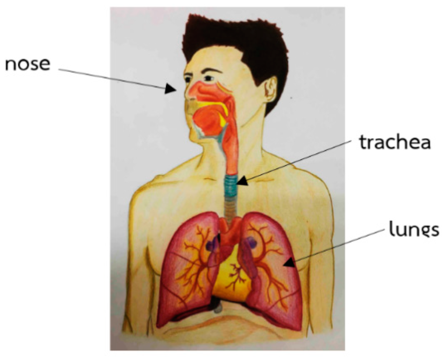
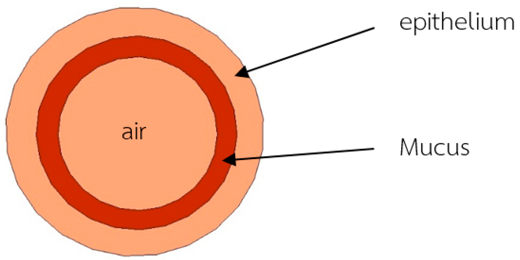
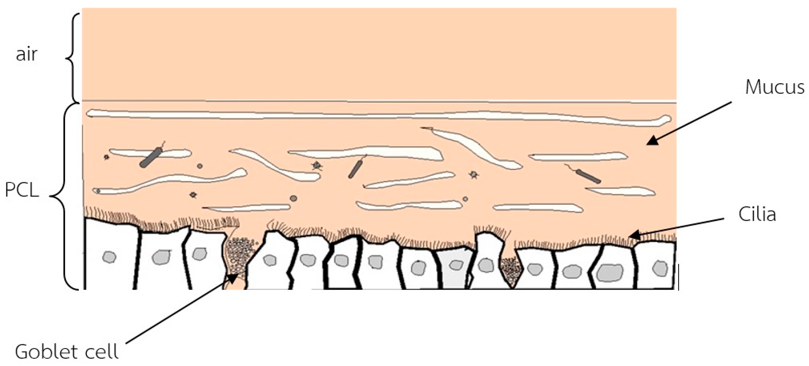
The human body contains numerous cilia, which are omnipresent inside and outside of the body. Cilia are hair-like organelles that provide locomotion to liquids throughout the body. This study focuses on cilia inside the body, particularly in the respiratory system. The human respiratory system is illustrated in Figure 1, with labeling of the nose, trachea, and lungs. We breathe in and out all the time, and as we inhale, some dust and pathogens will enter the body. However, the human body has a defense mechanism to protect against these foreign particles. In a closer look at the immune system, a diagram representing a cross-section of the trachea is displayed in Figure 2, and Figure 3 shows a close-up view of the trachea.
Figure 3 shows the platform of the innate immune system of the throat cells, which consists of three layers: The air layer, the mucus layer, and the periciliary layer (PCL). Cilia are found in the PCL layer. The function of the cilia is to filter out dust and other inhaled foreign particles. Cilia work as a part of the immune system, protecting the body against pathogens in the air. Goblet cells (vital component cells of the immune system) secrete mucus to trap the inhaled particles and cilia help to transport these particles out of the body by cilia-generated flow. To calculate the mucus velocity, the velocity of PCL fluid is measured to determine the bottom boundary of the mucus layer.
Numerical studies on the PCL and mucus layers have been carried out by several researchers. For example, Machemer [1] observed the ciliary system and found that frequency of peristomal cilia decreases with increasing viscosity, which leads to an increase of the average wavelength from 10.7 at 1 cP to 14.3 at 40 cP. Smith et al. [2] developed a new model for the nodal flow, utilizing the regularized stokeslet method. Fulford and Blake [3] studied a two-layer Newtonian fluid model for muco-ciliary transportation in the lung, and discovered that the viscosity of the upper mucous layer is much greater than the viscosity of the lower periciliary layer. Jayathilake et al. [4] developed a three-dimensional numerical model to simulate human pulmonary cilia motion in the PCL using the immersed boundary method combined with the projection method. Their numerical results indicated that the phase differences of cilia—in both stream-wise and span-wise directions—resulted in the maximum PCL velocity in the stream-wise direction.
Another approach on the study of the PCL and mucus layers is experimental study, which has been examined by a number of researchers. For example, Serafini and Michaelson [5] determined ciliary length and the percentage of ciliated cells from six mongrel dogs and ten humans. Matsui et al. [6] studied the movements of mucus and PCL liquid in airway surfaces, using conventional and confocal microscopy of fluorescent microspheres photoactivated fluorescent dyes and well-differentiated human tracheobronchial epithelial cell cultures that exhibited spontaneous, radial mucociliary transport. Their findings showed that the entire PCL liquid was transported at approximately the same rate as mucus, 39 ± 24.7 and 39.8 ± 4.2 µm/s. Moreover, they found that the removal of the mucus layer reduced PCL transport by >80%, 4.8 ± 0.6 µm/s, which is close to the value predicted by theoretical analyses of the ciliary beat cycle. Therefore, it has been suggested that the movement of PCL liquid depends on the transport of mucus.
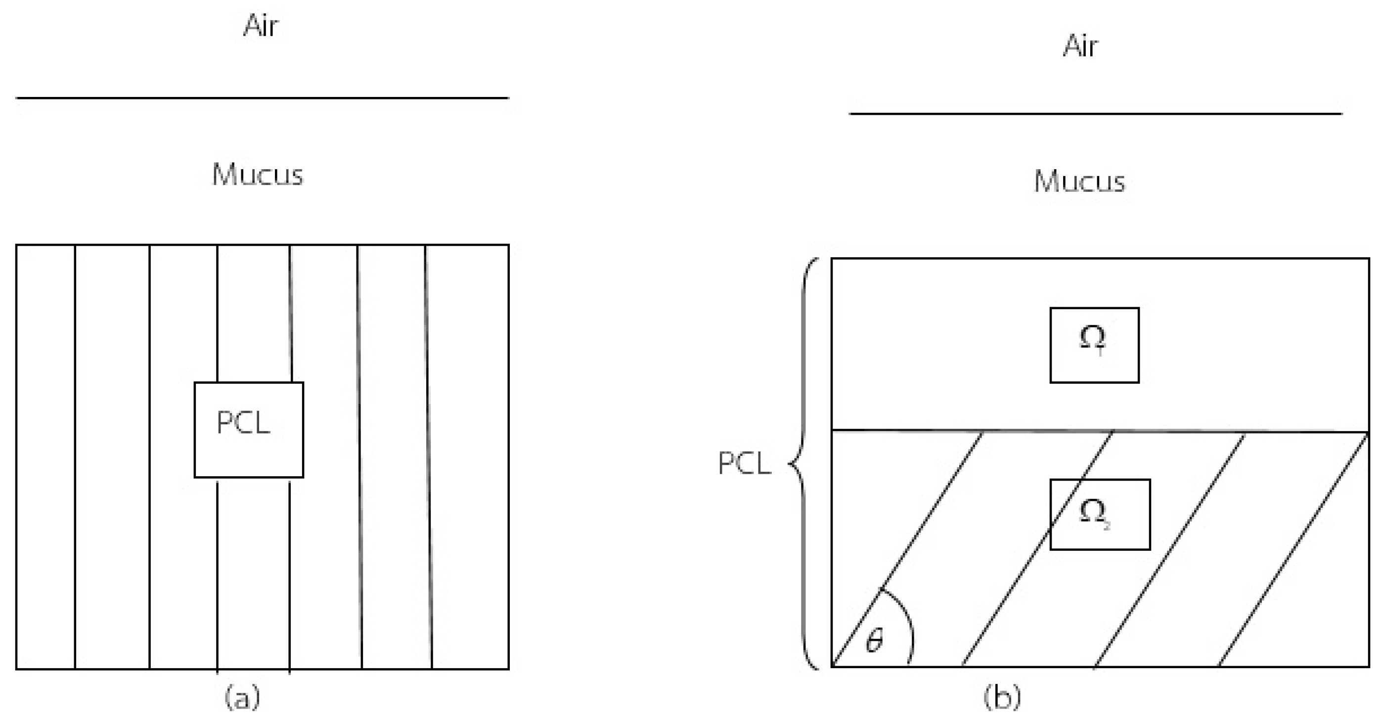
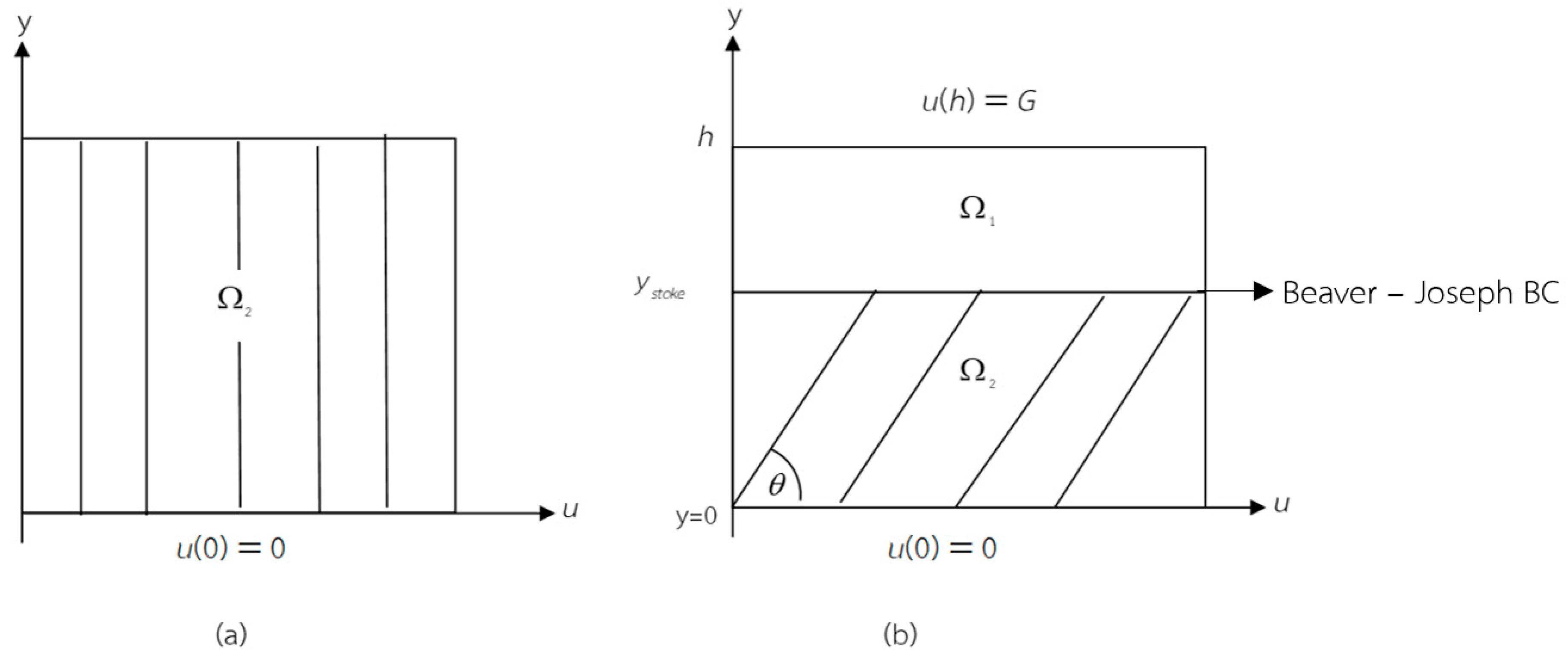
Although the study of PCL and mucus layers, both numerical and experimental studies, has been investigated extensively, these studies covered only movement, length, and direction of cilia; the research on velocity of cilia in the PCL layer is limited. In general, the asymptotic expansion method is used to examine the PCL fluid flow order to determine the velocity of PCL fluid. Cilia in the PCL layer are shown in Figure 4; cilia making a 90° angle with the horizontal plane are displayed in Figure 4a, while cilia at an angle of less than 90° are illustrated in Figure 4b. The domain is the PCL with an absence of cilia. The second domain, is the PCL containing cilia.
As the domain contains both liquid and solid phases, it is considered to be a porous medium. For the mathematical model used in the free fluid and the porous medium domains, some studies have used Navier-Stokes in the free fluid layer and Darcy in the porous medium [7], or Stokes equation in the free fluid layer and the Brinkman equation in the porous medium [8,9]. The Beavers-Joseph condition has been widely used in many numerical studies as well as to compare solutions, especially between a porous medium and a free fluid domain. For example, Francisco et al. [10] derived boundary conditions that complete the statement of a two-domain approach for a one-dimensional momentum transport in a system containing a porous medium and free fluid under a constant pressure gradient. These boundary conditions involve a jump in both the velocity and the viscous stress and are thus expressed in terms of jump coefficients.
In this paper, we use the Stokes equation in the free fluid region and the Brinkman equation in the porous medium in order to analytical study the Stoke–Brinkman equations. The asymptotic expansion method has been widely used in a number of studies [11,12,13]. Chandesris and Jamet [14] found the boundary condition at the interface between the porous medium and the free fluid based on the Poiseuille flow over a permeable block. The problem was solved using the matched asymptotic expansion method, therefore, both a heterogeneous transition zone and a homogeneous zone between the two homogeneous regions (porous medium and free fluid) were considered. The two homogeneous regions were described using volume averaged transport equation, with the assumption that this equation still holds in the heterogeneous transition zone by considering variable porosity and permeability.
However, to the authors’ knowledge, no study to date has used asymptotic expansion related to the velocity of the cilia in the model. The model used in the present study involves the velocity of solid helping to move the PCL fluid. In this study, we provide the velocity of the PCL fluid by using asymptotic expansion due to the movement of cilia where the Beaver–Joseph boundary condition is employed at the free fluid/porous medium interface.
In Section 2, we write n-dimensional Stokes–Brinkman equations in one dimension by using the indicial notation. The dimensionization of the governing equations is derived in Section 3. The solutions of the Stokes–Brinkman equations are computed with the asymptotic expansion method in Section 4. In Section 5, we determine the relation of the constants. We describe result and discussion in Section 6, and in Section 7 we draw our conclusions.
2. Mathematical Model and Boundary Conditions
In this section, we introduce our governing equations: the n-dimensional Stokes–Brinkman equations and the boundary conditions used in the PCL.
2.1. Stokes–Brinkman Equations
The n-dimensional Stokes–Brinkman equations were derived using an upscaling method, which is a method that helps to change the equations from a microscopic scale to a macroscopic scale. Then, we simplified the equations to one dimension by using an indicial notation. The macroscale Stokes–Brinkman equations [12] and the continuity equation [12] in n dimension are
respectively, where the function is a dynamic viscosity; is the inverse of the permeability tensor; is the porosity; and are the velocities of the liquid and solid phases, respectively; is the pressure; is the fluid density; is gravity; and is the material time derivative of the porosity with respect to the solid phase, . Equation (1) is the Brinkman equation. Without the first and fifth terms in the equation, it is a Stokes equation. Thus, in general, Equation (1) is called a Stokes–Brinkman equations. Applying the indicial notation to the Stokes–Brinkman equations we obtain
where the repeat index indicates the summation. Substituting Equation (4) into the last term of Equation (3), for the one-dimensional domain, we have
Note that . Simplifying Equation (5) yields
In this study, we assume that the solid velocity depends on only the direction; the fluid flow along the -axis; and the pressure depends on the direction. As a result, Equation (6) becomes
Equation (7) is a Brinkman equation, which is used in the domain containing cilia.
In region , we use a Stokes equation,
The continuity equation applied in this region is
For the free fluid region, we use a Stokes equation in domain . The equation is actually the Brinkman equation, without the permeability term.
Notice that we have two different and adjacent domains. Therefore, a boundary used at the interface is special. In this work we applied the Beavers–Joseph boundary condition at the interface between the free fluid region and the porous medium domain.
2.2. Boundary Conditions
No free fluid exists in the PCL when the cilia are perpendicular to the horizontal plane. Figure 5a shows that the PCL has only domain . Figure 5b shows our domains and ; the boundary condition between and is at at the tips of the cilia. Note that depends on the angle . We used 3 boundary conditions in this study at , at and Beavers–Joseph boundary condition at .
Let . We now have the system of equations with the unknown and boundary conditions;
where is a dimensionless parameter of the order of one; is porosity of the porous medium; is length of porous medium; and is a function depending on and the angle .
3. Dimensionless Stokes–Brinkman Equations
In this section, we normalize the Stokes–Brinkman equations by introducing the following new variables.
where is the characteristic length; is volumetric average velocity in the porous medium; is characteristic permeability; and is characteristic gravity.
3.1. Dimensionless of Brinkman Equation
We normalize the Brinkman equation, of Equation (7) by substituting Equation (13) for Equation (7). We then have
Equation (14) can be rewritten as
where are constants and
3.2. Dimensionless Stokes Equation
We normalize the Stokes Equation (8) by substituting Equation (13) for Equation (8). We then obtain
Equation (17) can be rewritten as
where and are the constants defined in Equation (16).
3.3. Dimensionless Boundary Conditions
In this section we normalize the boundary conditions at the free fluid/porous medium interface used in our domain.
Substituting Equation (13) for Equation (12) we have
Next, we normalize the bottom and top boundary conditions by substituting Equation (13) for Equation (10) and Equation (11), giving us
respectively.
We have now normalized the Stokes–Brinkman equations and the boundary conditions. Consequently, the system of equations used in the next sections and the boundary conditions are
4. Asymptotic Expansion Method of the Stokes–Brinkman Equations
As mentioned in Section 2, we have two different domains where the domain , is the region where and the region is the layer where . In this section, we find the analytical solution of the governing equations with the asymptotic expansion. Section 4.1 shows the result of the Brinkman equation and Section 4.2 shows the result of the Stokes equation.
4.1. Asymptotic Expansion Method of the Brinkman Equation
Using the method of asymptotic expansion, we assume that
In the case , we substitute Equation (27) for Equation (22), giving us
Considering the zeroth-order of ; we obtain
Since , the velocity of cilia, is a known source term in this work, we assume that it is a linear function. That is
where and are constants. Thus, Equation (29) becomes
First, we find the general solution of the homogeneous Equation (30). Solving the homogeneous part of the ordinary differential equation
We obtain the general solution . To find the particular solution of Equation (30), we use the method of undetermined coefficients. Therefore, the solution of the differential equation is
Let
all of which are constants. Therefore Equation (32) can be rewritten as
Applying Equation (24) to Equation (34), we have
which yields
We now have the solution of the Brinkman equation.
4.2. Asymptotic Expansion Method of Stokes Equation
Similar to the previous section, we calculate the velocity of the PCL fluid in domain using the asymptotic expansion method with the Stokes Equation (23). We assume that
In the case , we substitute Equation (37) for Equation (23). Therefore
Considering the zeroth-order term of , , we obtain
As we assume that is a constant, by integrating Equation (39) twice, we have
Applying the boundary condition (25) to Equation (40), we obtain
We can find the solutions at and , yet the constants and of the Stokes–Brinkman equation are unknown.
5. The Relation between the Constants
In this section, we determine the relation of the constants and with Beavers–Joseph boundary condition. Substituting Equation (36) and Equation (41) for Equation (26), we obtain
where (on the right-hand side of Equation (42)) can be obtained from the PCL velocity in , or both. However, the velocity is a slip velocity [13,14]. Therefore, in this work, we consider the case that .
Substituting Equation (41) for the right-hand side of Equation (42) and simplifying, we have
We now have the relation between the constants and . Inserting Equation (42) into Equation (41), we have the solution of the Stokes equation depending on . That is
We now obtain the general solution of the Stokes–Brinkman equations, depending only the constant with the asymptotic expansion method, in which the Beavers–Joseph condition is employed at the free fluid/ porous medium interface.
6. Results and Discussion
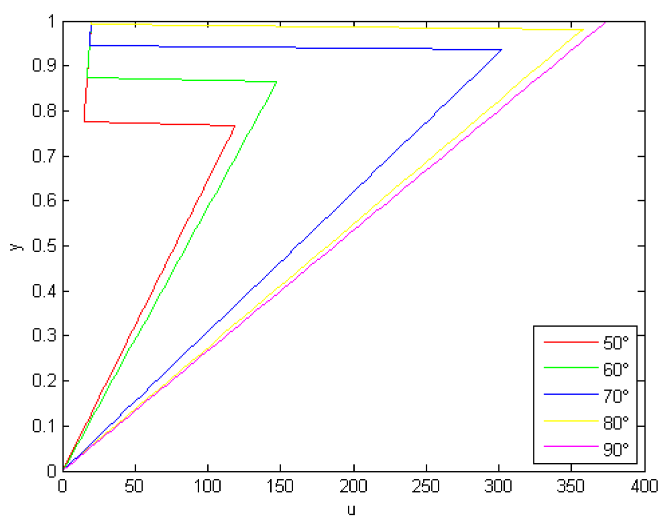
The solutions of Stokes–Brinkman equations, Equation (36) and Equation (44), calculated in Section 4 and Section 5 are plotted on a graph and discussed in this section. To plot the graph, we assume that the graphs between the cilia and the horizontal plane are where the cilia have the highest velocity at during the forward stroke and stop beating at . So, at we do not need to calculate the velocity of the PCL. The variables used in Equation (44) are given in Table 1 and Table 2. The values of and are obtained from [4], and is the velocities of the solid, cilia, where the maximum velocity of motile cilia value is assumed at in descending order of degree, terminating at , is the cilium height, is one cycle of ciliary beat, and and were obtained from [2]. We assume that the rate of pressure changes equals 1. The boundary condition at the top of the free fluid domain equals 1. The variable in Equation (44) equals 0 because in this study we aim to verify if the solid velocities applied to the equation are valid, the solutions correlate with the variable velocity employed, where the maximum velocity is assumed at and decreases with decreasing angles.
These solutions are the velocity of PCL fluid in the layer containing cilia with different angle respectively. It can be noted that the velocity decrease with decreasing angles and bends sharply at the seam of the porous medium and the free fluid region. The asymptotic solution of the Stoke–Brinkman Equation (44) is shown in Figure 6 (the code is given in Appendix here).
The asymptotic expansion method is the tool for finding analytical approximate solutions to complicated practical problems, for example, the problem in ordinary differential equations in terms of regular perturbation and singular perturbation. We construct different asymptotic solutions inside and outside the region of rapid change and match them together to determine a global solution. Other methods used for finding exact and approximate solutions for linear and nonlinear partial differential equations is the homotopy perturbation method which is only a special case of the homotopy analysis method. The basic ideas of the homotopy perturbation method is a coupling of the traditional perturbation method and homotopy in topology deforms continuously the problem in hand to a simple one which can be easily solved. The advantage of this method is that it can be applied to various nonlinear problems, and the disadvantage is that we should suitably choose an initial guess, or infinite iterations are required [15]. The asymptotic expansion method and the homotopy perturbation method are principally based on a Taylor series with respect to an embedding parameter.
Another method used to describe the samples with porous media, is the fractal derivative model. This method is developed from fractal calculus for calculating the solution of problem phenomena in porous media or hierarchical structures [16]. For instance, in a study by Wang, Shi, He, and Li [17], to find an optimal hair length of a polar bear for thermal protection, which helps maintain a normal body temperature, by using a fractal derivative model of one-dimensional heat conduction along the hair. The basic ideas of the fractal calculus begin from Fourier’s law of thermal conduction, which can be expressed as where is the heat flux, is the material’s conductivity, and is the temperature gradient, but the asymptotic expansion method is adopted to determine the velocity of ciliary motion that moves foreign particles out of the body.
While the asymptotic expansion method can be used to study the interface between the porous media region and the free fluid region, the homotopy perturbation method and the fractal derivative model are only adopted for the porous media domain. These three approaches are the tools for finding analytical approximate solutions to the problem in ordinary differential equations or partial differential equations. Another difference is that the asymptotic expansion method can be applied to solve linear ordinary differential equations and perturbation equations. On the other hand, the homotopy perturbation method and the fractal derivative model are used to derive the solutions to nonlinear ordinary differential equations or partial differential equations.
7. Conclusions
In this article, we studied the fluid flow in the periciliary layer (PCL) of the respiratory tract using the of asymptotic expansion method to determine the velocity of PCL fluid. The PCL is divided into two domains: the free fluid and the porous medium domains. The free fluid domain is the upper layer of the PCL from cilia are absent. The porous medium domain is the lower layer of PCL and contains cilia. The Stokes equation is employed in the free fluid domain and the Brinkman equation is applied in the porous medium. The Beavers–Joseph boundary condition is employed at the interface between the porous medium and the free fluid region. We assume that the velocity of the PCL fluid at the bottom of the porous medium domain (at ) is zero and the velocity of the PCL fluid in the porous medium depends on angle . The boundary condition at the top of the free fluid domain is assumed to be a function of , where depends on and the angle . The explicit formula of velocity of PCL fluid is obtained by applying asymptotic expansion to the Stokes–Brinkman equations.
Author Contributions
Conceptualization, S.P. and K.W.; methodology, S.P.; software, S.P.; validation, K.W. and S.P.; formal analysis, S.P.; investigation, S.P.; resources, S.P.; data curation, K.W.; writing—original draft preparation, S.P.; writing—review and editing, K.W.; visualization, S.P.; supervision, K.W.; project administration, K.W.; funding acquisition, S.P.
Funding
This research received no external funding.
Acknowledgments
The authors would to thank Rachada Pongprairat and Krongkaew Mighanetara for advice and support.
Conflicts of Interest
The authors declare no conflict of interest.
Nomenclature
| Variable | Meaning | Unit |
| a dynamic viscosity | ||
| the inverse of the permeability tensor | ||
| a porosity | ||
| the velocities of the liquid | ||
| the velocities of the solid | ||
| pressure | ||
| the material time derivative of the porosity with respect to the solid phase | ||
| the characteristic length | ||
| a volumetric average velocity in a porous medium | ||
| characteristic permeability | ||
| characteristic gravity | ||
| gravity |
Appendix A
%==========================================================================
   %================= This Program for Compute the Solutions =================
   %==========================================================================
   clear all;
clc;
format long;
%% Set Value
yStoke = [0.7672 0.8638 0.9353 0.9818 1.0];
K11 = [0.0012 0.0015 0.0016 0.0017 0.0018];
Eps = [0.6716 0.7099 0.7331 0.7439 0.7487];
c = [0 0.0023; 0 0.0024;0 0.0044; 0 0.0049; 0 0.0050];
c = c*10^(5);
h = 7.5;
Rho = 992.2*10^(-15);
Mu = 3*power(10,-6);
g = 9.81*10^(6);
u0 = 0.05;
Beta = 1;
h = 7.5;
Kp = K11;
vPlus = 100;
dPplus = 10;
w1 = 0;
G = 1;
gram = [0 -0.05 0.06 0.16 -0.3];
% phiP = 1-6.*gram;
phiP = Eps;
angle = 50:10:90;
% Left and Right Boundary of Part 1 and 2
% Step Size of Y
noY = 50;
yy1 = [linspace(0,yStoke(1),noY); linspace(0,yStoke(2),noY);...
          linspace(0,yStoke(3),noY); linspace(0,yStoke(4),noY);...
		linspace(0,yStoke(5),noY)];
y1 = linspace(0,yStoke(5),noY+noY);
yy2 = [linspace(yStoke(1)+0.01,1,noY); linspace(yStoke(2)+0.01,1,noY);...
        linspace(yStoke(3)+0.01,1,noY); linspace(yStoke(4)+0.01,1,noY)];
y = [yy1(1:4,:) yy2; y1];
nData = length(yStoke);
% Color and Style Orders of line in each figure
Col = {’r’; ’g’; ’b’; ’y’; ’m’};
Style = {’-’; ’-’; ’-’; ’-’; ’-’};
% Parameter of part 1
M1 = 1./Eps;
M2 = (h^(2))./(K11);
M3 = ((h^(2))*Rho*g)/(Mu*u0);
J1 = sqrt(M2./(2*M1));
J2 = dPplus./M2;
J3 = (h^(2).*Eps)./(M2.*K11);
J4 = M3./M2;
%% Define and Compute the solutions
for i = 1 : nData
    % Part 1
    t1 = J2(i)-J4(i)-(J3(i)*c(i,1));
    t2 = J3(i)*c(i,2);
    % Computation of part 1
    j = 1;
    if i ~= nData
	for y1p = 1 : noY
            uu1(i,j) = w1*exp(J1(i)*yy1(i,y1p))-w1*exp(-J1(i)*yy1(i,y1p))...
                  +t1*exp(-J1(i)*yy1(i,y1p))+t2*yy1(i,y1p)-t1;
            j = j+1;
        end
    else
        for y1p = 1 : noY
            uu1(i,j) = w1*exp(J1(i)*yy1(i,y1p))-w1*exp(-J1(i)*yy1(i,y1p))...
                  +t1*exp(-J1(i)*yy1(i,y1p))+t2*yy1(i,y1p)-t1;
            j = j+1;
        end
        j = 1;
        for y1p = 1 : 2*noY
            u1(1,j) = w1*exp(J1(i)*y1(1,y1p))-w1*exp(-J1(i)*y1(1,y1p))...
                  +t1*exp(-J1(i)*y1(1,y1p))+t2*y1(1,y1p)-t1;
            j = j+1;
        end
    end
    % Part 2
    f1 = exp(J1(i)*(yStoke (i)/h));
    f2 = exp(-J1(i)*(yStoke (i)/h));
    f3 = yStoke (i)/h;
    f4 = G/u0;
    f5 = ((1/2)*J2(i)-(1/2)*J4(i));
    f6 = 1/phiP(i);
    f7 = (h*Beta)/sqrt(Kp(i));
    if i ~= nData
        j = 1;
        % Computation of part 2 : Case 3 eq 4.23
        for y2p = 1 : noY
            s4(i,j) = (1/(1-f7*f3+f7))*((w1*(f6*J1(i)*f1+f6*J1(i)*f2))...
                       +((f7*f5*f3^2)/2)+f7*f4-((f7*f5)/2)...
                     -f5*f3-(f6*J1(i)*t1*f2)+(f6*J3(i)*c(i,2)));
            uu4(i,j) = ((f5/2)*(yy2(i,y2p))^2)+(s4(i,j)*yy2(i,y2p))...
                +f4-(f5/2)-s4(i,j);
            j = j+1;
        end
        nPlot2{i,1} = [num2str((10*i)+40),’\circ’];
    end
    nPlot1{i,1} = [num2str((10*i)+40),’\circ’];
end
UU2 = cat(2,uu1(1:4,:),uu2(1:4,:));
UU3 = cat(2,uu1(1:4,:),uu3(1:4,:));
UU4 = cat(2,uu1(1:4,:),uu4(1:4,:));
U2 = cat(1,UU2,u1);
U3 = cat(1,UU3,u1);
U4 = cat(1,UU4,u1);
%% Plot Graph
% Plot Graph of each part
% part 1
figure();
plot(uu1(1,:),yy1(1,:),’r’,uu1(2,:),yy1(2,:),’g’,uu1(3,:),yy1(3,:),’b’...
      ,uu1(4,:),yy1(4,:),’y’,uu1(5,:),yy1(5,:),’m’);
  % case 3
   figure();
  plot(uu4(1,:),yy2(1,:),’r’,uu4(2,:),yy2(2,:),’g’,uu4(3,:),yy2(3,:),’b’...
        ,uu4(4,:),yy2(4,:),’y’);
  xlabel(’u’)
   ylabel(’y’)
   title(’The solution of u and y when y^{+} > y_{stoke} : case 3’)
   legend(nPlot2,-1);
  % Plot Graph of all degree
   l = length(y);
   % case 3
   figure();
  plot(U4(1,:),y(1,:),’r’,U4(2,:),y(2,:),’g’,U4(3,:),y(3,:),’b’...
        ,U4(4,:),y(4,:),’y’,U4(5,:),y(5,:),’m’)
   xlabel(’u’)
   ylabel(’y’)
   % title([’The relation between u and y when y^{+} < y_ {stoke} ’...
        %     ’and y^{+} > y_{stoke} : case 3’])
   legend(nPlot1,4);
  saveas(gcf,’CompareSolStokeCase3.fig’)
References
- Machemer, H. Ciliary activity and the origin of metachrony in paramecium: Effects of increasd viscocity. J. Exp. Biol. 1972, 57, 239–259. [Google Scholar] [PubMed]
- Smith, D.J.; Smith, A.A.; Blake, J.R. Mathematical embryology: The fluid mechanics of nodal cilia. J. Eng. Math. 2011, 70, 255–279. [Google Scholar] [CrossRef]
- Fulford, G.R.; Blake, J.R. Muco–ciliary transport in the lung. J. Thero. Biol. 1986, 121, 381–402. [Google Scholar] [CrossRef]
- Jayathilake, P.G.; Tan, Z.; Le, D.V.; Lee, H.P.; Khoo, B.C. Three-dimensional numerical simulations of human pulmonary cilia in the periciliary liquid layer by the immersed boundary method. Comput. Fluids Sciencedirect. 2012, 67, 130–137. [Google Scholar] [CrossRef]
- Serafini, S.M.; Michaelson, E.D. Length and distribution of cilia in human and canine airways. Bull. Eur. Pysiopathol. Respir. 1977, 13, 551–559. [Google Scholar]
- Matsui, H.; Randell, S.H.; Peretti, S.W.; Davis, C.W.; Boucher, R.C. Coordinated clearance of pericilary liquid and mucus from airway surfaces. J. Clin. Investig. 1998, 102, 1125–1131. [Google Scholar] [CrossRef] [PubMed]
- Neale, G.; Nader, W. Practical significance of Brinkman’s extension of Darcy’slaw: Coupled parallel flows within a channel and a bounding porous medium. Can. J. Chem. Eng. 1974, 52, 475–478. [Google Scholar] [CrossRef]
- Ochoa, J.A.; Whitaker, S. Momentum transfer at the boundary between a porous medium and a homogeneous fluid—I. Theoretical development. Int. J. Heat Mass Transf. 1995, 38, 2635–2646. [Google Scholar] [CrossRef]
- Ochoa, J.A.; Whitaker, S. Momentum transfer at the boundary between a porous medium and a homogeneous fluid—II. Comparison with experiment. Int. J. Heat Mass Transfer 1995, 38, 2647–2655. [Google Scholar] [CrossRef]
- Valdes-Parada, F.J.; Aguilar-Madera, C.G.; Ochoa-Tapia, J.A.; Goyeau, B. Velocity and stress jump conditions between a porous medium and a fluid. Adv. Water Resour. 2013, 62, 327–339. [Google Scholar] [CrossRef]
- Chamsri, K. Formulation of a well-posed Stoke-Brinkman Problem with a Permeability Tensor. J. Math. 2015, 1, 1–7. [Google Scholar]
- Wuttanachamsri, K.; Schreyer, L. Effects of the Cilia movement on fluid Velocity for fixed Domain. submitted.
- Sears, P.R.; Thomson, K.; Knowles, M.R.; Davis, C.W. Human Airway Ciliary Dynamics. Am. J. Physiol. Lung Cell. Mol. Physiol. 2012, 704, L170–L183. [Google Scholar] [CrossRef] [PubMed]
- Chandesris, M.; Jamet, D. Boundary conditions at a planar fluid-porous interface for a Poiseuille flow. Int. J. Heat Mass Transf. 2006, 49, 2137–2150. [Google Scholar] [CrossRef]
- Homotopy Perturbation Method. Available online: www.shodhganga.inflibnet.ac.in/bitstream/10603/37622/9/09_chapter%202.pdf (accessed on 15 May 2019).
- He, J.-H. Fractal calculus and its geometrical explanation. Results Phys. 2018, 10, 272–276. [Google Scholar] [CrossRef]
- Fractal Calculus and Its Application to Explanation of Biomechanism of Polar Bear Hairs. Available online: www.Worldsciencetific (accessed on 3 May 2019).
Figure 1.
The human respiratory system.

Figure 2.
A cross-section of the trachea.

Figure 3.
Platform of the innate immune system.

Figure 4.
Cartoon picture of cilia (a) cilia are perpendicular to the horizontal plane; (b) cilia make angle with the horizontal plane.
Figure 4.
Cartoon picture of cilia (a) cilia are perpendicular to the horizontal plane; (b) cilia make angle with the horizontal plane.

Figure 5.
Cilia making the angle with the horizontal plane. (a) cilia are perpendicular to the horizontal plane; (b) cilia make angle with the horizontal plane.
Figure 5.
Cilia making the angle with the horizontal plane. (a) cilia are perpendicular to the horizontal plane; (b) cilia make angle with the horizontal plane.

Figure 6.
The asymptotic solution of the Stoke–Brinkman equations.


Table 1.
Variable of the experimental data in the solution of the Stoke–Brinkman equations.
| Variable | Value | Unit |
|---|---|---|
| h | 7.5 | |
| 1.00 | ||
| 1 | ||
| 1 | ||
| 1 | ||
| 0 | ||
| 1 |
Table 2.
Values of variables used in Equation (44) used to plot Figure for each angle .
| Variable | |||||
|---|---|---|---|---|---|
| 0.7672 | 0.8638 | 0.9353 | 0.9818 | 1.0000 | |
| 0.0012 | 0.0015 | 0.0016 | 0.0017 | 0.0018 | |
| 0.6717 | 0.7099 | 0.7331 | 0.7439 | 0.7487 | |
| 0.0023 | 0.0024 | 0.0044 | 0.0049 | 0.0050 |
© 2019 by the authors. Licensee MDPI, Basel, Switzerland. This article is an open access article distributed under the terms and conditions of the Creative Commons Attribution (CC BY) license (http://creativecommons.org/licenses/by/4.0/).
Share and Cite
MDPI and ACS Style
Poopra, S.; Wuttanachamsri, K. The Velocity of PCL Fluid in Human Lungs with Beaver and Joseph Boundary Condition by Using Asymptotic Expansion Method. Mathematics 2019, 7, 567. https://0-doi-org.brum.beds.ac.uk/10.3390/math7060567
AMA Style
Poopra S, Wuttanachamsri K. The Velocity of PCL Fluid in Human Lungs with Beaver and Joseph Boundary Condition by Using Asymptotic Expansion Method. Mathematics. 2019; 7(6):567. https://0-doi-org.brum.beds.ac.uk/10.3390/math7060567
Chicago/Turabian StylePoopra, Sudaporn, and Kanognudge Wuttanachamsri. 2019. "The Velocity of PCL Fluid in Human Lungs with Beaver and Joseph Boundary Condition by Using Asymptotic Expansion Method" Mathematics 7, no. 6: 567. https://0-doi-org.brum.beds.ac.uk/10.3390/math7060567
Note that from the first issue of 2016, this journal uses article numbers instead of page numbers. See further details here.