n0-Order Weighted Pseudo Δ-Almost Automorphic Functions and Abstract Dynamic Equations


1
Department of Mathematics, Yunnan University, Kunming 650091, China
2
Distinguished University Professor of Mathematics, Florida Institute of Technology, 150 West University Boulevard, Melbourne, FL 32901, USA
3
Department of Mathematics, Texas A&M University-Kingsville, Kingsville, TX 78363-8202, USA
4
School of Mathematics, Statistics and Applied Mathematics, National University of Ireland, Galway, Ireland
5
Department of Mathematics, Morgan State University, 1700 E. Cold Spring Lane, Baltimore, MD 21251, USA
*
Author to whom correspondence should be addressed.
Mathematics 2019, 7(9), 775; https://0-doi-org.brum.beds.ac.uk/10.3390/math7090775
Submission received: 17 July 2019
/
Revised: 17 August 2019
/
Accepted: 19 August 2019
/
Published: 22 August 2019
Abstract
:In this paper, we introduce the concept of a -order weighted pseudo -almost automorphic function under the matched space for time scales and we present some properties. The results are valid for q-difference dynamic equations among others. Moreover, we obtain some sufficient conditions for the existence of weighted pseudo -almost automorphic mild solutions to a class of semilinear dynamic equations under the matched space. Finally, we end the paper with a further discussion and some open problems of this topic.
Keywords:
time scales; seighted pseudo Δ-almost automorphic functions; abstract dynamic equations; mild solutionsMSC:
26E70; 33E30; 34N05; 43A601. Introduction
In 1962, Bochner introduced the concept of an almost automorphic function on the real numbers (see [1]) and such functions and applications were studied in [2,3,4,5]. In the literature [6,7,8,9,10,11], existence and uniqueness of pseudo almost automorphic solutions to semilinear abstract differential equations were studied. In [12], the authors proposed a concept of weighted pseudo almost automorphic functions (WPAA) and completeness and a composition theorem of the function space formed by WPAA were obtained (this generalizes weighted pseudo almost periodic functions [13,14,15,16]).
Almost periodic and almost automorphic problems of dynamic equations on time scales were studied in [17,18,19,20,21,22,23,24,25]. In 1988, Hilger [26] (see also the books [27,28]) initiated the theory of time scales. An arbitrary closed nonempty subset of the reals is called a time scale and it covers the theories of classical differential and of difference equations (see [29,30]). Based on the translation regularity of periodic time scales, the definition of almost automorphic functions on regular periodic time scales was successfully proposed because of the nice translation-closedness for all periodic time scales. However, for the translation irregularity of some basic time scales such as or (which is widely applied to quantum or quantum-like theory) and other types of time scales such as and the space of the harmonic numbers, it is very difficult to introduce almost automorphic functions (note it is of interest to study almost automorphic dynamic behavior of solutions to quantum-like dynamic equations including q-difference dynamic equations and others). In the literature [31], the authors introduced and studied a new type of almost periodic functions and stochastic process in which the almost periodic functions and dynamic equations on quantum-like time scales was investigated for the first time.
In this paper, by employing the concept of matched spaces theory, the strict shift-closedness of time scales will be guaranteed under non-translational shift (see [32]), the concepts of -almost automorphic functions and -order weighted pseudo -almost automorphic functions are introduced and their basic properties are obtained. Using this, we establish some sufficient conditions to obtain the existence of weighted pseudo -almost automorphic mild solutions to a class of semilinear dynamic equations involving quantum-like dynamic equations like q-difference dynamic equations and others.
The organization of this paper is as follows: in Section 2, we introduce the concept of -almost automorphic functions and -order weighted pseudo -almost automorphic functions under the matched space of time scales, and some properties are presented. In Section 3, the existence of weighted pseudo -almost automorphic mild solutions is investigated for a type of abstract semilinear dynamic equations. In Section 4 and Section 5, an example is provided and a further discussion is conducted with some interesting open problems of this topic.
2. N0-Order Weighted Pseudo Δ-Almost Automorphic Functions
In this part, first, we will recall some basic knowledge of matched spaces for time scales. For more details of dynamic equations on time scales and matched spaces, the reader may consult [26,27,28,32,33,34].
Definition 1
([32]). Let be a subset of together with an operation and the pair be an Abelian group, and be increasing with respect to its second argument, i.e., and satisfy the following conditions:
- (1)
- is closed with respect to the operation , i.e., for any , we have .
- (2)
- There exists an identity element such that for all .
- (3)
- For all , and .
- (4)
- For each , there exists an element such that , where is the identity element in .
- (5)
- If , then .
A subset S of is called relatively dense with respect to the pair if there exists a number such that (or ) for all . The number is called the inclusion length with respect to the group .
From Definition 1, for example, let . Then, and
We can obtain the following definition.
Definition 2
([32]). A subset S of is called relatively dense with respect to the pair if there exists a number such that for all and for all . The number L is called the inclusion length with respect to the group .
Definition 3
([32]). Let and be time scales, where , and is a sub-timescale of for each . If is the largest open subset of the time scale , i.e., , where denote the closure of the set A, and is an Abelian group, are countable index sets; then, we say is an adjoint set of if there exists a bijective mapping:
i.e., . Now, F is called the adjoint mapping between and .
Remark 1.
A subset K of a time scale is said to be a sub-timescale of if and only if is a time scale.
Remark 2.
Note that the largest open subset of a time scale (i.e., the topological interior of a time scale) is unique. For example, let ; then, ; let ; then, ; let ; then, . For other classical cases, for instance, let ; then, ; let (); then, , etc.
Definition 4
([32]). Let the pair be an Abelian group and be the largest open subsets of the time scales and , respectively. Furthermore, let be the adjoint set of and F the adjoint mapping between and . The operator satisfies the following properties:
- (P1)
- (Monotonicity) The function δ is strictly increasing with respect to all its arguments, i.e., ifthen, implies ; if with , then .
- (P2)
- (Existence of inverse elements) The operator δ has the inverse operator and , where is the inverse element of τ.
- (P3)
- (Existence of identity element) and for any , where is the identity element in .
- (P4)
- (Bridge condition) For any and , .
Then, the operator associated with is said to be a shift operator on the set . The variable in δ is called the shift size. The value in indicates s units shift of the term . The set is the domain of the shift operator δ.
Now, we present the concept of matched spaces for time scales.
Definition 5
([32]). Let the pair be an Abelian group, and be the largest open subsets of the time scales and , respectively. Furthermore, let be an adjoint set of and F the adjoint mapping between and . If there exists the shift operator δ satisfying Definition 4, then we say the group is a matched space for the time scale .
Definition 6
In the following, we always assume that the group is a regular matched space of which is a periodic time scale in the sense of Definition 6. For concise notation, we use the symbols and . For convenience, we denote and is a Banach space.
For a matched space , we denote the sub-timescale which the argument t belongs to, and clearly, , where is an index set satisfying .
Remark 3.
By Definition 6, we will demonstrate the following time scales are periodic under matched spaces:
- (i)
- is periodic since , where and .
- (ii)
- is periodic since , where and .
- (iii)
- is periodic since . In fact,where , and , . Note that .
Remark 4.
In Remark 3 , from the property of the operation δ (note that δ is discontinuous at ), we can obtain the right shift closedness of and the left shift closedness of , respectively.
Theorem 1.
If is a periodic time scale under a matched space in the sense of Definition 6, then , where .
Proof.
For any , we have . Moreover, for any , there exists some and such that . This completes the proof. □
Let , we introduce a function ,
Let
and denote a function space which has the property that ; if , then for all and , where denotes a bounded function space from to .
Remark 5.
From definition of , if is Δ-differentiable for all , then .
Remark 6.
If is a time scale which satisfies Definition 6 and , then it follows that . In fact, from Definition 6, we can obtain that and it implies that .
Remark 7.
Let . Then, we can get . Hence,
and, for ,
Note that is continuous in if and only if , which implies that, for any , is not continuous at , i.e., is not Δ-differentiable at for . Moreover, has oriented shift closedness in parts by starting with . In this example, the part has closedness during right shift and the other part has closedness during left shift.
Definition 7
([32]). If the adjoint mapping is continuous and satisfies
- (1)
- for any , holds;
- (2)
- if and , then ,
we say is a regular matched space for the time scale .
Lemma 1.
If the time scale is periodic in the sense of Definition 6 and is a regular matched space, then for any fixed point , there exists a suitable adjoint mapping such that .
Proof.
Since the time scale is periodic in the sense of Definition 6, then is also the identity element in .
From Definition 6, there exists an inverse element such that , so there exists a suitable constant such that . In fact, from condition of Definition 7, let , we have . Thus, we have . This completes the proof. □
Remark 8.
From condition in Definition 7, if for a fixed , then it follows that for and for .
Next, we will introduce the concepts of -almost automorphic functions and -order Δ-almost automorphic functions (i.e., -almost automorphic functions).
Definition 8
(δ-almost automorphic functions).
- (i)
- Let be a bounded continuous function. f is said to be δ-almost automorphic under the matched space if for every sequence of real numbers one can extract a subsequence such that:is well defined for each and a sequence that is dependent on such thatfor each Denote by the set of all such functions.
- (ii)
- A continuous function is said to be δ-almost automorphic if is δ-almost automorphic in uniformly for all where B is any bounded subset of Denote by the set of all such functions.
If there exists inverse element in for each , then and Definition 8 can be written into the following form by taking .
Definition 9.
- (i)
- Let be a bounded continuous function and is Δ-differentiable. f is said to be δ-almost automorphic under the matched space if for every sequence of real numbers one can extract a subsequence such that:is well defined for each andfor each Denote by the set of all such functions.
- (ii)
- A continuous function is said to be δ-almost automorphic if is δ-almost automorphic in uniformly for all where B is any bounded subset of Denote by the set of all such functions.
As an extension of Definition 8, we can introduce the following concept.
Definition 10
(-almost automorphic functions).
- (i)
- Let be a bounded continuous function. f is said to be-order Δ-almost automorphic (-almost automorphic) under the matched space if there exists some such that, for every sequence of real numbers we can extract a subsequence such that:is well defined for each and a sequence that is dependent on such thatfor each , whereDenote by the set of all such functions.
- (ii)
- A continuous function is said to be -order -almost automorphic if is -almost automorphic in uniformly for all where B is any bounded subset of Denote by the set of all such functions.
In fact, if there exists inverse element in for each , then Definition 10 can also be written into the following form by taking .
Definition 11.
- (i)
- Let be a bounded continuous function and is Δ-differentiable. f is said to be -order Δ-almost automorphic (-almost automorphic) under the matched space if there exists some such that for every sequence of real numbers we can extract a subsequence such that:is well defined for each andfor each , whereDenote by the set of all such functions.
- (ii)
- A continuous function is said to be -order -almost automorphic if is -almost automorphic in uniformly for all where B is any bounded subset of Denote by the set of all such functions.
Remark 9.
Note that the condition “ is Δ-differentiable” from Definitions 9 and 11, which implies according to Remark 5.
Remark 10.
Let , so
Then, f is said to be a standard -almost automorphic function.
Remark 11.
In Definition 10, let and ; if or , then and the following classical concepts can be obtained.
Definition 12
(Case I. , [2]).
- (i)
- Let be a bounded continuous function. f is said to be almost automorphic if for every sequence of real numbers , one can extract a subsequence such that:is well defined for each andfor each
- (ii)
- A continuous function is said to be almost automorphic if is almost automorphic in uniformly for all where B is any bounded subset of
Definition 13
(Case II. , [2]).
- (i)
- Let be a bounded continuous function. f is said to be almost automorphic if for every sequence of real numbers , one can extract a subsequence such that:is well defined for each andfor each
- (ii)
- A continuous function is said to be almost automorphic if is almost automorphic in uniformly for all where B is any bounded subset of
Now, we construct an -almost automorphic function through through the following steps.
Example 1.
Consider and , we introduce the operators as follows:
then it follows that is a matched space of the time scale , where for all , . Note that , where .
Step 1. Periodic function construction. Since is periodic under the matched space , we construct the following function
under a matched space , then it follows that the function is periodic with the period . In fact,
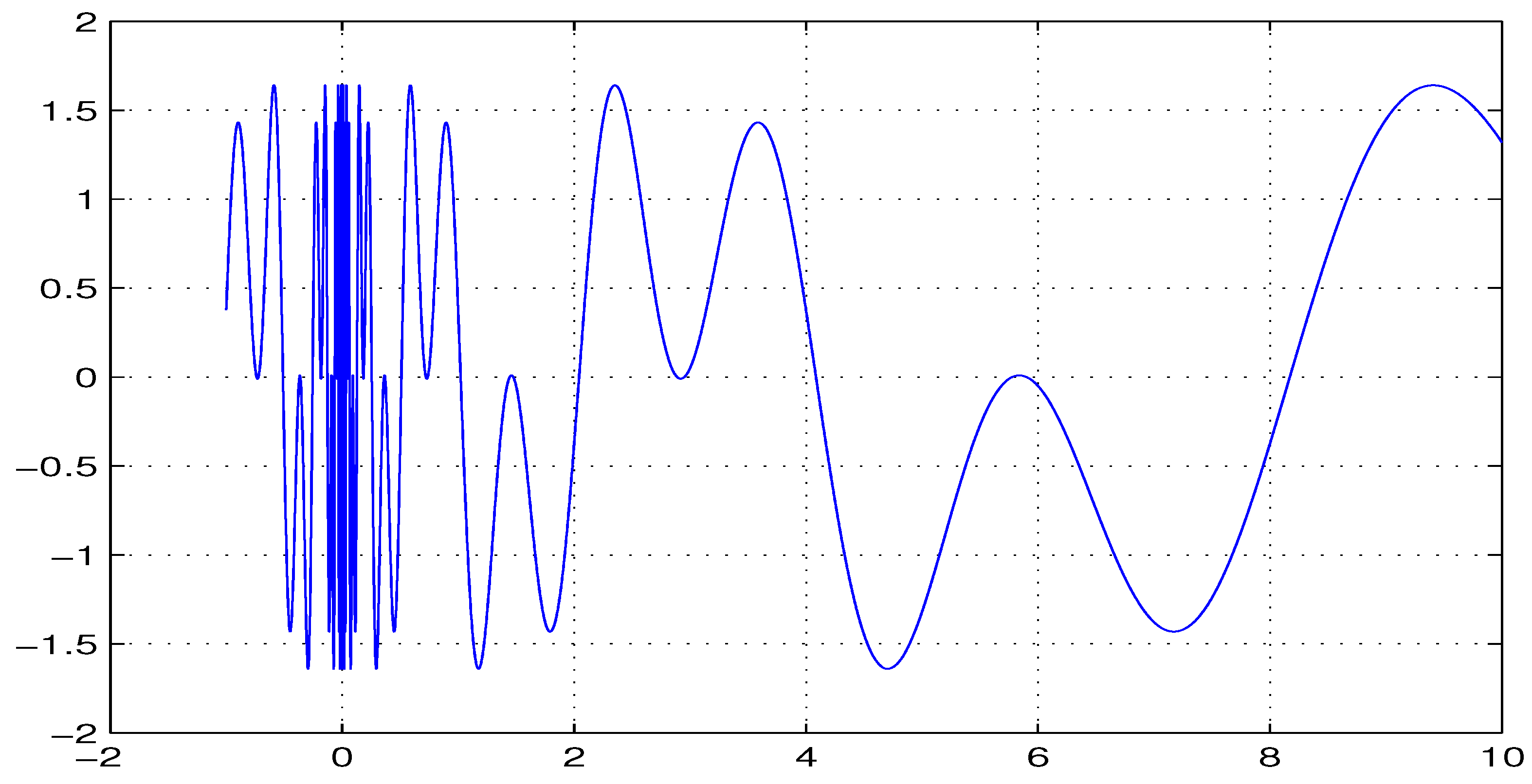
Step 2. Almost periodic function construction. Based on Step 1, consider the function
where and , then we obtain that is almost periodic. From Step 1, let
we obtain that . Note that and are periodic with different periods , respectively (see Figure 1).
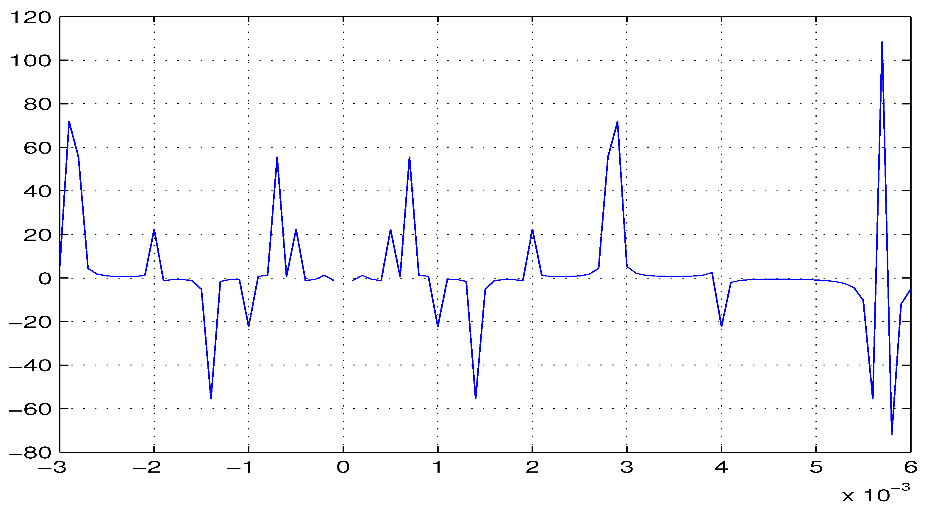
Step 3. -almost automorphic function construction. According to the above, we construct the following function:
where and , then is almost automorphic under the matched space . From Step 2, it follows that (see Figure 2).
Next, we construct an -almost automorphic function through -almost periodicity.
Example 2.
Step 1. -periodic function construction. For any , consider the real valued function whose domain is , then is Δ-periodic with the period under the matched space . In fact,
Step 2. -almost periodic function construction. On , let and
From Step 1, we have . Note that
Hence, is a -almost periodic function under the matched space and and have completely different periods.
Step 3. -almost automorphic function construction. According to Step 2, on , consider the following function on :
then is almost automorphic under the matched space . From Step 2, it follows that .
Remark 12.
From Examples 1–2, it demonstrates that Definitions 8 and 10 not only include the concepts of almost automorphic functions on periodic time scales under translations but also cover some new types of almost automorphic functions so almost automorphic problems for q-difference equations and others can be proposed and studied.
In what follows, for the convenience of our discussion, we always assume that is -differentiable and the time scale satisfies Definition 6, i.e., and .
Let be a Banach space endowed with the norm . Now denotes the Banach space of all bounded linear operators from to , if . Also is the space of bounded continuous function from to equipped with the supremum norm
Lemma 2.
If is Δ-differentiable for , then equipped with the norm is a Banach space.
Proof.
Let be a Cauchy sequence. Since is a Banach space, we can obtain . Hence, for any , there is a so that implies
Because , for each and , there exists a and so that , for any sequence , there is a subsequence such that
Now, take , and when , we obtain
We can take such that
which means that . Hence, is a Banach space equipped with the norm . □
Let U be the set of all functions which are positive and be locally integrable over for and .
Remark 13.
Note that, if or , then is positive and locally integrable over .
Remark 14.
Since by from Definition 4, then for . Hence, if is Δ-differentiable and , then is locally integrable over is equivalent to the local integrability of over .
For a given , set
for each
Remark 15.
Under a regular matched space , from Definition 7, we have i.e.,
In particular, if , then , and, in this case, we say Label (6) is the standard weighted function and
which is independent of . Throughout the paper, we assume that is a regular matched space and employ the standard weighted function (7).
Remark 16.
For any fixed and , if , then and . Hence, under a regular matched space , we have if .
Let and for any function , we use the notation .
Define
and
It is clear that
Now, for , define
Similarly, we define as the collection of all functions continuous with respect to its two arguments and is bounded for each and
uniformly for where .
Lemma 3.
If is Δ-differentiable for , then equipped with the norm is a Banach space.
Proof.
Let be a Cauchy sequence in . Then, for any , there is a such that implies
which indicates that is also a Cauchy sequence. Since is a Banach space, so we have as Therefore, from the definition of , we obtain . This completes the proof. □
Definition 14.
The sets and of standard -order weighted pseudo -almost automorphic functions are introduced as follows:
and we say is the main part of f.
From the Definition of , the following lemma is immediate:
Lemma 4.
Let be a regular matched space and is Δ-differentiable for all . If with a standard -almost automorphic function , and where , then
Proof.
We prove it by contradiction. Assume that the claim does not hold. Then, there exist a and such that Since , fix and and set . According to Lemma 2.1.1 of [35], there exist such that . Without loss of generality, we assume that and . Let
where , then and . For with and
one has
Thus,
Using the fact that , , we obtain
where .
On the other hand, from the triangle inequality, for any , one has
Then,
where since . This is a contradiction since . Hence, the claim is true. This completes the proof. □
In the following, we introduce the following function space:
Remark 17.
From Lemmas 2–3, we can easily obtain that and are also Banach spaces equipped with the norm .
Theorem 2.
Let be a regular matched space. Assume that is shift invariant under the matched space . Then, the decomposition of a main part for a standard -order weighted pseudo -almost automorphic function as is unique for any .
Proof.
Assume that and Then, Since and and in view of Lemma 4, we deduce that Consequently, that is, The proof is complete. □
Theorem 3.
Let be a regular matched space. Assume that is shift invariant and . Then, is a Banach space.
Proof.
Assume that is a Cauchy sequence in We can write uniquely . Using Lemma 4, we see that: from which we deduce that is a Cauchy sequence in the Banach space Thus, is also a Cauchy sequence in the Banach space We deduce that and finally The proof is complete. □
Definition 15.
Let One says that equivalent to , denoting this as if
Let It is the fact that (reflexivity); if then (symmetry), and if and then (transitivity). Thus, ≺ is a binary equivalence relation on
Theorem 4.
Let be a regular matched space and If , then
Proof.
Assume that There exists such that Thus,
where , and
The proof is complete. □
Lemma 5.
Let be a regular matched space and Then, where if and only if for every ,
where and
Proof.
- (a)
- Necessity. By contradiction, we suppose that there exists such thatThen, there exists such that, for every for some , whereAs a result, we getwhere This contradicts the assumption.
- (b)
- Sufficiency. Assume that Then, for every there exists such that for every ,where andNow, we haveTherefore, that is
The proof is complete. □
Lemma 6.
Let be a regular matched space. If and are standard -almost automorphic functions, then is standard -almost automorphic.
Proof.
From , then for every sequence of real numbers we can extract a subsequence such that:
is well defined for each . In view of assumption in our definition and , one can extract such that
Hence, is standard -almost automorphic. The proof is complete. □
We introduce two hypotheses as follows:
- (H1)
- is uniformly continuous in uniformly for any bounded subset .
- (H2)
- is uniformly continuous in uniformly for any bounded subset .
Theorem 5.
Let where is standard -almost automorphic, . Assume that and are satisfied. Then, the if , where .
Proof.
We have where and and where and
Now, let us write
From Lemma 6, Consider now the function
Clearly For to be in it is sufficient to show that
From Lemma 4, which is a bounded set. Using assumption with we say that for every , there exists such that
Thus, we obtain
Now, since then, by Lemma 5, Consequently,
Thus,
Finally, we need to show that Note that is uniformly continuous on and that is compact since is continuous on as an almost automorphic function. Thus, given there exists such that where for some and
Note that the set is open in and that Define by
Then, , if Thus, we get
In view of Label (8), it follows that
Thus, we get
Now, since and it follows that
i.e., The proof is complete. □
From Theorem 5, we can establish the following consequence:
Corollary 1.
Let where and assume both and are Lipschitzian in uniformly in . Then, if
3. Applications
Let be a regular matched space for the time scale , and consider the following linear dynamic equation
where is a linear operator in the Banach space .
Definition 16
([17]). is called the linear evolution operator associated with (9) if satisfies the following conditions:
- (1)
- ,where denotes the identity operator in ;
- (2)
- (3)
- the mapping is continuous for any fixed
To obtain our results, we will introduce the following concepts.
Definition 17.
Let be a matched space. An evolution system is called δ-exponentially stable if for any fixed , there exists and such that
Remark 18.
From Definition 17, if an evolution system is called exponentially stable, then there exist projections for each such that
since
Consider the abstract differential equation
with the following assumptions:
- (H1)
- The family of operators in generates an -exponentially stable evolution system i.e., for any fixed , there exists and such thatand, for any sequence , there exists a subsequence such that
- (H2)
- where
- (H3)
- (H4)
Definition 18.
A mild solution to (10) is a continuous function satisfying
for all and for all where .
Lemma 7.
if and only if .
Proof.
Assume that . Then we obtain
so we get .
On the other hand, if , one can obtain
Thus, we obtain . This completes the proof. □
To investigate the existence and uniqueness of a weighted pseudo -almost automorphic solution to (10), we need the following two lemmas:
Lemma 8.
Let be a regular matched space and be Δ-differentiable for all . Assume is a standard -almost automorphic function and is satisfied. If is the function defined by
then is a standard -almost automorphic function.
Proof.
Clearly, is a continuous functions. Let be an arbitrary sequence of real numbers. Since v is -almost automorphic, there exists a subsequence such that is well defined for each .
Now, we consider
where In addition, we have
Note that
for each fixed and any and we get
by the Lebesgue’s dominated convergence theorem. Analogous to the above proof, we can obtain
This shows that is a standard -almost automorphic function. The proof is complete. □
Lemma 9.
Let be a regular matched space and be Δ-differentiable for fixed . Let , where . Furthermore, are satisfied and is exponentially stable. Then,
Proof.
Let , where
Then, by Lemma 8, Now, we show that First, take such that , and by Remark 15, we have , it follows from Theorem 2.15 in [34] that
where
and
One can obtain
Since by Lemma 7, then
Hence, . The proof is complete. □
Theorem 6.
Let be a regular matched space and be Δ-differentiable for . Under assumptions above, (10) has a unique mild solution in provided .
Proof.
Consider the nonlinear operator given by
From Lemma 5, we see maps into .
Now, if , we have
Thus,
Hence, the conclusion follows from the contraction principle. The proof is complete. □
Corollary 2.
Suppose hold. Furthermore,
Then, (10) has a unique mild solution in provided .
Proof.
From (11), we can obtain
Let , and according to Theorem 6, we obtain the desired result. The proof is complete. □
4. An Example
Let be a regular matched space and be an arbitrary time scale with and , where is the following time scale:
Then, one will obtain that
where and , . Consider the following partial dynamic equation:
where satisfies and
Define , let Clearly, it follows from the same discussion as Section 3.1. in [36], one can obtain that the evolution system satisfies . Then, for all , by Lemma 3.3 from [21], we have
Let and
Clearly, for , f satisfies the assumptions given in Theorem 6 with
Therefore, (12) has the unique weighted pseudo -almost automorphic mild solution for .
5. Conclusions, Further Discussion and Open Problems
In this paper, using matched spaces for time scales, the properties of the complete-closed time scales under non-translational shift are established, and a wider range of irregular time scales turns into regular ones with “periodicity”. Then, the concepts of -order -almost automorphic functions and weighted pseudo -almost automorphic functions are introduced, and some basic theorems are obtained for weighted pseudo -almost automorphic functions and are then applied to investigate abstract dynamic equations. In addition, some sufficient conditions are derived to guarantee the existence of weighted pseudo -almost automorphic solutions for a new type of abstract dynamic equations. The obtained results develop a new almost automorphic theory for abstract dynamic equations involving quantum-like dynamic equations like q-difference dynamic equations and others.
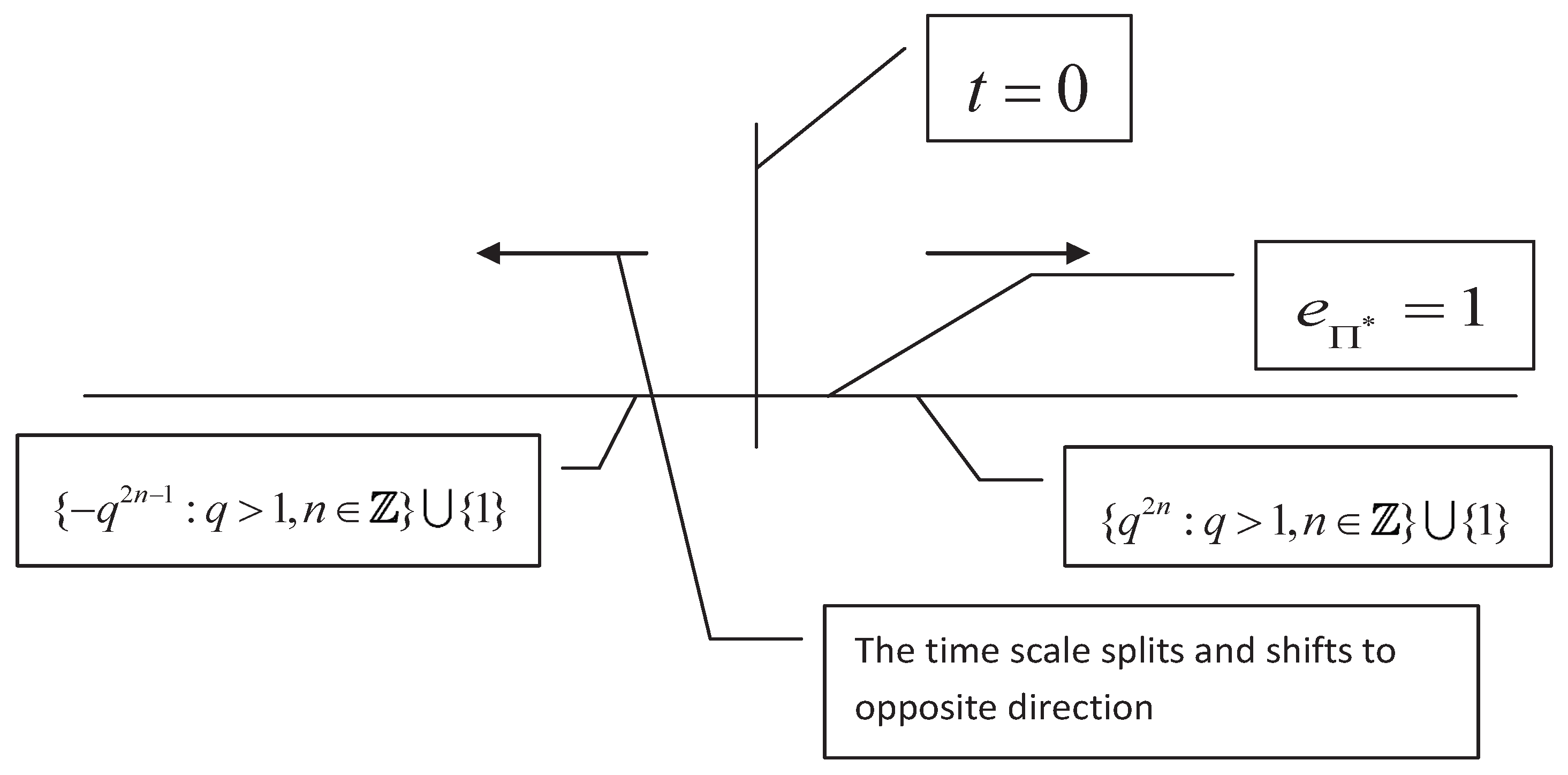
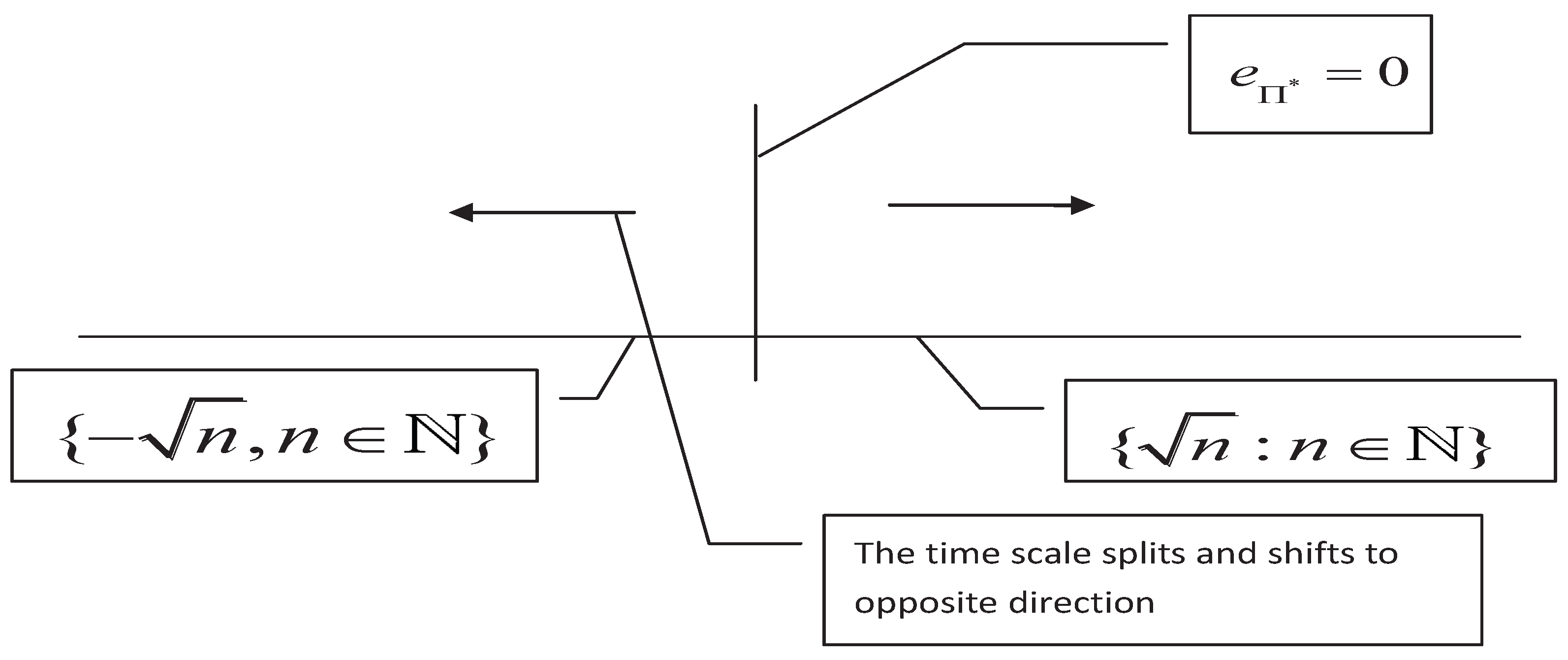
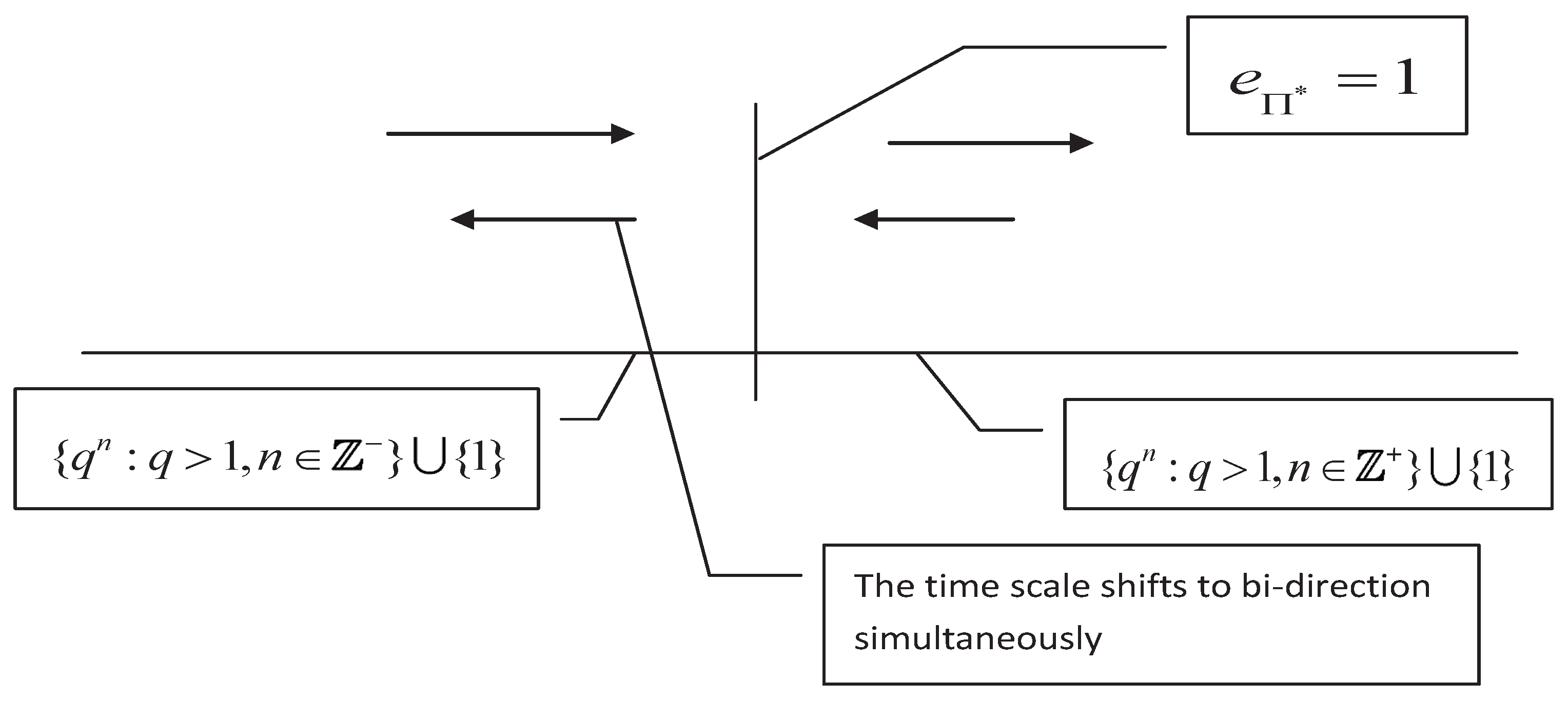
For the matched space , the shift operator may have the discontinuous point at some for (we call it characteristic point of the time scale under this matched space), particularly, if , then may be a characteristic point. For example, the time scales and have the characteristic points and (see Figure 3 and Figure 4), repectively. The characteristic points will lead to splitting of time scales, for example, the time scales and have the split point . From Figure 3, one will see that the characteristic point is , but the splitting point is , which implies that the characteristic point and the splitting point may not be equivalent (they may equal to each other, see Figure 4). However, if is continuous for all , then may have no characteristic point, it indicates that will not split and have the bidirectional shift closedness, see Figure 5.
For the above discussion, we propose the following open problems in a matched space .
- (i)
- What is the relationship between the characteristic points and the split points ?
- (ii)
- How many characteristic points and split points will a time scale have under a matched space?
- (iii)
- What is the relationship between the continuity of the shift operator and the shift closedness of different parts of the time scale?
Author Contributions
All authors contributed equally to the manuscript and typed, read and approved the final manuscript.
Funding
This work is supported by Youth Fund of NSFC (No. 11961077, No. 11601470) and Dong Lu Youth Excellent Teachers Development Program of Yunnan University (No. wx069051), IRTSTYN and Joint Key Project of Yunnan Provincial Science and Technology Department of Yunnan University (No. 2018FY001(-014)).
Acknowledgments
We express sincere thanks to all the reviewers’ comments and valuable suggestions to improve this manuscript.
Conflicts of Interest
The authors declare that they have no conflicts of interest.
References
- Bochner, S. A new approach to almost periodicity. Proc. Nat. Acad. Sci. USA 1962, 48, 2039–2043. [Google Scholar] [CrossRef] [PubMed]
- N’Guérékata, G.M. Topics in Almost Automorphy; Springer: New York, NY, USA, 2005. [Google Scholar]
- Ezzinbi, K.; N’Guérékata, G.M. Almost automorphic solutions for some partial functional differential equations. J. Math. Anal. Appl. 2007, 328, 344–358. [Google Scholar] [CrossRef]
- Goldstein, J.A.; N’Guérékata, G.M. Almost automorphic solutions of semilinear evolution equations. Proc. Am. Math. Soc. 2005, 133, 2401–2408. [Google Scholar] [CrossRef]
- N’Guérékata, G.M. Existence and uniqueness of almost automorphic mild solutions to some semilinear abstract differential equations. Semigroup Forum 2004, 69, 80–86. [Google Scholar] [CrossRef]
- Ezzinbi, K.; Fatajou, S.; N’Guérékata, G.M. Pseudo almost automorphic solutions to some neutral partial functional differential equations in Banach spaces. Nonlinear Anal. TMA 2009, 70, 1641–1647. [Google Scholar] [CrossRef]
- Liang, J.; N’Guérékata, G.M.; Xiao, T.J.; Zhang, J. Some properties of pseudo-almost automorphic functions and applications to abstract differential equations. Nonlinear Anal. TMA 2009, 70, 2731–2735. [Google Scholar] [CrossRef]
- Xiao, T.J.; Liang, J.; Zhang, J. Pseudo almost automorphic solutions to semilinear differential equations in Banach spaces. Semigroup Forum 2008, 76, 518–524. [Google Scholar] [CrossRef]
- Chang, Y.K.; Feng, T.W. Properties on measure pseudo almost automorphic functions and applications to fractional differential equations in Banach spaces. Electr. J. Differ. Equ. 2018, 47, 1–14. [Google Scholar]
- Chang, Y.K.; Tang, C. Asymptotically almost automorphic solutions to stochastic differential equations driven by a Lévy proces. Stochastics 2016, 88, 980–1011. [Google Scholar] [CrossRef]
- Chang, Y.K.; N’Guérékata, G.M.; Zhang, R. Existence of μ-pseudo almost automorphic solutions to abstract partial neutral functional differential equations with infinite delay. J. Appl. Anal. Comp. 2016, 6, 628–664. [Google Scholar]
- Blot, J.; Mophou, G.; N’Guérékata, G.M.; Pennequin, D. Weighted pseudo almost automorphic functions and applications to abstract differential equations. Nonlinear Anal. TMA 2009, 71, 303–309. [Google Scholar] [CrossRef]
- Diagana, T. Existence of weighted pseudo almost periodic solutions to some classes of hyperbolic evolution equations. J. Math. Anal. Appl. 2009, 350, 18–28. [Google Scholar] [CrossRef]
- Diagana, T. Existence of weighted pseudo-almost periodic solutions to some classes of nonautonomous partial evolution equations. Nonlinear Anal. TMA 2011, 74, 600–615. [Google Scholar] [CrossRef]
- Diagana, T. The existence of a weighted mean for almost periodic functions. Nonlinear Anal. TMA 2011, 74, 4269–4273. [Google Scholar] [CrossRef]
- Liang, J.; Xiao, T.J.; Zhang, J. Decomposition of weighted pseudo almost periodic functions. Nonlinear Anal. TMA 2010, 73, 3456–3461. [Google Scholar] [CrossRef]
- Wang, C.; Agarwal, R.P. Weighted piecewise pseudo almost automorphic functions with applications to abstract impulsive ∇-dynamic equations on time scales. Adv. Differ. Equ. 2014, 153, 1–29. [Google Scholar] [CrossRef]
- Wang, C.; Agarwal, R.P. Changing-periodic time scales and decomposition theorems of time scales with applications to functions with local almost periodicity and automorphy. Adv. Differ. Equ. 2015, 296, 1–21. [Google Scholar] [CrossRef]
- Wang, C.; Agarwal, R.P.; O’Regan, D. Periodicity, almost periodicity for time scales and related functions. Nonaut. Dyn. Syst. 2016, 3, 24–41. [Google Scholar] [CrossRef] [Green Version]
- Agarwal, R.P.; O’Regan, D. Some comments and notes on almost periodic functions and changing-periodic time scales. Electr. J. Math. Anal. Appl. 2018, 6, 125–136. [Google Scholar]
- Wang, C.; Agarwal, R.P. Uniformly rd-piecewise almost periodic functions with applications to the analysis of impulsive Δ-dynamic system on time scales. Appl. Math. Comput. 2015, 259, 271–292. [Google Scholar]
- Wang, C.; Agarwal, R.P. Almost periodic dynamics for impulsive delay neural networks of a general type on almost periodic time scales. Commun. Nonlinear Sci. Numer. Simul. 2016, 36, 238–251. [Google Scholar] [CrossRef]
- N’Guérékata, G.M.; Milce, A.; Mado, J.C. Asymptotically almost automorphic functions of order n and applications to dynamic equations on time scales. Nonlinear Stud. 2016, 23, 305–322. [Google Scholar]
- Kéré, M.; N’Guérékata, G.M. Almost automorphic dynamic systems on time scales. Panam. Math. J. 2018, 28, 19–37. [Google Scholar]
- Wang, C.; Agarwal, R.P.; O’Regan, D. n0-order Δ-almost periodic functions and dynamic equations. Appl. Anal. 2018, 97, 2626–2654. [Google Scholar] [CrossRef]
- Hilger, S. Ein Mafikettenkalkül mit Anwendung auf Zentrumsmannigfaltigkeiten. Ph.D. Thesis, Universität Würzburg, Würzburg, Germany, 1988. [Google Scholar]
- Bohner, M.; Peterson, A. Dynamic Equations on Time Scales; Birkhäuser Boston Inc.: Boston, MA, USA, 2001. [Google Scholar]
- Bohner, M.; Peterson, A. Advances in Dynamic Equations on Time Scales; Birkhäuser Boston Inc.: Boston, MA, USA, 2003. [Google Scholar]
- Adıvar, M. A new periodic concept for time scales. Math. Slovaca 2013, 63, 817–828. [Google Scholar] [CrossRef]
- Kaufmann, E.R.; Raffoul, Y.N. Periodic solutions for a neutral nonlinear dynamical equation on a time scale. J. Math. Anal. Appl. 2006, 319, 315–325. [Google Scholar] [CrossRef] [Green Version]
- Wang, C.; Agarwal, R.P. Almost periodic solution for a new type of neutral impulsive stochastic Lasota–Wazewska timescale model. Appl. Math. Lett. 2017, 70, 58–65. [Google Scholar] [CrossRef]
- Wang, C.; Agarwal, R.P.; O’Regan, D. A matched space for time scales and applications to the study on functions. Adv. Differ. Equ. 2017, 305, 1–28. [Google Scholar] [CrossRef]
- Cabada, A.; Vivero, D.R. Expression of the Lebesgue Δ-integral on time scales as a usual Lebesgue integral; application to the calculus of Δ-antiderivatives. Math. Comput. Model. 2006, 43, 194–207. [Google Scholar] [CrossRef]
- Bohner, M.; Guseinov, G.S. Double integral calculus of variations on time scales. Comput. Math. Appl. 2007, 54, 45–57. [Google Scholar] [CrossRef] [Green Version]
- Veech, W.A. Almost automorphic functions on groups. Am. J. Math. 1965, 87, 719–751. [Google Scholar] [CrossRef]
- Jackson, B. Partial dynamic equations on time scales. J. Comput. Appl. Math. 2006, 186, 391–415. [Google Scholar] [CrossRef] [Green Version]
Figure 1.
Graph of with .

Figure 2.
Graph of with .

Figure 3.
The time scale has the characteristic point at which the shift is discontinuous. This time scale splits at and has the opposite shift closedness at the split point.
Figure 3.
The time scale has the characteristic point at which the shift is discontinuous. This time scale splits at and has the opposite shift closedness at the split point.

Figure 4.
The time scale has the characteristic point at which the shift is discontinuous. This time scale splits at and has the opposite shift closedness at the split point.
Figure 4.
The time scale has the characteristic point at which the shift is discontinuous. This time scale splits at and has the opposite shift closedness at the split point.

Figure 5.
The time scale has the characteristic point at which the shift is continuous. This time scale has the bidirectional shift closedness.
Figure 5.
The time scale has the characteristic point at which the shift is continuous. This time scale has the bidirectional shift closedness.

© 2019 by the authors. Licensee MDPI, Basel, Switzerland. This article is an open access article distributed under the terms and conditions of the Creative Commons Attribution (CC BY) license (http://creativecommons.org/licenses/by/4.0/).
Share and Cite
MDPI and ACS Style
Wang, C.; Agarwal, R.P.; O’Regan, D.; N’Guérékata, G.M. n0-Order Weighted Pseudo Δ-Almost Automorphic Functions and Abstract Dynamic Equations. Mathematics 2019, 7, 775. https://0-doi-org.brum.beds.ac.uk/10.3390/math7090775
AMA Style
Wang C, Agarwal RP, O’Regan D, N’Guérékata GM. n0-Order Weighted Pseudo Δ-Almost Automorphic Functions and Abstract Dynamic Equations. Mathematics. 2019; 7(9):775. https://0-doi-org.brum.beds.ac.uk/10.3390/math7090775
Chicago/Turabian StyleWang, Chao, Ravi P. Agarwal, Donal O’Regan, and Gaston M. N’Guérékata. 2019. "n0-Order Weighted Pseudo Δ-Almost Automorphic Functions and Abstract Dynamic Equations" Mathematics 7, no. 9: 775. https://0-doi-org.brum.beds.ac.uk/10.3390/math7090775
Note that from the first issue of 2016, this journal uses article numbers instead of page numbers. See further details here.