Applications of the Fractional Diffusion Equation to Option Pricing and Risk Calculations


1
BRED Banque Populaire, Modeling Department, 18 quai de la Râpée, 75012 Paris, France
2
Section for the Science of Complex Systems, Center for Medical Statistics, Informatics, and Intelligent Systems (CeMSIIS), Medical University of Vienna, Spitalgasse 23, 1090 Vienna, Austria
3
Complexity Science Hub Vienna, Josefstädterstrasse 39, 1080 Vienna, Austria
4
Faculty of Nuclear Sciences and Physical Engineering, Czech Technical University, 11519 Prague, Czech Republic
5
Beuth Technical University of Applied Sciences Berlin, Luxemburger Str. 10, 13353 Berlin, Germany
*
Author to whom correspondence should be addressed.
Mathematics 2019, 7(9), 796; https://0-doi-org.brum.beds.ac.uk/10.3390/math7090796
Submission received: 15 August 2019
/
Revised: 26 August 2019
/
Accepted: 26 August 2019
/
Published: 1 September 2019
(This article belongs to the Special Issue Mathematical Economics: Application of Fractional Calculus)
Abstract
:In this article, we first provide a survey of the exponential option pricing models and show that in the framework of the risk-neutral approach, they are governed by the space-fractional diffusion equation. Then, we introduce a more general class of models based on the space-time-fractional diffusion equation and recall some recent results in this field concerning the European option pricing and the risk-neutral parameter. We proceed with an extension of these results to the class of exotic options. In particular, we show that the call and put prices can be expressed in the form of simple power series in terms of the log-forward moneyness and the risk-neutral parameter. Finally, we provide the closed-form formulas for the first and second order risk sensitivities and study the dependencies of the portfolio hedging and profit-and-loss calculations upon the model parameters.
1. Introduction
Fractional Calculus (FC) is nearly as old as conventional calculus. Many prominent mathematicians including Leibniz, Fourier, Laplace, Liouville, Riemann, Weyl, and Riesz suggested their own definitions of the fractional integrals and derivatives and studied their properties. Whereas the mathematical theory of FC was nearly completed a long time ago (see, e.g., [1] or the recent reference books [2,3]), only a few applications of FC outside mathematics were known until recently. During the last three decades, the situation changed completely, and currently, the majority of FC publications is devoted to modeling of a broad class of systems and processes using either the FC operators or the so-called fractional ordinary or partial differential equations. In particular, the FC models were successfully employed in physics [4,5], control theory [6], as well as in engineering, life, and social sciences [7,8], to mention only a few of the many application areas.
The two probably most prominent and broadly-recognized FC applications are in linear viscoelasticity [9] and for describing anomalous transport processes [10]. In both cases, the FC models in the form of the fractional ODEs (linear viscoelasticity) and the fractional PDEs (anomalous transport processes), respectively, cannot be derived from “first principles”. Instead, they are introduced as interpolations between several models formulated in terms of the ODEs or PDEs, respectively. In the case of linear viscoelasticity, the basic FC model interpolates between the Hooke model (elasticity, ODE of the zero order) and the Newton model (viscosity, ODE of the first order). The FC model for the slow anomalous diffusion interpolates between a stationary state (time-independent Poisson equation) and the diffusion equation (first order equation with respect to time), whereas the fast diffusion is modeled by the fractional diffusion-wave PDE that interpolates between the diffusion equation (first order equation with respect to time) and the wave equation (second order equation with respect to time).
Of course, this kind of model needs an additional justification, say, in the form of a better fitting of certain datasets or better predictions compared to ones delivered by the conventional models. One of the advantages of the FC models is that they have some additional parameters (orders of the fractional derivatives) that can be suitably chosen for a set of data at hand. To do this, an inverse problem for the determination of the optimal parameters from the data has to be solved (see, e.g., [11] for an excellent survey of the basic inverse problems for the fractional differential equations).
It is worth mentioning that the anomalous diffusion models have a clear stochastic interpretation and can be formulated in terms of the continuous time random walk processes. The models in the form of the time- and/or space-fractional differential equations follow from these stochastic models for a special choice of the jump probability density functions with infinite first or/and second moments [10,12,13]. In [14], the fundamental solution for a time-fractional diffusion equation with the Caputo fractional derivative of order and the spatial Laplace operator was shown to be a probability density function evolving in time. In [15], a space-time fractional diffusion equation with the spatial Riesz–Feller derivative of order and skewness () and the time-fractional Caputo derivative of order was investigated in detail. In particular, several subordination formulas for the fundamental solutions of this equation with different values of and and an extension of their probabilistic interpretation to the ranges and were derived in [15].
A close connection of the fractional diffusion equations with the stochastic processes (fractional Brownian motion, Lévy flights, etc.) made them very promising models for different financial applications. In particular, they were already employed in the hot problems of finance (for recent reviews, see, e.g., [16,17]), particularly in financial markets [18,19,20,21], macroeconomics [22], mathematical economics [23], and for describing the concept of memory in economics [24] or economic growth [25]. One of the first applications of FC in finance was through the fractional Brownian motion, which enables incorporating long-range auto-correlations, typically observed in finance [26,27], volatility modeling [28], and option pricing [29]. FC has been specifically used in many option pricing models [30,31,32,33], also in connection with the jump processes [34] or in pricing of more complicated types of options, as American options [31], double barrier options [35], or currency options [36]. These models have been also investigated by numerical methods [37,38], and some applications to implied volatility have been also discussed [39].
In this paper, we focus on FC applications to option pricing, which is one of the most important tasks of financial mathematics. It is an important tool for market participants who want to hedge their positions and to estimate the value and risks or their portfolios. The first option pricing model was introduced by Black and Scholes [40] in 1973 based on the Gaussian assumptions for the variation of the stock prices’ returns. After that, many generalizations and adaptations of this model were derived in order to capture the behavior of financial markets more realistically (let us mention, among others, models based on stochastic volatility [41], regime switching [42], or jumps [43]). Particularly interesting are the approaches based on replacement of the underlying stochastic process by the fractional Brownian motion or Lévy flights that leads to models driven by the fractional diffusion equations. One of the first models of this kind explicitly designed for the purpose of option pricing was introduced by Carr and Wu [44] by replacing the conventional Gaussian noise by a maximally-skewed Lévy-stable process (in other words, by replacing the underlying diffusion equation by a space-fractional diffusion equation). This model is far more realistic than the Black-Scholes model because it incorporates the heavy-tailed distributions and thus allows reproducing complex, but observable behavior in the distribution of prices (such as large drops) and in long-term volatility patterns. In this paper, we focus on a generalization of this model based on the space-time fractional diffusion equation [15] originally introduced in [45] and further investigated in [46,47,48,49]. The main advantage of this model is its interpretation: the model parameters play the role of the volatility (general risk level) and the spatial and temporal risk redistributions, and therefore, this model captures the complex market behaviors more accurately compared to the conventional models. In the first part of this paper, we recall the main features and particular cases of the fractional diffusion model, as well as some recent results on European option pricing. Then, we apply this mathematical framework to more exotic types of options, i.e., binary options. The second part of the paper is devoted to the risk sensitives and Profits and Losses (P&L) calculations, which are very important for market practitioners.
The paper is organized as follows. In Section 2, we provide an overview of some recent results on fractional diffusion models and discuss their applications to financial modeling. Section 3 is devoted to the pricing formulas for the European and binary options driven by the space-time fractional diffusion equation. In Section 4, we apply our results to the risk sensitivities and portfolio management. The last section is dedicated to the conclusions.
2. The Fractional Diffusion Model and Option Pricing
We start with some standard financial definitions. A call (resp. put) option with a strike and a maturity is a financial instrument that gives the holder the right to buy (resp. to sell) a given quantity S (an asset, an index, etc.) at an agreed price at time . We will denote the option payoff by .
In the case:
one speaks of an European call option. If the option has the payoff (1), but can be exercised at any time , one speaks of an American call option. European and American options are often referred to as the vanilla options, while the payoff of the so-called exotic options is determined by some more sophisticated algorithms. Say, the payoff of the binary or the digital call options is given by the formula:
where H denotes the Heaviside step function. Let us also mention that there are even more complicated options such as Asian or barrier options, which are path-dependent instruments. This means that the payoff of these options depends on all values of the asset price , , and not just on . In this paper, the focus is mainly on the European and binary options.
Evidently, in order to calculate the options’ prices, the dynamics of the underlying asset has to be described and modeled. A common way to do this is interpretation of as a stochastic process, so that the payoff function becomes a random variable with a certain probability distribution. In the next subsection, we discuss a particular class of stochastic models for , which are very popular among the market practitioners.
2.1. Exponential Market Models
In a wide class of option pricing models, it is assumed that the underlying asset price is described by a stochastic process on a filtered probability space , whose instantaneous variations can be written in local form as follows:
where r denotes the continuous risk-free interest rate and stands for the market volatility. For financial application, the common choices for are:
- Gaussian process: (standard Brownian motion). In this case, the stock price is said to follow a geometric Brownian motion. This is the basic hypothesis for the Black-Scholes model [40].
- Lévy process: (standardized Lévy-stable process with stability and skewness or asymmetry ). In this case, one says that follows an exponential Lévy-stable process (see the details in [43]). Exponential Lévy models generalize the Gaussian framework (because for any ), while allowing additional realistic features such as the presence of price jumps with non-zero probability. Their relevance in financial modeling has been known since the works of Mandelbrot and Fama [50,51]. For most financial applications, only the so-called Lévy-Pareto distributions, i.e., the values , are relevant (historically, Mandelbrot calibrated for the cotton market).
It is important to note that the stochastic differential Equation (3) is specified under the risk-neutral measure (also known as the martingale measure), that is the measure under which the discounted market price is a martingale (for more information regarding the risk-neutral option pricing, see [52] or any monograph on financial mathematics):
where . The martingale measure is given by the Esscher transform [53] of the physical measure :
where the parameter is defined as the value of the negative cumulant-generating function evaluated at the point 1:
In particular, if the process admits a probability distribution (or density) , then reads:
and therefore, the existence of a risk-neutral measure is linked to the existence of the two-sided Laplace transform of the density. As we will see later, for exponential Lévy models, the two-sided Laplace transform diverges with the only exception in the case when the asymmetry parameter is maximal, that is when the probability distribution has exponential decay on the positive real semi-axis and polynomial decay (heavy tail) on the negative real semi-axis.
With the above notations, the solution to (3) is the exponential process:
and the price of an option with strike K, maturity T, and payoff is equal to the present value of its expected payoff:
2.2. Generalizing Exponential Market Models: The Fractional Diffusion Model
2.2.1. Setup of the Model
By the space-time fractional diffusion model, we mean the following Cauchy problem:
where the parameters and are restricted as follows: , . The asymmetry parameter belongs to the so-called Feller-Takayasu diamond . denotes the Caputo fractional derivative, which is defined as:
and denotes the Riesz–Feller fractional derivative, which is usually defined via its Fourier image:
By definition, both fractional derivatives become ordinary derivative operators if the orders of the derivatives are natural numbers. The fundamental solution or the Green function of (11), that is the solution corresponding to the initial values and , was derived in [15] in form of a Mellin-Barnes integral (for ):
The Green function (14) can be extended to the negative values of the argument x due to the symmetry relation:
As an extension of the pricing formula for the exponential models (10), we now define the price of an option driven by the fractional diffusion model as follows:
Similarly to Equation (7), the risk-neutral parameter now reads:
It follows from (17) that the Green function has to admit an exponential decay on the positive semi-axis to ensure the existence of the risk-neutral parameter. This is the case as soon as the maximal negative asymmetry (or skewness) holds (see the next section for calculations of in the space- and time-fractional cases):
In what follows, we will denote the corresponding Green functions, the risk neutral parameters, and the call option prices as follows:
2.2.2. Financial Interpretation of the Parameters
The fractional diffusion models incorporate two new degrees of freedom (the order of the spatial derivative and the order of the time derivative ) that act as the risk redistribution parameters. More precisely, while the parameter in the model (3) represents the volatility of the returns of the underlying asset and, as such, has an equal impact on all kinds of options (an increase of leads to an increase of the price of both call and put options), any changes of the parameters and do not affect all options in the same direction.
For instance, as observed in [45], if , then the short-term options become more expensive and the long-term ones less expensive compared to the non-fractional case . This situation is observable when the market conditions are far from equilibrium (dramatic price jumps, exceptional events impacting the markets, etc.) and can be interpreted as a manifestation of memory [24]. The parameter plays therefore the role of a temporal redistribution. In this paper, we will show how it affects the profit and loss of a portfolio.
The parameter represents a spatial redistribution because it controls the heavy-tails of the probability distributions (see the discussion thereafter). Its impact has been extensively discussed in [44], where it was shown to be an excellent candidate for the long-term volatility modeling. Indeed, when the maturity increases, it is known that the volatility smirk does not flatten out as expected if the Gaussian hypothesis would be true. By letting vary between one and two, the negative slope of the smirk can be controlled. It is flat when (Gaussian case) and becomes steeper when decreases, thus generating any observable slope in equity index options markets (the impact of on the volatility structure for at-the-money option was discussed in [47]). In this paper, we will also prove that the parameter governs the delta-hedging policy of the portfolios, that is the way of constructing portfolios whose values are independent of the fluctuations in the stock price .
Finally, let us mention that a calibration of the model parameters from the traded options for a one-month trading period was suggested in [45] for the European calls and puts (together and separately). The results of calibration showed that fluctuated around 1.5 and 1.6 (therefore, rather far from the Gaussian hypothesis, but close to the Mandelbrot estimates) and that , although close to one, varied simultaneously with and in the same direction as . This leads to a relative stability for the diffusion scaling exponent .
2.3. Particular Cases
In this subsection, we discuss some well-known exponential models (3) that are particular cases of the fractional diffusion model (16).
2.3.1. Finite Moment Log Stable model
In the framework of the Finite Moment Log Stable (FMLS) model [44], the stochastic process driving the stock price dynamic (3) is given by:
where is a standardized Lévy-stable process (see [43]) with stability and asymmetry (or skewness) , whose probability distribution is the so-called stable distribution [54]. As already mentioned, this model was introduced by Carr and Wu in order to capture the behavior of the volatility smirk (the phenomenon that, for a given maturity, implied volatility is higher for out-of-the-money puts than for out-of-the-money calls): as a function of moneyness, it is widely observed that the smirk does not flatten out for longer observable horizons (i.e., greater than two years), and this can only be achieved if one violates the Gaussian hypothesis. The maximal negative hypothesis ensures the existence of a risk-neutral parameter: indeed, the two-sided Laplace transform of the stable distribution exists only if , with the result [55]:
Therefore, from a symmetry argument, the risk-neutral parameter exists and is finite only if . It follows from (21) that its value is given by the formula:
where was introduced as a normalization constant to recover the Black-Scholes factor for :
Moreover, under the condition , the probability distribution has a fat tail on the negative real axis as soon as (that is, it decays as ) and decays exponentially on the positive real axis. This highly-skewed behavior could not be captured by a traditional Brownian motion and by any symmetric distribution. However, it is a very plausible assumption as large drops are far more commonly observed in financial markets than large rises.
The FMLS model is actually a particular case of the fractional diffusion model: indeed, the choice is the probabilistic equivalent of the choice (18), and the probability distribution is the Green function associated with the space-fractional diffusion equation ():
From the pricing Formula (16), the option price in the framework of the FMLS model reads:
where the Green function is given by the formula:
Recently, an analytic option pricing formula for the FMLS model in the case of European options was derived in [48] in the form of a fast convergent double series. In the present paper, we extend this formula to the case of a time-fractional derivatives in (24), that is for , and to other types of options.
2.3.2. Black-Scholes Model
The celebrated Black-Scholes model [40] assumes that the stochastic process driving the exponential model (3) is a standard Brownian motion, i.e., . This model turns out to be a particular case of the FMLS model (and therefore, of the fractional diffusion model) because for , the Lévy-stable process degenerates into for any . It is well known that the probability distribution of the Wiener process is the Green function associated with the diffusion equation:
which is known to be the Gaussian kernel:
As expected, the diffusion Equation (27) is a particular case of the space-fractional diffusion Equation (24) for and with the Gaussian risk-neutral parameter (23). Using the pricing Formula (16), the price of the option in the Black-Scholes model reads:
For , some elementary manipulations on the integral (29) lead to the Black-Scholes formula for the European options, which, in our system of notations, reads as follows:
where is the standard normal cumulative distribution function, and the forward strike priceF and the log-forward moneynessk are defined by the expressions:
3. Pricing Formulas
3.1. Risk-Neutral Parameter
In general, the risk-neutral parameter is not known in the analytic form as soon as . However, it has been shown in [46] that can be expressed in terms of a Mellin-Barnes integral involving the FMLS risk-neutral parameter (which is known in explicit form):
Proposition 1.
Let and . Then, for any , the formula:
holds true.
Under some conditions on and , the right-hand side of the integral representation (32) can be expressed as a series:
Theorem 1.
Let . If , then the series representation:
is valid.
Proof.
The Stirling asymptotic formula for the Gamma function (see [56]) leads to the following statement ():
Applying it to the integrand in the integral representation (32) under the condition , we can evaluate the integral along the vertical line by closing the contour in the right-half plane because it will not contribute when . In this region, the function is singular every time its argument equals a negative integer , that is when , with residue (see the details in [56] or [57]). Therefore, we get the formula:
Summing all residues and applying the residue theorem complete the proof. ☐
An important approximation to the risk-neutral series (33) is easily obtained via the Taylor series for :
Now, it follows from the reflection formula for the Gamma function that one can re-write the FMLS risk-neutral parameter (22) as follows:
Plugging the last formula into Formula (36), we have the following result:
Corollary 1.
Let and . Then, the formula:
holds true.
In particular, in the case of the fractional Black-Scholes model (), we get the expression:
which resumes to the well-known Gaussian parameter when .
3.2. European Options
Let us denote by the price of the European call option in the fractional diffusion model with the payoff .
Proposition 2.
Let P be the polyhedron . Then, for any vector ,
Proof.
First, we mention that under the maximal negative asymmetry hypothesis and on the positive real axis, the Green function (14) has the form:
On the other hand, using the notations (31), we can rewrite the payoff function in the form:
then integrate by parts over the variable x, and get the expression:
The Mellin-Barnes representation for the exponential term (see [58] or any other monograph on integral transforms) reads:
The relation along with some elementary simplifications yields the integral representation (40). ☐
Let us now represent the Mellin-Barnes double integral (40) in terms of a double series by means of residue summation.
Theorem 2 (Pricing formula: European call).
Let and . Then, under the maximal negative asymmetry hypothesis (), the price of the European call driven by the space-time fractional diffusion equation is as follows:
Proof.
Let denote the differential form in the integral at the right-hand side of (40). If we perform the change of the variables:
then reads:
In the region , has a simple pole at every point , with the residue:
The pricing Formula (46) is a simple and efficient way for the calculation of the pricing of the European call options. The convergence of the partial sums in the double series (46) is very fast, and therefore, only a few terms are needed to obtain an excellent level of precision (see numerical applications and convergence tests in [46,47]). As a particular case of the pricing Formula (46) with , we recover the pricing formula for the FMLS model that was established in [48]:
If we set in the last formula, then we obtain the series expansion for the Black-Scholes European call:
where . In [59], using the change of variables and the properties of the Gamma function, it was proven that (51) can be ordered in odd powers of Z:
A particularly interesting situation occurs when the asset is At-The-Money (ATM) forward, that is when or equivalently with our notations in Equation (46). In this case, we get the following result:
Corollary 2 (At-the-money price: European call).
For , the price of the European call option driven by the space-time fractional diffusion equation is given by the formula:
As a particular case of (53), the ATM price in the FMLS model reads:
as was already established in [48]. When , we get:
As , we have thus recovered the well-known Brenner–Subrahmanyam approximation for the European Black-Scholes call (which was first introduced in [60]):
3.3. Binary (or Digital) Options
3.3.1. Cash-or-Nothing
Let us denote by the price of the binary cash-or-nothing option in the fractional diffusion model with the payoff .
Proposition 3.
For any , the formula:
holds true.
Proof.
Inserting the terminal payoff into the call price (16) yields:
Performing the integration with respect to the x-variable and using the relation yield the representation (57). ☐
Theorem 3 (Pricing formula: cash or nothing call).
Let and . Then, under the maximal negative asymmetry hypothesis (), the price of the cash-or-nothing call option driven by the space-time fractional diffusion equation is given by the formula:
Proof.
As , it follows from Formula (34) that the line integral in (57) can be expressed as a sum of the residues induced by the poles of the function. These poles are located at the points , and the associated residues are as follows:
Summing up all residues completes the proof. ☐
In the particular case of the Black-Scholes model (,), the series (59) has only the odd terms because of the divergence of the denominator at negative integers. Using the known values of the Gamma function at the half-integers, we then obtain the formula
Let us now consider the cash-or-nothing put option .
Proposition 4.
For any , the integral representation:
holds true.
Proof.
The proof is similar to the one given for the proposition 3. The only difference is that one has to replace the payoff by and to consider the Green function on the negative real axis. Using the symmetry property (15), it reads as follows:
☐
The integral for the put price (62) needs more efforts than the integral for the call price (57). Indeed, it possesses two distinct series of poles in the positive half-plane:
- The poles of at the points , whose residues are given by the formula:
- The poles of at the points , whose residues are given by the formula:
However, in the non-time-fractional case, it is possible to derive a simple representation for the put price.
Theorem 4 (Pricing formula: space fractional cash or nothing put).
Let . Then, under the maximal negative asymmetry hypothesis (), the price of the cash-or-nothing call option driven by the space fractional diffusion equation is as follows:
Proof.
In the space-fractional case, the parameter is equal to one. Then, we have the following simplifications:
and the proof is complete. ☐
Note that in the space fractional case, the call Formula (59) can be written in the form:
and therefore, the sum of the space fractional call and put options is given by the formula:
The relation (71) is an example of a call-put parity relation. The fact, that it is independent of is not a surprise since, as already mentioned in the previous section, the space fractional model is equivalent to the FLMS model for which the option prices admit a risk-neutral representation:
3.3.2. Asset-or-Nothing
Let us denote by the price of the binary cash-or-nothing option in the fractional diffusion model with the payoff .
Proposition 5.
Let P be the polyhedron . Then, for any vector , the integral representation:
holds true.
Proof.
To prove the formula, we replace the payoff function in the option price Formula (16) by:
and then proceed exactly as in the proof of Proposition 2. ☐
Theorem 5 (Pricing formula: asset or nothing call).
Let and . Then, under the maximal negative asymmetry hypothesis (), the price of the asset-or-nothing call option driven by the space-time fractional diffusion equation is given by the formula:
Proof.
The series (80) is obtained by summing the residues associated with the poles of the functions and exactly in the same manner as in the proof of Theorem 2. ☐
As a consequence of Theorems 2, 3 and 5, the European call can be represented as a difference between an asset-or-nothing call and a cash-or-nothing call:
4. Risk Sensitivities and Portfolio Hedging
In quantitative finance, the risk sensitivities are also known as the “Greeks”. They quantify the dependence of an option on the market parameters such as the asset (spot) price or volatility and are essential tools for portfolio management. In this section, we derive for them some efficient representations and study how the orders of the time- and space-fractional derivatives impact the hedging policies.
4.1. First Order Sensitivity (Delta)
4.1.1. European Call
From the definition of k, we have the relation . Thus, by differentiation of (46) with respect to S and re-arranging the terms, we obtain the formula:
where we have used the definition (31) for the moneyness to deduce the relation . When the asset is ATM forward (, and therefore, ), Formula (82) can be simplified:
Equation (83) shows that the Delta of at-the-money calls is driven by (see also Figure 1), which generalizes the well-known feature of the Black-Scholes model, where at-the-money call options have a Delta of . In particular, (83) demonstrates that, at first order, only the space fractional parameter influences the delta-hedging policy of a portfolio. Indeed, it is sufficient to be long of one unit of the asset S and short of units of an European call to offset the impact of the variations of S:
where is the ATM forward price.
4.1.2. Cash-or-Nothing Call
In the at-the-money forward situation, we then get:
This formula can be simplified when (the so-called neutral diffusion). Using the known asymptotic behavior of the Gamma function at the point 0, we then get:
4.1.3. Cash-or-Nothing Put
In the space-fractional case (), it follows from the parity relation (71) that the cash-or-nothing call and put options have opposite Deltas:
4.1.4. Asset-or-Nothing Call
4.2. Second Order Sensitivity (Gamma, Dollar Gamma)
By the definition of k, . Thus, differentiation of (82) with respect to S along with a re-arrangement of the terms give the formula:
In the ATM forward situation, (93) is reduced to the form:
The leading term in the expression at the right-hand side of (94) is the following one:
Let us assume that we are long of one European call option and that we have delta-hedged our portfolio when (according to (84), this is made by being short of units of the asset S). We can then employ the Taylor formula to approximate the value of the portfolio when S varies:
The left-hand side of (96) is the Profit and Loss, or P& L of the portfolio around the money. As we have delta-hedged our position, this P&L is therefore essentially driven by the option’s convexity, and one speaks of Gamma P& L. For , we can use the approximation (39) of the risk-neutral parameter and its Taylor expansion with respect to to obtain the following easy-to-use P& L formulas ( denotes the Euler–Mascheroni constant):
- If :
- If :
- If :
The term is the square of the underlying asset’s returns and, as such, is interpreted as the realized variance. Its multiplicative factor is often called the dollar Gamma ($Γ). By definition, with our notations, it reads:
The Gamma P&L can therefore be written down in the form:
We can observe that, for any , the graph of the dollar Gamma remains positive and therefore works in favor of the long call position. In other words, the P&L of the call option will outperform the one of the hedge, because the option price is a convex function of the asset price. Thus, this well-known feature of the conventional Black-Scholes theory is preserved in the framework of the time-fractional diffusion model. The presence of the parameter , however, significantly affects the impact of option’s maturity to the Gamma P&L. As seen in (102), the Black-Scholes dollar Gamma is equal to and therefore is maximal for short-term options (i.e., for small ). However, when tends to zero, then tends to and becomes independent of . Similarly, when , the option will no longer outperform the hedge, and the P&L of the portfolio will remain flat, whatever the option’s maturity. This phenomenon illustrates the temporal redistribution induced by the time-fractional parameter . Finally, Figure 2 demonstrates that the Gamma P&L is a decreasing function of as soon as , and there is an inflection at the point :
5. Conclusions
In this article, we presented a theory of option pricing based on the fractional diffusion equation and showed that it constituted a generalization of the well-known class of the exponential market models. In particular, we extended the pricing formulas that were previously established for the vanilla options to a basic class of exotic options, computed the related risk sensitivities, and applied the results to delta-hedging and P&L calculations.
The pricing formulas were derived in the form of fast converging series of powers of the log-forward moneyness and of the risk-neutral parameter that generalizes the volatility parameter to the non-Gaussian case and also admits a convenient series representation. These series can be easily used for calculations in practice without the help of any sophisticated numerical tools. Moreover, they clearly exhibit the impact of the model parameters to risks and hedging: the order of the space derivative governs the delta-hedging of the portfolio, while the order of the time derivative drives the P&L of this portfolio.
Other important problems include the development and analysis of similar analytic tools for other types of commonly-traded payoffs (especially for the path-dependent options) and other types of financial derivatives. We also are going to apply these models to the real market data. In order to verify the effectiveness of our approach, we first need to determine the reliable estimations of the model parameters and then to compare the numerical results produced by the model with the market data. Another interesting problem concerns relaxing of the maximal asymmetry hypothesis. However, this would imply divergence of the risk-neutral expectations, and thus, some suitable re-normalization procedures such as, say, the cut-offs of the probability densities, would be probably needed to make progress in the solution of this problem.
Author Contributions
J.-P.A. did the theoretical analysis and calculations. All authors wrote the paper.
Funding
J.K. was supported by the Austrian Science Fund (FWF) under Project I 3073 and by the Czech Science Foundation under Grant 19-16066S.
Conflicts of Interest
The authors declare no conflict of interest.
References
- Samko, S.G.; Kilbas, A.A.; Marichev, O.I. Fractional Integrals and Derivatives: Theory and Applications; Gordon and Breach: New York, NY, USA, 1993. [Google Scholar]
- Kochubei, A.; Luchko, Y. (Eds.) Handbook of Fractional Calculus with Applications. Volume 1: Basic Theory; De Gruyter: Berlin, Germany, 2019. [Google Scholar]
- Kochubei, A.; Luchko, Y. (Eds.) Handbook of Fractional Calculus with Applications. Volume 2: Fractional Differential Equations; De Gruyter: Berlin, Germany, 2019. [Google Scholar]
- Tarasov, V. (Ed.) Handbook of Fractional Calculus with Applications. Volume 4: Applications in Physics, Part A; De Gruyter: Berlin, Germany, 2019. [Google Scholar]
- Tarasov, V. (Ed.) Handbook of Fractional Calculus with Applications. Volume 5: Applications in Physics, Part B; De Gruyter: Berlin, Germany, 2019. [Google Scholar]
- Petras, I. (Ed.) Handbook of Fractional Calculus with Applications. Volume 6: Applications in Control; De Gruyter: Berlin, Germany, 2019. [Google Scholar]
- Baleanu, D.; Mendes Lopes, A. (Eds.) Handbook of Fractional Calculus with Applications. Volume 7: Applications in Engineering, Life and Social Sciences, Part A; De Gruyter: Berlin, Germany, 2019. [Google Scholar]
- Baleanu, D.; Mendes Lopes, A. (Eds.) Handbook of Fractional Calculus with Applications. Volume 8: Applications in Engineering, Life and Social Sciences, Part B.; De Gruyter: Berlin, Germany, 2019. [Google Scholar]
- Mainardi, F. Fractional Calculus and Waves in Linear Viscoelasticity; Imperial College Press: London, UK, 2010. [Google Scholar]
- Klages, R.; Radons, G.; Sokolov, I.M. Anomalous Transport: Foundations and Applications; Wiley-VCH: Hoboken, NJ, USA, 2008. [Google Scholar]
- Jin, B.; Rundell, W. A tutorial on inverse problems for anomalous diffusion processes. Inverse Probl. 2015, 31, 035003. [Google Scholar] [CrossRef]
- Luchko, Y. Anomalous Diffusion: Models, Their Analysis, and Interpretation. In Advances in Applied Analysis; Rogosin, S.V., Koroleva, A.A., Eds.; Birkhäuser: Basel, Switzerland, 2012; pp. 115–146. [Google Scholar]
- Metzler, R.; Klafter, J. The restaurant at the end of the random walk: Recent developments in the description of anomalous transport by fractional dynamics. Phys. A Math. Gen. 2004, 37, R161–R208. [Google Scholar] [CrossRef]
- Schneider, W.R.; Wyss, W. Fractional diffusion and wave equations. J. Math. Phys. 1989, 30, 134–144. [Google Scholar] [CrossRef]
- Mainardi, F.; Luchko, Y.; Pagnini, G. The fundamental solution of the space-time fractional diffusion equation. Fract. Calc. Appl. Anal. 2001, 4, 153–192. [Google Scholar]
- Helbing, D.; Brockmann, D.; Chadefaux, T. Saving Human Lives: What Complexity Science and Information Systems can Contribute. J. Stat. Phys. 2015, 158, 735. [Google Scholar] [CrossRef]
- Perc, M.; Ozer, M.; Hojnik, J. Social and juristic challenges of artificial intelligence. Palgrave Commun. 2019, 5, 61. [Google Scholar] [CrossRef]
- Fallahgoul, H.; Focardi, S.; Fabozzi, F. Fractional Calculus and Fractional Processes with Applications to Financial Economics: Theory and Application; Academic Press: Cambridge, MA, USA, 2016. [Google Scholar]
- Gorenflo, R.; Mainardi, F.; Moretti, D.; Paradisi, P. Time fractional diffusion: a discrete random walk approach. Nonlinear Dyn. 2002, 29, 129–143. [Google Scholar] [CrossRef]
- Kerss, A.; Leonenko, N.N.; Sikorskii, A. Fractional Skellam processes with applications to finance. Fract. Calc. Appl. Anal. 2014, 17, 532–551. [Google Scholar] [CrossRef]
- Scalasa, E.; Gorenflo, R.; Mainardi, F. Fractional calculus and continuous-time finance. Phys. A 2000, 284, 376–384. [Google Scholar] [CrossRef] [Green Version]
- Tarasov, V.E.; Tarasova, V.V. Macroeconomic models with long dynamic memory: Fractional calculus approach. Appl. Math. Comput. 2018, 338, 466–486. [Google Scholar] [CrossRef]
- Tarasov, V.E. On history of mathematical economics: Application of fractional calculus. Mathematics 2019, 7, 509. [Google Scholar] [CrossRef]
- Tarasova, V.V.; Tarasov, V.E. Concept of dynamic memory in economics. Commun. Nonlinear Sci. 2018, 55, 127–145. [Google Scholar] [CrossRef] [Green Version]
- Tejado, I.; Pérez, E.; Valério, D. Fractional calculus in economic growth modeling of the group of seven. Fract. Calc. Appl. Anal. 2019, 22, 139–157. [Google Scholar] [CrossRef]
- Elliott, R.J.; van der Hoek, J. A general fractional white noise theory and applications to finance. Math. Financ. 2003, 13, 301–330. [Google Scholar] [CrossRef]
- Longjin, L.; Ren, F.-Y.; Qiu, W.-Y. The application of fractional derivatives in stochastic models driven by fractional Brownian motion. Phys. A 2010, 389, 4809–4818. [Google Scholar] [CrossRef]
- Vilela Mendes, R. A fractional calculus interpretation of the fractional volatility model. R. Nonlinear Dyn. 2009, 55, 395. [Google Scholar] [CrossRef]
- Necula, C. Option Pricing in a Fractional Brownian Motion Environment. 2002. Available online: https://ssrn.com/abstract=1286833 (accessed on 29 August 2019).
- Akrami, M.H.; Erjaee, G.H. Examples of analytical solutions by means of Mittag-Leffler function of fractional Black-Scholes option pricing equation. Fract. Calc. Appl. Anal. 2015, 18, 38–47. [Google Scholar] [CrossRef]
- Gong, X.; Zhuang, X. American option valuation under time changed tempered stable Lévy processes. Phys. A 2017, 466, 57–68. [Google Scholar] [CrossRef]
- Wang, X.T. Scaling and long-range dependence in option pricing I: Pricing European option with transaction costs under the fractional Black-Scholes model. Phys. A 2010, 389, 438–444. [Google Scholar] [CrossRef]
- Yavuz, M.; Necati, Ö. European Vanilla Option Pricing Model of Fractional Order without Singular Kernel. Fractal Fract. 2018, 2, 3. [Google Scholar] [CrossRef]
- Cartea, A.; del-Castillo-Negrete, D. Fractional diffusion models of option prices in markets with jumps. Phys. A 2007, 374, 749–763. [Google Scholar] [CrossRef] [Green Version]
- Chen, W.; Xu, X.; Zhu, S.P. Analytically pricing double barrier options based on a time-fractional Black-Scholes equation. Comput. Math. Appl. 2015, 69, 1407–1419. [Google Scholar] [CrossRef]
- Xiao, W.L.; Zhang, W.G.; Zhang, X.L.; Wang, Y.L. Pricing currency options in a fractional Brownian motion with jumps. Econ. Model. 2010, 27, 935–942. [Google Scholar] [CrossRef]
- Koleva, M.N.; Vulkov, L.G. Numerical solution of time-fractional Black-Scholes equation. Comput. Appl. Math. 2017, 36, 1699–1715. [Google Scholar] [CrossRef]
- Song, L.; Wang, W. Solution of the fractional Black-Scholes option pricing model by finite difference method. Abstr. Appl. Anal. 2013, 2013, 194286. [Google Scholar] [CrossRef]
- Funahashi, H.; Kijima, M. A solution to the time-scale fractional puzzle in the implied volatility. Fractal Fract. 2017, 1, 14. [Google Scholar] [CrossRef]
- Black, F.; Scholes, M. The Pricing of Options and Corporate Liabilities. J. Polit. Econ. 1973, 81, 637–654. [Google Scholar] [CrossRef] [Green Version]
- Heston, S.L. A Closed-Form Solution for Options with Stochastic Volatility with Applications to Bond and Currency Options. Rev. Financ. Stud. 1993, 6, 327–343. [Google Scholar] [CrossRef] [Green Version]
- Duan, J.C.; Popova, I.; Ritchken, P. Option pricing under regime switching. Quant. Financ. 2002, 2, 209. [Google Scholar] [CrossRef]
- Cont, R.; Tankov, P. Financial Modelling with Jump Processes; Chapman & Hall: New-York City, NY, USA, 2004. [Google Scholar]
- Carr, P.; Wu, L. The Finite Moment Log Stable Process and Option Pricing. J. Financ. 2003, 58, 753–778. [Google Scholar] [CrossRef]
- Kleinert, H.; Korbel, J. Option pricing beyond Black-Scholes based on double-fractional diffusion. Phys. A 2016, 449, 200–214. [Google Scholar] [CrossRef]
- Aguilar, J.-P.; Coste, C.; Korbel, J. Series representation of the pricing formula for the European option driven by space-time fractional diffusion. Fract. Calc. Appl. Anal. 2018, 21, 981–1004. [Google Scholar] [CrossRef] [Green Version]
- Aguilar, J.-P.; Korbel, J. Option pricing models driven by the space-time fractional diffusion: series representation and applications. Fractal Fract. 2018, 2, 15. [Google Scholar] [CrossRef]
- Aguilar, J.-P.; Korbel, J. Simple formulas for pricing and hedging European options in the Finite Moment Log Stable model. Risks 2019, 7, 36. [Google Scholar] [CrossRef]
- Korbel, J.; Luchko, Y. Modeling of financial processes with a space-time fractional diffusion equation of varying order. Fract. Calc. Appl. Anal 2016, 19, 1414–1433. [Google Scholar]
- Fama, E.F. The behavior of stock market prices. J. Bus. 1965, 38, 34–105. [Google Scholar] [CrossRef]
- Mandelbrot, B. The variation of certain speculative prices. J. Bus. 1963, 36, 394–419. [Google Scholar] [CrossRef]
- Wilmott, P. Paul Wilmott on Quantitative Finance; Wiley & Sons: Hoboken, NJ, USA, 2006. [Google Scholar]
- Gerber, H.U.; Shiu, E.S.W. Option Pricing by Esscher Transforms. Trans. Soc. Actuar. 1994, 46, 99–191. [Google Scholar]
- Zolotarev, V.M. One-Dimensional Stable Distributions; American Mathematical Society: Providence, RI, USA, 1986. [Google Scholar]
- Samorodnitsky, G.; Taqqu, M.S. Stable Non-Gaussian Random Processes: Stochastic Models with Infinite Variance; Chapman & Hall: New York, NY, USA, 1994. [Google Scholar]
- Abramowitz, M.; Stegun, I. Handbook of Mathematical Functions; Dover Publications: Mineola, NY, USA, 1972. [Google Scholar]
- Flajolet, P.; Gourdon, X.; Dumas, P. Mellin transform and asymptotics: Harmonic sums. Theor. Comput. Sci. 1995, 144, 3–58. [Google Scholar] [CrossRef]
- Bateman, H. Tables of Integral Transforms (Volume I&II); McGraw & Hill: New-York, NY, USA, 1954. [Google Scholar]
- Aguilar, J.-P. On expansions for the Black-Scholes prices and hedge parameters. J. Math. Anal. Appl. 2019, 478, 9739–9989. [Google Scholar] [CrossRef]
- Brenner, M.; Subrahmanyam, M.G. A simple approach to option valuation and hedging in the Black-Scholes Model. Financ. Anal. J. 1994, 50, 25–28. [Google Scholar] [CrossRef]
Figure 1.
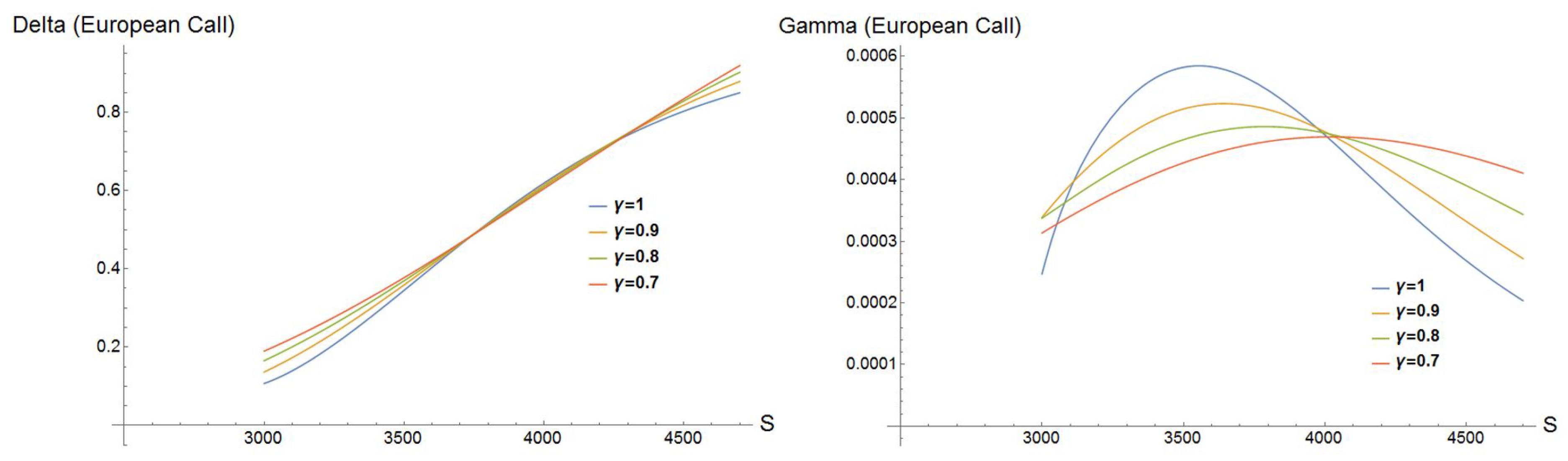
In the left figure, we plot the evolution of the Delta of an European call option as a function of S for various values of . We observe that, as expected from (83), the At-The-Money (ATM) call price is approximately equal to for any , and moreover, the Delta value is the same on a wide range of prices around , independently of . The situation is very different on the right figure (plot of the Gamma of the European call option (93)), where sensitivities vary greatly in dependence of . To produce the figures, the following values of parameters were used: , , , , .
Figure 1.
In the left figure, we plot the evolution of the Delta of an European call option as a function of S for various values of . We observe that, as expected from (83), the At-The-Money (ATM) call price is approximately equal to for any , and moreover, the Delta value is the same on a wide range of prices around , independently of . The situation is very different on the right figure (plot of the Gamma of the European call option (93)), where sensitivities vary greatly in dependence of . To produce the figures, the following values of parameters were used: , , , , .

Figure 2.
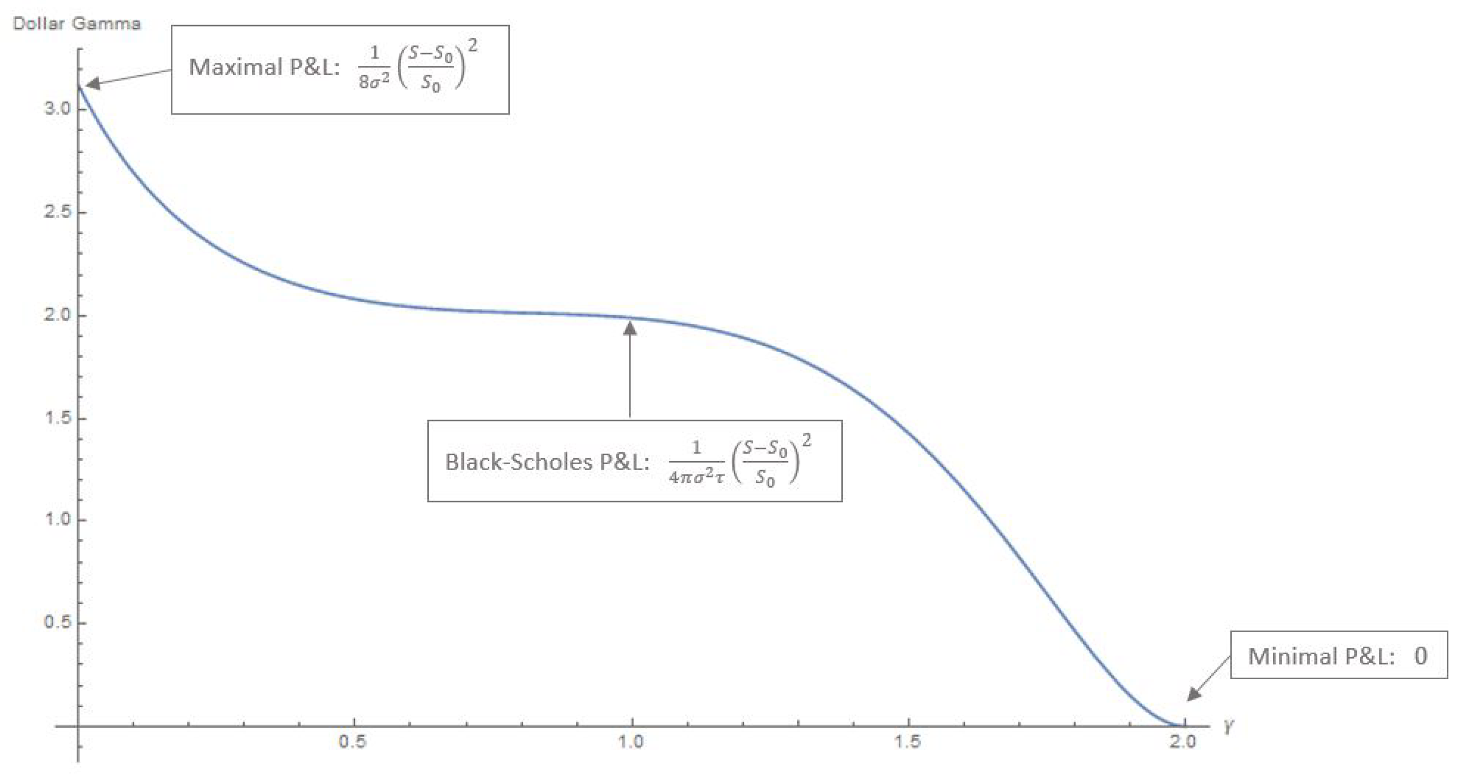
The dollar Gamma for the time-fractional diffusion model (,) maximizes the P&L when and offsets the impact of maturity at extremal values (, ). The graph of the Dollar Gamma possesses an inflection point at the point (the Black-Scholes model). To produce the figure, the following values of parameters were used: , .
Figure 2.
The dollar Gamma for the time-fractional diffusion model (,) maximizes the P&L when and offsets the impact of maturity at extremal values (, ). The graph of the Dollar Gamma possesses an inflection point at the point (the Black-Scholes model). To produce the figure, the following values of parameters were used: , .

© 2019 by the authors. Licensee MDPI, Basel, Switzerland. This article is an open access article distributed under the terms and conditions of the Creative Commons Attribution (CC BY) license (http://creativecommons.org/licenses/by/4.0/).
Share and Cite
MDPI and ACS Style
Aguilar, J.-P.; Korbel, J.; Luchko, Y. Applications of the Fractional Diffusion Equation to Option Pricing and Risk Calculations. Mathematics 2019, 7, 796. https://0-doi-org.brum.beds.ac.uk/10.3390/math7090796
AMA Style
Aguilar J-P, Korbel J, Luchko Y. Applications of the Fractional Diffusion Equation to Option Pricing and Risk Calculations. Mathematics. 2019; 7(9):796. https://0-doi-org.brum.beds.ac.uk/10.3390/math7090796
Chicago/Turabian StyleAguilar, Jean-Philippe, Jan Korbel, and Yuri Luchko. 2019. "Applications of the Fractional Diffusion Equation to Option Pricing and Risk Calculations" Mathematics 7, no. 9: 796. https://0-doi-org.brum.beds.ac.uk/10.3390/math7090796
Note that from the first issue of 2016, this journal uses article numbers instead of page numbers. See further details here.