Multi-Attribute Decision-Making Methods as a Part of Mathematical Optimization

Department of Information Technologies, Vilnius Gediminas Technical University, 10223 Vilnius, Lithuania
Mathematics 2019, 7(10), 915; https://0-doi-org.brum.beds.ac.uk/10.3390/math7100915
Submission received: 21 August 2019
/
Revised: 13 September 2019
/
Accepted: 26 September 2019
/
Published: 2 October 2019
(This article belongs to the Special Issue Optimization for Decision Making)
Abstract
:Optimization problems are relevant to various areas of human activity. In different cases, the problems are solved by applying appropriate optimization methods. A range of optimization problems has resulted in a number of different methods and algorithms for reaching solutions. One of the problems deals with the decision-making area, which is an optimal option selected from several options of comparison. Multi-Attribute Decision-Making (MADM) methods are widely applied for making the optimal solution, selecting a single option or ranking choices from the most to the least appropriate. This paper is aimed at providing MADM methods as a component of mathematics-based optimization. The theoretical part of the paper presents evaluation criteria of methods as the objective functions. To illustrate the idea, some of the most frequently used methods in practice—Simple Additive Weighting (SAW), Technique for Order of Preference by Similarity to Ideal Solution (TOPSIS), Complex Proportional Assessment Method (COPRAS), Multi-Objective Optimization by Ratio Analysis (MOORA) and Preference Ranking Organization Method for Enrichment Evaluation (PROMETHEE)—were chosen. These methods use a finite number of explicitly given alternatives. The research literature does not propose the best or most appropriate MADM method for dealing with a specific task. Thus, several techniques are frequently applied in parallel to make the right decision. Each method differs in the data processing, and therefore the results of MADM methods are obtained on different scales. The practical part of this paper demonstrates how to combine the results of several applied methods into a single value. This paper proposes a new approach for evaluating that involves merging the results of all applied MADM methods into a single value, taking into account the suitability of the methods for the task to be solved. Taken as a basis is the fact that if a method is more stable to a minor data change, the greater importance (weight) it has for the merged result. This paper proposes an algorithm for determining the stability of MADM methods by applying the statistical simulation method using a sequence of random numbers from the given distribution. This paper shows the different approaches to normalizing the results of MADM methods. For arranging negative values and making the scales of the results of the methods equal, Weitendorf’s linear normalization and classical and author-proposed transformation techniques have been illustrated in this paper.
Keywords:
optimization; decision-making; MADM; SAW; COPRAS; TOPSIS; PROMETHEE; MOORA; normalization; stability1. Introduction
In a specific activity, a person consciously and intuitively seeks to find the best solutions to emerging problems or tasks. The action of making the best or most effective use of a situation or resource is called optimization. The Simple Additive Weighting (SAW), Technique for Order of Preference by Similarity to Ideal Solution (TOPSIS), Complex Proportional Assessment Method (COPRAS), Multi-Objective Optimization by Ratio Analysis (MOORA) and Preference Ranking Organization Method for Enrichment Evaluation (PROMETHEE) methods applied in this paper have been described in different research papers as Multiple Criteria Decision Making (MCDM) [1,2,3,4,5,6], Multiple Attribute Decision Making (MADM) [7,8,9], Multiple Criteria Decision Analysis (MCDA) [10] or Multi-Attribute Decision Analysis (MADA) [11], and Multi-Criteria Analysis (MCA) [12,13]. Since this work is focused on decision-making and the number of alternatives are explicitly given and finite, the name MADM will be used to define the above-listed methods.
MADM methods are aimed at identifying the most satisfactory of several comparative alternatives or at ranking options according to their relevance in terms of the evaluated objective [14]. The methods are used for selecting the most satisfactory alternative/solution provided that there is no such alternative for which all criteria values are the best.
To solve an optimization problem with classical optimization methods, the function of its objective is fixed, establishing the set of objects to be optimized or the allowable area to be determined. The minimum or maximum values of the function are sought depending on the purpose of the problem being solved. The theoretical part of this work presents MADM methods as a component of mathematical optimization methods, and evaluation criteria for SAW, TOPSIS, COPRAS, MOORA and PROMETHEE methods appear as objective functions, which is a new form of presenting and interpreting methods. To illustrate the idea of this publication, some of the most widely applied MADM methods have been selected. The presented methodology can be transferred to other methods as well.
The judging matrix and the vector of criterion weights are the components of most of MADM methods. The judging matrix covers statistical data or the values of expert evaluation according to the criteria defining the objective [14]. Since the impact of criteria on the outcome of the problem to be solved is different, the significance (weights) of criteria is determined [15]. Criterion weights can be clarified directly or by employing certain weighting methods. The main idea of most of the used MADM methods is merging criterion values and their weights into a single evaluation characteristic (i.e., the summarized criterion of the method). Data on MADM methods are static, and their values do not vary in the problem-solving process.
Most of the assignments solved by people include problems that do not have sufficient numerical data or problems where the investigated objects are impossible to measure. In such cases, the judgment matrix is supplemented by the data obtained from the expert evaluation. Particular focus is switched to selecting experts in a particular field, considering their characteristics related to professional competence, work experience, scientific degree, research activity and the ability to address specific issues in the field given. MADM methods operate in numerical values, although the criteria themselves can be both quantitative and qualitative. The qualitative meanings of criteria, in some cases, facilitate expert evaluation that can be individual when the expert expresses individual opinions independently of other experts or shared and accepted in a group of professionals.
The research literature does not propose the best or most appropriate MADM method for dealing with a specific problem. This question is relevant, and thus there are many research papers focused on determining the stability of the method on the basis that any mathematical model or method can be applied in practice in the case that they remain stable with respect to the applied parameters [16]. A mathematical model is considered to be stable if a small change in the results is consistent with minor variations in the parameters for the model. Multiple MADM methods are applied in most complex decision-making tasks to ensure the accuracy of the final result. In the cases when several MADM methods are used for evaluation, it becomes unclear what results of which method are reliable. This paper proposes a new approach that helps the expert make the right decision. The core of the suggested approach is to apply several MADM methods and to determine the suitability/impact of the employed MADM methods on the problem solved (i.e., to clarify the stability of the method). The final result consists of the estimates of several methods taking into account the weight of the effect of each method.
The paper verifies the stability of multi-criteria methods when slightly changing data in the matrix of the initial solution (i.e., expert evaluations and weights of the vector, fixing recurrence frequency of the best alternative to the initial data). Previous papers of the author considered that the higher the number of imitations, the more accurate the evaluation of the stability of the multi-criteria method (i.e., the range of the varying result decreased). A sufficient number of recurrences was established when the result of evaluating MADM stability remained almost unchanged, because 105 times could be treated as an adequate number of estimations [17].
The practical part of the paper combines the results of several MADM methods into a single outcome and shows a few ways to normalize results obtained using MADM methods of different scales.
2. Literature Review
Analytical mathematical optimization problems were solved in as early as the 17th century. The first solution proposed investigating the problem of finding the minimum/maximum and was described by P. Fermat (XVII). Newton developed the method of fluxions. The technique was rediscovered and published in the paper “New Method for the Greatest and the Least” by G. W. Leibniz in 1684. Further, efforts exerted by Euler and Lagrange led to working out solutions to extreme tasks. In 1824, Fourier created the first algorithm for solving linear arithmetic constraints [18]. This algorithm made further advances in the field, such as the main duality theorem, the Farkas lemma, the Motzkin transfer theorem and others [19]. The traditionally employed model of optimization includes linear programming, sequential quadratic programming, nonlinear programming, and dynamic programming [20]. In 1939, the first formulation of the linear programming problem and the method for solving this problem were proposed by Leonid Kantorovich. In 1947, Danzig created the simplex method that was effectively used to solve linear programming problems [21]. Derivative-based stochastic optimization began with a seminal paper by Robbins and Monro (1951) that launched the entire field [22]. Richard Bellman developed the dynamic programming method in the 1950s [23].
Decision-making methods based on optimality were introduced by Pareto in 1896 and applied to a wide range of problems. The Multi-Objective Evolutionary Algorithm (MOEA) [24] is used to find the optimal Pareto solutions for specific problems [25]. Keeney and Raiffa [26] and Fishburn [27] introduced the Multi-Attribute Value Theory (MAVT), the Multi-Attribute Value Analysis (MAVA) and Multi-Attribute Utility Theory (MAUT) methods. Data envelopment analysis (DEA), introduced by Charnes et al., is a linear programming method for measuring the efficiency of multiple decision-making units by analysing the problems of multiple inputs and outputs [28].
Multiple criteria decision-making methods evolved from operations research theory by solving problems such as the development of computational and mathematical tools to support the subjective assessment of performance criteria by decision-makers [29]. MADM, as a discipline, has a relatively short history of approximately 30 years. Its role has increased significantly in different application areas along with the development of new methods and improved old methods in particular.
A work by Hwang and Yoon presented a plethora of methods for solving MADM problems [7]: Methods for Cardinal Preference of Attribute over Linear Assignment method [30], Simple Additive Weighting (SAW) method [31], Hierarchical Additive Weighting method, ELECTRE method, and Technique for Order of Preference by Similarity to Ideal Solution (TOPSIS) [7]. The most familiar and commonly used is the SAW method reflecting the idea of multi-criteria methods—merging criterion values and their weights into a single value [32].
Peng and Wang proposed the concept of hesitant uncertain linguistic Z-numbers (HULZNs) and presented the Multi-Criteria Group Decision-Making (MCGDM) method by integrating power operators employing the Vlse Kriterijumska Optimizacija I Kompromisno Resenje (VIKOR) [5] model. Peng and Wang merged the Multi-Objective Optimization by Ratio Analysis plus the Full Multiplicative From (MULTIMOORA) and power aggregation operators in order to create a comprehensive decision model for MCGDM problems with Z-numbers [33]. Outranking ELECTRE [34] and PROMETHEE [35] methods were described in the publication on multiple criteria decision analysis by Belton and Stewart in 2001 [10]. Opricovic and Tzeng conducted a comparative analysis of VIKOR and TOPSIS methods in 2004 [5,36].
New methods have recently emerged that are actively used in different fields of science: Weighted Aggregated Sum Product Assessment (WASPAS) [37], Complex Proportional Assessment Method (COPRAS) [38], Multi-Objective Optimization by Ratio Analysis (MOORA) [39], COPRAS grey (COPRAS-G), fuzzy additive ratio assessment (ARAS-F) [40], ARAS grey (ARAS-G) and MULTIMOORA (MOORA plus the full multiplicative form) [41,42], KEmeny Median Indicator Ranks Accordance (KEMIRA) [43], ARAS [44], and newest extensions of the ELECTRE [45] and PROMETHEE [46,47] methods. The examples of partial aggregation methods include Step-Wise Weight Assessment Ratio Analysis (SWARA) [48] and factor relationship (FARE).
Criterion weights are one of the components of MCMD methods and therefore have a strong impact on the final result [15]. For defining criterion weights, subjective evaluation is the most frequently applied technique when experts examine the significance of criteria, although objective and generalized estimates are known [49]. Weights can be set directly or using weighting methods such as Analytic Hierarchy Process (AHP) [50,51], Fuzzy Analytic Hierarchy Process (FAHP) [52,53], SWARA [54], Criterion Impact LOSs (CILOS) [55], Integrated Determination of Objective Criteria Weights (IDOCRIW) [14,56], etc. Recalculation of the weights of criteria under the Bayes theorem is proposed in the paper [56]. Regardless of the method, the principles of evaluation remain to take the position that the weight of the most important criterion is the highest. It was agreed that the sum of all weights should be equal to 1 [1]. Any measurement scale may be used for evaluations.
Based on a study by Sabaei et al., the most common decision management methods used in Scopus database publications are AHP, ELECTRE, and PROMETHEE [57]. The early 1990s witnessed the shift of focus toward methods that consider indifference and ensure the transparency of analysis processes [58]. An analogous study conducted by Mardani et al. aimed at determining the popularity of decision-making methods. The results showed that hybrid MADM and fuzzy MADM approaches (27.92%) were used more often than other methods. The most commonly used methods are AHP and fuzzy AHP [59] (24.87%), ELECTRE, fuzzy ELECTRE [60], MCDA and MCA (12.69%), and TOPSIS, fuzzy TOPSIS [61], PROMETHEE and fuzzy PROMETHEE [62] (5.08%) [1].
Mardani et al. carried out research and published the obtained material in the paper “Multiple Criteria Decision-Making Techniques and Their Applications,” (i.e., a literature review for the period from 2000 to 2014 [2]). Another paper by Mardani et al. reviewed decision-making methods from the field of energy management for the period 1995–2015 [1].
The concept of sensitivity analysis in decision theory means the effective use and implementation of quantitative decision models, the purpose of which is to assess the stability of an optimal solution under changes in parameters, the impact of the lack of controllability of specific parameters and the need for the precise estimation of parameter values [63]. The first significant works on sensitivity analysis in the field of decision-making were done by Evans [63], who formulated the concepts of sensitivity analysis in linear programming to develop a formal approach applicable to classical decision-theoretic problems [64] and presented two simple computational procedures for sensitivity analysis of additive multi-attribute value models that yielded variations in attribute weights. Insua [65] developed a conceptual framework for sensitivity analysis in discrete multi-criteria decision-making, which allowed simultaneous variations in judgmental data and applied to many paradigms for decision analysis. Janssen [66] discussed the sensitivity of the rankings of alternatives to the overall uncertainty in scores, and priorities were analyzed using the Monte Carlo approach. Butler [67] presented a simulation approach allowing simultaneous changes in the weights and generating results that could be easily analyzed to provide insights into multi-criteria model recommendations statistically.
Wolters and Mareschal [68] proposed three novel types of sensitivity analysis focused on and elaborated for the PROMETHEE methods. Masuda [69] studied the sensitivity problems of the AHP method. In his work, he concentrated on how changes in the entire columns of the decision-making matrix might affect the values of the composite priorities of alternatives. Triantaphyllou [70] presented a methodology for performing a sensitivity analysis of the weights of decision criteria and identifying the performance values of the alternatives expressed in terms of decision criteria. The estimation of the effect/impact of uncertainty in the SAW method was performed by Podvezko [71], who determined the points of varying ranges of criterion weights of the investigated process, evaluated compatibility level and stability of expert opinions and assessed the effect of uncertainty on ranking comparable objects employing the imitation method. The impact of varying weights on the final result in the SAW method was studied by Zavadskas [72] and Memariani [73]. The influence of the elements of the decision matrix on the final ranking result was analyzed by Alinezhad [74]. The effect of the importance of criterion weights on the results of the TOPSIS method was studied by Yu [75] and Alinezhada [76]. Misra focused on a comparison of AHP, Decision-Making Trial and Evaluation Laboratory (DEMATEL), COPRAS, and TOPSIS methods [77]. Podvezko [32] compared SAW, TOPSIS and COPRAS methods. Moghassem [78] increased and decreased all criterion weights by 5%, 10%, 15%, and 20% in analyzing the sensitivity of TOPSIS and VIKOR. Hsu conducted the sensitivity analysis of TOPSIS by increasing and decreasing the top three weights by 10% [79].
3. MADM Methods as a Component of Mathematics-Based Optimization Techniques
To formulate the optimization problem, the paper presents a set of optimized elements and the measure of goodness of its elements (quality estimates).
The optimization problem takes the form of
where is the objective function or criterion; D is the set or permissible area of the optimized objects; and is the minimum or maximum value of function .
The literature provides a number of different classifications of optimization problems. Typically, specific decision-making methods are created for each category of problems according to the characteristics of that particular class. Weights do not vary in SAW, TOPSIS, COPRAS, MOORA and PROMETHEE methods. Weights are determined using subjective or objective weighting methods. The number of comparable alternatives is finite in these methods.
MADM methods can be presented as a mathematical optimization problem as follows:
where ν is the number of the MADM method. The merit of alternatives is evaluated according to criteria , and the values are defined as . The influence of criteria on the evaluation result is different, and therefore the vector , , of the weights of criteria is determined, thus defining the importance of criteria.
3.1. SAW (Simple Additive Weighting) Method (ν = 1)
When the values of criteria are multi-dimensional, they are transformed. The values of the maximized criteria are calculated according to the formula:
Then, the highest value of is equal to 1. The value of minimized criteria is correspondingly calculated according to the formula:
Then, the lowest value of is equal to 1. For standard criteria, the principle of simple linear scalarization is applied.
3.2. TOPSIS (Technique for Order of Preference by Similarity to Ideal Solution) Method (ν = 2)
The method refers to vector data normalization:
where is the normalized value of the jth criterion for the ith alternative.
The vector of the best value and the worst value of criteria (ideal alternative) are calculated as
where is a set of indices of the maximized criteria, is a set of indices of the minimized criteria, and is the worst (best) value of the jth criterion.
The basic principle of the method is to find an alternative at the shortest overall distance from the best values of criteria and the maximum distance from the worst values. The method does not require the rearrangement of the minimized (maximized) criteria to the maximized (minimized) ones.
3.3. PROMETHEE (Preference Ranking Organization Method for Enrichment Evaluation) Method (ν = 3)
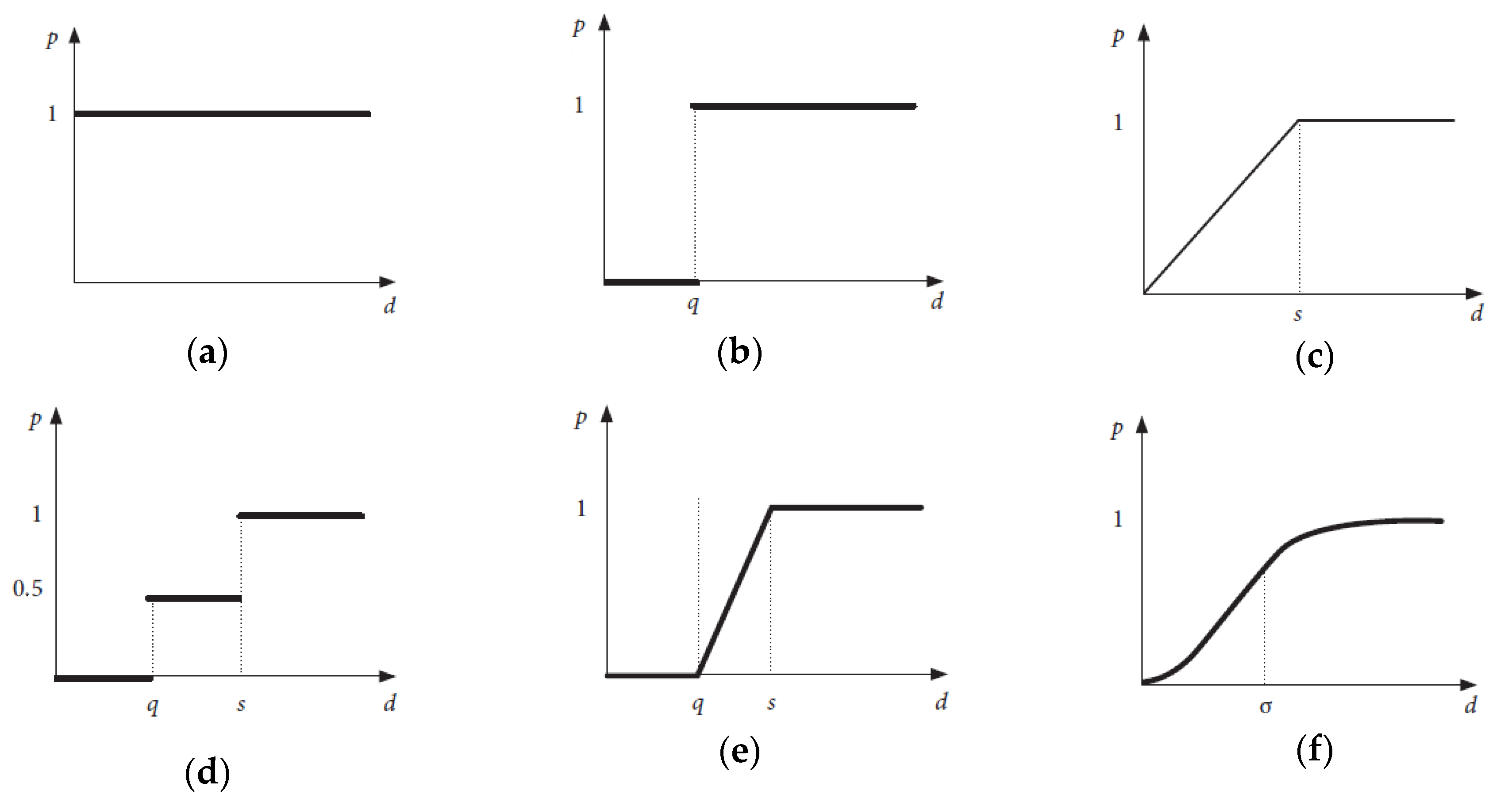
The PROMETHEE method uses the basic ideas of other methods like combining the values of weights and normalized criteria into a single estimate (SAW method) and the pairwise comparison of criteria (AHP method). Instead of the normalized criteria values, the value of the priority function , is used, and all possible pairs of alternatives for each of the criteria are compared with each other. A higher value of corresponds to a better alternative; if the difference is lower than the established critical value , then = 0. If the maximum limit for the values of criteria, then .
The priority function of the usual criterion is equal to
The function chart is shown in Figure 1a.
The priority function of the U-shape criterion is equal to
The function chart is shown in Figure 1b.
The priority function of the V-shape criterion (linear priority) is equal to
The function chart is shown in Figure 1c.
The priority function of the level criterion is equal to
The function chart is shown in Figure 1d.
The priority function of the V-shape with indifference criterion is equal to
The function chart is shown in Figure 1e.
The priority function of the Gaussian criterion is equal to
The function chart is shown in Figure 1f.
As mentioned above, PROMETHEE, similarly to the other multi-criteria decision methods, applies the idea of the SAW method instead of the normalized values of criteria and uses the values of the functions of specifically selected priorities, where the argument is the difference between the values of the criterion.
3.4. COPRAS (Complex Proportional Assessment) Method (ν = 4)
3.5. MOORA (Multi-Objective Optimization on the Basis of Ratio Analysis) Method (ν = 5)
For the value of , vector normalization according to Equation (8) is applied. The initial version of the MOORA method did not take into account the importance of the criteria expressed in weights. The method calculation principle is the sum of the values of the minimized normalized criteria (from to ) subtracted from the sum of the maximized normalized alternative criteria (from to ). For developing the MOORA method, Brauers started using the weights of criteria [39]. The improved MOORA method is applied for calculations.
The presented methods have been selected as some of those most frequently applied in practice. Similarly, other familiar criteria such as VIKOR, ELECTRE, and others for evaluating the MADM method can be presented as objective functions.
4. Experimental Application of the Methodology Merging MADM Methods
The application of a few MADM methods may result in ranking the scale of evaluation results and reported findings, which is not a clear case of what decision should be made. Each method has an individual theoretical basis and logic, and therefore results in differences.
This chapter describes the methodology for merging the results of MADM methods and presents its practical application. The methodology proposes making calculations using several MADM methods and thus merging their results according to the importance of the method for the problem solved into a single value. SAW, COPRAS, TOPSIS, PROMETHEE and MOORA methods are used in the calculations.
To sum up the results of different methods into the single value, normalizing result data beforehand is required. Linear, classical, vector, logarithmic and other normalization techniques are known. Unlike other methods, the results received applying PROMETHEE are both positive and negative numbers. To transform the results of the PROMETHEE method and other MADM techniques to the uniform scale, PROMETHEE result data must be converted into positive values.
4.1. Methodology for Merging the Results of MADM Methods
The weight, representing the importance of the MADM method, is defined as . The result of the stability of a separate method is defined as and is expressed in percentage.
The weights of methods are normalized in the following way:
The best alternative is established as
where is the normalized result of the th MADM method of the ith alternative.
To merge the results of different methods into a single value, normalizing data on the obtained results is required beforehand. Linear, classical, vector, logarithmic and other normalization techniques are known. Unlike other methods, the results received applying PROMETHEE are both positive and negative numbers. To transform the results of the PROMETHEE and other MADM methods to the uniform scale, first, PROMETHEE result data must be converted into positive values.
For handling negative values and making the scales of the results of other methods equal, Wietendorf’s [82] linear normalization rearranging data in the range of [0, 1] is suitable:
where is the normalized result of the method and , x is the initial obtained result of the method, is the lowest value of the results of methods, and is the highest value of the results of methods.
Another method for making data on MADM results equal in order to employ classical normalization [83] is as follows:
Thus, the results of the PROMETHEE method are transformed into positive numbers beforehand. The transformed value of the evaluation result takes the form of , i = 1, …, n. The results of obtained applying the PROMETHEE method are sorted in ascending order. The lowest result of the transformed method is equal to . Other transformed values are calculated as follows:
4.2. Algorithm for Defining MADM Stability
Any mathematical model or method can be applied in practice provided it is stable in terms of the applied parameters. The stability of MADM is verified by employing the statistical simulation method using a sequence of random numbers from the given distribution.
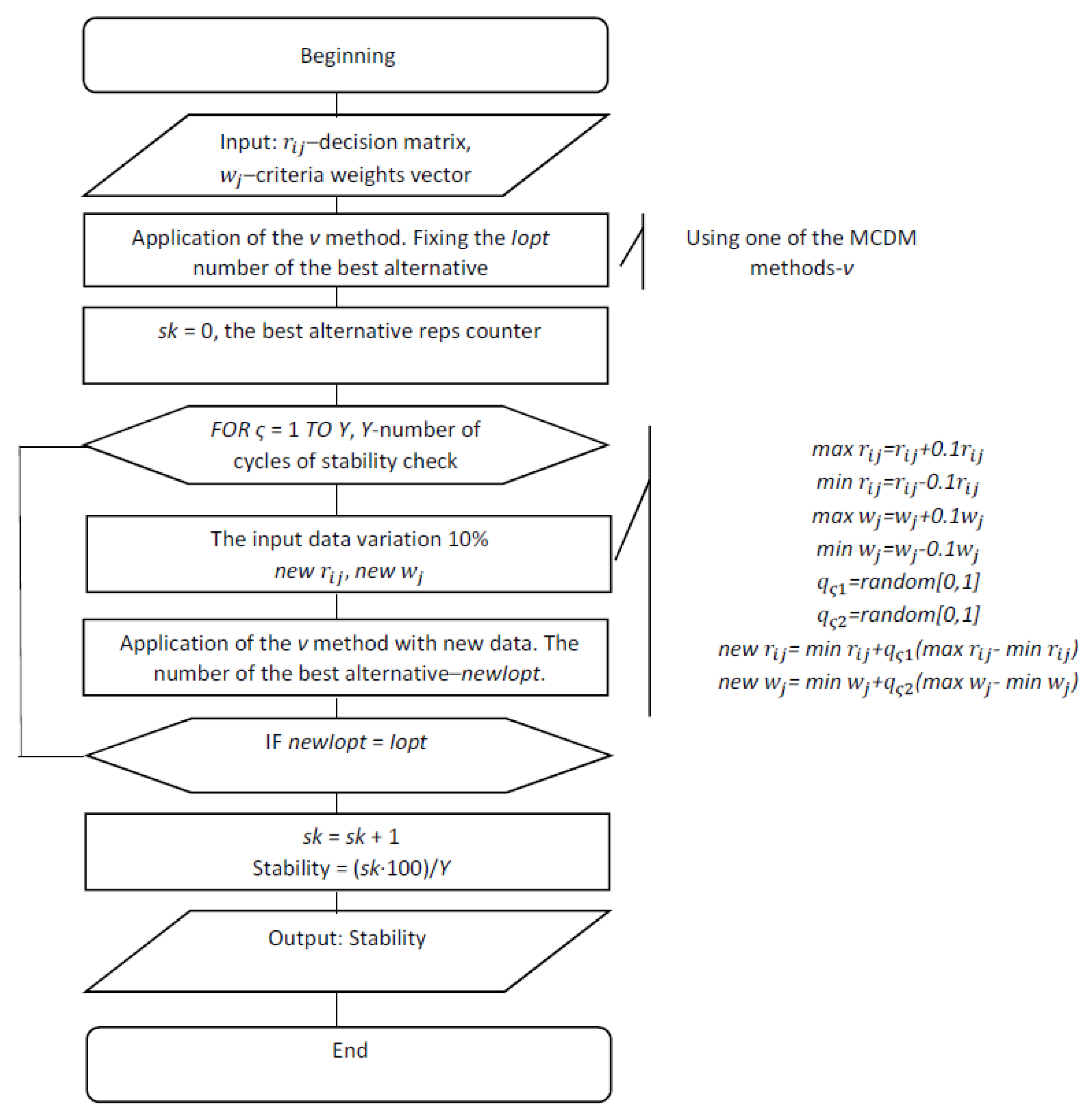
The algorithm for evaluating the stability of the MADM method is presented in Figure 2.
MADM method determines the best alternative i of the initial data and fixes the number of this alternative Iopt. Verifying the stability of multi-criteria methods brings slight changes in vector data in the initial judging matrix (i.e., expert evaluations and weights ). The calculation is made with the newly received values and using the MADM method, thus determining the number of the best alternative newIopt. The counter sk captures the amount of newIopt recurrence with the initial Iopt. As mentioned in the introduction, a sufficient number of cycles to evaluate the stability of the method to the nearest 0.1 was selected with Y = 105.
The stability coefficient that fixes the frequency of the recurrence of the best initial alternative is calculated by changing preliminary data. The method is more important for the result of the problem when the stability coefficient is higher.
When no information on the distribution of parameters for MADM methods is available, the uniform distribution is used for generating random values of from the range []:
where ϵ [0, 1].
The random values of alternate estimates and criterion weights are generated by slightly changing initial data and by 10% when :
The variation limits [] of alternative estimates are determined as
Accordingly, the variation limits [] of criterion weights are equal to
By applying the algorithm for verifying the stability of the MADM method (Figure 2), the stability of all multi-criteria decision-making methods described in this paper is checked. The higher the frequency of the reoccurrence of the best alternative, the more stable the method. The proposed method considers the uncertainty of data on expert evaluation and therefore decreases the level of the subjectivity of the conducted evaluation. The evaluation carried out by applying multiple MADM methods allows selecting the result of the most stable method or merging the results of several methods into a single value.
4.3. Experimental Application of Merging the Results of MADM Methods
To illustrate the application of the method described in the paper, an example in which the estimates of alternatives differ slightly from each other has been chosen. The experts assessed the quality of the course units taught according to six criteria [17]. The descriptions of criteria, as well as the estimates of weights and course units, are given in Table 1. The mean of alternative estimates (i.e., course units), is in the range of [9.03, 9.34].
Regarding the initial data (Table 1), the calculation has been conducted by applying the SAW (Equation (3)), TOPSIS (Equation (7)), MOORA (Equation (18)), COPRAS (Equation (17)) and PROMETHEE (Equation (10)) methods. Since all criteria are maximized in the problem solved (Table 1), the calculation of the SAW and COPRAS methods coincides [34]. Thus, only the SAW method will be mentioned below in the paper. The calculations of the PROMETHEE method used the function chart of the priority of the V-shape with indifference criterion (Equation (15)) with parameters q {0.25; 1.75; 0.3; 0.25; 0.2} and {1.2; 2; 0.6; 1.5; 0.75}. The parameters and were not changed, testing the stability of the PROMETHEE method.
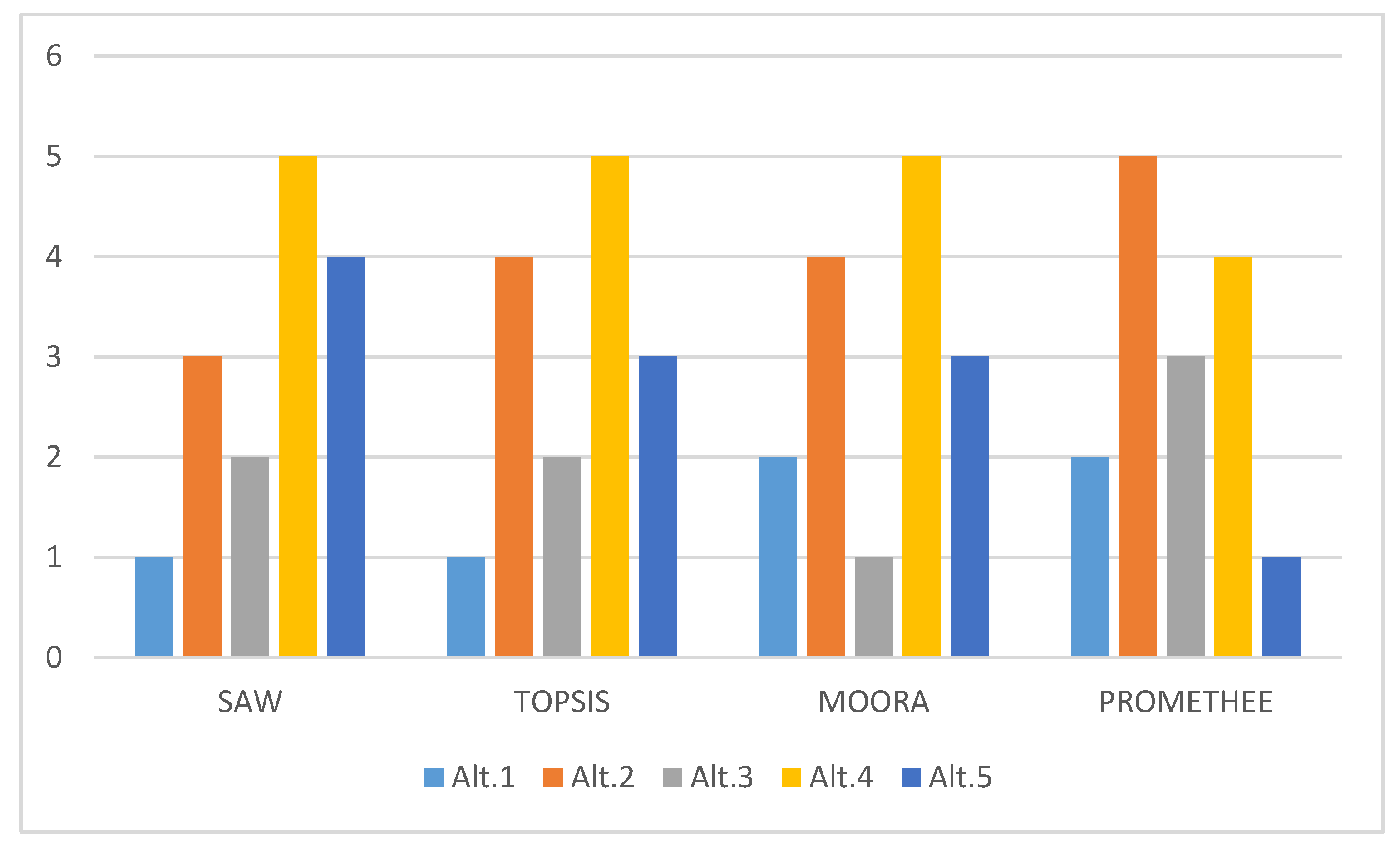
The final ranked results are presented in Figure 3. The best alternative is ranked 1, whereas the worst-rated alternative takes 5. Calculations revealed that the results of the methods differ: SAW method results {0.2022; 0.2001; 0.2020; 0.1958; 0.1999}, TOPSIS {0.6029; 0.5272; 0.6004; 0.3640; 0.5413; 3}, MOORA {4.2080; 4.1196; 4.2103; 3.9963; 4.1316}, PROMETHEE {0.2127; −0.3252; 0.0889; −0.2309; 0.2544} [84]. Therefore, it is not possible to unambiguously identify the best course unit from the results obtained.
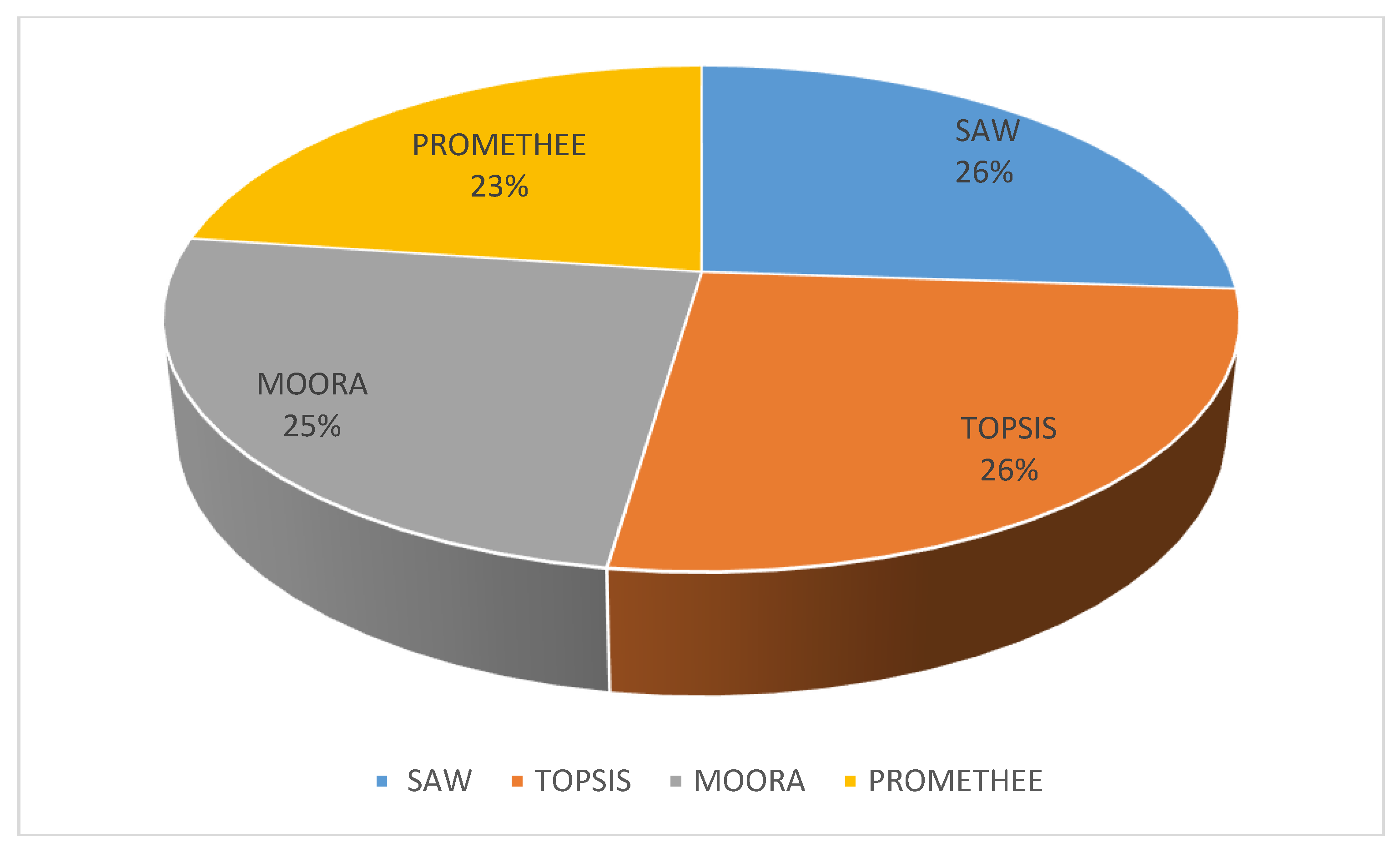
According to the algorithm described above, the stability of the following methods has been determined: SAW 30.7%, TOPSIS 30.9%, MOORA 29.3% and PROMETHEE 26.8%.
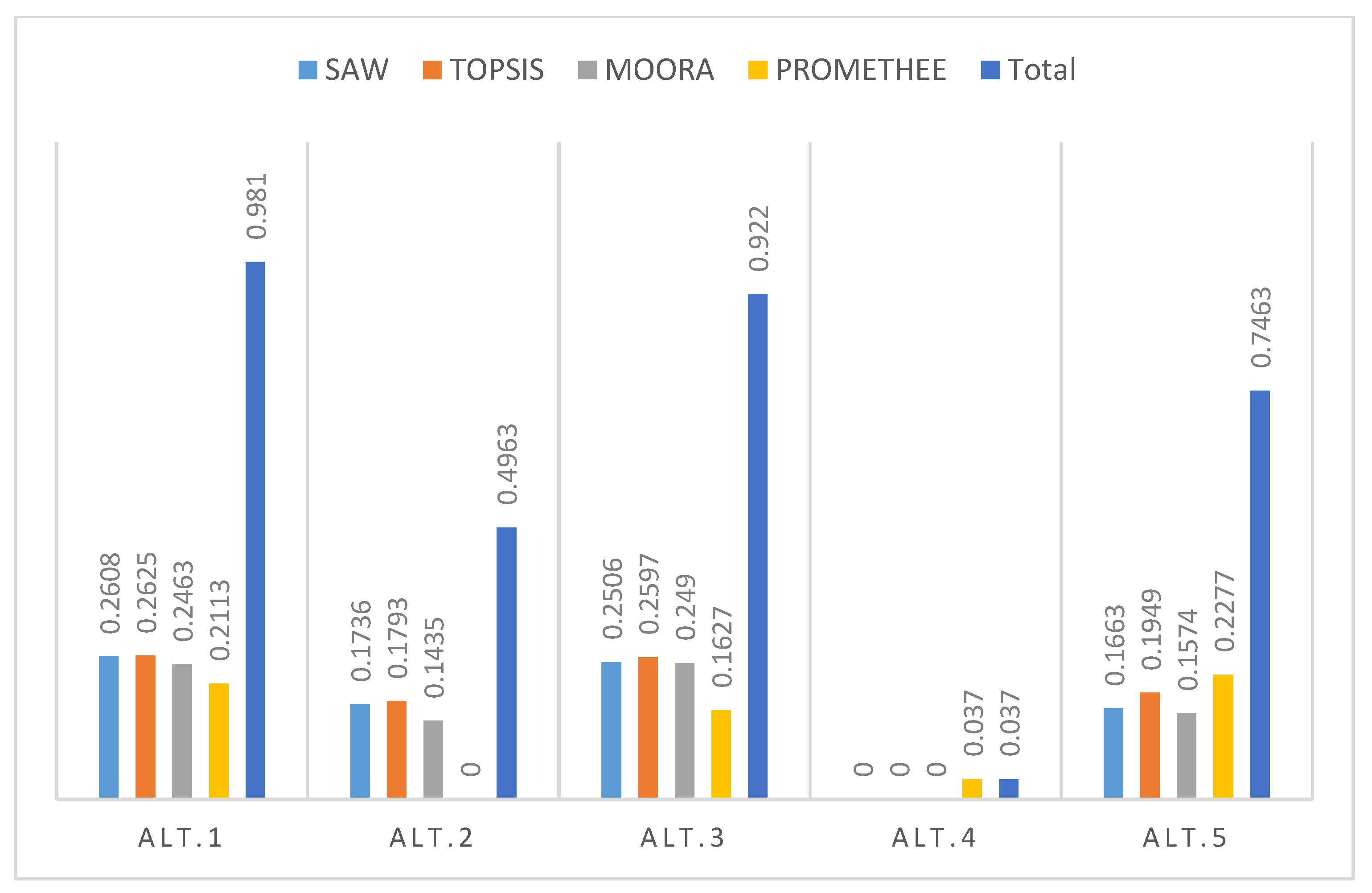
The stability of all methods is low due to the similarity of the initial data. Even small variations in the initial data have changed ranking of the best alternative. Having applied Equation (19), the weights of methods are calculated: ΩSAW = 0.2608, ΩTOPSIS = 0.2625, ΩMOORA = 0.249, ΩPROMETHEE = 0.2277 (Figure 4). The weights of the methods are slightly different, and the most stable is the TOPSIS method.
In order to merge the results of all methods, their estimates need to be unified. Thus, the MADM results are normalized in the range of [0, 1] (Table 2). Wietendorf’s [82] linear normalization is suitable for the results of different scales as well as for the negative values of the PROMETHEE method.
Equation (20) is applied in summing up the estimates of the normalized methods considering their weights. The numerical results are presented in Figure 5. A comparison of the obtained results (Figure 5) with data provided in Table 1 shows changes in the findings. The weights of criteria had a significant impact on the result. Compared to the ranked results employing all methods, the merged MADM result matched with that determined by applying the TOPSIS method. The latter method had a higher weight (i.e., importance), in the problem solved.
Table 2 shows that Wietendorf’s (Equation (21)) linear normalization has a disadvantage (i.e., zero estimates of alternatives). The weight of the method does not affect the worst-rated alternative as its result is normalized to the zero value.
When the results of two worst-rated alternative methods slightly differ from each other using different normalization, the result may change. Thus, no similar problems are encountered in finding the best alternative.
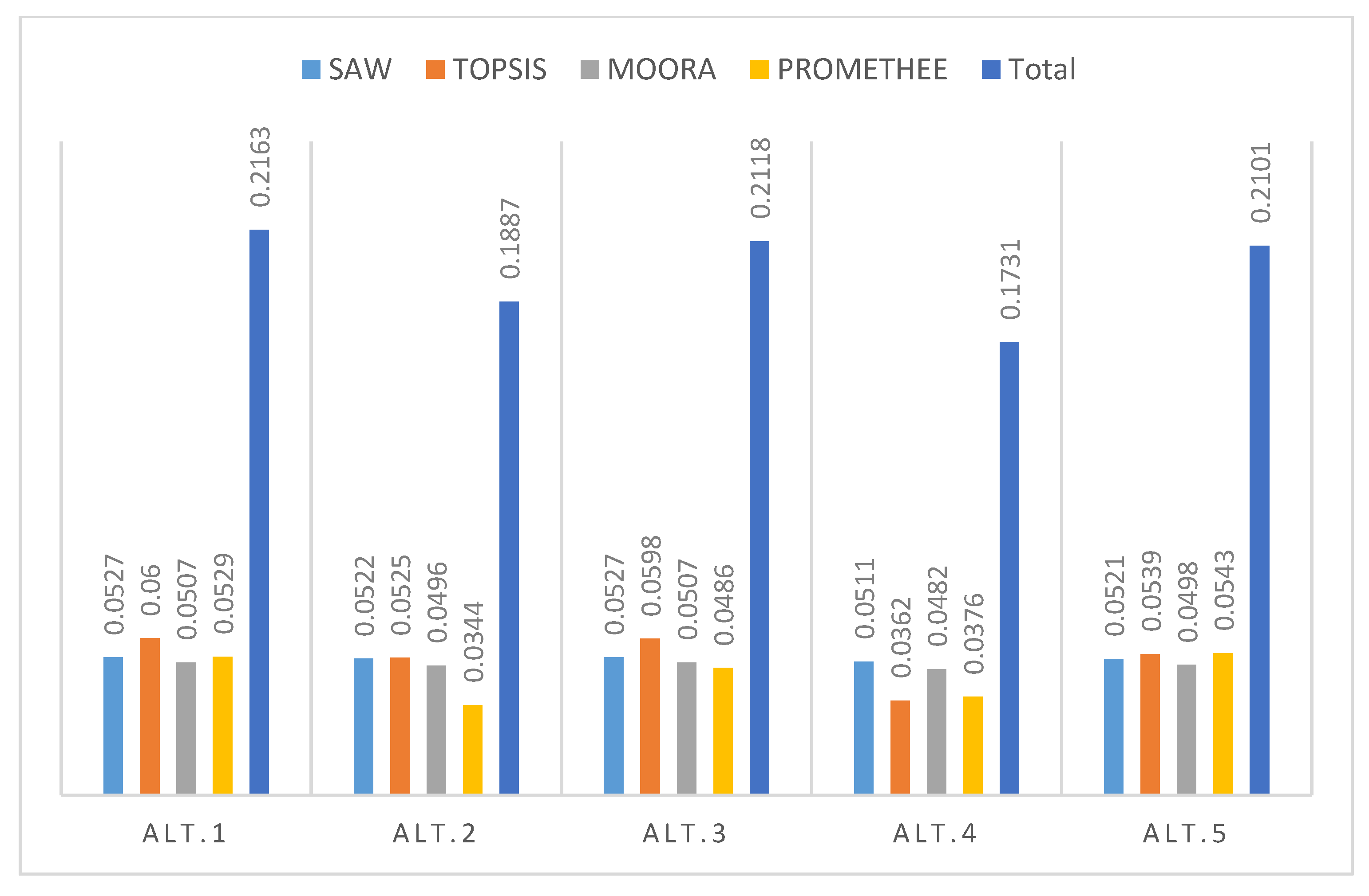
Another calculation method (i.e., technique for making values equal), involves classical normalization (Equation (22)) and pre-arranging the results of the PROMETHEE method using Equation (23). The transformed positive results of the PROMETHEE method are 1.5379, 1, 1.4141, 1.0943, and 1.5795. Table 3 shows the re-estimation of the methods using classical normalization [84]. The results of the MADM methods merged using Equation (20) are shown in Figure 6.
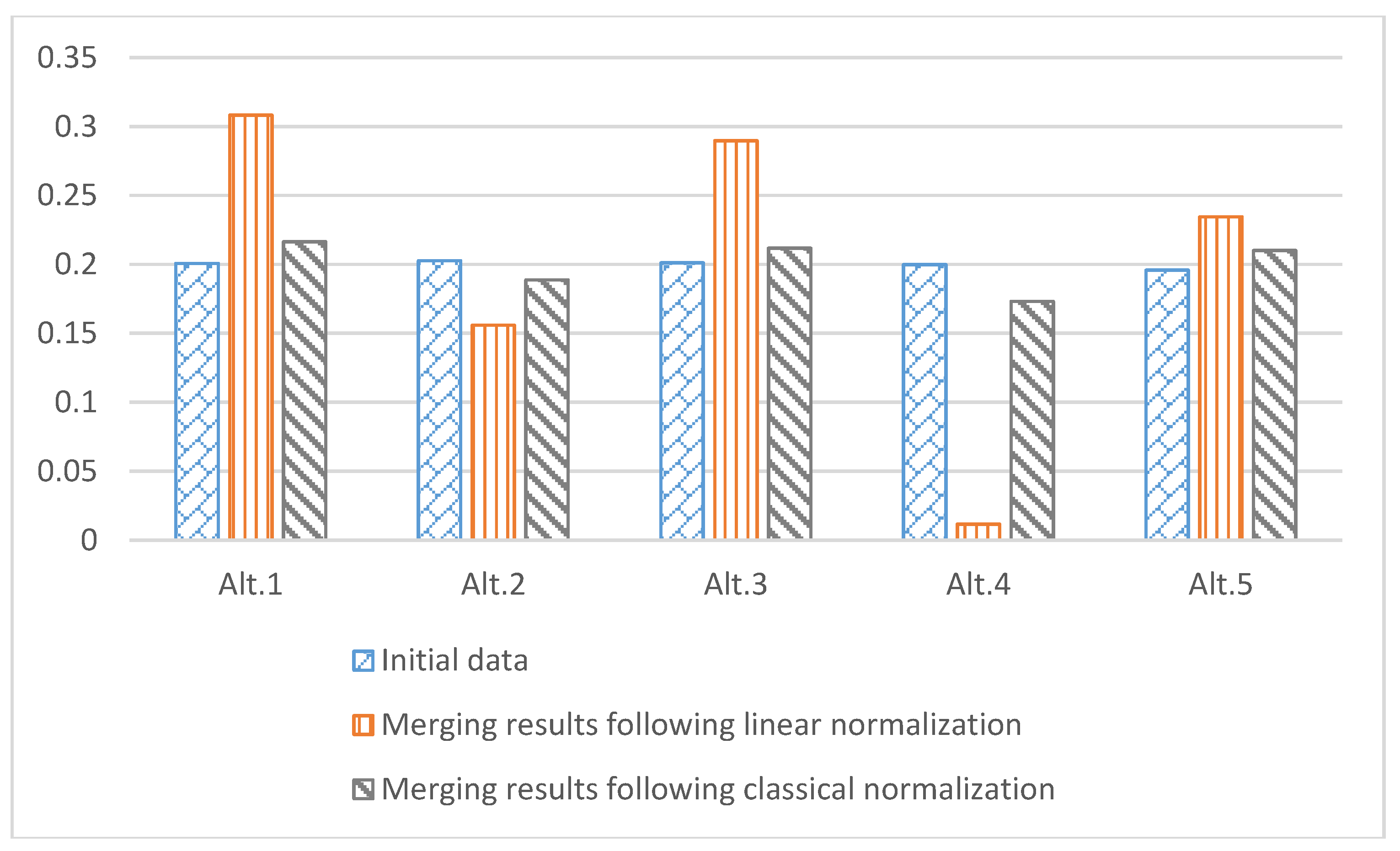
The numerical results of the initial data (Table 1) and the merged results following classical (Figure 6) and linear (Figure 5) normalization are shown in Figure 7.
Before comparing the obtained information, the results were normalized so that the sum of all estimates of alternatives should be equal to one. The chart shows that the means of the estimates of the initial data differ slightly from each other. The merged results demonstrate that linear normalization leads to significant variations in the outcomes, which is clearly expressed in the evaluation of the fourth alternative. Differences in the results obtained following classical normalization are not significantly expressed in the chart.
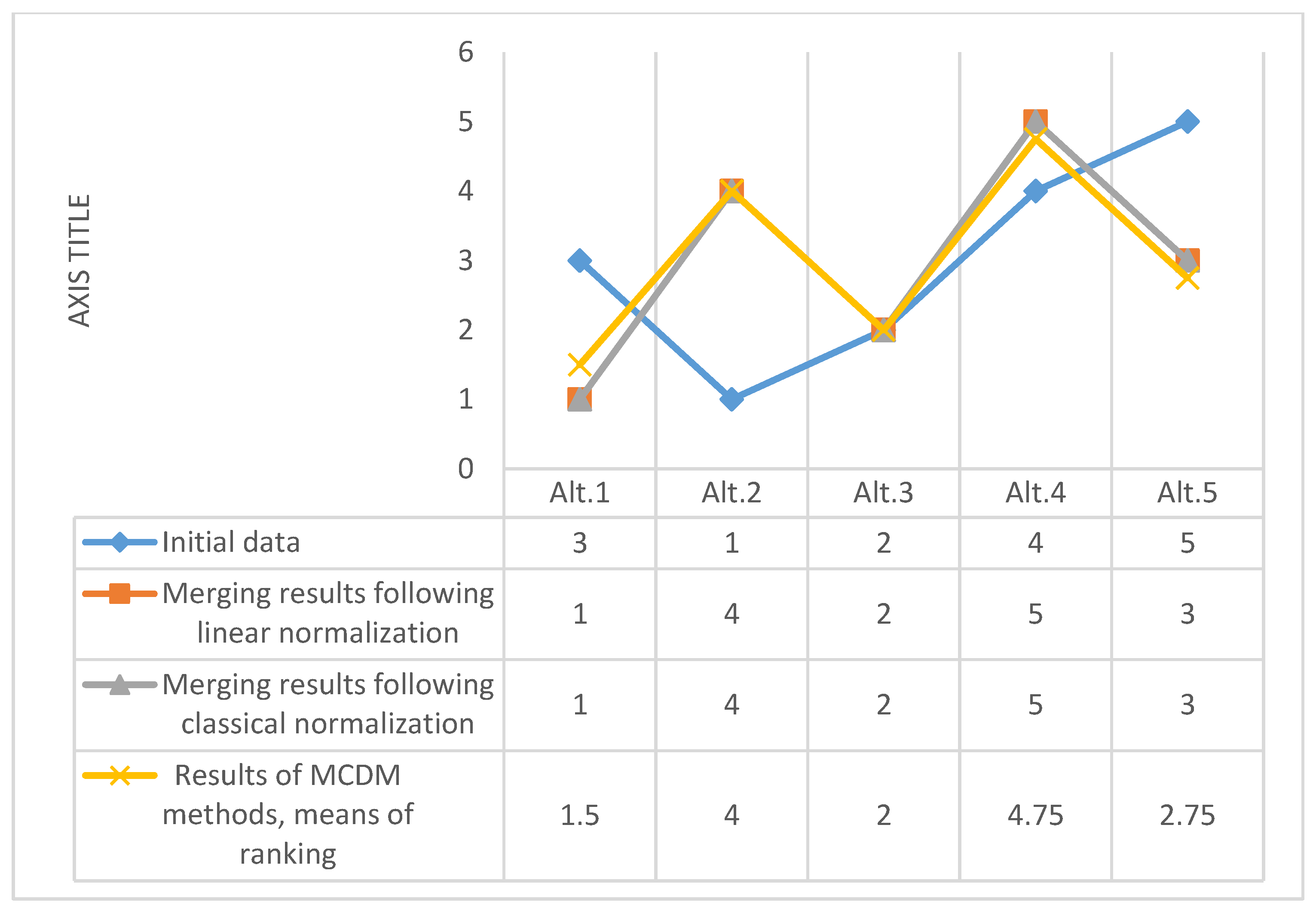
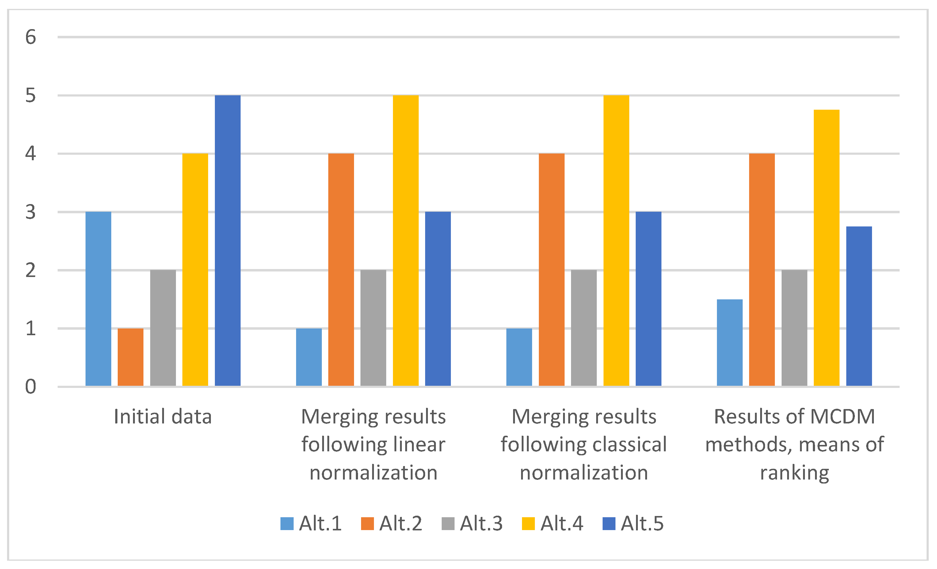
The results expressed in ranks are shown in Figure 8 and Figure 9. These charts indicate the mean ranks of the initial data, the ranks of the results of the merged MADM methods (following linear and classical normalization) and the means of the ranks of the results obtained by employing MADM methods. The best alternative is ranked 1, whereas the worst-rated alternative takes 5.
The results of the initial data differ from those achieved by evaluating the outcomes of the first and second alternatives. The merged results coincided following linear and classical normalization. The mean values of the results of MADM methods mainly coincided with the merged results of MADM methods. Since the values of the weights of MADM methods Ω are similar to each other (Figure 4), they did not have a significant effect on the final result. The average results of MADM ranks of the first and third alternatives may lead to different interpretations due to their estimates being equal to 1.5 and 2. The combined results have unequivocally identified the best alternative as Alt. 1.
Table 3 shows that the sum of the estimates for each alternative is equal to 1, which facilitates comparing them. A comparison of the ranked results provided in Figure 5 and Figure 6 demonstrates that the employed methods of the linear and classical normalization of MADM results have determined all alternatives equally. For comparing the mean values of the initial estimates with the findings obtained using MADM methods, the ranking results have changed due to the effect of criterion weights.
5. Discussion and Conclusions
The paper has considered MADM methods as an integral part of the mathematical optimization theory. To illustrate the idea, some of the most applicable methods, SAW, TOPSIS, MOORA, PROMETHEE and COPRAS, have been preferred, and their evaluation criteria have been presented as objective functions, although this paper’s methodology is not limited to the use of only these methods. Other MADM methods such as VIKOR, ELECTRE, Evaluation Based on Distance from Average Solution (EDAS), etc. can be similarly introduced as objective functions. The forthcoming papers of the author will focus on exploring more extensively the limitations to constraints on the variables of the above-listed and new MADM methods and will concentrate on the properties of the objective functions and their limitations.
The MADM methods introduced in this paper are employed for selecting the best alternative evaluated according to the established criteria. The purpose of classical optimization is analogous to MADM methods presented in the paper, which means finding an optimal solution from several or many possible options. The use of MADM makes sense in comparing alternatives that do not contain any dominant alternatives when considering all evaluation criteria. The data used in the presented MADM methods are not changed by searching for the optimal solution from all available ones. The decision matrix and the vector of criterion weights are static data, and the number of optional alternatives is finite.
Merging the results of the MADM methods in accordance with their importance showed their possibilities in evaluation. There is a large number of MADM methods, and therefore the literature does not provide unambiguous recommendations for the most appropriate one. Therefore, multiple MADM methods are frequently applied in practice. A methodology for merging the results of MADM methods was presented in this paper, based on summing up the normalized MADM results into a single value and considering the methods’ stability.
The findings have demonstrated that weights have a significant influence on the result. In order to analyze the influence of the weights of criteria and methods on the obtained result, a problem example was presented in the practical part of the paper, and the averages of evaluating alternatives had little difference between them. Criterion weights have been found to significantly alter the primary outcomes. The established stability of the applied methods did not differ significantly: ΩSAW = 0.2608, ΩTOPSIS = 0.2625, ΩMOORA = 0.249, ΩPROMETHEE = 0.2277. Nevertheless, the influence of the weights of the methods on the result is noticeable. The ranked result obtained employing the TOPSIS method coincided with the ranked composite result, since the TOPSIS method had a greater influence of weight than the rest of the techniques had. The average results of MADM ranks of the first and third alternatives may lead to different interpretations due to their estimates being equal to 1.5 and 2. The combined results have unequivocally identified the best alternative.
Wietendorf’s linear normalization is appropriate for rearranging the results of different scales as well as for the negative values of the PROMETHEE method. However, linear normalization has a disadvantage. Applying Wietendorf’s linear normalization, the estimate of the worst alternative is converted into zero, and thus the weight of the influence of the method for determining the worst alternative has no effect on the combined result. The result data managed by applying classical normalization are convenient to be compared because the sum of all results is equal to one. In the case of classical normalization, the negative results of the methods require additional data transformation. The author of this paper proposes a method of transforming negative numbers. Hence, the normalization method had no influence on the final combined result in this task.
The article provides a method for verifying the stability of the MADM method, which ensures the validity of the evaluated result. The technique for validating the stability of the MADM method has a wide range of practical usability in different decision-making problems where evaluation is performed by employing several MADM methods. The proposed method considers the uncertainty of data on expert evaluation and therefore decreases the level of the subjectivity of the conducted evaluation. Further papers will focus more intensely on analyzing the sensitivity of fuzzy AHP methods by fluctuating the data and on investigating several algorithms of FAHP methods.
Funding
This research received no external funding.
Conflicts of Interest
The author declares no conflict of interest.
References
- Mardani, A.; Zavadskas, E.K.; Khalifah, Z.; Zakuan, N.; Jusoh, A.; Nor, K.; Khoshnoudi, M. A review of multi-criteria decision-making applications to solve energy management problems: Two decades from 1995 to 2015. Renew. Sustain. Energy Rev. 2017, 71, 216–256. [Google Scholar] [CrossRef]
- Mardani, A.; Jusoh, A.; Nor, K.; Khalifah, Z.; Zakwan, N.; Valipour, A. Multiple criteria decision-making techniques and their applications—A review of the literature from 2000 to 2014. Econ. Res. 2015, 28, 516–571. [Google Scholar] [CrossRef]
- Brans, J.P.; Mareschal, B. PROMETHEE V: MCDM problems with segmentation constraints. INFOR Inf. Syst. Oper. Res. 1992, 30, 85–96. [Google Scholar] [CrossRef]
- Liou, J.J.H.; Tzeng, G.-H. Comments on “Multiple criteria decision making (MCDM) methods in economics: An overview”. Technol. Econ. Dev. Econ. 2012, 18, 672–695. [Google Scholar] [CrossRef]
- Opricovic, S.; Tzeng, G.H. Compromise solution by MCDM methods: A comparative analysis of VIKOR and TOPSIS. Eur. J. Oper. Res. 2004, 156, 445–455. [Google Scholar] [CrossRef]
- Ramani, T.L.; Quadrifoglio, L.; Zietsman, J. Accounting for nonlinearity in the MCDM approach for a transportation planning application. IEEE Trans. Eng. Manag. 2010, 57, 702–710. [Google Scholar] [CrossRef]
- Hwang, C.L.; Yoon, K. Multiple Attribute Decision Making: Methods and Applications a State-of-the-Art Survey; Springer: Berlin/Heidelberg, Germany, 1981. [Google Scholar] [CrossRef]
- Tzeng, G.H.; Huang, J.J. Multiple Attribute Decision Making: Methods and Applications; CRC Press: Boca Raton, FL, USA, 2011. [Google Scholar]
- Chang, Y.H.; Yeh, C.H. Evaluating airline competitiveness using multiattribute decision making. Omega 2001, 29, 405–415. [Google Scholar] [CrossRef]
- Belton, V.; Stewart, T.J. Multiple Criteria Decision Analysis: An Integrated Approach; Kluwer: Alphen aan den Rijn, The Nederlands, 2002. [Google Scholar] [CrossRef]
- Malczewski, J.; Rinner, C. Multiattribute decision analysis methods. In Multicriteria Decision Analysis in Geographic Information Science; Springer: Berlin/Heidelberg, Germany, 2015; pp. 81–121. [Google Scholar] [CrossRef]
- Yeh, C.H.; Deng, H.; Chang, Y.H. Fuzzy multicriteria analysis for performance evaluation of bus companies. Eur. J. Oper. Res. 2000, 126, 459–473. [Google Scholar] [CrossRef]
- Mareschal, B.; Brans, J.P.; Vincke, P. PROMETHEE: A new family of outranking methods in multicriteria analysis. In Proceedings of the 10th Triennial Conference on Operational Research, Washington, DC, USA, 6–10 August 1984. [Google Scholar]
- Zavadskas, E.K.; Podvezko, V. Integrated determination of objective criteria weights in MCDM. Int. J. Inf. Technol. Decis. Mak. 2016, 15, 267–283. [Google Scholar] [CrossRef]
- Podvezko, V. Application of AHP technique. J. Bus. Econ. Manag. 2009, 10, 181–189. [Google Scholar] [CrossRef]
- Taha, H.A. Operations Research: An Introduction, 6th ed.; Prentice Hall: Upper Saddle River, NJ, USA, 1997. [Google Scholar]
- Vinogradova, I.; Kliukas, R. Methodology for evaluating the quality of distance learning courses in consecutive stages. Proc. Soc. Behav. Sci. 2015, 191, 1583–1589. [Google Scholar] [CrossRef]
- Williams, H. Fourier’s method of linear programming and its dual. Am. Math. Mon. 1986, 93, 681–695. [Google Scholar] [CrossRef]
- Jorrand, P.; Sgurev, V. Artificial Intelligence IV: Methodology, Systems, Applications; Elsevier: Amsterdam, The Nederlands, 1990. [Google Scholar] [CrossRef]
- Šipoš, M.; Klaić, Z.; Fekete, K.; Stojkov, M. Review of non-traditional optimization methods for allocation of distributed generation and energy storage in distribution system. Teh. Vjesn. 2018, 25, 294–301. [Google Scholar] [CrossRef]
- Dantzig, G. Maximization of a linear function of variables subject to linear inequalities. In Activity Analysis of Production and Allocation; Koopmans, T.C., Ed.; Wiley: Hoboken, NJ, USA, 1951; pp. 339–347. [Google Scholar]
- Robbins, H.; Monro, S. A stochastic approximation method. Ann. Math. Statist. 1951, 22, 400–407. [Google Scholar] [CrossRef]
- Dreyfus, S.E. Richard Bellman on the birth of dynamic programming. Oper. Res. 2002, 50, 48–51. [Google Scholar] [CrossRef]
- Tan, K.C.; Khor, E.F.; Lee, T.H. Multiobjective Evolutionary Algorithms and Applications; Springer: London, UK, 2005. [Google Scholar] [CrossRef]
- Gunantara, N. A review of multi-objective optimization: Methods and its applications. Elect. Electron. Eng. 2018, 5, 1502242. [Google Scholar] [CrossRef]
- Keeney, R.L.; Raiffa, H. Decision Making with Multiple Objectives Preferences and Value Tradeoffs; Wiley: New York, NY, USA, 1976. [Google Scholar]
- Fishburn, P.C. Methods of estimating additive utilities. Manag. Sci. 1967, 13, 435–453. [Google Scholar] [CrossRef]
- Charnes, A.W.; Cooper, W.W.; Rhodes, E. Measuring the efficiency of decision making units. Eur. J. Oper. Res. 1979, 2, 429–444. [Google Scholar] [CrossRef]
- Zavadskas, E.K.; Turskis, Z.; Kildiene, S. State of art surveys of overviews on MCDM/MADM methods. Technol. Econ. Dev. Econ. 2014, 20, 165–179. [Google Scholar] [CrossRef]
- Bernardo, J.J.; Blin, J.M. A programming model of consumer choice among multi-attributed brands. J. Consum. Res. 1977, 4, 111–118. [Google Scholar] [CrossRef]
- MacCrimmon, K.R. Decision Making among Multiple-Attribute Alternatives: A Survey and Consolidated Approach; RAND Memorandum, RM-4823-ARPA; The RAND Corporation: Santa Monica, CA, USA, 1968. [Google Scholar]
- Podvezko, V. The comparative analysis of MCDA methods SAW and COPRAS. Econ. Eng. Decis. 2011, 22, 134–146. [Google Scholar] [CrossRef]
- Peng, H.; Wang, J.A. Multicriteria group decision-making method based on the normal cloud model with Zadeh’s Z-numbers. IEEE Trans. Fuzzy Syst. 2018, 26, 3246–3260. [Google Scholar] [CrossRef]
- Roy, B. The outranking approach and the foundations of ELECTRE methods. Theory Decis. 1991, 31, 49–73. [Google Scholar] [CrossRef]
- Brans, J.P.; Vincke, P.; Mareschal, B. How to select and how to rank projects: The method. Eur. J. Oper. Res. 1986, 24, 228–238. [Google Scholar] [CrossRef]
- Opricovic, S. Multicriteria Optimization of Civil Engineering Systems; University of Belgrade, Faculty of Civil Engineering: Belgrade, Srbija, 1998. [Google Scholar]
- Zavadskas, E.K.; Turskis, Z.; Antucheviciene, J.; Zakarevicius, A. Optimization of weighted aggregated sum product assessment. Electron. Elect. Eng. 2012, 6, 3–6. [Google Scholar] [CrossRef]
- Kildienė, S.; Kaklauskas, A.; Zavadskas, E. COPRAS based comparative analysis of the European country management capabilities within the construction sector in the time of crisis. J. Bus. Econ. Manag. 2011, 12, 417–434. [Google Scholar] [CrossRef]
- Brauers, W.K.M.; Zavadskas, E.K. The MOORA method and its application to privatization in a transition economy. Control. Cybern. 2006, 35, 445–469. [Google Scholar]
- Turskis, Z.; Keršulienė, V.; Vinogradova, I. A new fuzzy hybrid multi-criteria decision-making approach to solve personnel assessment problems. Case study: Director selection for estates and economy office. Econ. Comput. Econ. Cybern. Stud. Res. 2017, 51, 211–229. [Google Scholar]
- Turskis, Z.; Zavadskas, E.K. A novel method for multiple criteria analysis: Grey additive ratio assessment (ARAS-G) method. Informatica 2010, 21, 597–610. [Google Scholar]
- Turskis, Z.; Zavadskas, E.K. A new fuzzy additive ratio assessment method (ARAS-F). Case study: The analysis of fuzzy multiple criteria in order to select the logistic centers location. Transport 2010, 25, 423–432. [Google Scholar] [CrossRef]
- Krylovas, A.; Zavadskas, E.K.; Kosareva, N.; Dadelo, S. New KEMIRA method for determining criteria priority and weights in solving MCDM problem. Int. J. Inf. Technol. Decis. Mak. 2014, 13, 1119–1133. [Google Scholar] [CrossRef]
- Zavadskas, E.K.; Turskis, Z. A new additive ratio assessment (ARAS) method in multicriteria decision-making. Technol. Econ. Dev. Econ. 2010, 16, 159–172. [Google Scholar] [CrossRef]
- Del Vasto-Terrientes, L.; Valls, A.; Slowinski, R.; Zielniewicz, P. ELECTRE-III-H: An outranking-based decision aiding method for hierarchically structured criteria. Expert Syst. Appl. 2015, 42, 4910–4926. [Google Scholar] [CrossRef]
- Corrente, S.; Greco, S.; Slowinski, R. Multiple criteria hierarchy process with ELECTRE and PROMETHEE. Omega 2013, 41, 820–846. [Google Scholar] [CrossRef]
- Ziemba, P. Towards strong sustainability management—A generalized PROSA method. Sustainability 2019, 11, 1555. [Google Scholar] [CrossRef]
- Keršulienė, V.; Zavadskas, E.K.; Turskis, Z. Selection of rational dispute resolution method by applying new stepwise weight assessment ratio analysis (SWARA). J. Bus. Econ. Manag. 2010, 11, 243–258. [Google Scholar] [CrossRef]
- Trinkūnienė, E.; Podvezko, V.; Zavadskas, E.K.; Jokšienė, I.; Vinogradova, I.; Trinkūnas, V. Evaluation of quality assurance in contractor contracts by multi-attribute decision-making methods. Econ. Res. Ekon. Istraž. 2017, 30, 1152–1180. [Google Scholar] [CrossRef] [Green Version]
- Saaty, T.L. The Analytic Hierarchy Process; McGraw-Hill: New York, NY, USA, 1980. [Google Scholar]
- Saaty, T.L. The analytic hierarchy and analytic network processes for the measurement of intangible criteria and for decision-making. In Multiple Criteria Decision Analysis: State of the Art Surveys; Greco, S., Ehrgott, M., Figueira, J., Eds.; Springer: Berlin, Germany, 2005; pp. 345–408. [Google Scholar] [CrossRef]
- Kurilov, J.; Vinogradova, I. Improved fuzzy AHP methodology for evaluating quality of distance learning courses. Int. J. Eng. Educ. 2016, 32, 1618–1624. [Google Scholar] [CrossRef]
- Kurilovas, E.; Vinogradova, I.; Kubilinskiene, S. New MCEQLS fuzzy AHP methodology for evaluating learning repositories: A tool for technological development of economy. Technol. Econ. Dev. Econ. 2016, 22, 142–155. [Google Scholar] [CrossRef]
- Hashemkhani, Z.; Saparauskas, J. New application of SWARA method in prioritizing sustainability assessment indicators of energy system. Inz. Ekon. Eng. Econ. 2013, 24, 408–414. [Google Scholar] [CrossRef]
- Čereška, A.; Zavadskas, E.K.; Bucinskas, V.; Podvezko, V.; Sutinys, E. Analysis of steel wire rope diagnostic data applying multi-criteria methods. Appl. Sci. 2018, 8, 260. [Google Scholar] [CrossRef]
- Vinogradova, I.; Podvezko, V.; Zavadskas, E.K. The recalculation of the weights of criteria in MCDM methods using the Bayes approach. Symmetry 2018, 10, 205. [Google Scholar] [CrossRef]
- Sabaei, D.; Erkoyuncu, J.; Roy, R. A review of multi-criteria decision making methods for enhanced maintenance delivery. Proc. CIRP 2015, 37, 30–35. [Google Scholar] [CrossRef]
- Stewart, T.J. A critical survey on the status of multiple criteria decision making theory and practice. Omega 1992, 20, 569–586. [Google Scholar] [CrossRef]
- Kim, J.; Kim, J. Optimal portfolio for LNG importation in Korea using a two-step portfolio model and a fuzzy analytic hierarchy process. Energies 2018, 11, 3049. [Google Scholar] [CrossRef]
- Adeel, A.; Akram, M.; Ahmed, I.; Nazar, K. Novel m-polar fuzzy linguistic ELECTRE-I method for group decision-making. Symmetry 2019, 11, 471. [Google Scholar] [CrossRef]
- Bae, H.J.; Kang, J.E.; Lim, Y.R. Assessing the health vulnerability caused by climate and air pollution in Korea using the fuzzy TOPSIS. Sustainability 2019, 11, 2894. [Google Scholar] [CrossRef]
- Ziemba, P.; Becker, J. Analysis of the digital divide using fuzzy forecasting. Symmetry 2019, 11, 166. [Google Scholar] [CrossRef]
- Evans, J.R. Sensitivity analysis in decision theory. Decis. Sci. 1984, 15, 239–247. [Google Scholar] [CrossRef]
- Barron, H.; Schmidt, C.P. Sensitivity analysis of additive multiattribute value models. Oper. Res. 1988, 36, 122–127. [Google Scholar] [CrossRef]
- Insua, D.R. Sensitivity Analysis in Multi-Objective Decision Making; Springer: Berlin/Heidelberg, Germany, 1990. [Google Scholar] [CrossRef]
- Janssen, R. Multiobjective Decision Support for Environmental Management; Kluwer: Alphen aan den Rijn, The Nederlands, 1992. [Google Scholar] [CrossRef]
- Butler, J.; Jia, J.; Dyer, J. Simulation techniques for the sensitivity analysis of multi-criteria decision models. Eur. J. Oper. Res. 1997, 103, 531–546. [Google Scholar] [CrossRef]
- Wolters, W.T.M.; Mareschal, B. Novel types of sensitivity analysis for additive MCDM methods. Eur. J. Oper. Res. 1995, 81, 281–290. [Google Scholar] [CrossRef] [Green Version]
- Masuda, T. Hierarchical sensitivity analysis of the priorities used in the analytic hierarchy process. Int. J. Syst. Sci. 1990, 21, 415–427. [Google Scholar] [CrossRef]
- Triantaphyllou, E.; Sánchez, A. A sensitivity analysis approach for some deterministic multi-criteria decision-making methods. Decis. Sci. 1997, 28, 151–194. [Google Scholar] [CrossRef]
- Podvezko, V. Multicriteria evaluation under uncertainty. Bus. Theory Pract. 2006, 7, 81–88. (In Lithuanian) [Google Scholar] [CrossRef]
- Zavadskas, E.K.; Turskis, Z.; Dejus, T.; Viteikiene, M. Sensitivity analysis of a simple additive weight method. Int. J. Manag. Decis. Mak. 2007, 8, 555–574. [Google Scholar] [CrossRef]
- Memariani, A.; Amini, A.; Alinezhad, A. Sensitivity analysis of simple additive weighting method (SAW): The results of change in the weight of one attribute on the final ranking of alternatives. J. Ind. Eng. 2009, 4, 13–18. [Google Scholar]
- Alinezhad, A.; Sarrafha, K.; Amini, A. Sensitivity analysis of SAW technique: The impact of changing the decision making matrix elements on the final ranking of alternatives. Iran. J. Oper. Res. 2014, 5, 82–94. [Google Scholar]
- Yu, V.F.; Hu, K.J. An integrated fuzzy multi-criteria approach for the performance evaluation of multiple manufacturing plants. Comput. Ind. Eng. 2010, 58, 269–277. [Google Scholar] [CrossRef]
- Alinezhada, A.; Aminib, A. Sensitivity analysis of TOPSIS technique: The results of change in the weight of one attribute on the final ranking of alternatives. J. Optim. Ind. Eng. 2011, 7, 23–28. [Google Scholar]
- Misra, S.K.; Ray, A. Comparative study on different multi-criteria decision making tools in software project selection scenario. Int. J. Adv. Res. Comput. Sci. 2012, 3, 172–178. [Google Scholar] [CrossRef]
- Moghassem, A.R. Comparison among two analytical methods of multi-criteria decision making for appropriate spinning condition selection. World Appl. Sci. J. 2013, 21, 784–794. [Google Scholar]
- Hsu, L.C.; Ou, S.L.; Ou, Y.C. A comprehensive performance evaluation and ranking methodology under a sustainable development perspective. J. Bus. Econ. Manag. 2015, 16, 74–92. [Google Scholar] [CrossRef]
- Podvezko, V.; Podviezko, A. Dependence of multi-criteria evaluation result on choice of preference functions and their parameters. Technol. Econ. Dev. Econ. 2010, 16, 143–158. [Google Scholar] [CrossRef]
- Zavadskas, E.K.; Kaklauskas, A.; Peldschus, F.; Turskis, Z. Multi-attribute assessment of road design solutions by using the COPRAS method. Balt. J. Road Bridge Eng. 2007, 2, 195–203. [Google Scholar]
- Weitendorf, D. Beitrag Zur Optimierung Der Räumlichen Struktur Eines Gebäudes. Ph.D. Thesis, Hochschule für Architektur und Bauwesen, Weimar, Germany, 1976. [Google Scholar]
- Zavadskas, E.K.; Turskis, Z. A new logarithmic normalization method in games theory. Informatica 2008, 19, 303–314. [Google Scholar]
- Vinogradova, I. Integration of several MCDM results according to the importance of methods. Liet. Matem. Rink. LMD Darb. B 2016, 57, 77–82. (In Lithuanian) [Google Scholar]
Figure 1.
Function charts of criterion priorities: (a) function chart of the priorities of the usual criterion; (b) function chart of the priorities of the U-shape criterion; (c) function chart of the priorities of the V-shape criterion; (d) function chart of the priorities of the level criterion; (e) function chart of the priorities of the V-shape with indifference criterion; (f) function chart of the priorities of the Gaussian criterion.

Figure 2.
The algorithm for evaluating the stability of the Multi-Attribute Decision-Making (MADM) method.
Figure 2.
The algorithm for evaluating the stability of the Multi-Attribute Decision-Making (MADM) method.

Figure 3.
The results obtained using MADM methods. SAW: Simple Additive Weighting; TOPSIS: Technique for Order of Preference by Similarity to Ideal Solution; MOORA: Multi-Objective Optimization by Ratio Analysis; PROMETHEE: Preference Ranking Organization Method for Enrichment Evaluation.
Figure 3.
The results obtained using MADM methods. SAW: Simple Additive Weighting; TOPSIS: Technique for Order of Preference by Similarity to Ideal Solution; MOORA: Multi-Objective Optimization by Ratio Analysis; PROMETHEE: Preference Ranking Organization Method for Enrichment Evaluation.

Figure 4.
A comparison of stability determined by applying MADM methods.

Figure 5.
Merging the results of MADM methods following linear normalization.

Figure 6.
Merging the results of MADM methods following classical normalization.

Figure 7.
The results of evaluating alternatives, means of numerical values.

Figure 8.
The results of evaluating alternatives, means of the ranked values.

Figure 9.
A comparison of the results of evaluating alternatives.


Table 1.
Data on assessing course units.
| w | Number of the Criterion | Alt. 1 | Alt. 2 | Alt. 3 | Alt. 4 | Alt. 5 | |
|---|---|---|---|---|---|---|---|
| 0.27 | max | 1-clearly produced lecture material | 9.00 | 9.00 | 10.00 | 8.75 | 9.20 |
| 0.11 | max | 2-arrangement of studies | 9.00 | 9.50 | 8.00 | 10.00 | 7.75 |
| 0.33 | max | 3-competent teaching staff | 9.75 | 9.40 | 9.25 | 9.75 | 10.00 |
| 0.17 | max | 4-relevance and practical benefits of the material | 9.25 | 8.75 | 9.00 | 7.00 | 8.75 |
| 0.05 | max | 5-variety of techniques for presenting material | 9.25 | 10.00 | 9.50 | 10.00 | 9.50 |
| 0.07 | max | 6-knowledge testing assignments | 9.25 | 9.40 | 9.60 | 9.75 | 9.00 |
| Mean of estimates | 9.25 | 9.34 | 9.27 | 9.21 | 9.03 | ||
| Ranking | 3 | 1 | 2 | 4 | 5 | ||
Table 2.
Normalized MADM result in the range of [0, 1].
| Methods | Alt. 1 | Alt. 2 | Alt. 3 | Alt. 4 | Alt. 5 |
|---|---|---|---|---|---|
| SAW | 1 | 0.66563 | 0.9609 | 0 | 0.6375 |
| TOPSIS | 1 | 0.68297 | 0.9895 | 0 | 0.7424 |
| MOORA | 0.98925 | 0.57617 | 1 | 0 | 0.6322 |
| PROMETHEE | 0.92816 | 0 | 0.7145 | 0.1626 | 1 |
Table 3.
Transformed MADM results applying classical normalization.
| Methods | Alt. 1 | Alt. 2 | Alt. 3 | Alt. 4 | Alt. 5 |
|---|---|---|---|---|---|
| SAW | 0.2022 | 0.2001 | 0.2020 | 0.1958 | 0.1999 |
| TOPSIS | 0.2287 | 0.2000 | 0.2278 | 0.1381 | 0.2054 |
| MOORA | 0.2036 | 0.1993 | 0.2037 | 0.1934 | 0.1999 |
| PROMETHEE | 0.2321 | 0.1509 | 0.2134 | 0.1652 | 0.2384 |
© 2019 by the author. Licensee MDPI, Basel, Switzerland. This article is an open access article distributed under the terms and conditions of the Creative Commons Attribution (CC BY) license (http://creativecommons.org/licenses/by/4.0/).
Share and Cite
MDPI and ACS Style
Vinogradova, I. Multi-Attribute Decision-Making Methods as a Part of Mathematical Optimization. Mathematics 2019, 7, 915. https://0-doi-org.brum.beds.ac.uk/10.3390/math7100915
AMA Style
Vinogradova I. Multi-Attribute Decision-Making Methods as a Part of Mathematical Optimization. Mathematics. 2019; 7(10):915. https://0-doi-org.brum.beds.ac.uk/10.3390/math7100915
Chicago/Turabian StyleVinogradova, Irina. 2019. "Multi-Attribute Decision-Making Methods as a Part of Mathematical Optimization" Mathematics 7, no. 10: 915. https://0-doi-org.brum.beds.ac.uk/10.3390/math7100915
Note that from the first issue of 2016, this journal uses article numbers instead of page numbers. See further details here.