Lattice-Boltzmann Simulations of the Convection-Diffusion Equation with Different Reactive Boundary Conditions

Abstract

We have tested the accuracy and stability of lattice-Boltzmann (LB) simulations of the convection-diffusion equation in a two-dimensional channel flow with reactive-flux boundary conditions. We compared several different implementations of a zero-concentration boundary condition using the Two-Relaxation-Time (TRT) LB model. We found that simulations using an interpolation of the equilibrium distribution were more stable than those based on Multi-Reflection (MR) boundary conditions. We have extended the interpolation method to include mixed boundary conditions, and tested the accuracy and stability of the simulations over a range of Damköhler and Péclet numbers.

1. Introduction

The lattice Boltzmann method (LBM) has been used primarily to solve fluid dynamics problems [1,2,3,4], but it can also be used to approximate solutions of the convection-diffusion equation for a scalar field C [5],

$${\partial }_{t}C+\mathit{u}·\mathbf{\nabla }C=D{\nabla }^{2}C.$$

(1)

In this paper we envisage C as describing a reactant concentration that is sufficiently dilute that it does not affect the flow, but advects and diffuses as a passive scalar in a predetermined velocity field u. There is a growing interest in geophysical applications involving reactant transport, where the surrounding solid matrix dissolves or precipitates [6,7,8,9,10,11]. Typically the time scale for a significant displacement of the solid-fluid interface is much longer than the characteristic time scales for momentum or reactant transport, and in such circumstances it is the stationary limit of (1) that is of most interest.

Lattice-Boltzmann models typically have more degrees of freedom than the macroscopic equations they are trying to simulate. It is therefore problematic how to establish boundary conditions on the population densities so as to best satisfy the macroscopic conditions without polluting the solution with perturbations that, although small on the macroscopic scale, are still significant in a simulation with limited resolution. There is a trade off between first-order boundary conditions, which maintain the exact conservation laws [12,13,14,15] and higher-order methods [16,17,18,19]. In [19], a second-order accurate treatment of the boundary condition in the LB method is developed for a curved boundary. In a seminal paper [17], Ginzburg and d’Humieres proposed a general interpolation scheme that incorporated several earlier schemes as special cases; the most sophisticated Multi-Reflection (MR) schemes are more accurate than alternative methods, at least in simple geometries.

A disadvantage of multi-Reflection boundary conditions is that they require several nodes to implement; up to three in the most accurate cases although two nodes can give accurate results when coupled with a suitable tuning of the kinetic modes of the LB model [17]. However under certain conditions it is not possible to find any neighboring fluid nodes and in such cases the interpolation scheme breaks down [18]; the bounce-back rule is usually invoked for these nodes, but unfortunately this reduces the accuracy of the global solution to something akin to the bounce-back rule [18]. Higher-order local boundary conditions, which make use of information contained in the kinetic modes, have been proposed [18,20], but they have not been used very extensively, perhaps because they are more complicated to implement.

In a Chapman-Enskog analysis, the velocity distribution $f_q(\mathit{r},t)$ is decomposed into an equilibrium part $f_q^{eq}$, which depends on the macroscopic variables, and a non-equilibrium part $f_q^{neq}=f_q-f_q^{eq}$. Since $f_q^{neq}$ depends on gradients of the macroscopic variables, a consistent approximation to the macroscopic fields can be obtained if the non-equilibrium distribution is evaluated at one order lower (in gradients of the macroscopic variables) than the equilibrium distribution. Since the equilibrium distribution can be determined at the solid-fluid boundary, there is an additional node for interpolation, so that only a single fluid node is required as in the case of the bounce-back rule itself. This idea underpins several different improvements to the bounce-back rule [21,22,23]; in this paper we focus on the first implementation [21], which proves to be the most stable.

The convection-diffusion equation is difficult to solve numerically because the Péclet number for reactive transport on a length scale l, $Pe=ul/D$, is typically three orders of magnitude larger than the corresponding Reynolds number $Re=ul/\nu$. Thus the stability of the numerical scheme is of paramount importance for an efficient implementation. Lattice-Boltzmann schemes have the advantage that errors due to numerical dispersion are eliminated, but since the method is explicit it is impossible to ensure stability at high flow rates as the standard upwind finite difference methods do. In this paper we assess the accuracy and stability of the TRT LB model in a simple geometry, to test the accuracy and stability of different implementations of the boundary conditions. We focus on MR schemes for scalar transport [24] and an interpolation of the equilibrium distribution (EQI) along the lines of Refs. [21,25].

This paper is organized as follows. In Section 2, the TRT lattice Boltzmann model for the steady convection-diffusion flow is introduced. The non-equilibrium extrapolation method for the convection is proposed for the Dirichlet or mixed boundary conditions in Section 3 and Section 4. This method combined with finite difference method is easy to implement and can be used for stationary and moving boundary. To demonstrate the numerical accuracy and stability, the steady convection-diffusion flow in long channel is carried on in Section 5. From the simulation results, good agreement with the analytic solution can be seen and this method is of better stability for high $Pe$ number compared to the methods by Ginzburg. Section 6 has a short conclusion of the paper.

2. TRT Model

Lattice Boltzmann models are defined by a set of Q velocities ${\mathit{c}}_q$, ($q=0,1,\dots ,Q-1$), with displacements ${\mathit{b}}_q={\mathit{c}}_{q}h$ that are basis vectors of a crystallographic lattice; here h is the time step of the LB update. The TRT model is a subset of the Multi-Relaxation-Time (MRT) LB models, which maintains the accuracy of MRT LB but with a significantly simpler collision operator. At steady state the TRT equation for the populations $f_q(\mathit{r})$ is [17]

$$f_q({\mathit{r}}_q^{+})=f_q^{*}(\mathit{r})=f_q(\mathit{r})+{\lambda }^{+}{f}_q^{neq,+}(\mathit{r})+{\lambda }^{-}{f}_q^{neq,-}(\mathit{r}),$$

(2)

where $f_q^{*}$ is the post-collision distribution, ${\mathit{r}}_q^{\pm }=\mathit{r}\pm h{\mathit{c}}_q$, $f_q^{neq}=f_q-f_q^{eq}$, and $f_q^{eq}$ is the equilibrium distribution. The symmetric and anti-symmetric populations are given by

$$f_q^{\pm }=\frac{1}{2}\left(f_q\pm f_{\overline{q}}\right),$$

(3)

with ${\mathit{c}}_{\overline{q}}=-{\mathit{c}}_q$. At steady state $f_0^{neq}=0$ [26], and $f_0=f_0^{eq}=t_{0}C$.

The steady-state convection-diffusion equation is most accurately simulated with a linear equilibrium distribution of the form

$$f_q^{eq}=t_{q}C\left(1+\frac{\mathit{u}·{\mathit{c}}_q}{\alpha c^2}\right),$$

(4)

where $C(\mathit{r})$ is the concentration field and $\mathit{u}(\mathit{r})$ is the imposed velocity field; for a grid spacing of b, $c=b/h$. The parameter $\alpha$ typically takes the value $\alpha =1/3$, but it can be reduced to increase the range of stability, subject to the limitations indicated in

Table 1. Coefficents $t_q$ for various LB models. The weights for the different speeds are shown for each model, together with the largest possible value of $\alpha$, $0<\alpha <{\alpha }_{max}$ and the coefficient of the fourth-order isotropic term A.

Model	${\mathit{t}}_0$	${\mathit{t}}_1$	${\mathit{t}}_{\sqrt{2}}$	${\mathit{t}}_{\sqrt{3}}$	${\mathit{\alpha }}_{\mathit{max}}$	A
D1Q3	$1-\alpha$	$\frac{1}{2}\alpha$			1	$\frac{1}{3}\alpha$
D2Q7	$1-2\alpha$	$\frac{1}{3}\alpha$			$\frac{1}{2}$	$\frac{3}{4}\alpha$
D2Q9	$1-\frac{5}{3}\alpha$	$\frac{1}{3}\alpha$	$\frac{1}{12}\alpha$		$\frac{3}{5}$	$\frac{1}{3}\alpha$
D3Q15	$1-\frac{7}{3}\alpha$	$\frac{1}{3}\alpha$		$\frac{1}{24}\alpha$	$\frac{3}{7}$	$\frac{1}{3}\alpha$
D2Q19	$1-2\alpha$	$\frac{1}{6}\alpha$	$\frac{1}{12}\alpha$		$\frac{1}{2}$	$\frac{1}{3}\alpha$

. In general the velocity field is found from an independent simulation, but in this investigation we impose a Poiseuille-flow profile in a channel of width H, $u_x(y)=4u_{0}y(H-y)/H^2$; the Péclet number is based on the average velocity in the channel

$$Pe=\frac{2u_{0}H}{3D}.$$

(5)

LB simulations of time-dependent convection-diffusion include a non-linear term in the equilibrium distribution to eliminate second-order errors in the evolving concentration field. However, this contribution actually introduces a second-order error in the steady-state solution, where the time-scale separation assumed in the Chapman-Enskog expansion is no longer entirely valid [27].

The coefficients $t_q$ (Table 1) must satisfy the following sum rules to obtain the correct macroscopic behavior:

$$\begin{array}{cc}\hfill \sum _q{t}_q& =1,\hfill \\ \hfill \sum _q{t}_q{c}_{q,i}{c}_{q,j}& =\alpha c^2{\delta }_{ij},\hfill \\ \hfill \sum _q{t}_q{c}_{q,i}{c}_{q,j}{c}_{q,k}{c}_{q,l}& =A{c}^4({\delta }_{ij}{\delta }_{kl}+{\delta }_{ik}{\delta }_{jl}+{\delta }_{il}{\delta }_{jk}).\hfill \end{array}$$

(6)

The first two moments of $f_q^{eq}$ are:

$$\sum _q{f}_q=\sum _q{f}_q^{eq}=C,\sum _q{f}_q{\mathit{c}}_q=\sum _q{f}_q^{eq}{\mathit{c}}_q=\mathit{u}C,$$

(7)

while for mass-conserving collisions ${\sum }_q{f}_q^{neq}=0$.

The macroscopic behavior (at steady state) can be found from a Taylor expansion of Equation (2) about r, which leads to a hierarchy of moment equations, which are truncated systematically at order $h^4$:

$$\begin{array}{cc}\hfill h\mathbf{\nabla }·{\mathit{m}}_1+\frac{h^2}{2}\mathbf{\nabla }\mathbf{\nabla }:{\mathit{m}}_2+\frac{h^3}{6}\mathbf{\nabla }\mathbf{\nabla }\mathbf{\nabla }:{\mathit{m}}_3^{eq}+\mathcal{O}(h^4)& ={\lambda }^{+}{\mathit{m}}_0^{neq}=0,\hfill \end{array}$$

(8)

$$\begin{array}{cc}\hfill h\mathbf{\nabla }·{\mathit{m}}_2+\frac{h^2}{2}\mathbf{\nabla }\mathbf{\nabla }:{\mathit{m}}_3^{eq}+\mathcal{O}(h^3)& ={\lambda }^{-}{\mathit{m}}_1^{neq},\hfill \end{array}$$

(9)

$$\begin{array}{cc}\hfill h\mathbf{\nabla }·{\mathit{m}}_3^{eq}+\mathcal{O}(h^2)& ={\lambda }^{+}{\mathit{m}}_2^{neq}.\hfill \end{array}$$

(10)

The moments ${\mathit{m}}_n={\sum }_q{f}_q{\mathit{c}}_q^n$ can be separated into equilibrium $\mathcal{O}(1)$ and non-equilibrium $\mathcal{O}(h)$ contributions. Substituting explicit expressions for the equilibrium moments (4) and solving Equation (9) for ${\mathit{m}}_1^{neq}$ we obtain the convection-diffusion equation with second-order errors:

$$\mathbf{\nabla }·(\mathit{u}C)=D{\nabla }^{2}C-h^2{c}^2\left({\Lambda }^{+}{\Lambda }^{-}-\frac{1}{12}\right){\nabla }^2\mathbf{\nabla }·(\mathit{u}C)+\mathcal{O}(h^3),$$

(11)

where ${\Lambda }^{\pm }=-(1/{\lambda }^{\pm }+1/2)$ and $D=\alpha {\Lambda }^{-}h{c}^2$. The steady-state solution is third-order accurate if $\Lambda ={\Lambda }^{+}{\Lambda }^{-}=1/12$ and second order otherwise.

The location of the solid-fluid boundary depends on ${\Lambda }^{\pm }$, but for bounce-back and related boundary conditions the macroscopic fields are independent of $\Lambda ={\Lambda }^{+}{\Lambda }^{-}$ if the product $\Lambda ={\Lambda }^{+}{\Lambda }^{-}$ is held fixed [17,24]. Although there is no single value of $\Lambda$ that ensures that even planar boundaries are located in exactly the correct place, the choice $\Lambda =1/4$ gives a near optimum boundary condition for arbitrary geometries [17,24]. It is possible to solve for the steady-state concentration field directly [28], but here we use standard time-stepping algorithm to reach the steady solution.

3. Dirichlet Boundary Conditions

We have tested different implementations of a Dirichlet boundary condition for reactive transport in a two-dimensional channel flow. The focus is on the accuracy and stability of the simulation when the grid Péclet number,

$$P{e}_g=\frac{2u_{0}b}{3D},$$

(12)

is larger than 1. The concentration profile at the inlet is Gaussian,

$$C(0,y)=exp\left[-\frac{{(y-H/2)}^2}{2{\sigma }^2}\right],$$

(13)

with $\sigma =0.1H$; this eliminates singularities in the concentration field at the corners of the channel. At the outlet we implement a no-flux condition ${\partial }_{x}C=0$, but the system is always sufficiently large so that the concentration at the outlet was entirely negligible. We have investigated the “anti-bounce-back” (ABB) rule [24], 2nd and 3rd order implementations of the Multi-Reflection boundary condition [24], and an interpolation of the equilibrium distribution [21].

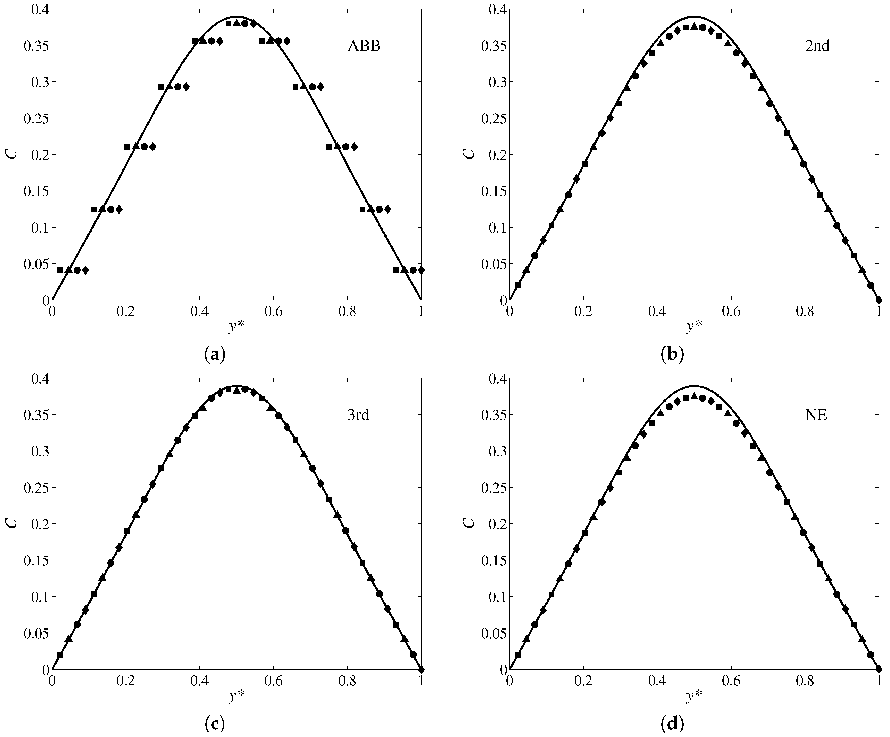
A typical set of results is illustrated in Figure 1 which shows the concentration profile across the channel a short distance from the inlet. The channel width is set to 10 grid points, $H=11b$, and the channel boundaries are placed at different locations with respect to the fluid grid. At sufficiently high Péclet numbers axial diffusion can be neglected and the concentration profile can then be approximated by a series solution that converges very rapidly away from the inlet. However, for $Pe<100$, axial diffusion is not entirely negligible so we have used a high resolution ($H=160b$) simulation for our “exact” results; we verified that this solution approaches the analytic series expansion in the limit of large Péclet number (i.e., $Pe>100$). As expected the ABB rules are only accurate when $q=0.5$, whereas interpolated boundary conditions (2nd, 3rd, NE) are more or less independent of the location of the boundary. There is a small, $\mathcal{O}{(b/H)}^2$, error in both second-order methods (2nd and NE) near the centerline, while the 3rd-order method has a significantly smaller error.

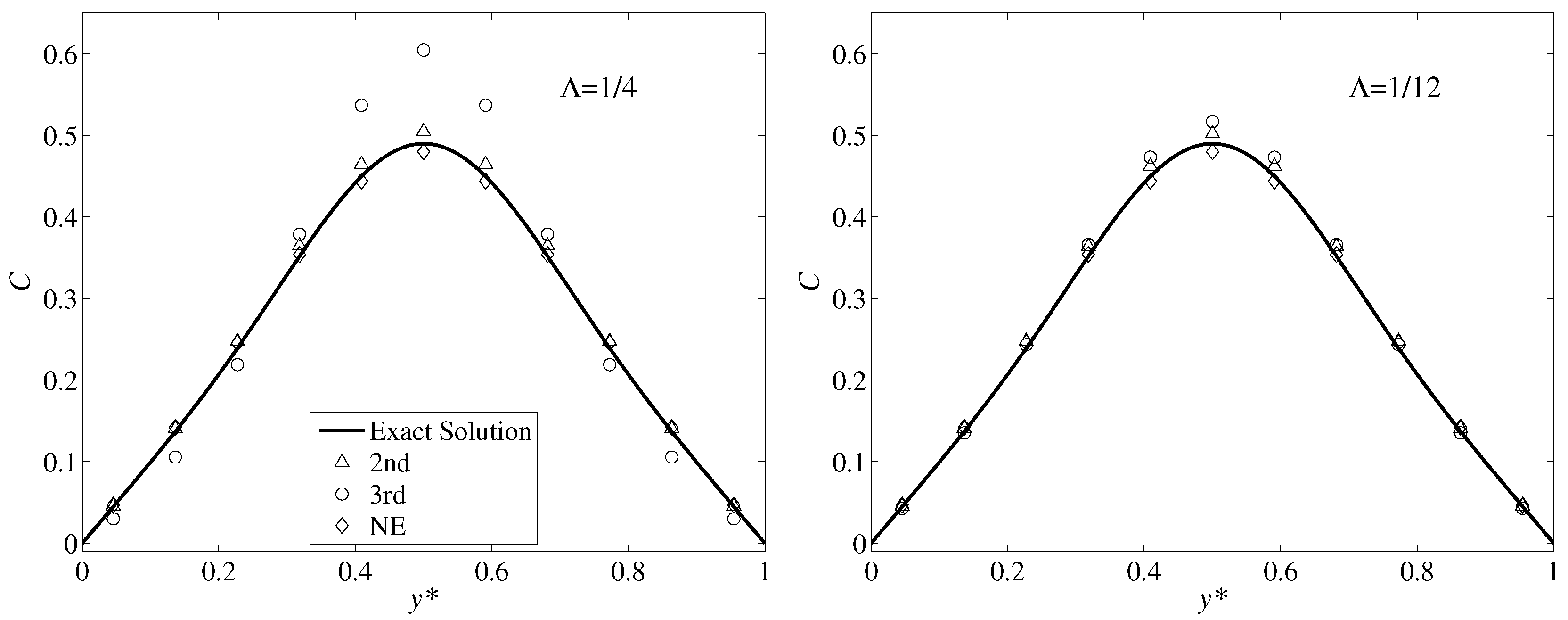
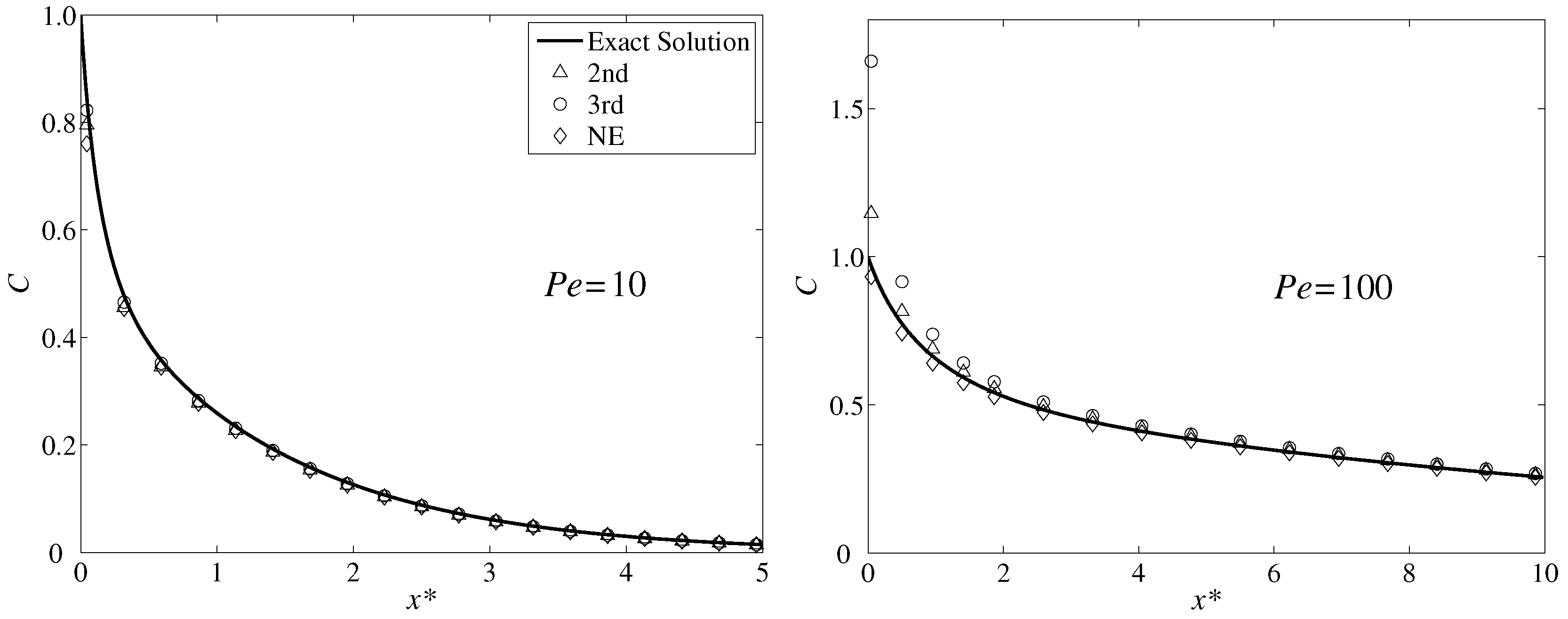
Surprisingly, at larger Péclet numbers ($Pe=100$) there are significant errors in the 3rd-order solution near the centerline, as illustrated in Figure 2; on the other hand the second-order solutions maintain a similar accuracy at the higher Péclet number. The error in the 3rd-order boundary condition is reduced by taking $\Lambda =1/12$, which makes the LB model third-order accurate in the bulk (11) as well as at the boundary. Since the largest error in concentration is in the middle of the channel, in Figure 3 we plot the centerline concentration as a function of the axial coordinate $x^{*}=x/H$. At the lower Péclet number all three methods produce similar results, with the 3rd-order method being the most accurate, but at $Pe=100$ only the non-equilibrium extrapolation (NE) produces an accurate result near the inlet.

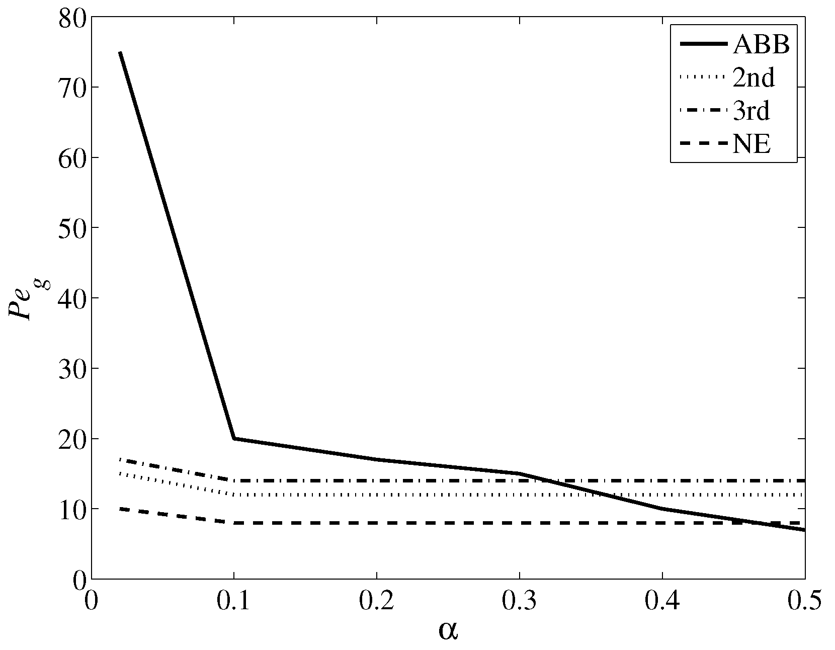
Large errors near the inlet at high-Péclet numbers may be connected to the onset of an instability in the evolving concentration field. Figure 4 shows an approximate stability diagram, delineating regions where stable solutions can be obtained for different values of $\alpha$ (4). The 3rd-order Multi-Reflection boundary condition is the least stable in these simulations, never quite reaching a grid Péclet number $P{e}_g=10$; simulations with $Pe=100$ in a channel of width $11b$ are therefore at the margin of stability. The 2nd-order MR and ABB methods are more stable, with maximum grid Péclet numbers of 18 and 15 respectively; again the stability is insensitive to the choice of $\alpha$. However, the NE method reaches a much higher grid Péclet number $P{e}_g=75$ when $\alpha$ is sufficiently small ($\alpha =0.025$). Thus the NE boundary condition appears to be the most suitable for high-Péclet transport; we will focus on this method in subsequent sections.

4. Mixed Boundary Conditions

The general form for the reactive boundary condition with linear reaction kinetics is

$$D\mathit{n}·\mathbf{\nabla }C=kC,$$

(14)

where n is the surface normal pointing into the fluid and k is the reaction rate constant. A general implementation of these boundary conditions has been derived based on the Multi-Reflection boundary conditions [24], but since these are less stable than the extrapolation method [21] we will not consider them further. Alternative interpolation schemes [22,23] will reduce to the anti-bounce-back rule when $\delta =1/2$; thus they will also be unable to reach grid Péclet numbers in excess of 20.

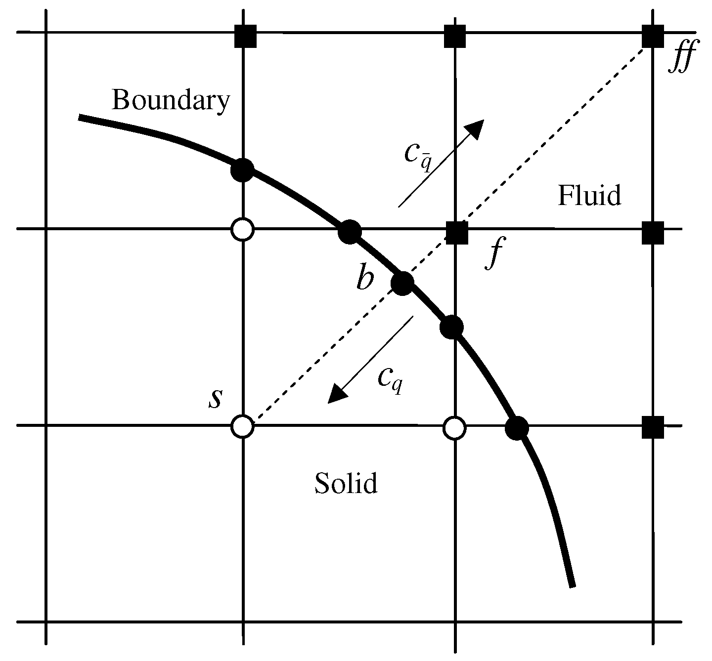
The boundary condition is implemented in two stages; first the concentration at the boundary satisfying (14) is calculated by finite difference followed by an implementation of the Dirichlet boundary condition with that concentration [25]. Along the direction of the link q, pointing towards the solid surface (Figure 5), the concentration gradient can be approximated by a first-order finite difference

$${\mathbf{\nabla }}_{q}C=\frac{C_b-C_f}{b\delta }{\widehat{\mathit{c}}}_q+\mathcal{O}(b),$$

(15)

where ${\widehat{\mathit{c}}}_q={\mathit{c}}_q/c_q$ is a unit vector along q and $b\delta$ is the distance between the fluid node $x_f$ and the boundary node $x_b$. Substituting into the boundary condition (14) gives an expression for the concentration at the boundary

$$C_b=\frac{C_f}{1-\delta D{a}_g/\mathit{n}·{\widehat{\mathit{c}}}_q}+\mathcal{O}(b),$$

(16)

where $D{a}_g=kb/D$ is the grid Damköhler number. Alternatively, a second order finite difference yields

$$C_b=\frac{{(1+\delta )}^2{C}_f-{\delta }^2{C}_{ff}}{1+2\delta -{\delta }^2(1+\delta )D{a}_g/\mathit{n}·{\widehat{\mathit{c}}}_q}+\mathcal{O}(b^2);$$

(17)

in these formulas $\mathit{n}·{\widehat{\mathit{c}}}_q<0$.

An implementation of a no-slip boundary condition [21] can be adapted to LB simulations of the concentration field. If (for example) the velocity vector ${\mathit{c}}_q$ from the node labeled f (Figure 5) crosses the solid surface at ${\mathit{r}}_b={\mathit{r}}_f+{\mathit{b}}_q\delta$, then the boundary condition is required to provide a value for the population $f_{\overline{q}}({\mathit{r}}_f)$. If we imagine a ghost node inside the solid at ${\mathit{r}}_s={\mathit{r}}_f+{\mathit{b}}_q$ (Figure 5), then the population $f_{\overline{q}}(r_s)$ will be transferred to ${\mathit{r}}_f$ by the streaming step. The equilibrium distribution $f_{\overline{q}}^{eq}({\mathit{r}}_s)=f_{\overline{q}}^{eq}(C_s,\mathit{u}({\mathit{r}}_s))$ is determined by interpolating the concentration field [21],

$$C({\mathit{r}}_s)=\frac{C_b-(1-\delta )C({\mathit{r}}_f)}{\delta },$$

(18)

where $C_b$ is found from (16) or (17). In our applications the velocity inside the solid phase $\mathit{u}({\mathit{r}}_s)=0$, but for solid particulates it could be non-zero due to the translation and rotation of the particles. To avoid numerical instability when $\delta \ll 1$ an alternative interpolation is used for small $\delta$,

$$C({\mathit{r}}_f)=\frac{2C_b-(1-\delta )C({\mathit{r}}_{ff})}{1+\delta }.$$

(19)

We make the transition from (18) to (19) at $\delta =0.75$ [21].

The non-equilibrium contribution is obtained by extrapolation,

$$f_{\overline{q}}^{neq}({\mathit{r}}_f)=f_{\overline{q}}^{neq,*}({\mathit{r}}_f),$$

(20)

making use of the fact that $f^{neq}$ is proportional to $\mathbf{\nabla }C$ and is therefore one order higher in b than $f^{eq}\propto C$. Equation (20) is therefore sufficient for a second-order approximation to $f_{\overline{q}}$. An alternative implementation of the same idea is non-equilibrium bounce back $f_{\overline{q}}^{neq}({\mathit{r}}_f)=\pm f_q^{neq,*}({\mathit{r}}_f)$ with a plus sign (bounce-back) for the no-slip condition [22] or a minus sign (anti-bounce-back) for a concentration boundary [14]. Our numerical tests indicate a strong preference to extrapolation over bounce-back from the point of view of stability.

5. Numerical Tests with the Mixed Boundary Condition

Secondly, we take the simulation of the convection flow with mixed boundary condition on the top and bottom walls. The boundary conditions of the problem can be described as follows:

$$\begin{array}{c}\hfill y=H,0<x<L:-D\frac{\partial C}{\partial y}=k_{r}C,\\ \hfill y=0,0<x<L:D\frac{\partial C}{\partial y}=k_{r}C,\\ \hfill x=0,0\le y\le H:C=e^{-Da{(y-H/2)}^2},\\ \hfill x=L,0\le y\le H:\frac{\partial C}{\partial x}=0.\end{array}$$

The Damkohler number (Da) is defined as $k_{r}H/D$ which indicates the relative strength of the reaction to diffusion.

Here, we take the NE method for the simulations. On the reactive boundaries, the finite difference method is used. For this problem on the reactive boundary, the concentration ${\tilde{C}}_b$ is approximated by the first order finite difference (FD):

$${\tilde{C}}_b=C_f/(1+\frac{Da\Delta y}{H})$$

(21)

To improve the accuracy, we can use second order FD:

$${\tilde{C}}_b=\frac{4C_f-C_{ff}}{3+2\frac{Da\Delta y}{H}}$$

(22)

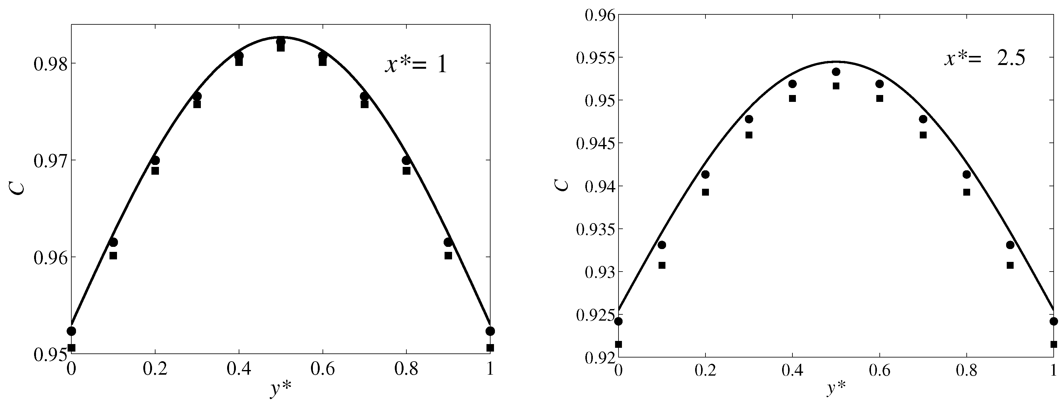
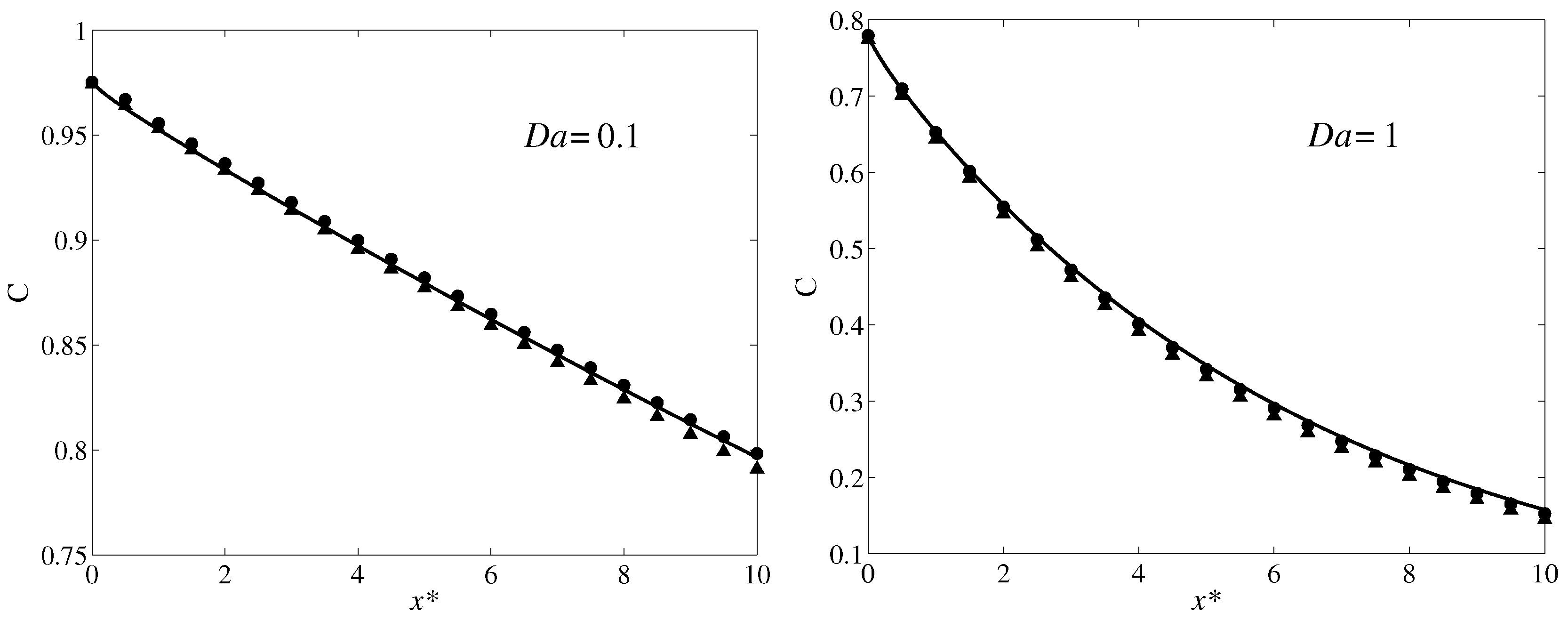
In the numerical simulations, the domain size $101\times 11$ lattice unit spacings for $Pe=10$ and $501\times 11$ lattice unit spacing for $Pe=50$. In Figure 6, the concentration at $x^{-}=0.1,0.25$ is plotted along y-axis with $Pe=10$ and $Da=0.1$ and 1 by different FD method in non-equilibrium extrapolation method. From the figures, we can see that the second order FD in NE method is better than the first order one. The concentration on the top boundary at $x*\in [0,1]$ is shown in Figure 7. From the figures we can see the TRT model with NE method are agree with the analytic solution. And the second order FD is better than the first order FD method.

To demonstrate the accuracy of the non-equilibrium extrapolation method with different finite difference method, the relative error on the top or bottom boundary (BRE) is defined as

$$BRE=\frac{\parallel C_{LB}-C_{analytic}{\parallel }_2}{\parallel C_{analytic}{\parallel }_2}.$$

In

Table 2. The boundary relative error with different $Pe$ number and $Da$ number with H = 10.

Pe	$\mathit{\alpha }$	Da	Finite Difference Method	BRE
10	0.5	0.1	First order FD	3.6532 × ${10}^{-3}$
			Second order FD	1.3245 × ${10}^{-3}$
		1.0	First order FD	1.3200 × ${10}^{-1}$
			Second order FD	3.9277 × ${10}^{-3}$
50	0.2	0.1	First order FD	8.30682 × ${10}^{-3}$
			Second order FD	3.6795 × ${10}^{-3}$
		1.0	First order FD	3.6578 × ${10}^{-2}$
			Second order FD	1.6095 × ${10}^{-2}$

, the relative error on reactive boundary are listed with different $Pe$ number and $Da$ number. From the Table, we can see that the second order finite difference is also better than the first order FD method.

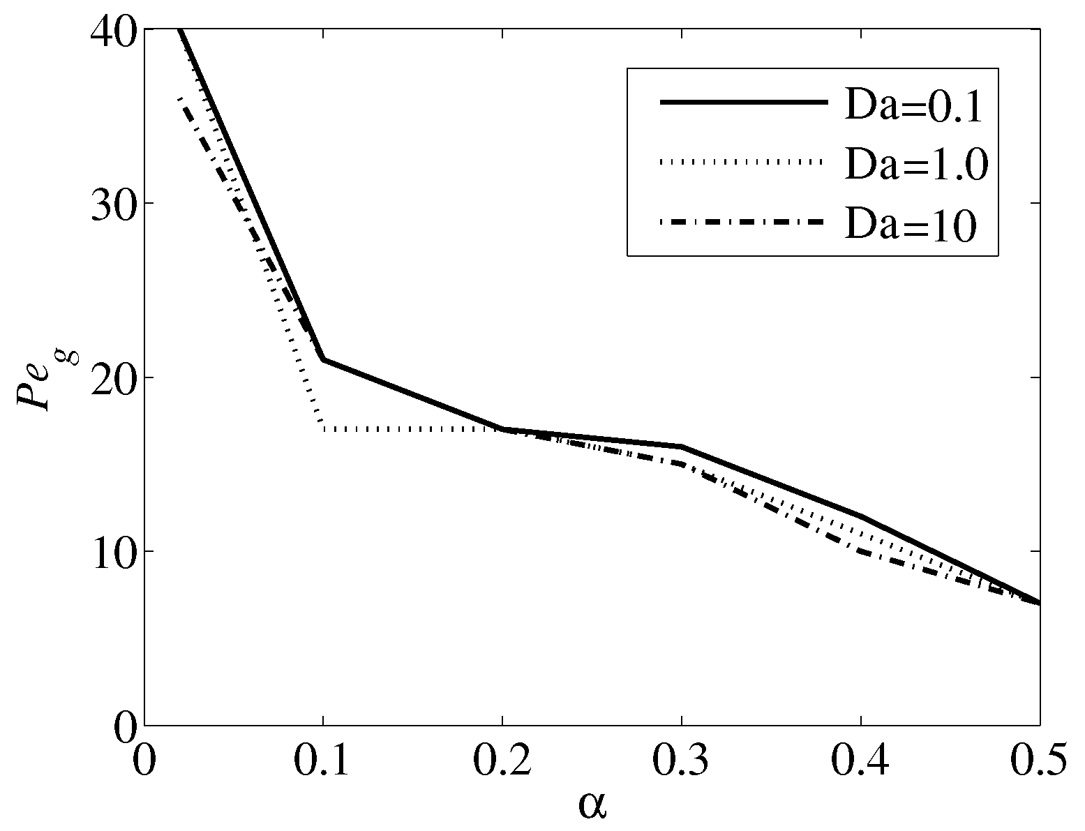
To demonstrate the stability of NE method. We calculate the maximum grid Peclet number $P{e}^{*}$ with different $Da$ and $\alpha$. The width of the channel H is 10. The figures are plotted in Figure 8, and it is shown that the $Da$ number has little influence on the stability. The smaller $\alpha$, the better stability. And maximum $P{e}^{*}$ can reach 40.

6. Conclusions

In this paper, we have proposed a non-equilibrium extrapolation method in TRT model for simulating convection-diffusion flow with a reactive boundary condition. The Dirichlet and mixed boundary conditions have been analyzed. Like the method by Guo, the main point is to obtain the particle distribution function on the boundary. In NE method, it is important to get the physical quantities on the boundary. For the reactive boundary, that is mixed boundary conditions, finite difference is used and it is easy to construct the particle distribution function.

We have verified the accuracy of the NE method with TRT through a comparison with the analytic solution for the convection-diffusion flow in the long channel. From the simulation results, it is in good agreement with the analytic solution. Furthermore, it is of better numerical stability for high Pe numbers, both Dirichlet and mixed boundary conditions, compared with the methods by Ginzburg.

References

- Chen, S.; Doolen, G.D. Lattice Boltzmann method for fluid flows. Ann. Rev. Fluid Mech. 1998, 30, 329–364. [Google Scholar] [CrossRef] [Green Version]
- Liang, H.; Li, Y.; Chen, J.X.; Xu, J.G. Axisymmetric lattice Boltzmann model for multiphase flows with large density ratio. Int. J. Heat Mass Transf. 2019, 130, 1189–1205. [Google Scholar] [CrossRef] [Green Version]
- Du, R.; Sun, D.K.; Shi, B.C.; Chai, Z.H. Lattice Boltzmann model for time sub-diffusion equation in Caputo sense. Appl. Math. Comput. 2019, 358, 80–90. [Google Scholar] [CrossRef]
- Du, R.; Liu, Z.X. A lattice Boltzmann model for the fractional advection-diffusion equation coupled with incompressible Navier-Stokes equation. Appl. Math. Lett. 2020, 101, 106074. [Google Scholar]
- Warren, P.B. Electroviscous transport problems via lattice-Boltzmann. Int. J. Mod. Phys. C 1997, 8, 889–898. [Google Scholar] [CrossRef]
- Békri, S.; Thovert, J.F.; Adler, P.M. Dissolution and Deposition in Fractures. Eng. Geol. 1997, 48, 283–308. [Google Scholar] [CrossRef]
- Szymczak, P.; Ladd, A.J.C. Wormhole formation in dissolving fractures. J. Geophys. Res. 2009, 114, B06203. [Google Scholar] [CrossRef] [Green Version]
- Kang, Q.J.; Lichtner, P.C.; Viswanathan, H.S.; Abdel-Fattah, A.I. Pore Scale Modeling of Reactive Transport Involved in Geologic CO2 Sequestration. Transp. Porous Med. 2010, 82, 197–213. [Google Scholar] [CrossRef] [Green Version]
- Yan, Z.F.; Yang, X.F.; Li, S.L.; Hilpert, M. Two-relaxation-time lattice Boltzmann method and its application to advective-diffusive-reactive transport. Adv. Water Resour. 2017, 109, 333–342. [Google Scholar] [CrossRef]
- Ge, W.; Chang, Q.; Li, C.X.; Wang, J.W. Multiscale structures in particle-fluid systems: Characterization, modeling, and simulation. Chem. Eng. Sci. 2019, 198, 198–223. [Google Scholar] [CrossRef]
- Yu, C.; Deng, A.L.; Ma, J.J.; Cai, X.Q.; Wen, C.C. Semi-analytical solutions for two-dimensional convection-diffusion-reactive equations based on homotopy analysis method. Environ. Sci. Pollut. Res. 2018, 25, 34720–34729. [Google Scholar] [CrossRef]
- Ziegler, D.P. Boundary conditions for lattice-Boltzmann simulations. J. Stat. Phys. 1993, 71, 1171–1177. [Google Scholar] [CrossRef]
- Ladd, A.J.C. Numerical simulations of particulate suspensions via a discretized Boltzmann equation Part I. Theoretical foundation. J. Fluid Mech. 1994, 271, 271–285. [Google Scholar] [CrossRef] [Green Version]
- Kang, Q.; LichtnerI, P.C.; Zhang, D. Lattice Boltzmann pore-scale model for multicomponent reactive transport in porous media. J. Geophys. Res. 2006, 111, B05203. [Google Scholar] [CrossRef]
- Verberg, R.; Ladd, A.J.C. Lattice-Boltzmann model with sub-grid scale boundary conditions. Phys. Rev. Lett. 2000, 84, 2148–2151. [Google Scholar] [CrossRef]
- Bouzidi, M.; Firdaouss, M.; Lallemand, P. Momentum Transfer of a Boltzmann-Lattice Fluid with Boundaries. Phys. Fluids 2001, 13, 3452–3459. [Google Scholar] [CrossRef]
- Ginzburg, I.; D’humieres, D. Multireflection boundary conditions for lattice Boltzmann models. Phys. Rev. E 2003, 68, 066614. [Google Scholar] [CrossRef] [Green Version]
- Junk, M.; Yang, Z. A one-point boundary condition for the lattice-Boltzmann method. Phys. Rev. E 2005, 72, 066701. [Google Scholar] [CrossRef] [Green Version]
- Mei, R.W.; Luo, L.S.; Shyy, W. An accurate curved boundary treatment in the lattice Boltzmann method. J. Comput. Phys. 1999, 155, 307–330. [Google Scholar] [CrossRef]
- Ginzburg, I.; D’humieres, D. Local second-order boundary methods for lattice-Boltzmann models. J. Stat. Phys. 1996, 84, 927–971. [Google Scholar] [CrossRef]
- Guo, Z.L.; Zheng, C.G.; Shi, B.C. An extrapolation method for boundary conditions in lattice Boltzmann method. Phys. Fluids 2002, 14, 2007–2010. [Google Scholar] [CrossRef]
- Chun, B.; Ladd, A.J.C. Interpolated boundary condition for lattice-Boltzmann simulations of flows in narrow gaps. Phys. Rev. E 2007, 75, 066705. [Google Scholar] [CrossRef] [Green Version]
- Yin, X.W.; Zhang, J.F. An improved bounce-back scheme for complex boundary conditions in lattice Boltzmann method. J. Comput. Phys. 2012, 231, 4295–4303. [Google Scholar] [CrossRef]
- Ginzburg, I. Equilibrium-type and link-type lattice Boltzmann models for generic advection and anisotropic-dispersion equation. Adv. Water Res. 2005, 28, 1171–1195. [Google Scholar] [CrossRef]
- Zhang, T.; Shi, B.C.; Guo, Z.; Chai, Z.H.; Lu, J. General bounce-back scheme for concentration boundary condition in the lattice-Boltzmann method. Phys. Rev. E 2012, 85, 016701. [Google Scholar] [CrossRef]
- Ginzburg, I. Consistent lattice Boltzmann schemes for the Brinkman model of porous flow and infinite Chapman-Enskog expansion. Phys. Rev. E 2008, 77, 066704. [Google Scholar] [CrossRef]
- Silva, G.; Semiao, V. First- and second-order forcing expansions in a lattice Boltzmann method reproducing isothermal hydrodynamics in artificial compressibility form. J. Fluid Mech. 2012, 698, 282–303. [Google Scholar] [CrossRef]
- Verberg, R.; Ladd, A.J.C. Simulation of low-Reynolds-number flow via a time-independent lattice-Boltzmann method. Phys. Rev. E 1999, 60, 3366–3373. [Google Scholar] [CrossRef]
Figure 1.
Concentration along the transverse (y) direction at and ; the parameter . Each panel shows results from numerical simulations for a channel width (solid symbols), with different implementations of the boundary conditions: (a) Anti-Bounce-Back (ABB), (b) 2nd-order Multi-Reflection (2nd), (c) 3rd-order Multi-Reflection (3rd), (d) Extrapolation of the non-equilibrium distribution (NE). The solid symbols indicate different displacements () of the left channel wall from the nearest fluid nodes: (squares), (triangles), (circles), and (diamonds). The exact solution is shown by the solid line.
Figure 2.
Centerline concentration along the transverse (y) direction at and ; the parameter . Numerical simulations for a channel width , with different implementations of the boundary conditions, are compared with the exact solution (solid line): 2nd-order MR (triangles), 3rd-order MR (circles), and extrapolation of the NE distribution (diamonds). The offset in the channel was in each case.
Figure 3.
Centerline concentration () for a channel width at (left) and (right); at and at . The symbols indicate the different implementation of the boundary conditions, as indicated in the legend, and the solid line is the analytic solution.
Figure 4.
The maximum grid Péclet number, , obtained with different implementations of the boundary conditions. The stable region (below the line) is illustrated as a function of (4).
Figure 5.
Illustration of the non-equilibrium extrapolation (NE) boundary condition [21]. The thick solid line indicates the boundary between solid (open circles) and fluid (solid squares) domains. The boundary conditions are evaluated at the intersections of the velocity vectors (for example ) and the boundary surface (solid circles).
Figure 6.
Concentration along y-axis at different x with Pe = 10, Da = 0.1 and H = 10. The line is the analytic solution, ‘▴’ is by the first order FD and ‘•’ is by the second order FD.
Figure 7.
Concentration on the top boundary at . The line is the analytic solution, ’▴’ is by the first order FD and ‘•’ is by the second order FD.
Figure 8.
The maximum grid Pe number corresponding to with different Da number by first order FD method.