Structure Functions of Pseudo Null Curves in Minkowski 3-Space


1
Department of Mathematics, Northeastern University, Shenyang 110004, China
2
Department of Mathematics, Kyungpook National University, Daegu 41566, Korea
*
Author to whom correspondence should be addressed.
Mathematics 2020, 8(1), 75; https://0-doi-org.brum.beds.ac.uk/10.3390/math8010075
Submission received: 4 November 2019
/
Revised: 14 December 2019
/
Accepted: 16 December 2019
/
Published: 3 January 2020
(This article belongs to the Special Issue Differential Geometry of Spaces with Structures)
Abstract
:In this work, the embankment surfaces with pseudo null base curves are investigated in Minkowski 3-space. The representation formula of pseudo null curves is obtained via the defined structure functions and the k-type pseudo null helices are discussed completely. Based on the theories of pseudo null curves, a class of embankment surfaces are constructed and characterized by the structure functions of the pseudo null base curves.
1. Introduction
With the development of the theory of relativity, geometers and researchers often extend some topics in classical differential geometry of Riemannian manifolds to those of semi-Riemannian manifolds, especially to Lorentz–Minkowski manifolds. However, due to the causal character of vectors in Lorentz–Minkowski space, some problems become a little strange and different, especially the ones related to lightlike (null) vectors, such as null curves, pseudo null curves, B-scrolls and the marginally trapped surfaces and so on.
It is well known that a space curve is called a helix if its tangent vector makes a constant angle with a fixed direction and it is called a slant helix if its principal normal vector makes a constant angle with a fixed direction [1]. The helix and the slant helix play important roles in the curve theory, and they can be applied into the science of biology and physics etc., such as analyzing the structure of DNA and characterizing the motion of particles in a magnetic field [2]. Due to these fascinating applications, the helix and the slant helix have been discussed widely, not only in the Euclidean space, but also in the Lorentz–Minkowski space [3,4]. Recently, one of the authors investigated the representation formula of null curves via the defined structure functions [5,6] and the null helix and k-type null slant helices in Minkowski four-space were discussed in [6]. Motivated by those ideas, in the second part of this paper, the pseudo null curves are represented by the new defined structure functions, at the same time, the k-type pseudo null helices are defined and characterized by the structure functions in the third part.
Naturally, the surface theory can also be generalized into the Lorentz–Minkowski space. In surface theory, there exists an important class of surfaces, called ruled surfaces, which can be applied in computer aided geometric designs (CAGD), surface approximations and tool path planning, etc. The embankment surfaces as the envelope of cones are just formed by two ruled surfaces with the same base curves [7]. Combining the theories of pseudo null curves, a kind of embankment surface, with pseudo null base curves, are discussed in the fourth part of this work.
Throughout this paper, all the geometric objects under consideration are smooth and all surfaces are connected unless otherwise stated.
2. Representation Formula of Pseudo Null Curves
A Minkowski three-space is provided with the standard flat metric given by
in terms of the natural coordinate system . Recall that a vector v is spacelike, timelike and lightlike (null), if or , and , , respectively. The norm of v is defined by . For any two vectors , , their exterior product is given by
where is an orthogonal basis in . An arbitrary curve is spacelike, timelike or lightlike if all of its velocity vectors are spacelike, timelike or lightlike. At the same time, a surface is said to be timelike, spacelike or lightlike if all of its normal vectors are spacelike, timelike or lightlike, respectively [8]. Furthermore, the spacelike curves in can be classified into the first and the second kind of spacelike curves and the pseudo null curves according to their principal normal vectors are spacelike, timelike and lightlike, respectively. Among of them, the pseudo null curves are defined as following.
Definition 1
([9]). A spacelike curve framed by Frenet frame in is called a pseudo null curve, if its principal normal vector β and binormal vector γ are linearly independent null vectors.
Remark 1.
The pseudo null lines are excluded from consideration throughout this paper.
Proposition 1
([9]). Let be a pseudo null curve parameterized by arc-length s, i.e., . Then there exists a unique Frenet frame , such that
where and In sequence, is called the tangent, principal normal and binormal vector field of , respectively. The function is called the curvature function.
Remark 2.
In some research papers for pseudo null curves such as [9], the function is also called torsion function. Throughout the paper, the pseudo null curves are parameterized by arc-length s.
The cone curves on and null curves in are described by the defined structure functions in [5,10], respectively. Motivated by them, the pseudo null curves in can also be characterized.
First, we write , since is a unit spacelike vector, then Without loss of generality, we can assume
where and are non-constant functions of arc-length s. Then
Therefore, the pseudo null curve can be written as
Furthermore, through direct calculations, we have
Due to , we get
Solving the above differential Equation (4), we get
Proposition 2.
Let be a pseudo null curve in . Then can be written as
where are non-constant functions and they satisfy
Definition 2.
The functions and in Proposition 2 are called structure functions of the pseudo null curve .
Proposition 3.
Let be a pseudo null curve in . Then the curvature function of and its structure function are related by
Proof of Proposition 3.
According to Equation (3), through some calculations, we have
Meanwhile, from the Frenet formula in Equations (1) and (2), through direct calculations, we can get the representations of and . Then, according to Proposition 3, by solving a differential equation system derived by , it is not difficult to get the representation of . Thus, we have the following conclusion.
Proposition 4.
Let be a pseudo null curve in . Then the Frenet frame of can be represented by the structure functions as
where and they are related by , and .
In what follows, we will be concerned with the pseudo null curves with constant curvatures.
Theorem 1.
Let be a pseudo null curve in . If the curvature function is constant, then the structure functions can be written as
- 1.
- when
- 2.
- when
Proof of Theorem 1.
Let the curvature function is constant c, from Equation (6), we have
Case 1: . It is easy to get . By the parameter transformation , where is a constant, we can omit the integration constant here, then . Furthermore, from Equation (5) we have
By an appropriate transformation, we can let . Thus, we have
Case 2: . Similar to the proving procedure in Case 1, we can get and This completes the proof. □
From Proposition 2 and Theorem 1, the following conclusion can be achieved easily through simple integrations [11].
Theorem 2.
Let be a pseudo null curve with constant curvature in . Then can be written as
- 1.
- when
- 2.
- when
3. k-Type Pseudo Null Helices
In this section, we define the k-type pseudo null helices and investigate their properties.
Definition 3
([6]). Let be a pseudo null curve with Frenet frame . If there exists a non-zero constant vector field V such that (respectively, is a constant for all , then is said to be a k-type (k=1,2,3) pseudo null helix and V is called the axis of .
Remark 3.
If the tangent vector α, principal normal vector β or the binormal vector γ of is a constant vector, then every fixed direction V satisfies the above definition. Throughout this paper, we assume this situation never happens.
Let V be the axis of a k-type pseudo null helix . Then V can be decomposed by
where are differentiable functions of arc-length s. Thus
3.1. One-Type Pseudo Null Helix
Theorem 3.
Any pseudo null curve is a one-type pseudo null helix in .
Proof of Theorem 3.
Based on the definition of one-type pseudo null helix, we have
where is a non-zero constant. Differentiating Equation (9) with respect to s, we get
From Equation (8), the curvature is an arbitrary function of arc-length s, together with Equations (9) and (10), we get
where
Conversely, if is an arbitrary function, we can define a vector field V as
Then, we have and . This completes the proof. □
As a consequence of Theorem 3, we have
Corollary 1.
Let be a one-type pseudo null helix. Then the axis V is spacelike and it can be read as
or it can be represented by the structure function as
where and .
3.2. Two-Type Pseudo Null Helix
Theorem 4.
There does not exist two-type pseudo null helix in .
Proof of Theorem 4.
3.3. Three-Type Pseudo Null Helix
Theorem 5.
Let be a pseudo null curve in . Then is a three-type pseudo null helix if and only if its curvature satisfies
Explicitly, the curvature function can be written as
- 1.
- 2.
- 3.
where and .
Proof of Theorem 5.
Based on the definition of three-type pseudo null helix, we have
where is a non-zero constant. Then, by taking derivative on both sides of Equation (13), we get
Substituting into the third equation of Equation (8), we know
Let , then Equation (16) can be rewritten by
Since the curve is a planar curve when is a constant [11], then for a three-type pseudo null helix. Solving the following differential equation
we have
Solving the differential Equation (17), we get three cases as follows.
Case 1: . It is easy to get
Taking it into Equation (15), we have
Case 2: . By direct calculations, we obtain
Substituting it into Equation (15), we get
Case 3: . After direct calculations, we obtain
Taking it into Equation (15), we have
Conversely, when satisfies one of the following conditions, we can choose an appropriate constant vector V as
- for
- for
- for
Obviously, for each case, we have and . □
As a consequence of Theorem 5, we have
Corollary 2.
Let be a three-type pseudo null helix. Then the axis V can be read as
- 1.
- when , the axis V is lightlike. And
- 2.
- when , the axis V is timelike. And
- 3.
- when , the axis V is spacelike. And
where .
From Theorem 5 and Proposition 3, we have
Corollary 3.
Let be a three-type pseudo null helix. Then the structure functions of can be written as
- 1.
- when ;
- 2.
- when ;
- 3.
- when ,
where .
Proof of Corollary 3.
When , by the parameter transformation , (), we can let , i.e., . From Equation (6), we know then . Without loss of generality, we can put , then Furthermore, from Equation (5), we have
By an appropriate transformation, we can let . Thus,
Similarly, when and , by the parameter transformation, we can get
Solving the above two differential equations analogous to the first case, i.e., , we can get the other two conclusions easily. □
Substituting the conclusions obtained in Corollary 3 to the representation formula shown by Proposition 2, after direct integrations, we have
Corollary 4.
Let be a three-type pseudo null helix. Then can be written as
- 1.
- for ;
- 2.
- for ;
- 3.
- for ,
where .
4. Embankment Surfaces with Pseudo Null Base Curves
Given a one parameter family of regular implicit surfaces The intersection curve of two neighbored surfaces and fulfills the two equations and We consider the limit for and get
which motivates the following definition.
Definition 4
([7]). Let be a one parameter family of regular implicit -surfaces. The surface defined by the two equations
is called an envelope of the given family of surfaces.
Definition 5
([7]). Let be a regular space curve and with The envelope of the one parameter family of cones
is called an embankment surface and Γ its base curve.
Remark 4
([7]). In fact, the embankment surface in above definition is consisted by two ruled surfaces which can be represented as follows
with and are intersection points of the circle and the line
Motivated by the generating process of embankment surfaces, we can construct a kind of embankment surface in based on a pseudo null curve as follows.
Definition 6.
Let be a pseudo null curve framed by in and . Then the surface partner
is called an embankment surface and its base curve.
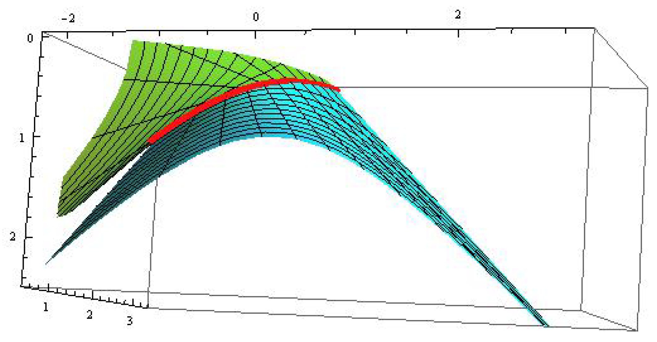
Example 3.
Consider an embankment surface with a pseudo null base curve of curvature (see Figure 6).
From Proposition 3, the structure functions of are
Then, by Proposition 2, we know
From Proposition 4, the principal normal vector β and binormal vector γ of are and
Combining the conclusions obtained in Section 3, when the base curve of an embankment surface is a three-type pseudo null helix, we have
Theorem 6.
Let be an embankment surface with three-type pseudo null helix as its base curve. Then can be classified as
- 1.
- when , where
- 2.
- when , where
- 3.
- when , where
where ,
Proof of Theorem 6.
From Corollary 4, when , the pseudo null curve . According to Equation (1), we obtain
where are constants and related by Through some direct calculations, we obtain Therefore
Similar to the first case, we can get the other two results, their explicit proofs are omitted here. □
Example 4.
Consider the embankment surfaces with a three-type pseudo null helix stated in Example 2 as its base curve.
Remark 5.
The idea to study pseudo null curves by constructing structure functions can be extended into other space–times and space forms, such as the hyperbolic space–time and de-Sitter space–time. At the same time, the structure functions of pseudo null curves defined in this work can also be applied to some other submanifolds, such as the canal (tube) submanifold, translation submanifold, product submanifold and rotation submanifold, which play important roles in CAD (CAGD).
Author Contributions
J.Q., J.L. and X.T. set up the problem and computed the details. Y.H.K. checked and polished the draft. All authors have read and agreed to the published version of the manuscript.
Funding
The first author was supported by NSFC (No.11801065) and the fourth author was supported by the National Research Foundation of Korea (NRF) grant funded by the Korea Government (MSIP) (2016R1A2B1006974).
Acknowledgments
We thank the referee for the careful review and the valuable comments to improve the paper.
Conflicts of Interest
The authors declare no conflict of interest.
References
- Izumiya, S.; Takeuchi, N. New special curves and developable surfaces. Turk J. Math. 2004, 28, 153–163. [Google Scholar]
- Lucas, A.A.; Lambin, P. Diffraction by DNA, carbon nanotubes and other helical nanostructures. Rep. Prog. Phys. 2005, 68, 1181–1249. [Google Scholar] [CrossRef]
- Ferrandez, A.; Gimenez, A.; Lucas, P. Null generalized helices in Lorentz–Minkowski spaces. J. Phys. A Math. Gen. 2002, 35, 8243–8251. [Google Scholar] [CrossRef]
- Kula, L.; Ekmekci, N.; Yayli, Y.; Ilarslan, K. Characterizations of slant helices in Euclidean 3-space. Turk J. Math. 2010, 34, 261–273. [Google Scholar]
- Qian, J.H.; Kim, Y.H. Directional associated curves of a null curve in . Bull. Korean Math. Soc. 2015, 52, 183–200. [Google Scholar] [CrossRef]
- Qian, J.H.; Kim, Y.H. Null helix and k-type null slant helices in . Revista De La Union Math. Argentina 2016, 57, 71–83. [Google Scholar]
- Hartmann, E. Geometry and Algorithms for Computer Aided Design; Darmstadt University of Technology: Darmstadt, Germany, 2003; pp. 115–118. [Google Scholar]
- Inoguchi, J.; Lee, S. Null curves in Minkowski 3-space. Int. Electron. J. Geom. 2008, 1, 40–83. [Google Scholar]
- Nesovic, E.; Ozturk, U.; Ozturk, E.B.K. On k-type pseudo null Darboux helices in Minkowski 3-space. J. Math. Anal. Appl. 2016, 439, 690–700. [Google Scholar] [CrossRef]
- Liu, H.; Meng, Q. Representation formulas of curves in a two- and three-dimensional lightlike cone. Result. Math. 2011, 59, 437–451. [Google Scholar] [CrossRef]
- Walrave, J. Curves and Surfaces in Minkowski Space. Ph.D. Thesis, Faculteit Der Wetenschappen, Leuven, Belgium, 1995; pp. 20–21. [Google Scholar]
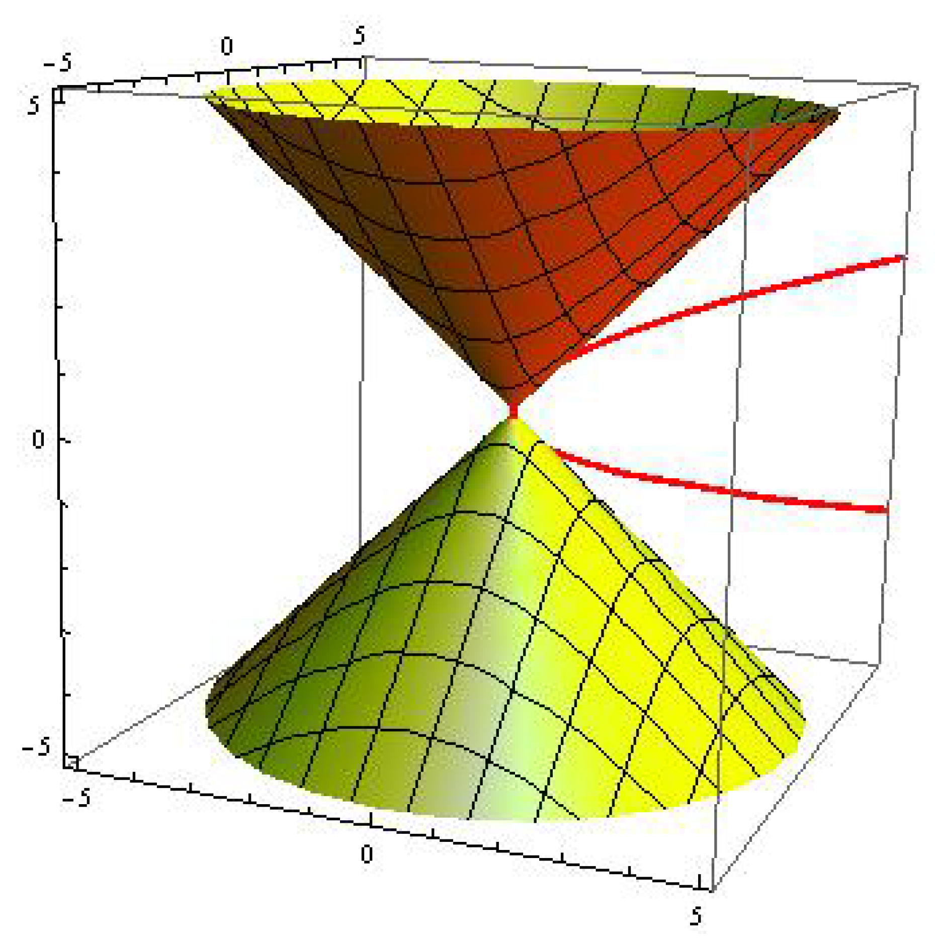
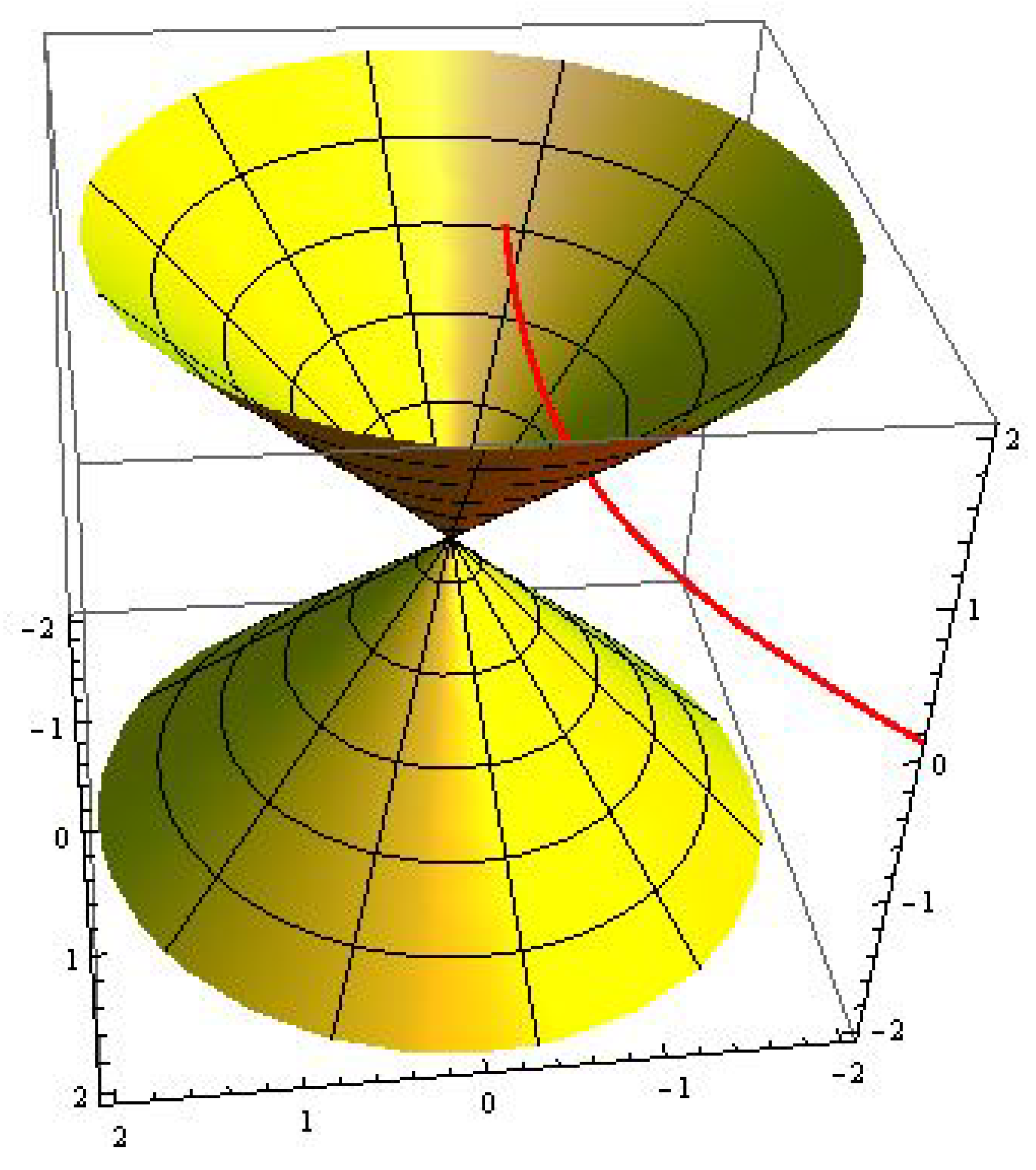
Figure 1.
shown with cone.

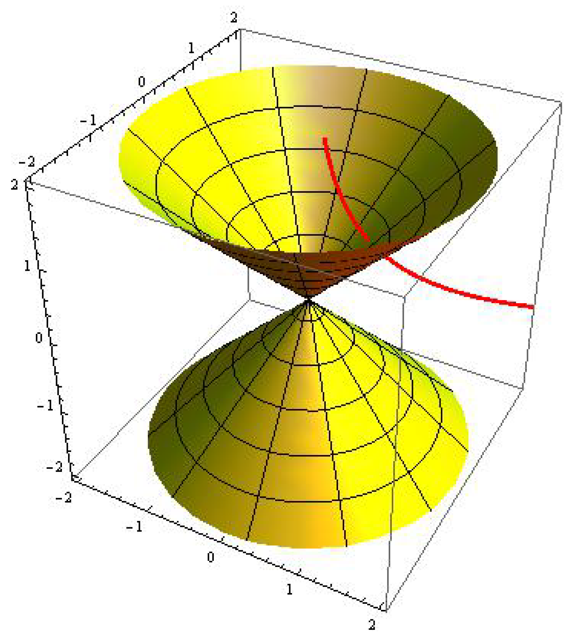
Figure 2.
shown with cone.

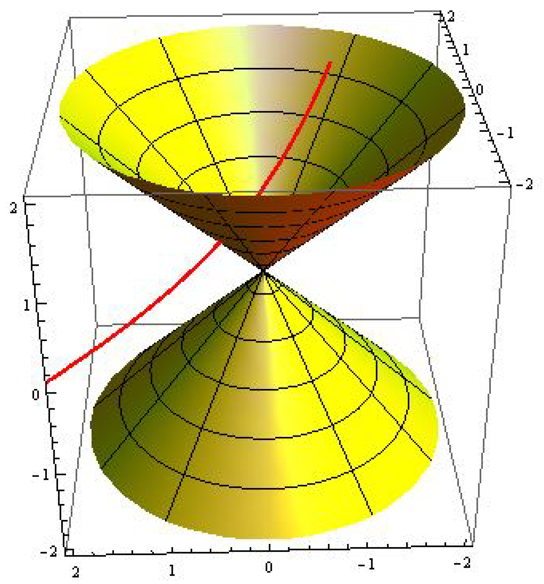
Figure 3.
shown with cone.

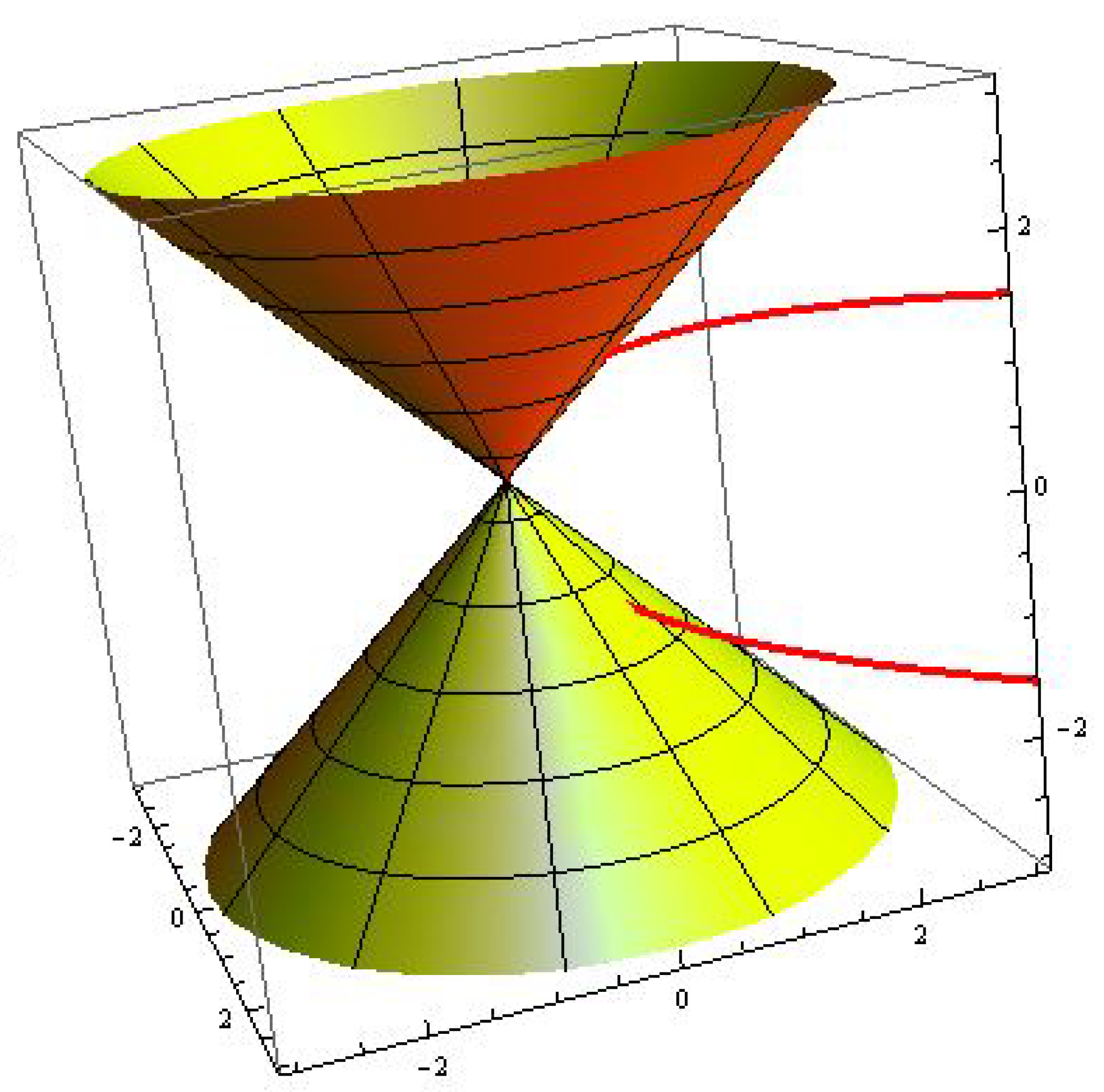
Figure 4.
shown with cone.

Figure 5.
shown with cone.

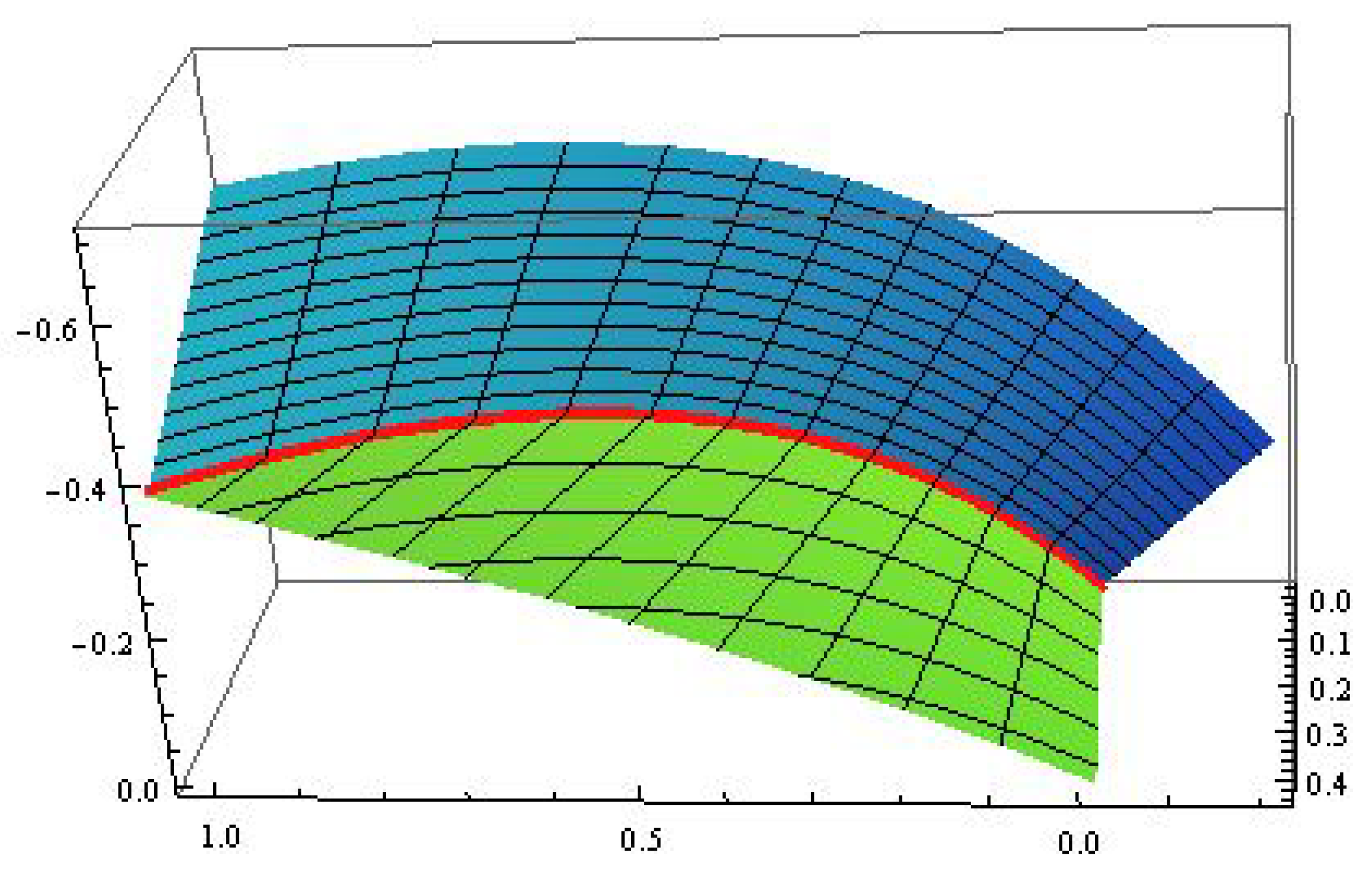
Figure 6.
Embankment surface with the red base curve .

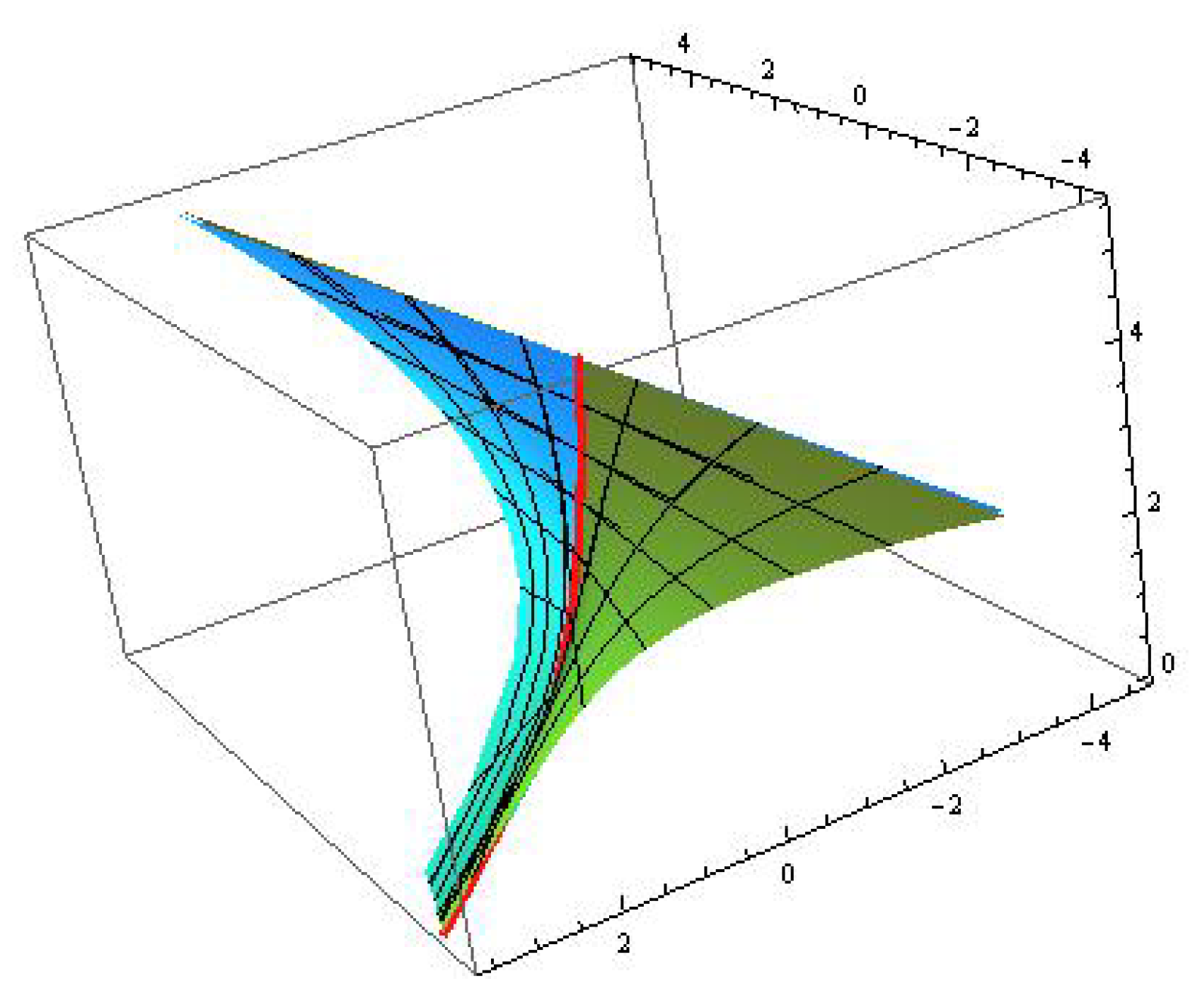
Figure 7.
Embankment surface in 1.

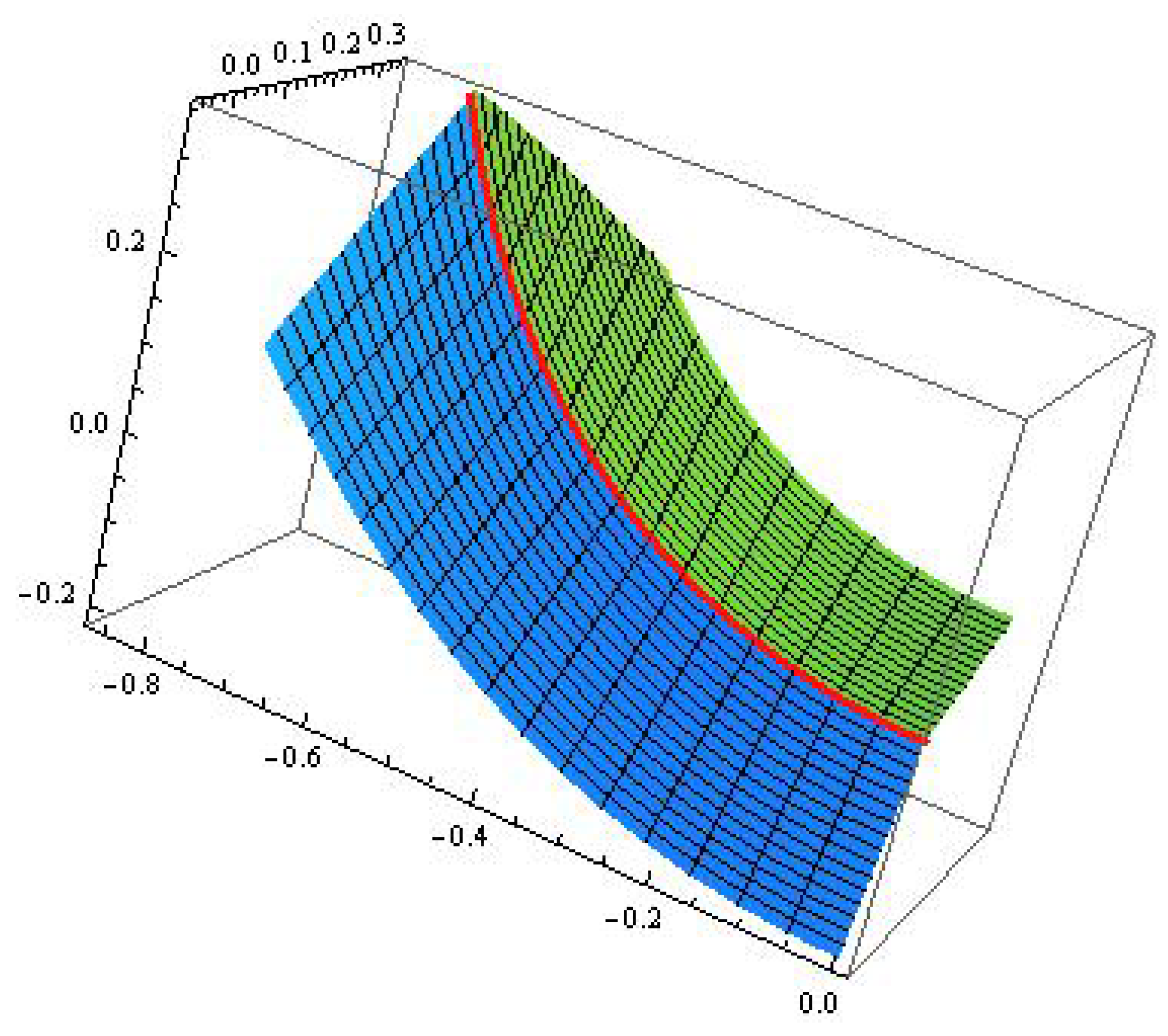
Figure 8.
Embankment surface in 2.

Figure 9.
Embankment surface in 3.

© 2020 by the authors. Licensee MDPI, Basel, Switzerland. This article is an open access article distributed under the terms and conditions of the Creative Commons Attribution (CC BY) license (http://creativecommons.org/licenses/by/4.0/).
Share and Cite
MDPI and ACS Style
Qian, J.; Liu, J.; Tian, X.; Kim, Y.H. Structure Functions of Pseudo Null Curves in Minkowski 3-Space. Mathematics 2020, 8, 75. https://0-doi-org.brum.beds.ac.uk/10.3390/math8010075
AMA Style
Qian J, Liu J, Tian X, Kim YH. Structure Functions of Pseudo Null Curves in Minkowski 3-Space. Mathematics. 2020; 8(1):75. https://0-doi-org.brum.beds.ac.uk/10.3390/math8010075
Chicago/Turabian StyleQian, Jinhua, Jie Liu, Xueqian Tian, and Young Ho Kim. 2020. "Structure Functions of Pseudo Null Curves in Minkowski 3-Space" Mathematics 8, no. 1: 75. https://0-doi-org.brum.beds.ac.uk/10.3390/math8010075
Note that from the first issue of 2016, this journal uses article numbers instead of page numbers. See further details here.