Clustering and Dispatching Rule Selection Framework for Batch Scheduling


Department of Industrial and Management Engineering, Hanyang University, Ansan 15588, Korea
*
Author to whom correspondence should be addressed.
Mathematics 2020, 8(1), 80; https://0-doi-org.brum.beds.ac.uk/10.3390/math8010080
Submission received: 3 December 2019
/
Revised: 27 December 2019
/
Accepted: 29 December 2019
/
Published: 3 January 2020
(This article belongs to the Special Issue Intelligent Optimization in Big Data, Machine Learning and Artificial Intelligence)
Abstract
:In this study, a batch scheduling with job grouping and batch sequencing is considered. A clustering algorithm and dispatching rule selection model is developed to minimize total tardiness. The model and algorithm are based on the constrained k-means algorithm and neural network. We also develop a method to generate a training dataset from historical data to train the neural network. We use numerical examples to demonstrate that the proposed algorithm and model efficiently and effectively solve batch scheduling problems.
1. Introduction
The aim of this study involves developing a framework that schedules batch jobs with identical machines to minimize total tardiness. The objectives of this framework include solving the problem in a short period, solving various batch scheduling problems, and improving performance as more problems are solved. We design a framework based on clustering and classification models because the machine learning approach fits well with the aforementioned goals.
Typical approaches for batch scheduling problems are categorized into heuristic, meta-heuristic, and dispatching rule approaches. The heuristic approach develops an algorithm that is problem-specific. The meta-heuristic approach modifies a meta-heuristic algorithm (e.g., to solve problems). The dispatching rule approach calculates the priority of each job or batch of jobs via a set of predetermined dispatching rules. The jobs are then processed in order of descending priority.
Heuristic and meta-heuristic approaches are usually dependent on the types of problems that are considered [1,2]. Since they are designed for a specific problem, they may yield relatively poor results when applied to different problems, or a substantial modification to the model is necessary before application. Additionally, a relatively long run time is sometimes necessary to yield a schedule using these approaches.
The dispatching rule approach is suitable for the aforementioned goals because it is relatively robust in terms of problem types, and thus can be applied to various problems without substantial modification to yield a schedule quickly. However, this approach occasionally encounters issues in selecting the optimal dispatching rule because it cannot outperform other rules in every scheduling situation [3]. Thus, an optimal universal dispatching rule is absent. Additionally, the optimal rule can change as successive jobs are completed, thereby implying that a dynamic dispatching rule can work better. Several studies developed classification models to select dynamic dispatching rules. For example, Mouelhi-Chibani and Pierreval [3] trained a neural network with dozens of queue state variables to select dispatching rules for flow shop scheduling. Similarly, Shiue [4] developed a support vector machine-based dispatching rule selection model for shop floor control system scheduling. Meanwhile, a few studies developed machine learning model to determine scheduling parameters. Mönch et al. [5] trains a neural network and inductive decision tree to estimate the weight of the ATC (apparent tardiness cost) rule, which consists of two dispatching rules: weighted shortest processing time rule and the least slack rule.
However, there is a paucity of extant studies on developing a dispatching rule selection model for the batch scheduling problem. This requires grouping jobs into batches before applying a dispatching rule. We design a clustering algorithm to group similar jobs under machine capacity constraints and add it to the framework.
The major contents and contributions of this study are as follows. First, we develop a clustering algorithm based on the constrained k-means algorithm to group jobs into batches. The algorithm uses a set of features impacting total tardiness and yields clusters that contain jobs wherein sums of job sizes do not exceed the machine load capacity. Second, we develop a step-by-step method based on the Monte Carlo Markov chain (MCMC) approach to create a training dataset to work with the dispatching rule selection model. Each sample in the dataset represents the virtual queue state via queue state variables (e.g., the number of batches in the queue and maximum processing time of the batches). Subsequently, the samples are attached to the optimal dispatching rule for the particular state. Third, we design a dispatching rule selection model based on neural networks for batch sequencing. Whenever a machine is available, queue state variable values for the current queue state enter the model to yield the optimal dispatching rule.
Section 2 introduces the batch scheduling problem including major assumptions, notations, and an overview of the framework. Section 3 describes methods to generate the training dataset to transform the variables to the queue status variables and to design the dispatching rule selection model. Section 4 discusses the clustering algorithm and application procedure and explains the model deployment process. Section 5 provides illustrative examples to show the application of the proposed model. Section 6 summarizes our conclusions and proposes future research directions.
2. Problem Statement, Notations, and Framework Overview
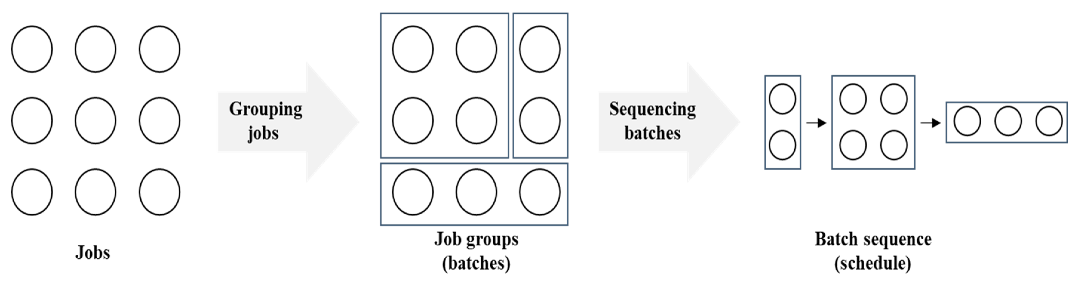
There are jobs to be processed by one of identical machines. Each job is characterized by job characteristics, namely processing time , size , due date , and release time . Jobs are grouped into batches, and a process sequence is determined via a dispatching rule (Figure 1). The former and latter stages are termed as grouping jobs and sequencing batches, respectively [6]. The sum of job sizes in each batch must be equal to or less than the load capacity of a machine. Each batch is processed by a machine as soon as it is available.
The batch processing time denotes the longest processing time among all jobs in the batch [7]. The objective of scheduling involves minimizing total tardiness as follows:
where , , and denote tardiness, completion time, and due date of job , respectively.
The major assumptions are as follows:
- All job characteristics, , of job are known in advance.
- Every job is ready for processing at its release time.
- Neither setup nor rework is assumed.
- Each machine only processes one batch at a time.
- The characteristics data of several historical jobs are available and are sufficient to create a training dataset for the dispatching rule selection model.
Notations used in this study are as follows.
Indices
- Batch index
- Job index
- Time index
- Training sample index
Job characteristics
- Processing time of job
- Size of job
- Due date of job
- Release time of job
- Slack time of job , i.e., the remaining time until due date after finishing the process, at its release time,
- Slack time of job at time ,
Batch characteristics
- Set of job indices in batch
- Processing time of batch ,
Notations for clustering
- Load capacity of a machine
- Vector of job ’s characteristics for grouping purposes,
- Centroid of batch
- Distance between and
Notations for dispatching rule selection
- Dispatching rule for sample
- Number of batches waiting in the queue in sample , for all
- System’s clock time with respect to sample
- Probability mass function of , where either corresponds to processing time (), size (s), slack time (), or release time (r)
- Candidate queue state variable
- Selected queue state variable ,
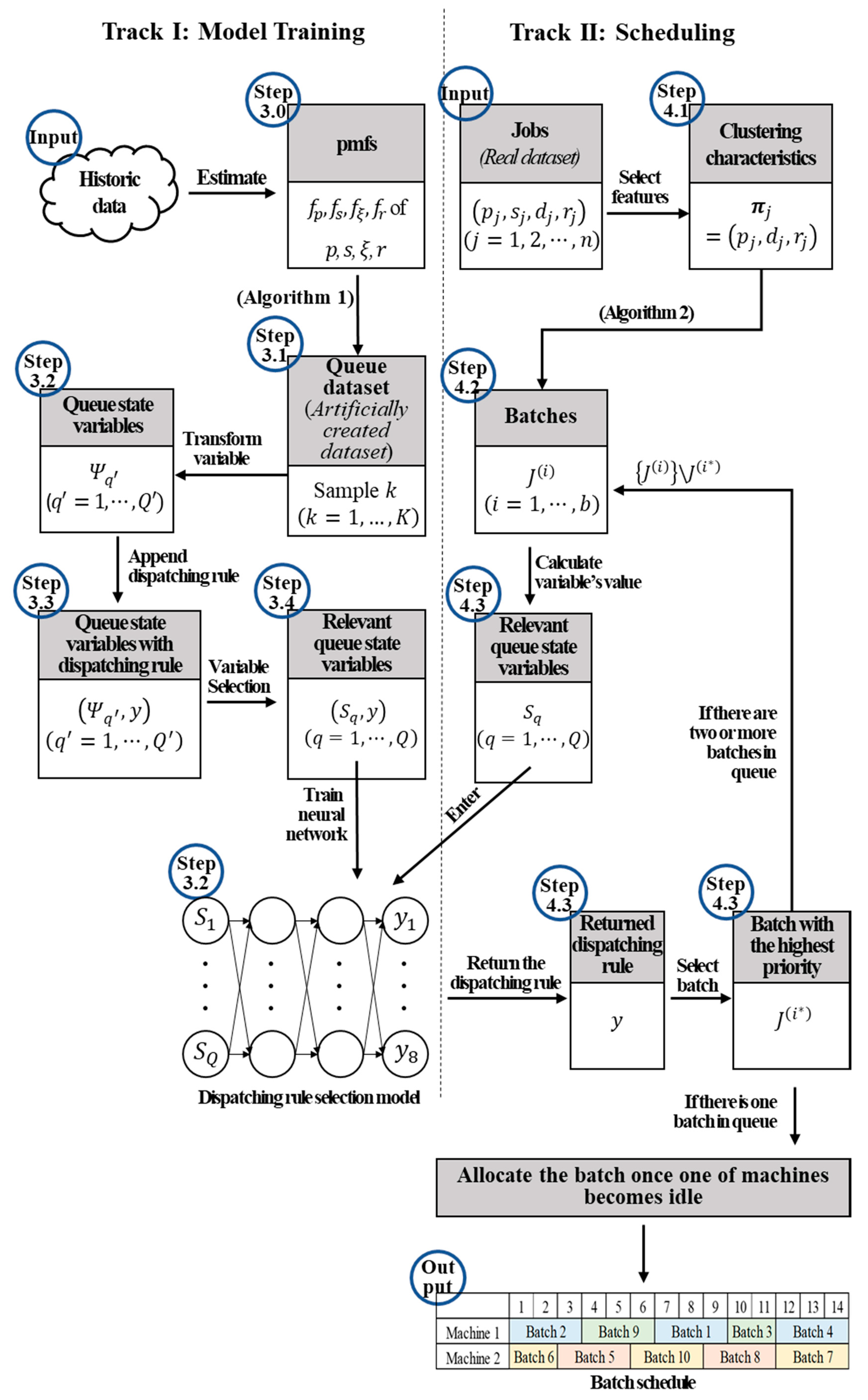
Figure 2 shows the step-by-step process that is used to obtain the set of job batches and the batch sequence for the machines to process. The framework consists of two tracks. Track I is termed as the model training track and is used to build a dispatching rule selection model via a training dataset of batches that is artificially created from historic data. Track II is termed as the scheduling track and is used to group the actual jobs into batches and to determine the processing sequence using the model provided by Track I.
3. Model Training for Dispatching Rule Selection
3.1. Generating the Training Dataset
In this subsection, we introduce the step-by-step method used to create a dataset from historic data of job characteristics. The probability distributions of each job characteristic are calculated, and samples are then created to form a virtual batch dataset. This dataset is then transformed to a more adequate format for training.
Step 3.0: Prepare the probability distributions of job characteristics.
First, the pmfs (probability mass functions) , , , and of processing time (), size (s), slack time (, and release time (r), respectively, are estimated from the historic data based on the relative frequencies as follows:
where and denote the number of jobs that satisfy .
Step 3.1: Create batches in the queue dataset.
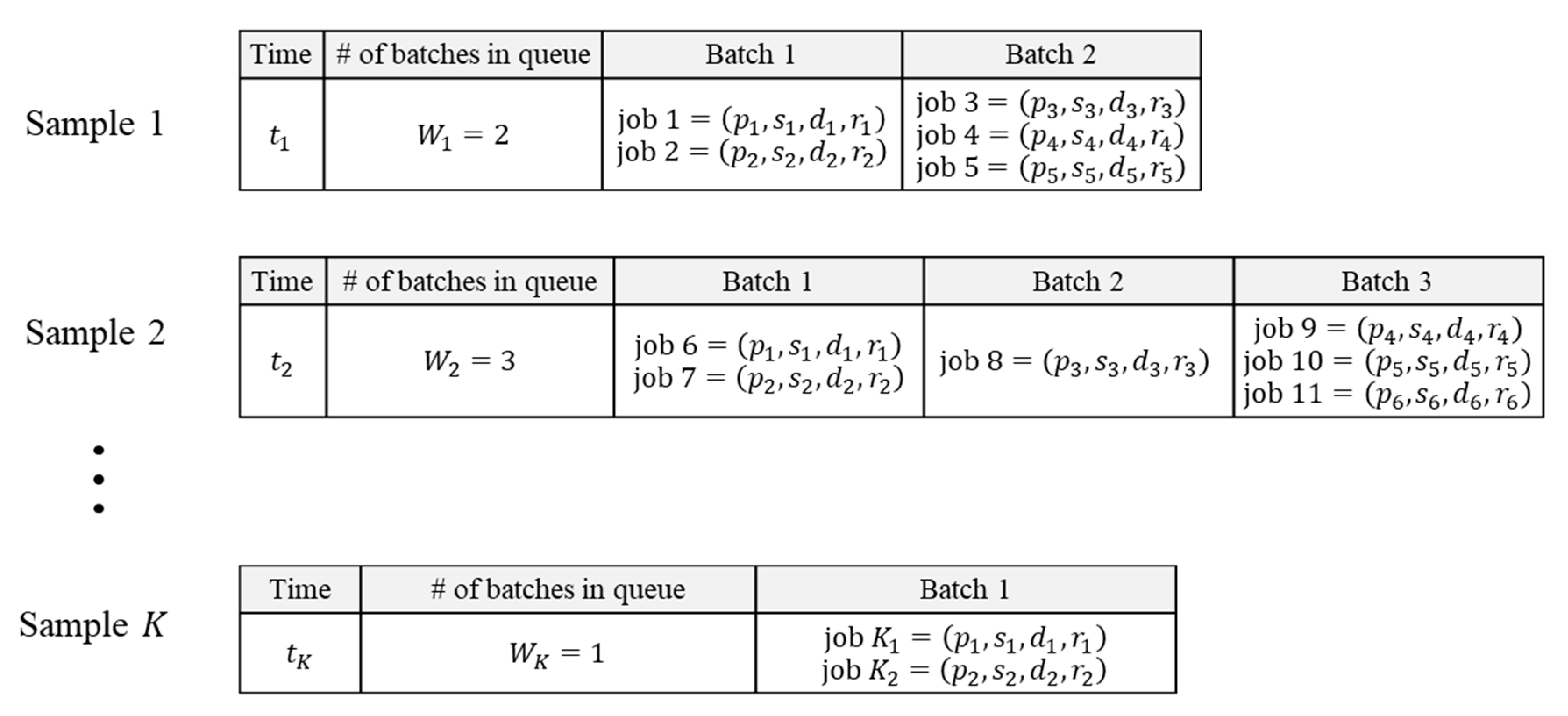
With the pmfs, total samples are generated where sample exhibits batches and each batch consists of one or more jobs characterized by job characteristics . Specifically, is arbitrarily picked in the interval , where . Next, the system’s clock time of sample should exceed any release times of jobs in the queue (). It also must be smaller than the maximum remaining processing time, and this is as follows. There are currently batches that remain in the queue, and thus it is inferred that batches are processed and the mean processing time of existing batches in the queue corresponds to . Therefore, is arbitrarily picked and satisfies .
Figure 3 shows a typical example of a set of samples generated from estimated pmfs. The set of artificial samples is termed as the queue dataset because the batches in each sample wait in the queue to be processed.
Note: It is necessary to exercise caution when more than one job is created in a batch. When a job is sampled, then the next job should be “similar” in terms of its job characteristics to that previously sampled because batches contain “similar” jobs. This is performed by using the following conditional pmfs as follows:
where denotes one of the variables , denotes the previously generated job’s characteristic, denotes the number of clusters containing jobs satisfying and , and denotes the number of clusters that contain at least one job wherein corresponds to .
Algorithm 1 shows the generation process of the queue dataset explained above.
| Algorithm 1. Queue dataset generation algorithm | |
| Input | , , , , , , , , |
| Procedure | For ( to ) Do { |
| Select from at random | |
| Initialize batch as an empty set for | |
| For ( to ) Do { | |
| job_size_sum = 0 | |
| /* First job generation */ | |
| , , , | |
| Append job 1 = (, , , ) to batch | |
| Increase job_size_sum by | |
| /* job generation */ | |
| While (True) Do { # while capacity constraint is satisfied | |
| , , , | |
| If (job_size_sum + ) Do { | |
| break} | |
| Increase job_size_sum by | |
| Append job = (, , , ) to batch | |
| Increase by 1} | |
| Append batch to sample in queue dataset} | |
| is randomly selected from [, ]} | |
| Output | Queue dataset |
Step 3.2: Transform the variables.
Each sample of the queue dataset contains the values of system time () and job characteristics (). It is necessary to transform them into the values representing the status of batches in the queue, as this facilitates improved training for the machine learning model. We introduce queue state variables, , with which the current status of the queue is well defined and contributes to determining the optimal dispatching rule [3]. Queue state variables are defined by in extant studies [3,4,8] as listed in Table 1.
Variables to represent the batch state (e.g., number of batches and processing times of the batch) while to describe the job state (e.g., slack time of jobs). Moreover, the queue dataset consists of 21 queue state variables along with system time.
Step 3.3: Assign the optimal dispatching rule to each training sample.
This step determines the optimal dispatching rule for sample of the batches in the queue dataset. The dispatching rules in Table 2 are considered.
We apply each rule to the batches in each queue dataset sample and then determine the optimal rule to minimize total tardiness. This is appended to each queue dataset sample and is used as a class label of the dispatching rule selection model.
Step 3.4: Select relevant queue state variables.
This step involves examining the queue state variables and removing those that are not relevant to the dispatching rule, . The relevance of a queue state variable is calculated, and variables with high relevance are selected as inputs in the training. We adopt ANOVA’s (analysis of variance) F-statistics for class-relevance, as suggested by [9]:
where the group denotes a set of samples with the same optimal dispatching rule.
Table 3 shows the structure of the queue dataset that is used as the training dataset for the dispatching rule, where denotes a set of (selected) relevant queue state variables.
3.2. Model Training
We develop a machine learning model that uses the values of the queue state variables to determine the dispatching rule, from which the processing order of actual job batches is derived. We select the artificial neural network because it is widely used and has yielded reliable results in previous research [10]. It should be noted that any type of classification model can be used in place of the neural network model.
Recall that, according to the steps of Section 3.1, values of the queue state variables are calculated from the generated dataset, and the optimal dispatching rule is derived, which gives the minimum tardiness. We use the ANOVA to select the relevant queue state variables , and then () composes one sample of the training dataset that will be an input to the neural network. Therefore, the neural network is trained against the dispatching rule for each given values of the queue state variables.
The neural network in our model exhibits an input layer, an output layer, and two hidden layers. Each node in the input layer corresponds to each queue state variable, and each node in the output layer matches the candidate dispatching rule. The number of nodes in the hidden layers are parameters that should be tuned. We test 45 models with nodes in each hidden layer , where and denote the number of nodes in the first and second hidden layers, respectively, and we select the parameters exhibiting the optimal performance with five-fold cross validation.
4. Clustering Model to Group Jobs
Similar jobs are grouped together to form a group of batches when a set of jobs to be processed are newly entered. Jobs in each batch are simultaneously processed.
4.1. Clustering Model to Group Jobs
When jobs are processed in a batch and not individually, the completion time of the jobs are negatively impacted by the wasted processing time, , and residual machine capacity of batch , . Therefore, minimizing both wasted processing time and residual machine capacity decreases the tardiness of the jobs [11]. Additionally, variance of the jobs’ due dates also increases the tardiness of the jobs. Thus, it is necessary to use the processing time , due date , and release time while grouping the jobs into batches. Specifically, denotes the vector of the job characteristics for clustering and is termed as clustering characteristics. Job size is considered as the clustering constraint.
4.2. Formations of Batches
Grouping jobs is based on the constrained -means clustering algorithm. It consists of three steps, namely the centroid initialization step, job assignment step, and centroid update step as follows:
(i) Centroid initialization step:
The initial number of batches is obtained by dividing the total size of the jobs by the machine capacity (i.e., ), and the centroids for are randomly initialized.
(ii) Job assignment step:
Each job is assigned to the nearest cluster. If there is a cluster that does not satisfy the machine capacity constraints, then one or more jobs in that cluster should be re-assigned. The algorithm identifies a job that is the farthest from the cluster’s centroid to which it belongs (e.g., cluster ), albeit the closest to the next nearest cluster’s centroid, i.e., ). It assigns job to the nearest cluster among those satisfying the capacity constraint, .
(iii) Centroid update step:
The centroid of each cluster is updated.
The job assignment step and centroid update step are repeated until the clustering converges. If the clustering does not converge even after a certain predetermined number of times, then we increase the number of batches by 1, and the procedure is repeated until we have enough number of batches that accommodates all jobs. The following Algorithm 2 summarizes the clustering algorithm described above.
| Algorithm 2. Clustering algorithm for grouping jobs | |
| Input | and for all , maximum iteration number |
| Procedure | /* Centroid initialization step */ |
| # Initialize the number of batches | |
| Select randomly | |
| /* Job assignment step */ | |
| number of iterations = 1 | |
| Until (converged) Do { | |
| If (number of iterations > ) Do { | |
| Iteration = 1 | |
| Increase by 1} | |
| For ( to ) Do { | |
| Assign job to the nearest cluster } | |
| For ( to ) Do { | |
| While Do { | |
| Find job | |
| Assign job to another cluster , where | |
| }} | |
| /* Centroid update step */ | |
| Update as | |
| Increase the number of iterations by 1} | |
| Output | Job clusters (batches) |
The following is an illustrative example of the clustering algorithm to improve the reader’s understanding.
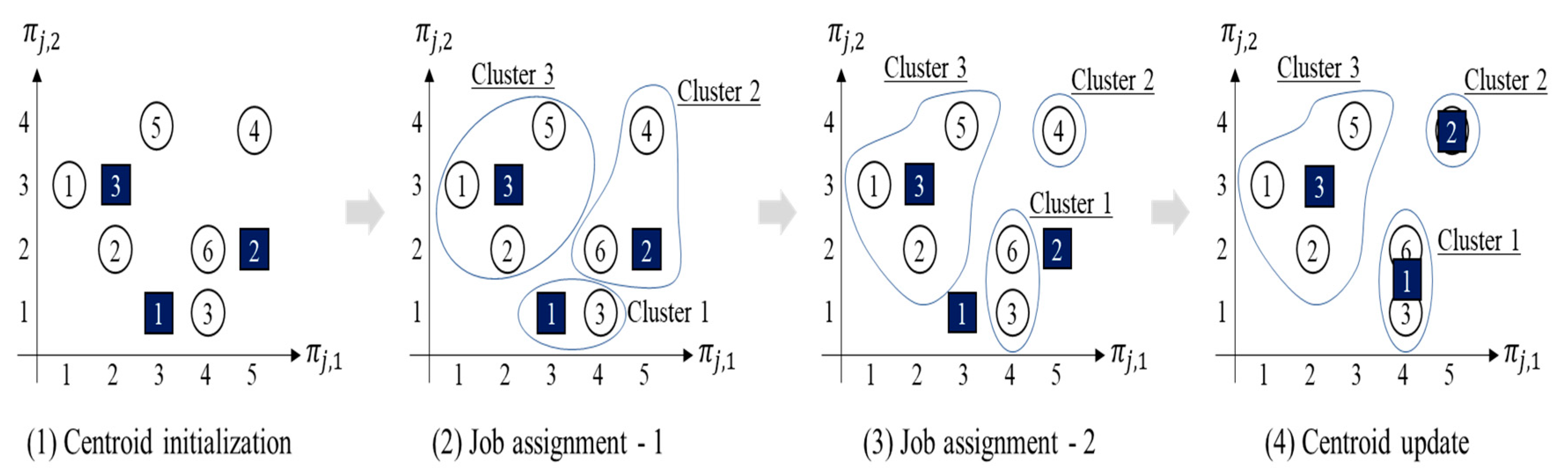
Assume there are six jobs: , , , , , and as depicted in Figure 4. Each job is expressed as a two-dimensional vector for graphical convenience. The job sizes are , , , , , and , and the machine capacity is 4.
- (i)
- Centroid initialization step: Since , we commence with three clusters (i.e., ). Three centroids, namely , , and (black squares in the figure), are randomly generated.
- (ii)
- Job assignment-1: every job is assigned to the nearest cluster. Cluster 1 = {job 3}, cluster 2 = {job 4, 6}, and cluster 3 = {job 1, 2, 5}.
- (iii)
- Job assignment-2: Cluster 2 does not satisfy the capacity constraint since , and either job 4 or job 6 should be reassigned to another cluster. Given that , we select . The total job sizes of cluster 1 and cluster 3 are 1 and 4, respectively; thus, job 6 is reallocated to cluster 1.
- (iv)
- Centroid update: each cluster centroid is updated as , , and .
This process is repeated until the centroid of every batch is not updated any longer.
4.3. Model Deployment
After the jobs are grouped via the proposed clustering model, the rule selection model determines the batch to be processed whenever a machine becomes idle. First, the values of the selected queue state variables are calculated from batches, and the current time is set when the machine becomes idle. Next, the rule selection model selects the proper dispatching rule via the trained neural network. Finally, the selected rule calculates the priority of each batch, determines the highest priority, and processes it with the idle machine. Note that the selected rule may be different from the those selected by human experts because scheduling decisions of human and software models can be different from each other, and thus it is recommended not to rely only on the selected rule but to consider a human expert’s experience for practical usage as suggested in [12].
5. Experiment
This section illustrates the application procedure of the proposed framework to batch scheduling problems to minimize total tardiness where every job is released on the first day. We consider a test case with a small number of jobs and verify the proposed framework’s effectiveness by comparing it with the optimal schedule obtained via exhaustive search. Please refer to [13] for the algorithm to find the optimal solution of small batch scheduling problems.
Additionally, we show the validity of the proposed framework by comparing it with the schedules from single dispatching rules to solve large-scale realistic problems. Based on the experiment, we suggest that the proposed framework determines an optimal schedule for small problems and a better schedule than those obtained via a single dispatching rule for large problems.
5.1. Parameters
We assume that the pmfs and conditional pmfs (cpmfs) of job characteristics are estimated from the historical data listed in Table 4 and Table 5, respectively.
Each cell in Table 5 indicates . For example, the value 0.076 in Table 5 denotes the probability , which denotes that the processing time of a newly generated job corresponds to 2 when the processing time of the previously generated sample corresponds to 1. It should be noted that we do not consider because every job is assumed to be released at once.
For the purpose of training, we first generated a training dataset with 100,000 samples as explained in Section 3.1. The optimal neural network was obtained by using this training dataset (which exhibits eight nodes in the first hidden layer and nine nodes in the second hidden layer), and the accuracy corresponds to 88.45%.
5.2. Comparison with Exhaustive Search
Table 6 illustrates the characteristics of 10 jobs to be processed via one of two identical machines wherein all capacities are 3.
We applied Algorithm 2 (Clustering algorithm for grouping jobs) to the jobs, and this resulted in five batches. A batch schedule via the trained neural network was established, and the total tardiness of this schedule was found to be 1.
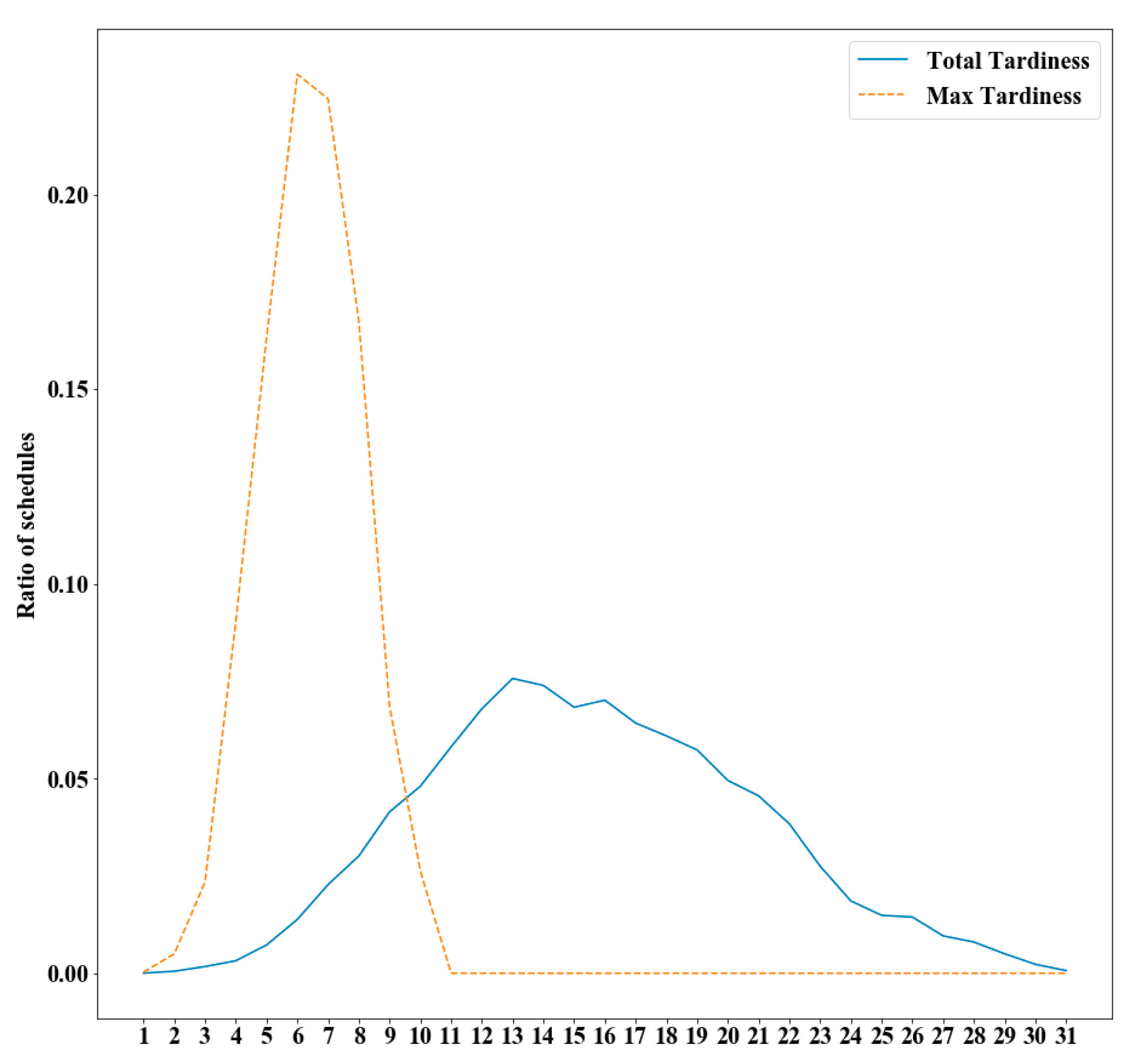
Subsequently, this result was compared with that obtained by the exhaustive search. All possible schedules were generated by considering the processing order of batches as well as grouping jobs. This results in a total of 1,300,561,920 schedules. Each schedule’s total tardiness and maximum tardiness were calculated, and Figure 5 plots the distributions of them for all schedules.
There are 55,296 schedules (0.0042% among all the possible schedules) with a total tardiness of 1, and it is confirmed that the schedule obtained from the trained neural network is included in the 55,296 schedules.
We performed an additional experiment with problem sizes similar to those mentioned above to obtain the schedule with the minimum total tardiness via the proposed approach and then compare them with the optimal schedule. We randomly generated 1000 datasets that included 2, 3, and 4 machines with capacities of 3, 4, 5, and 6, and the numbers of jobs were 8, 9, 10, 11, 12, 13, 14, and 15. In the experiment, job characteristics were randomly generated based on Table 4. The results indicate that the proposed approach obtains the optimal schedules in 948 datasets out of 1000 datasets. Based on the result, we conclude that the proposed approach can establish the optimal schedule for small problems in most cases.
5.3. Comparison with Single Dispatching Rule
In this subsection, we compare the proposed framework with cases of single dispatching rule when there are hundreds of jobs, thereby resulting in a computationally intractable optimal batch schedule. The experiment involves demonstrating that the proposed method can be applied to a real-sized problem and exhibits an excellent performance.
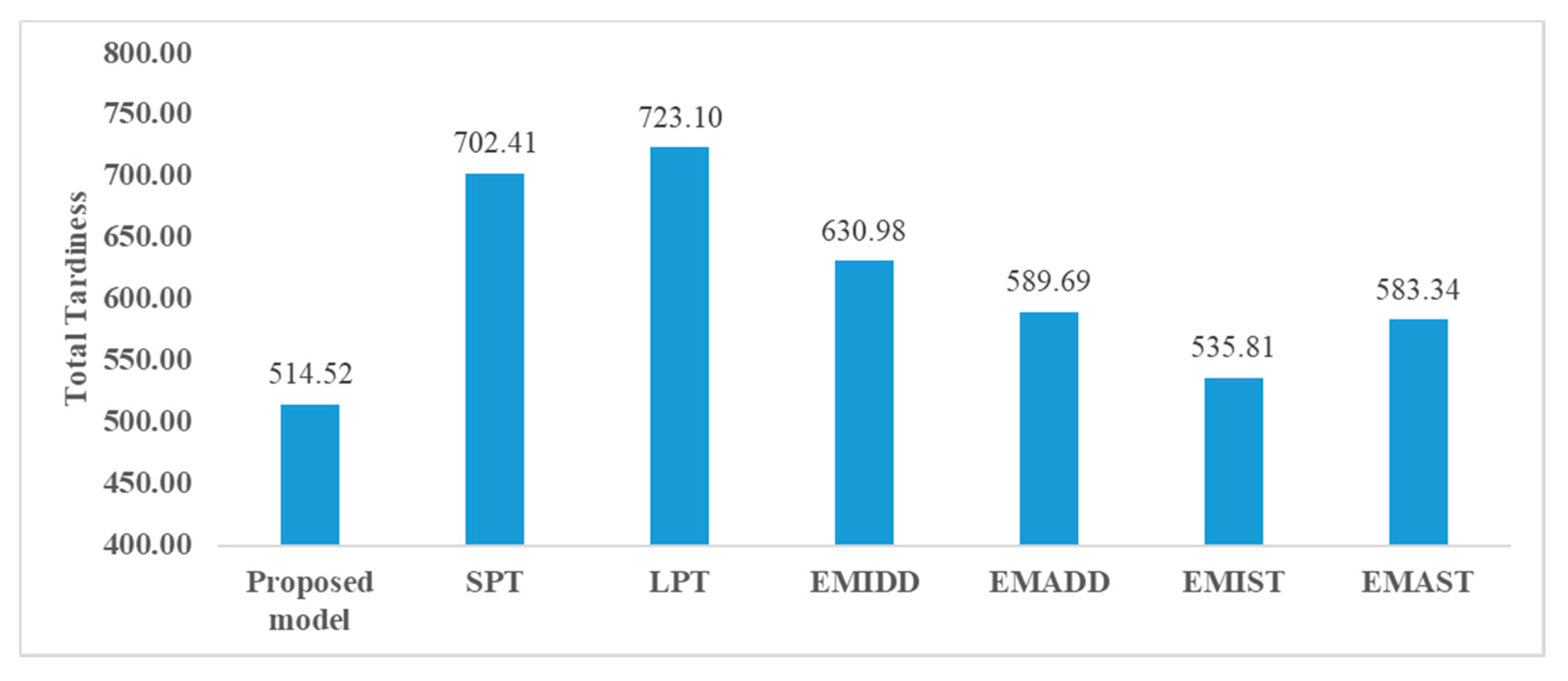
We generated 100 test datasets via Table 4 and Table 5 where each dataset contained 300 jobs and there were four identical machines wherein all the capacities were 6. Subsequently, we applied the clustering algorithm to each dataset. The dispatching rule selection model was then applied to the batches, and the average total tardiness was calculated. This was compared with the cases wherein single dispatching rules (Shortest processing time first (SPT), Longest processing time first (LPT), Earliest minimum due date first (EMIDD), Earliest maximum due date first (EMADD), Earliest minimum release time first (EMIST), and Earliest maximum release time first (EMAST)) were adopted to the same datasets. Figure 6 shows the average total tardiness over all the datasets.
As shown in Figure 6, the proposed model yields the least average total tardiness among all dispatching rules, and this is approximately 4–40% less than the other models. Therefore, it is concluded that the proposed dispatching model yields a more efficient schedule when compared to that of the single dispatching rule, even with respect to a real-sized batch scheduling problem. The proposed model shows only a slight improvement compared to EMIST. This is because this rule seems to be appropriate for the test datasets and the proposed model selects the most appropriate dispatching rule among the pre-defined rules (i.e., SPT, LPT, EMIDD, EMADD, EMIST, and EMAST). It implies that the proposed model relies on the pre-defined rules, and therefore, it is important to consider various rules as pre-defined rules for practical usage.
6. Conclusions
The batch scheduling problem is one of the most important scheduling problems in the manufacturing process, and consists of two subproblems: grouping jobs into batches and determining the sequence of batches. Heuristic approach is a typical way to solve these problems because they are NP-hard (Non-deterministic Polynomial-time hard). However, the heuristic algorithm has the evident limitation that it needs to be designed differently according to the specific problem. In addition, much previous research has addressed only one of those two subproblems.
Motivated by these issues, in this study, we developed a batch scheduling model that is not problem specific and can solve both subproblems. The model consists of a clustering model and dispatching rule selection model to solve the problems of grouping jobs and sequencing batches during batch scheduling, respectively. The clustering model is developed based on the constrained k-means algorithm using a set of features impacting total tardiness (e.g., due date, processing time, and arrival time) and yields clusters that contain jobs wherein the sums of job sizes do not exceed the machine load capacity. The dispatching rule selection model is a supervised model that uses queue state variables (e.g., the number of batches in the queue and maximum processing time of the batches) as features and the most appropriate dispatching rule as the class label. The results of the experiment indicated that the framework solves batch scheduling problems and yields a good batch schedule.
With respect to future work, the proposed framework can be extended to solve diverse batch scheduling problems, for example, modification of the clustering algorithm to include machine capacities that are not identical wherein different types of objective functions are introduced. Additionally, more queue state variables (which cover various batch scheduling problems) can be adopted to make problems more practical.
Author Contributions
Funding acquisition, S.H.; Investigation, G.A.; Methodology, G.A. and S.H.; Software, G.A.; Validation, G.A.; Writing—original draft, G.A.; Review and editing, S.H. All authors have read and agreed to the published version of the manuscript.
Funding
This work was supported by the National Research Foundation of Korea (NRF) grant funded by the Korea government (MSIT) (2019R1A2C1088255).
Conflicts of Interest
The authors declare no conflict of interest.
References
- Vanchipura, R.; Sridharan, R.; Babu, A.S. Improvement of constructive heuristics using variable neighbourhood descent for scheduling a flow shop with sequence dependent setup time. J. Manuf. Syst. 2014, 33, 65–75. [Google Scholar] [CrossRef]
- Ahn, G.; Park, M.; Park, Y.J.; Hur, S. Interactive Q-Learning Approach for Pick-and-Place Optimization of the Die Attach Process in the Semiconductor Industry. Math. Probl. Eng. 2019, 2019, 4602052. [Google Scholar] [CrossRef]
- Mouelhi-Chibani, W.; Pierreval, H. Training a neural network to select dispatching rules in real time. Comput. Ind. Eng. 2010, 58, 249–256. [Google Scholar] [CrossRef]
- Shiue, Y.R. Data-mining-based dynamic dispatching rule selection mechanism for shop floor control systems using a support vector machine approach. Int. J. Prod. Res. 2009, 47, 3669–3690. [Google Scholar] [CrossRef]
- Mönch, L.; Zimmermann, J.; Otto, P. Machine learning techniques for scheduling jobs with incompatible families and unequal ready times on parallel batch machines. Eng. Appl. Artif. Intell. 2006, 19, 235–245. [Google Scholar] [CrossRef]
- Xu, R.; Chen, H.; Li, X. A bi-objective scheduling problem on batch machines via a Pareto-based ant colony system. Int. J. Prod. Econ. 2013, 145, 371–386. [Google Scholar] [CrossRef]
- Damodaran, P.; Srihari, K. Mixed integer formulation to minimize makespan in a flow shop with batch processing machines. Math. Comput. Model. 2004, 40, 1465–1472. [Google Scholar] [CrossRef]
- Shiue, Y.R.; Guh, R.S.; Tseng, T.Y. Study on shop floor control system in semiconductor fabrication by self-organizing map-based intelligent multi-controller. Comput. Ind. Eng. 2012, 62, 1119–1129. [Google Scholar] [CrossRef]
- Tsai, C.F. Feature selection in bankruptcy prediction. Knowl. Based Syst. 2009, 22, 120–127. [Google Scholar] [CrossRef]
- El-Bouri, A.; Shah, P. A neural network for dispatching rule selection in a job shop. Int. J. Adv. Manuf. Technol. 2006, 31, 342–349. [Google Scholar] [CrossRef]
- Chen, H.; Du, B.; Huang, G.Q. Scheduling a batch processing machine with non-identical job sizes: A clustering perspective. Int. J. Prod. Res. 2011, 49, 5755–5778. [Google Scholar] [CrossRef]
- Rodger, J.A. An expert system gap analysis and empirical triangulation of individual differences, interventions, and information technology applications in alertness of railroad workers. Expert. Syst. Appl. 2020, 144, 113081. [Google Scholar] [CrossRef]
- Bilyk, A.; Mönch, L.; Almeder, C. Scheduling jobs with ready times and precedence constraints on parallel batch machines using metaheuristics. Comput. Ind. Eng. 2014, 78, 175–185. [Google Scholar] [CrossRef]
Figure 1.
Batch scheduling problem.

Figure 2.
Step-by-step process.

Figure 3.
Structure of samples of batches in the queue dataset.

Figure 4.
Clustering algorithm example.

Figure 5.
Total and max tardiness distribution.

Figure 6.
Comparison results of the proposed model and single dispatching rule.


Table 1.
Queue state variables.
| Variable | Description |
|---|---|
| Number of batches in the queue. | |
| , , , | Maximum, minimum, average, and standard deviation of the number of jobs in batches in the queue, respectively. |
| , , , | Maximum, minimum, average, and standard deviation of the processing time of batches in the queue, respectively. |
| , , , | Maximum, minimum, average, and standard deviation of the slack time at current time of jobs in the queue, respectively. |
| , , , | Maximum, minimum, average, and standard deviation of the time remaining before the due date of the jobs, respectively. |
| , , , | Maximum, minimum, average, and standard deviation of waiting times of the jobs, respectively. |
Table 2.
Considered candidate dispatching rules.
| Dispatching Rule | Batch with the Highest Priority |
|---|---|
| Shortest processing time first (SPT) | |
| Longest processing time first (LPT) | |
| Earliest minimum due date first (EMIDD) | |
| Earliest maximum due date first (EMADD) | |
| Earliest minimum release time first (EMIRT) | |
| Earliest maximum release time first (EMART) | |
| Earliest minimum slack time first (EMIST) | |
| Earliest maximum slack time first (EMAST) |
Table 3.
Structure of the training dataset for the dispatching rule selection model.
| Time | Optimal Rule | |||||
|---|---|---|---|---|---|---|
Table 4.
Pmfs (probability mass functions) of the job characteristics.
| 1 | 0.30 | 0.30 | 0.25 |
| 2 | 0.40 | 0.40 | 0.25 |
| 3 | 0.30 | 0.30 | 0.25 |
| 4 | 0.00 | 0.00 | 0.25 |
Table 5.
Cpmfs (conditional probability mass functions) of job characteristics.
| (a) Processing Time | (b) Slack Time | |||||||
|---|---|---|---|---|---|---|---|---|
| 1 | 2 | 3 | 1 | 2 | 3 | 4 | ||
| 0.924 | 0.076 | 0.001 | 0.836 | 0.146 | 0.019 | 0.000 | ||
| 0.048 | 0.902 | 0.050 | 0.153 | 0.728 | 0.097 | 0.022 | ||
| 0.001 | 0.071 | 0.928 | 0.014 | 0.098 | 0.815 | 0.073 | ||
| 0.003 | 0.009 | 0.075 | 0.913 | |||||
Table 6.
Job characteristics.
| 1 | 1 | 2 | 2 |
| 2 | 3 | 1 | 5 |
| 3 | 3 | 2 | 4 |
| 4 | 1 | 2 | 3 |
| 5 | 3 | 3 | 6 |
| 6 | 2 | 1 | 4 |
| 7 | 3 | 2 | 5 |
| 8 | 3 | 2 | 4 |
| 9 | 2 | 1 | 2 |
| 10 | 3 | 3 | 6 |
© 2020 by the authors. Licensee MDPI, Basel, Switzerland. This article is an open access article distributed under the terms and conditions of the Creative Commons Attribution (CC BY) license (http://creativecommons.org/licenses/by/4.0/).
Share and Cite
MDPI and ACS Style
Ahn, G.; Hur, S. Clustering and Dispatching Rule Selection Framework for Batch Scheduling. Mathematics 2020, 8, 80. https://0-doi-org.brum.beds.ac.uk/10.3390/math8010080
AMA Style
Ahn G, Hur S. Clustering and Dispatching Rule Selection Framework for Batch Scheduling. Mathematics. 2020; 8(1):80. https://0-doi-org.brum.beds.ac.uk/10.3390/math8010080
Chicago/Turabian StyleAhn, Gilseung, and Sun Hur. 2020. "Clustering and Dispatching Rule Selection Framework for Batch Scheduling" Mathematics 8, no. 1: 80. https://0-doi-org.brum.beds.ac.uk/10.3390/math8010080
Note that from the first issue of 2016, this journal uses article numbers instead of page numbers. See further details here.