Mathematical Model and Evaluation Function for Conflict-Free Warranted Makespan Minimization of Mixed Blocking Constraint Job-Shop Problems

Abstract

In this paper, we consider a job-shop scheduling problem with mixed blocking constraints. Contrary to most previous studies, where no blocking or only one type of blocking constraint was used among successive operations, we assume that, generally, we may address several different blocking constraints in the same scheduling problem depending on the intermediate storage among machines, the characteristics of the machines, the technical constraints, and even the jobs. Our objective was to schedule a set of jobs to minimize the makespan. Thus, we propose, for the first time, a mathematical model of the job-shop problem taking into account the general case of mixed blocking constraints, and the results were obtained using Mosel Xpress software. Then, after explaining why and how groups of jobs have to be processed, a blocking constraint conflict-free warranted evaluation function is proposed and tested with the particle swarm optimization and genetic algorithm methods. The results prove that we obtained a near-optimal solution to this problem in a very short time.

1. Introduction and Targeted Contribution

Many studies have addressed the classic job-shop (JS) problem since Jackson’s first work on the subject [1]. Scheduling issues are still currently of interest, as well as the methods used to address them, since the need for punctuality and customer satisfaction is paramount in our more connected lives. Dynamic scheduling with simulation models can be a way of tackling the problem, as implemented by Turker et al. [2]. Evolutionary algorithm approaches are well known, very efficient, and still currently being investigated and developed for the job-shop problem [3], as well as for flexible job-shop scheduling problems [4]. Moreover, the technical constraints and technologies applied in production systems generate different types of blocking situations. In this paper, to address problems that are likely to be encountered in real industrial environments, we focus on a particular case where different blocking constraints are mixed in the same JS problem. The contribution of this work is the proposal of a mathematical model and two meta-heuristics based on an evaluation function that we developed to solve a general case of a JS problem which could be simultaneously subjected to different types of blocking constraints.

The target audience for the contributions of this paper is both academics and practitioners. Indeed, we propose a mathematical model which further studies in the field of mixed blocking constraints applied to JS problems will lean on. This model aligns itself with existing job-shop models in the literature; however, in our opinion, this is the first time that a job-shop model has taken into account the general case of mixed blocking constraints. The paper should also be of interest to readers in the areas of scheduling theory, combinatorial optimization, and approximation methods. Furthermore, for practitioners interested in solving everyday JS problems with mixed blocking constraints, in this paper, we provide a methodology for solving this problem with any classical optimization method (see Section 5).

The original aspect of this work is that it focuses on the ability to simultaneously take into account different blocking constraints throughout successive operations of a job in a given problem (as opposed to only one type of blocking constraint throughout all operations). From an experimental point of view, we explain why and then how the groups of jobs must be processed to create a conflict-free (viable) evaluation function. We then design an evaluation function, making it possible to use classic and simple algorithms to solve the problem. Then, from both theoretical and experimental points of view, we use the genetic algorithm and particle swarm optimization algorithm to illustrate the feasibility of the method by performing optimization on problems with five jobs/five machines and ten jobs/five machines. The accuracy of our method is discussed using the problems for which the mathematical model gave solutions in a relatively short amount of time. In the case of the problems for which the mathematical model was not able to obtain results in a sufficiently short time, the method we propose was able to give a feasible solution in a very short time.

The possible industrial applications of the solutions proposed in this paper include but are not limited to machining and adjustments, or tool-dependent machining. For jobs in which successive operations give way to adjustments, the nature of the aimed adjustment and the possible corrective procedure give way to different blocking constraints in a job, as detailed in Section 3. Another case of an industrial application is when a job is dependent on a tool, which “follows” it from one operation to another, depriving the first machine of the tool for the time it is used in the subsequent operation. This situation can occur during stamping operations, for example. Moreover, tools and other required equipment may also be regarded as additional resource requirements. For example, the throughput of a coal export terminal and the delays incurred by ships and trains can be greatly affected by where a material is stacked and reclaimed, and which machinery is used to perform those tasks [5].

Blocking constraints are presented in detail in Section 3, but practical applications of RSb blocking constraints can be seen in the processes of block concrete [6], robotic cells [7], iron and steel industries [8], and electronic manufacturing shops [9], among others. Some uses of the RSb blocking constraint have also been applied to the assignment of individual renewable resources in scheduling [10]. Examples of RCb and RCb∗ constraints can be seen in the fabrication of aeronautic parts and the waste treatment industry, as described in Martinez’s works [11], as well as in cider brewing operations [12]. Railway operations are also an application of the RCb blocking case [13].

This paper is organized as follows: after this introduction, a literature review is given in Section 2. Then, in Section 3, we specifically describe the blocking constraints taken into account in the JS problem. A mathematical model is presented in Section 4, for obtaining optimal solutions to these problems. This model also gives us optimal solutions to evaluate the quality of the approximate methods that we developed for larger problems. In Section 5, we present the evaluation function that we developed to be used in two proposed meta-heuristics: the particle swarm optimization method (PSO) and the genetic algorithm (GA). This evaluation function grants a viable, conflict-free warranted solution to any problem size, using any blocking constraint configuration. In Section 6, we present the computational results and the performance evaluation. The last section concludes the paper and gives some other perspectives on our work.

2. Literature Review

According to the literature related to the classic JS scheduling problem, we note that many researchers have made profound contributions. Two complete and interesting review papers investigated both exact methods and approximate algorithms applied to job shop problems, in which readers can find a complete solutions panel [14,15]. Furthermore, Liu and Kozan presented in 2009 an approach to schedule trains as a blocking parallel-machine JS scheduling problem [16]. Blocking constraints have also been used to schedule different transportation traffic methods, such as aircrafts, metros and trains [17]. A single-track railway scheduling problem with three stations and constant travel times between any two adjacent stations has also been addressed with a two-machines jobshop scheduling problem, with equal processing times on each machine [18]. Salido et al. proposed in 2016 an extension of the classic JS scheduling problem in which machines can work at different speeds, and they developed a genetic algorithm to solve this problem [19]. Another search algorithm was proposed for solving JS scheduling problems [20]. This algorithm is called the waterweeds algorithm, and it imitates the reproduction principle of waterweeds in searching for water sources. In another context, a formulation in the form of a mixed-integer linear program (MILP) was proposed to model the JS scheduling problem with non-anticipatory, per-machine, sequence-dependent setup times. The electromagnetism-like algorithm has also been adapted to solve this problem under the minimization of the makespan constraint [21]. Whale optimization is a new swarm-based algorithm which mimics the hunting behavior of humpback whales in nature. It has also been successfully used to solve jobshop problems [22], as well flexible ones [23], with energy efficiency concerns [22,24]. We took particular interest in the particle swarm optimization method (PSO). This optimization method is very promising, with its simple structure and fast convergence speed [25]. In AitZai and Boudhar’s work [26], the PSO algorithm is proven as a performing method to solve jobshop scheduling problems, in the case where all blocking constraints between the operations are RSb. We developed a PSO algorithm to solve the problems addressed in this paper. Since our stopping criteria was the maximum number of iterations for which the best solution remains unchanged, the convergence speed can be seen in terms of CPU time, as well as in terms of solution quality. Indeed, when the swarm is far from the optimal solution, it is much easier to improve the solution than when it is close to the optimal.

A lot of researchers have applied JS scheduling to material handling. A recent review paper summarizes how these problems are solved in dynamic and static problem settings [27]. In the same context, a mathematical programming approach has been proposed to optimize the material flow in a flexible JS automated manufacturing system, given the demand fluctuations and machine specifications [28]. The no-wait job shop scheduling problem approximability under the makespan criterion has been investigated [29]. It has been shown to be APX-hard for the case of two machines with at most five operations per job, and for the case of three machines with at most three operations per job. In complexity theory, an APX-hard problem is an NP-hard problem, which admits a solution with a polynomial-time approximation algorithm with an approximation ratio bounded by a constant. APX is an abbreviation of “approximable”. Problems of this class admit efficient algorithms that give solutions within some multiplicative factor of the optimal. For a generalization of the job shop problem, which takes into account transfer operations between machines and sequence-dependent setup times as well as the Release when Starting blocking constraint (RSb), a Tabu search and a neighborhood have been developed [30]. The problem has been formulated in a generalized disjunctive graph, and a neighborhood for local search has been developed. In contrast to the classical job shop, there is no easy mechanism for generating feasible neighbor solutions. Two structural properties of the underlying disjunctive graph have been established, as well as the concept of closures and a key result on short cycles. Two iterative improvement algorithms have been proposed [31]: an adaptation of an existing scheduling algorithm based on the Iterative Flattening Search, and an off-the-shelf optimization tool, the IBM ILOG CP Optimizer, which implements Self-Adapting Large Neighborhood Search. The results confirm the effectiveness of the iterative improvement approach in solving these kinds of problems. Both variants perform as well individually as together in improving existing solutions. In the same context, an iterated greedy meta-heuristic to solve a JS scheduling problem with blocking constraints has been proposed, and validated by good performances with respect to other state-of-the-art algorithms [32]. Moreover, the authors of this method wrote it to be conceptually easy to implement, and it has a broad applicability to other constrained scheduling problems. For the Release when Completing blocking (RCb) constraint, a MILP and a meta-heuristic have been presented [33] for the job-shop and hybrid job-shop cases. Nevertheless, to our knowledge, only a few works, such as Martinez’s [11] and Trabelsi et al. [12], address JS optimization with this particular blocking constraint (RCb and RCb* constraints). In Trabelsi et al. work [33], we proposed heuristics and meta-heuristics to address job-shop problems with mixed blocking constraints. For the hybrid job-shop (HJS) problem, a mathematical model and a lower bound have been proposed [33], in which a uniform blocking constraint is taken into account among all the operations. A tabu search method has been performed to solve jobshop problems with RSb blocking constraint between all the operations [34,35]. In Bürgy’s work [36], feasible neighborhoods were generated by extracting a job from a given solution and reinserting it into a neighbor position, and five regular objective functions (makespan, total flow time, total squared flow time, total tardiness, and total weighted tardiness) were considered.

Very recently, a paper has been published about neighborhood structures and repair techniques for RSb blocking jobshop scheduling problems with the Total Tardiness minimization criteria, where the concept of feasibility guarantee is noticeably also addressed [37]. The authors used list index to check and retrieve the feasibility of a blocking jobshop schedule given by a single list of operations, and chose a simulated annealing algorithm to perform their experiments. They address the feasibility problem after the scheduling with what they call the Basic Repair Technique (BRT).

In this paper, we present an evaluation function which guarantees the feasibility before scheduling, for any mixed blocking constraint matrix composed of any of the {Wb, RSb, RCb*, RCb} blocking constraints.

3. Problem Description

In the classic JS scheduling problem, a set of n jobs, J = {J₁, J₂, …, J_n}, must be processed on a set of m machines, M = {M₁, M₂, …, M_m}. Each job J_i is composed of n_i operations O_ij = {O_i1, O_i2, …, O_ini} that must be processed on only one machine M_ij according to the manufacturing process. Each machine cannot execute more than one operation at a time. Operation O_ij needs an execution time P_ij on machine M_ij ∊ M. In this paper, a pre-emptive operation is not authorized, and the objective function is to find the best schedule to reduce the makespan (i.e., the completion time of the last operation).

In the following, we present the classic JS without blocking, as well as three different cases of blocking situations in such a problem. To illustrate the difference among these blocking situations, we consider the same example of a JS with four jobs and three machines, and we present its Gantt chart in Figure 1. The routing of each of the four jobs is as follows: J₁ is processed on M₁ and M₃, J₂ is processed on M₂, M₁ and M₃, job J₃ is processed only on M₃, and J₄ is processed on M₂, M₁, and M₃.

For the classic JS case where there is no blocking constraint (Wb), the storage capacity is considered unlimited. Then, a machine is immediately available to process its next operation, after its operation that is in progress is finished (Figure 1a). In industrial applications, when no particular adjustment is needed in the next machines after an operation, we are in the case of a Wb constraint.

In the Release when Starting blocking (RSb) case, we consider that there is no place in stock. Thus, a job remains blocked on a machine as long as the following machine that is in process is not available. We can see an example in Figure 1b where the job J₂ remains blocked on the machine M₁ as long as its next operation starts processing on the machine M₃. In industrial applications, this blocking constraint is encountered when a job adjustment is needed on the next machine.

For this particular Release when Completing blocking (RCb*) case, a machine is released of its job when the following operation on the next machine that is in process is finished. As shown in the example presented in Figure 1c, the machine M₂ remains blocked by job J₂ until its operation on machine M₁ is finished. In industrial applications, such a blocking constraint is encountered when the work done on the first machine still blocks this machine during the period it is operated on the next one. This blocking constraint occurs for example in the cider industry. Let us consider that the vat filling is the first machine, and the second machine is the runway which takes the apples in the vat to bring them to the press. When you want to make the cider only with a given variety of apples, you need to wait for the complete emptying of the first apple variety before filling the vat again with new apples. This is a practical illustration of the application of the RCb* constraint.

As seen in the example presented in Figure 1d, the Release when Completing blocking (RCb) case differs from the RCb* constraint in the fact that it is not sufficient for the job J₂ to have finished its operation on machine M₁, but it should leave it for the next one (M₃) to release machine M₂. Therefore, this blocking constraint links together three machines around the same job. In industrial applications, such a blocking constraint is encountered when the operations made on the first and second machines must allow the job to be mounted in the third machine. This constraint is also used for train scheduling [16].

In this paper, we study a JS problem with mixed blocking constraints. To describe this kind of problem, we introduce a matrix A that contains blocking constraints among operations. Thus, A_ij is the blocking constraint between operations O_ij and O_ij+1. A is then an n by m–1 matrix (n rows and m–1 columns). We attribute different values to blocking constraints to identify them correctly in computing programs. Value 0 is attributed either to the Wb constraint, or when the job has no more operation to be executed. When the job has no more operations to execute (see J₃ on Figure 2), 1 is attributed to the RSb, 2 is attributed to the RCb* constraint, and 3 is attributed to the RCb constraint. The following matrix A is considered and applied to the previous example. The related Gantt chart is then obtained (Figure 2):

4. Mathematical Model

Job-shop problems have been known to be NP-hard for a long time. However, mathematical model development remains a key issue to evaluate the methods that we develop. In this paragraph, we present the extension of the JS mathematical model [38] to the mixed blocking constraint problem, with the makespan as an objective function. First, an extension of the basic JS model was implemented that only takes into account the RCb constraint [5]. Here, the modifications for the possibility to choose any blocking constraint (Wb, RSb, RCb* or RCb) between any two operations is taken into account with the Bk_ij parameters. These parameters are used in Equations (3)–(8).

4.1. Parameters

The model parameters are defined as follows:

n: number of jobs.

m: number of machines.

In this model, the number of machines is also the maximal number of operations treated by a job.

n_i: number of operations of job J_i.

O_ij: j^th operation of job J_i.

O_i = {O_i1, O_i2, …, O_ini}: Set of operations to be executed for job J_i.

p_ij: Processing time of operation O_ij.

M_ij: Machine needed to process operation O_ij.

$\lambda ={\displaystyle \sum _{i=1}^n{\displaystyle \sum _{j=1}^{n_i}{P}_{ij}}}$. It is a high value constant.

$L{0}_{ij}=\{\begin{array}{ll}1\hfill & \mathit{if}j\le ni-2\hfill \\ 0\hfill & else\hfill \end{array}$, ⬄ O_ij is neither the last nor the penultimate operation of job J_i.

$L{1}_{ij}=\{\begin{array}{ll}1\hfill & \mathit{if}j=ni-1\hfill \\ 0\hfill & else\hfill \end{array}$, ⬄ O_ij is the penultimate operation of job J_i.

$L{2}_{ij}=\{\begin{array}{ll}1\hfill & \mathit{if}j=ni\hfill \\ 0\hfill & else\hfill \end{array}$, ⬄ O_ij is the last operation of job J_i.

$\begin{array}{l}B{k}_{ij}=\{\begin{array}{ll}1\hfill & \mathit{if}\mathit{after}{O}_{ij}\mathit{blocking}\mathit{constraint}k\mathit{is}\mathit{valid}\hfill \\ 0\hfill & \mathit{else}\hfill \end{array},\\ \hspace{1em}\hspace{1em}\mathit{with}\mathrm{k}=0(WB), 1(RSb),2(RCb*),3(RCb)\end{array}$

The decision variables are defined as follows:

Y_i,j,i1,j1 is equal to 1 if operation O_ij precedes operation O_i1j1 on the same machine, and 0 otherwise. Consequently, Y_i,j,i1,j1 and Y_i1,j1,i,j are only defined if operations O_ij and O_i1j1 are operated on the same machine.

S_i,j: Starting time of operation O_ij.

C_max: Makespan or maximal completion time of the scheduling problem.

The mathematical model is defined as follows:

$\min C_{max}$, subject to the following constraints:

$$S_{ij}\ge S_{i(j-1)}+P_{i(j-1)},\forall i\in \left[1,\dots ,n\right],\forall j\in \left[1,\dots ,n_i\right]$$

(1)

$$C_{max}\ge S_{i{n}_i}+P_{i{n}_i},\forall i\in \left[1,\dots ,n\right]$$

(2)

$$S_{ij}\ge 0,\forall i\in \left[1,\dots ,n\right],\forall j\in \left[1,\dots ,n_i\right]$$

(3)

$$Y_{ij{i}_1{j}_1}\in \left\{0,1\right\},\forall i,i_1\in [1,\dots ,n],\forall j,j_1\in [1,\dots ,n_i]/M_{ij}=M_{i_1{j}_1}$$

(4)

$$\begin{array}{c}\begin{array}{cc}{S}_{ij}\ge & [S_{i_1(j_1+2)}·L{0}_{i_1{j}_1}+(S_{i_1(j_1+1)}+P_{i_1(j_1+1)})·L{1}_{i_1{j}_1}\hfill \\ & +(S_{i_1{j}_1}+P_{i_1{j}_1})·L{2}_{i_1{j}_1}-\lambda ·Y_{ij{i}_1{j}_1}]·B{3}_{i_1{j}_1}\hfill \\ & +[(S_{i_1(j_1+1)}+P_{i_1(j_1+1)})·(L{1}_{i_1{j}_1}+L{0}_{i_1{j}_1})\hfill \\ & +(S_{i_1{j}_1}+P_{i_1{j}_1})·L{2}_{i_1{j}_1}-\lambda ·Y_{ij{i}_1{j}_1}]·B{2}_{i_1{j}_1}\hfill \\ & +[S_{i_1(j_1+1)}·(L{1}_{i_1{j}_1}+L{0}_{i_1{j}_1})\hfill \\ & +(S_{i_1{j}_1}+P_{i_1{j}_1})·L{2}_{i_1{j}_1}-\lambda ·Y_{ij{i}_1{j}_1}]·B{1}_{i_1{j}_1}\hfill \\ & +[S_{i_1{j}_1}+P_{i_1{j}_1}-\lambda ·Y_{ij{i}_1{j}_1}]·B{0}_{i_1{j}_1},\hfill \end{array}\\ \forall i,i_1\in \left[1,\dots ,n\right],\forall j\in \left[1,\dots n_i\right],\forall j_1\in \left[1,\dots ,n_{i_1}-2\right]\end{array}$$

(5)

$$\begin{array}{l}\begin{array}{c}\begin{array}{cc}{S}_{i_1{j}_1}\ge & [S_{i(j+2)}·L{0}_{ij}+(S_{i(j+1)}+P_{i(j+1)})·L{1}_{ij}\hfill \\ & +(S_{ij}+P_{ij})·L{2}_{ij}-\lambda ·(1-Y_{ij{i}_1{j}_1})]·B{3}_{ij}\hfill \\ & +[(S_{i(j+1)}+P_{i(j+1)})·(L{1}_{ij}+L{0}_{ij})\hfill \\ & +(S_{ij}+P_{ij})·L{2}_{ij}-\lambda ·(1-Y_{ij{i}_1{j}_1})]·B{2}_{ij}\hfill \\ & +[S_{i(j+1)}·(L{1}_{ij}+L{0}_{ij})\hfill \\ & +(S_{ij}+P_{ij})·L{2}_{ij}-\lambda ·(1-Y_{ij{i}_1{j}_1})]·B{1}_{ij}\hfill \\ & +[S_{ij}+P_{ij}-\lambda ·(1-Y_{ij{i}_1{j}_1})]·B{0}_{ij},\hfill \end{array}\\ \forall i,i_1\in \left[1,\dots ,n\right],\forall j\in \left[1,\dots n_i-2\right],\forall j_1\in \left[1,\dots ,n_{i_1}\right]\end{array}\end{array}$$

(6)

$$\begin{array}{c}\begin{array}{cc}{S}_{ij}\ge & [(S_{i_1(j_1+1)}+P_{i_1(j_1+1)})·L{1}_{i_1{j}_1}\hfill \\ & +(S_{i_1{j}_1}+P_{i_1{j}_1})·L{2}_{i_1{j}_1}-\lambda ·Y_{ij{i}_1{j}_1}]·B{3}_{i_1{j}_1}\hfill \\ & +[(S_{i_1(j_1+1)}+P_{i_1(j_1+1)})·L{1}_{i_1{j}_1}\hfill \\ & +(S_{i_1{j}_1}+P_{i_1{j}_1})·L{2}_{i_1{j}_1}-\lambda ·Y_{ij{i}_1{j}_1}]·B{2}_{i_1{j}_1}\hfill \\ & +[(S_{i_1(j_1+1)}·L{1}_{i_1{j}_1}\hfill \\ & +(S_{i_1{j}_1}+P_{i_1{j}_1})·L{2}_{i_1{j}_1}-\lambda ·Y_{ij{i}_1{j}_1}]·B{1}_{i_1{j}_1}\hfill \\ & +[(S_{i_1{j}_1}+P_{i_1{j}_1})-\lambda ·Y_{ij{i}_1{j}_1}]·B{0}_{i_1{j}_1},\hfill \end{array}\\ \forall i,i_1\in \left[1,\dots ,n\right],\forall j\in \left[1,\dots n_i\right],\forall j_1\in \left[1,\dots ,n_{i_1}-1\right]\end{array}$$

(7)

$$\begin{array}{c}\begin{array}{cc}{S}_{i_1{j}_1}\ge & [(S_{i(j+1)}+P_{i(j+1)})·L{1}_{ij}\hfill \\ & +(S_{ij}+P_{ij})·L{2}_{ij}-\lambda ·(1-Y_{ij{i}_1{j}_1})]·B{3}_{ij}\hfill \\ & +[(S_{i(j+1)}+P_{i(j+1)})·L{1}_{ij}\hfill \\ & +(S_{ij}+P_{ij})·L{2}_{ij}-\lambda ·(1-Y_{ij{i}_1{j}_1})]·B{2}_{ij}\hfill \\ & +[(S_{i(j+1)}·L{1}_{ij}\hfill \\ & +(S_{ij}+P_{ij})·L{2}_{ij}-\lambda ·(1-Y_{ij{i}_1{j}_1})]·B{1}_{ij}\hfill \\ & +[(S_{ij}+P_{ij})-\lambda ·(1-Y_{ij{i}_1{j}_1})]·B{0}_{ij},\hfill \end{array}\\ \forall i,i\in \left[1,\dots ,n\right],\forall j\in \left[1,\dots n_i-1\right],\forall j_1\in \left[1,\dots ,n_{i_1}\right]\end{array}$$

(8)

$$\begin{array}{ll}{S}_{ij}\ge & [(S_{i_1{j}_1}+P_{i_1{j}_1})·L{2}_{i_1{j}_1}-\lambda ·Y_{ij{i}_1{j}_1}]\hfill \\ & \forall i,i_1\in \left[1,\dots ,n\right],\forall j\in \left[1,\dots n_i\right],\forall j_1\in \left[1,\dots ,n_{i_1}\right]\hfill \end{array}$$

(9)

$$\begin{array}{ll}{S}_{i_1{j}_1}\ge & [(S_{ij}+P_{ij})·L{2}_{ij}-\lambda ·(1-Y_{ij{i}_1{j}_1})]\hfill \\ & \forall i,i_1\in \left[1,\dots ,n\right],\forall j\in \left[1,\dots n_i\right],\forall j_1\in \left[1,\dots ,n_{i_1}\right]\hfill \end{array}$$

(10)

The modelled constraints are, on the one hand, the precedence constraints of the successive operations of a given job (1), and on the other hand the precedence constraints of the operations processed on a given machine of a given stage. Equation (2) defines C_max as the latest completion time of an operation. Equation (3) and Equation (4) define that all starting times are positive and that Y_iji1j1 is binary, respectively. The Y variable is used in this model to choose the correct blocking constraints in the inequalities (5)–(10), when they need to be taken into account. For each couple of operations following each other on the same machine, since we do not know which operation will be scheduled before the other, two equations have to be written to model this precedence constraint (Equations (5)–(10)). For example, let us take Equations (5) and (6). If O_ij precedes O_i1j1, then Equation (5) is always verified with λ variable (big M), and we consider Equation (6). If not, we are in the inverse case, Equation (6) is always verified, and we only consider Equation (5). This is the classical disjunctive constraint expression. In what follows, we explain what happens if operation O_i1j1 directly follows operation O_ij, with Equation (6). Then, first we have Y_iji1j1 = 1, and thus λ(1 − Y_iji1j1) = 0, which nullifies the big M constraint in this particular case.

If no blocking constraint exists after operation O_ij on job j, independently on operation O_i1j1, then B0_ij = 1, B1_ij = 0, B2_ij = 0 and B3_ij = 0. Equation (6) then simplifies itself as S_i1j1 ≥ S_ij + P_ij, which is the definition of a precedence constraint without blocking.

If an RSb blocking constraint exists after operation O_ij on job j, then B0_ij = 0, B1_ij = 1, B2_ij = 0 and B3_ij = 0. Equation (6) then simplifies itself as S_i1j1 ≥ (S_i(j+1)). (L1_ij + L0_ij) + (S_ij + P_ij). L2_ij. If O_ij is the ultimate operation of job j, then L2_ij = 1 and L1_ij + L0_ij = 0, and Equation (6) becomes S_i1j1 ≥ (S_ij + P_ij) and expresses only a precedence constraint for O_i1j1. However, if O_ij is not the ultimate operation of job j, then L2_ij = 0 and L1_ij + L0_ij = 1, because this operation is either the penultimate, or any other one. In this case, the precedence constraint (6) then becomes S_i1j1 ≥ (S_i(j+1)), which is the expression of the RSb blocking constraint.

If an RCb* blocking constraint exists after operation O_ij on job j, then B0_ij = 0, B1_ij = 0, B2_ij = 1 and B3_ij = 0. Equation (6) then simplifies itself as S_i1j1 ≥ (S_i(j+1) + P_i(j+1)). (L1_ij + L0_ij) + (S_ij + P_ij). L2_ij. The same reasoning as for the RSb constraint applies. Then, if O_ij is the ultimate operation of job j, Equation (6) becomes S_i1j1 ≥ (S_ij + P_ij), and if not it becomes S_i1j1 ≥ (S_i(j+1) + P_i(j+1)), which is exactly the expression of the RCb* blocking constraint.

To conclude, if an RCb blocking constraint exists after operation O_ij on job j, then B0_ij = 0, B1_ij = 0, B2_ij = 0 and B3_ij = 1. Equation (6) then simplifies itself as S_i1j1 ≥ S_i(j+2). L0_ij + (S_i(j+1) + P_i(j+1)). L1_ij + (S_ij + P_ij). L2_ij. If O_ij is the ultimate operation of job j, then L2_ij = 1, L1_ij = 0, and L0_ij = 0, Equation (6) then simplifies itself as S_i1j1 ≥ (S_ij + P_ij) and the constraint becomes only a simple precedence constraint. If O_ij is the penultimate operation of job j, then L2_ij = 0, L1_ij = 1, and L0_ij = 0, and Equation (6) then simplifies itself as S_i1j1 ≥ (S_i(j+1) + P_i(j+1)) and the constraint becomes equivalent to a RCb* blocking constraint. If O_ij is neither the ultimate nor the penultimate operation of job j, then L2_ij = 0, L1_ij = 0, and L0_ij = 1, and Equation (6) then simplifies itself as S_i1j1 ≥ S_i(j+2), which is the expression of the RCb blocking constraint.

Moreover, since the blocking constraints are not expressed in the same way for the penultimate and the last operations of a job, we have to rewrite both respective equations twice. Equations (7) and (8) model the precedence constraints on a machine when an operation is the penultimate operation of its job, and Equations (9) and (10) model the precedence constraints when an operation is the last operation of its job, with the opportune simplifications of Equations (5) and (6).

4.2. Results Obtained on Mixed Blocking Constrained Jobshop Problems

To facilitate new heuristic developments, we decided to adapt some instances of Lawrence [39]. For each sized problem, we arbitrarily generated four blocking matrices, which constitute different situations of mixed blocking constraints. The four matrices used for the 5x5 problem are given in Figure 3. The blocking constraints were duplicated for higher range problems.

The results, which are presented in

Table 1. Mean computation time (in seconds) of the mathematical model with different blocking constraints.

Jobs	Machines	Blocking Constraints
		A1	A2	A3	A4
5	5	0.04	0.03	0.02	0.04
10	5	67.77	33.78	47.44	40.37
10	10	1174.30	618.32	605.60	84.9
15	5	>1 h	>1 h	>1 h	>1 h

, were obtained using the above presented mathematical model, which was computed with Mosel-Xpress software on a 3 GHz/1Go PC.

The mathematical model’s computation time strongly increases with respect to the number of jobs that are treated and the number of machines. As a consequence, to be able to treat it within a reasonable computational time, for each sized problem, in the next section, we propose an evaluation function that is able to adapt any classic meta-heuristic to a JS problem with mixed blocking constraints.

5. Evaluation Function for Meta-Heuristics

Smart solution-finding methods encoded in meta-heuristics allow investigation into wide solution spaces with few evaluated solutions and good accuracy with respect to the computational time spent. Moreover, for some industrial applications, if an exact solution is unavailable, which could be the case if we look at the Table 1 results, a meta-heuristic with the appropriate evaluation function will be more likely to provide a feasible solution. Moreover, another interest of meta-heuristics lies in their ability to produce a good solution in an adjustable amount of time. These methods are well-known and have existed for a long time, and their programming, once done, does not require more effort than developing an adapted evaluation function. This is the reason we propose to design and develop an evaluation function that is able to give feasible solutions and that is blocking constraint conflict-free to be able to tackle harder problems, which makes it more likely to be applicable to industrial range scheduling problems.

For many of these problems, meta-heuristics give solutions close to the optimum in an adjustable time. Meta-heuristics are created for hard optimization problems and utilize features present in a wide variety of natural and biological processes. This is the case for both of the meta-heuristics presented in this paper. Genetic algorithms are well known now for their imitation of chromosomal genetic evolution [40]. They use a chromosome to represent a solution. Genetic crossover and mutation operators, both based upon biological processes imitation, are used. Particle swarm optimization has been introduced more recently [41], and also computationally reproduces the behavior of a group. Here, each individuate evolves in the solution space, starting from a given position and speed. Then, the evolution of each individual is moderated both by the best solution found by the group at the precedent iteration, and by the best solution obtained since the beginning of the run. In both cases, the meta-heuristics attempt to mimic natural processes in a program code to solve a difficult problem.

To solve a problem with a meta-heuristic, it can be sufficient to develop an evaluation function. This function is used to translate problem data into mathematically interpretable solution space data that can be used by the meta-heuristic. With an evaluation function, a meta-heuristic can move solution populations (chromosomes or individuals) into the solution space to represent all the possible solutions and to obtain a minimal value. This minimal value can sometimes be optimal, but there is no means to prove its optimality. In the following section, we describe the way in which we developed an evaluation function adapted to the JS problem with mixed blocking constraint resolution. This evaluation function has been designed to be computed with any meta-heuristic solving method. The complexity of the solving method will mainly depend on the meta-heuristic.

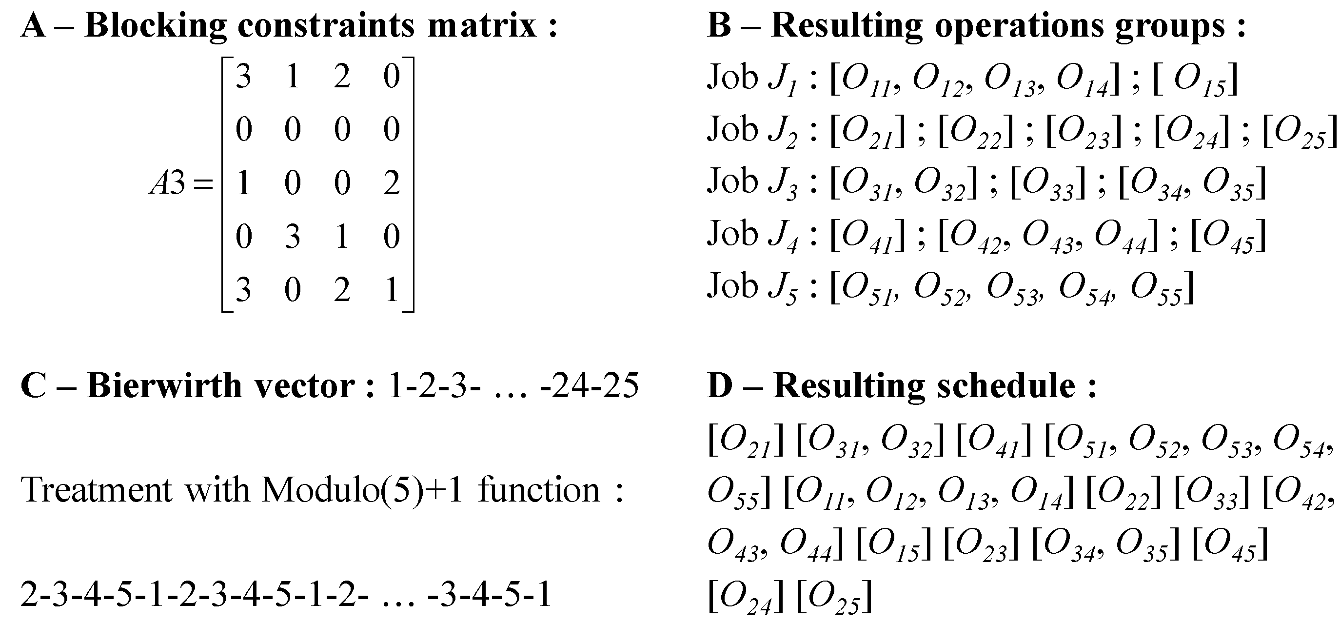
5.1. Bierwirth Vector

In 1995, Bierwirth proposed a vector to adapt JS problems to a resolution with a genetic algorithm [42]. This vector is composed of the job numbers, and each job number is repeated in the vector as many times as its number of operations. These job numbers are ordered in the way that the operations are supposed to be placed on the schedule for the considered sequence. It is sufficient to write a routine that evaluates the objective function with a given Bierwirth vector to find a solution with the meta-heuristic. The activity timings can be determined, for instance, by using a disjunctive graph. This was done in 2010 to construct new train schedules [43]. We chose to use the Bierwirth vector to make our evaluation function generic and usable, not only with the two optimization methods proposed in this paper, but with any other population-based method.

To create our evaluation function, we used chromosomes of n∗m dimensions and with the “modulo(n) + 1” function. Each individual corresponds to a sequence, but a sequence can be described by (m!)n individuals. Nevertheless, to find a solution to the problem, a one-to-one correspondence between chromosomes and sequences is not compulsory. Here, we give an example for a three jobs/four machines problem.

Let us observe the function that attributes a sequence to a given individual. Let us take, for example, the following individual of a classical genetic algorithm: 3-4-1-12-2-8-7-5-9-11-10-6. This individual has, after the “modulo(3) + 1” operation, the following sequence: 1-2-2-1-3-3-2-3-1-3-2-1. This sequence is the Bierwirth sequence corresponding to this individual. This sequence stands for the order in which jobs will be set in the schedule, corresponding to the given individual. Since m operations are considered per job, a given sequence contains m times a job number.

5.2. Evaluation Function

When no blocking constraint exists between operations, a schedule is directly computed from the Bierwirth vector without any additional treatment. Operations are set one after the other in the schedule to calculate the related objective function.

In contrast, in a mixed blocking constraint case, the time at which a machine becomes available depends on the blocking constraints that exist among further job operations. Therefore, determining a feasible schedule is not trivial. We can ensure a conflict-free schedule generation if operations are scheduled coherent set after coherent set. The conflicting situations occurring in job-shop scheduling under blocking constraints have been described and studied thoroughly [33].

A coherent set of operations depends on the successive blocking constraints of a given job. Indeed, to schedule an operation followed by a Wb constraint, we do not need to know how its following operation is scheduled to know when the machine will be released. To schedule an operation followed by either an RSb or an RCb* constraint, we have to know how its following operation is scheduled to free the machine on which it is processed, either to free it at the start or the completion time of the following operation on its next machine. When an RCb constraint follows the in-course operation, we need data not only on the next operation scheduling, but also on further subsequent operation starting times. The implications of the different blocking constraints on the release time of a machine are presented in Figure 4.

Then, to close a coherent set of operations, we have to consider the series of blocking constraints among operations. An RCb constraint directly enforces at least the next two operations to schedule the in-course operation. Similarly, an RCb* and an RSb constraint both enforce one to only consider at least the next operation to schedule an in-course operation. Successively, blocking constraints are taken into account to group together operations. In all cases, a group of operations has to be finished by an operation followed by a Wb constraint to make a coherent set, since this last operation needs no additional data to be scheduled. If not, we continue to take into account the next blocking constraint to add to the group’s further operations. This is the way we go from a blocking constraint matrix to a set of operations, as presented in Figure 5 from step A to step B.

When sets of operations are built, all that remains is to evaluate the Bierwirth vector that is passed as the input data of the evaluation function. To calculate the makespan, for example, we have to set groups of operations in the order given by the Bierwirth vector. Indeed, a job operation is labelled with its job number. Groups of operations are set in the schedule in exactly the same way as the operations in the original use of the Bierwirth vector.

The grouping operations make the last numbers of the Bierwirth vector useless. We chose to keep the totality of the vector because it is possible to consider a case without any blocking constraint, and because there is no need to needlessly complicate the algorithm.

To see how operations are taken into account by the evaluation function, we propose to treat a mixed blocking constraint matrix example with five jobs, each composed of five operations (Figure 5). First, the blocking matrix is translated into groups of operations, job after job. Next, the meta-heuristic vector is translated into a Bierwirth vector using the above-described transformation, modulo (5) + 1, in the presented example. Then, using the function of the resulting Bierwirth vector, groups of operations are put in the schedule in the order of their job number. If all the operations of a job are already placed in a schedule, the evaluation function ignores this number and proceeds to the following one until all operations and groups are placed in the schedule.

5.3. Meta-Heuristics Proposed

The genetic algorithm is a well-known optimization method that was introduced by Holland in 1962, and it has been used in many applications ever since. This method has proved its effectiveness in scheduling problems for a long time [44]. Thus, we chose this meta-heuristic for testing our evaluation function. We developed a genetic algorithm in which we can choose the respective percentages of new individuates introduced into the population, the best people kept from a population to the following step, the crossover, and the mutation. Then, we proposed an improved method based on two representation levels and the definition of meta-genes [45]. We propose to use the genetic algorithm to test the evaluation functional efficiency on the mixed blocking constrained JS problems.

Particle swarm optimization (PSO) is also an evolutionary computation technique that was introduced by Kennedy and Eberhart [41]. The technique of this method was inspired by the behaviors of individuals in a group, such as bird flocking or fish schooling. The PSO approach shares many similarities with genetic algorithms. A comparison between the PSO and GA has been given previously [46]. The PSO algorithm is simple, quick and easy to implement. This method is also attractive because there are few parameters to adjust. PSO has been successfully applied in many research and application areas, such as discrete combinatorial optimization problems. For instance, Xia and Wu demonstrated the application of PSO to a well-known job-shop scheduling problem [47], and Wong and Ngan presented a comparison of the hybrid genetic algorithm and the hybrid particle swarm optimization to minimize the makespan for the assembly job-shop problem [48]. All these arguments motivated us to test our evaluation function in the particle swarm optimization environment as well, both to validate its complete integration and to compare the efficiency of the two methods on this particular problem.

6. Benchmarks and Computing Results

We used the PSO and GA algorithms to perform the experiments. Each method is able to take into account classic individuals that are described with a series of integer values ranging from 1 to the appropriate value with respect to the treated problem. In the genetic algorithm, we can adjust many parameters, such as the population number (nb_indiv), the best individuals kept from the preceding population (pc_best), the new randomly inserted individuals (pc_new), the crossover (pc_cross), and the mutation (completion to 1) percentages. In the particle swarm optimization algorithm, we can tune both the number of particles (nb_indiv) and the acceleration constant (g). In both algorithms, the stopping criterion we chose to implement is the number of times the best solution that is found remained unchanged (ctbvi), because it is a self-adapting stopping criterion, which has given satisfactory outcomes to lots of problems [44]. Indeed, PSO and GA can be used on very different problems, and we cannot know, when developing the method, what the solution space will look like. In order to use the CPU time most effectively, this stopping criterion seems to be the best adapted [45]. Indeed, when the population is relatively far from the optimal solution, it is much easier to improve the solution, and then to re-initialize the counter. On the contrary, when the population comes closer to the optimal, it becomes more difficult. Behind this stopping criterion is the idea that the laptop CPU time will be correctly used most of the time, and only wasted at the very end of the optimization process, when all the ctbvi iterations will be used and the global solution will remain unchanged. In our opinion, a time limit criterion is less problem self-adaptive.

In this section, we give the results obtained on the same four mixed constraint matrices that were used in Section 4. In the particle swarm optimization algorithm, we chose the acceleration constant (g) equal to 1 with the normalized position, speed and acceleration vectors. With respect to the genetic algorithm, we tested different parameters, and those that gave the best results were pc_best = 0.1, pc_new = 0.1, and pc_cross = 0.6. We chose ctbvi = 20 for the stopping criterion. To update the individuates, the crossing step recombines two parents and produces children who inherit some of parental characteristics. Individuals selected for crossing are taken from among the preceding generation’s best individuals and new randomly generated people. The remaining percentage of the created generation is created by mutation. Mutation is a random alteration of an individual’s genes. We selected individuals among the best ones for mutation, to see whether they improved their good results.

The results presented in

Table 2. Average error (in %) of meta-heuristics on mixed blocking constraint job-shop problems.

j	m	Meta-Heuristic	Parameters	A1	A2	A3	A4
5	5	PSO	ctbvi = 10; nb_indiv = 10	22.7	9.6	10.4	21.5
		PSO	ctbvi = 100; nb_indiv = 100	14.8	5.8	5.2	17.0
		GA	ctbvi = 100; nb_indiv = 100	12.6	2.4	2.3	12.3
10	5	PSO	ctbvi = 10; nb_indiv = 10	63.3	59.2	52.4	66.2
		PSO	ctbvi = 100; nb_indiv = 100	49.0	47.6	40.3	51.6
		GA	ctbvi = 100; nb_indiv = 100	40.8	33.3	30.8	22.7

were obtained with our evaluation function, the genetic algorithm, and the PSO algorithm. Each result was obtained in less than 30 s, which means that our evaluation function gives results that could be used in an industrial environment, to obtain results in an adaptable time in the function of the treated problem, with the meta-heuristic’s adaptable settings. For each problem size, the best results are highlighted in bold. We note that the GA performance was better than the PSO in all the tested problems. We can also note that the performance of the PSO algorithm improves its results as ctbvi and nb_indiv increase, but this occurs with a computing time increase, which is not the purpose of this paper. The GA result quality deteriorates rapidly if we observe the difference between the 5j5m and 10j5m problems. This rapid deterioration is due to the conflict-free solution that we warrant with the design of our evaluation function, which is explained later. The results improve from the A1 to the A4 blocking matrices. We can explain this result evolution with a careful observation of these blocking matrices, combined with the design of our evaluation function.

Indeed, when we consider what occurs in the evaluation function between phases A and B, when operations are grouped with respect to the blocking constraints that link them to each other, we can define a “granularity” notion. As presented in Figure 5, the line with job J₂ contains five blocks of one operation when job J₅ contains one block of five operations that are linked together by their successive blocking constraints. The granularity of job J₂ can then be considered as the finest when the one of job J₅ is the largest. Taking into account this notion of granularity, we note that matrices A1 to A4, which are presented in Figure 3, show decreasing granularities. Then, we can easily understand that the results are better for the fine granularity blocking constraint matrix (A4) than for a rough one (A1).

This definition highlights the relatively increasing error in terms of the granularity. Indeed, when we consider the evaluation function design, we can see that it closely depends on the blocking matrix. With a rough granularity matrix that is composed of lines similar to J₅, setting the first operation of a job directly leads to setting all the operations of this job, since they are all linked. However, with a fine granularity matrix that is composed of lines that are mostly similar to J₂, we can set all the operations of a job separately from each other and can input them into the optimization method. Thanks to its problem self-adapting stopping criterion, this method gives a great opportunity to optimize the criterion at each new solution step, which may be either big if we are rather far from the optimal solution, or small if we are closer to the optimal solution.

Our evaluation function is designed and certified to give mixed blocking job-shop schedules without conflicts. Indeed, taking into account the blocking constraints in a JS scheduling problem can lead to conflicts, and can completely ruin the problem resolution [33]. Since we know the possibility of the occurrence of these conflicts, and since we want to give solutions without conflicts, our evaluation function ensures a feasible schedule in a relatively short time that is adjustable due to the optimization method. However, these conflicts could mean that the solutions for which we ensure feasibility are still relatively far from the optimal solution.

Nevertheless, we show the feasibility and validate our method by applying it to the without-blocking case, which has already been widely studied. When we apply to our method to a null blocking matrix, we solve the original Lawrence problems. The solutions that we obtained with both methods are summarized in

Table 3. Results of PSO and GA on Wb job-shop Lawrence benchmarks.

j	m	GA (%)	GA (s)	PSO (%)	PSO (s)
10	5	5.91	0.6	9.47	2.0
10	10	8.24	1.6	12.88	6.6
15	5	1.28	1.2	3.17	4.2
15	10	16.59	3.4	19.90	16.8
15	15	14.56	8.4	18.71	39.2
20	5	0.31	2.4	2.54	6.4
20	10	16.06	8.0	18.91	26.6
30	10	5.60	13.8	9.26	77.2
Average:		8.57		11.86

. The values taken for the GA and PSO algorithm are the same as for previous numerical applications (pc_best = 0.1, pc_new = 0.1, and pc_cross = 0.6, g = 1). For the results presented in Table 3, we chose the same number of individuals or particles for both the GA and PSO algorithms, as nb_indiv = 30, and ctbvi = 20. Since this work is the first regarding mixed blocking constraints and job-shop scheduling, we do not dispose of a set of solutions with a given benchmark. Nevertheless, when we use our method with no blocking constraint, we still found seven and five optimal solutions, out of the 40 Lawrence problems, with these relatively low settings.

To conclude, even if it is not the purpose of this paper, we can briefly compare the results of the GA and PSO. With the results presented in Table 3, we can conclude that the GA outperforms the PSO since its results are more precise and were obtained in a shorter time with the same evaluation function. This brief comparison only shows that, for this mixed blocking constraint job-shop scheduling problem, the two optimization methods that we propose give feasible schedules without conflicts, and the results given by the GA are significantly better in terms of both accuracy and computing time.

This evaluation function has been developed to be able to take into account industrial sized problems. Thus, we have tested its insertion into the genetic algorithm for the Lawrence benchmark instances [39], for problems with up to 100 jobs and 20 machines. The results presented in

Table 4. Results obtained on Lawrence instances with the four blocking patterns presented in Figure 3.

j	m	Blocking Matrix				Execution Time				j	m	Blocking Matrix				Execution Time
		A1	A2	A3	A4	A1	A2	A3	A4			A1	A2	A3	A4	A1	A2	A3	A4
10	5	1512	1167	1217	1127	3	7	3	4	30	10	7792	5101	5295	4421	53	67	63	88
10	5	1503	1140	1172	1086	5	3	4	3	30	10	8204	5742	5289	4836	83	58	79	121
10	5	1278	1050	1086	1004	2	7	2	2	30	10	7814	5126	4949	4819	43	94	161	53
10	5	1212	1025	973	903	4	3	7	4	30	10	7710	5545	4842	4630	49	43	75	150
10	5	1189	945	864	872	3	3	5	3	30	10	7657	4700	5083	4945	48	165	143	82
10	10	2524	1679	1983	1827	8	11	9	6	30	15	8101	6097	5505	5029	102	43	368	306
10	10	2296	1722	1611	1437	6	8	7	9	30	15	7988	5291	5563	4991	68	239	256	384
10	10	2434	1569	1834	1692	19	9	14	6	30	15	7552	5767	5668	4884	198	133	89	179
10	10	2605	1819	1762	1812	15	8	18	6	30	15	8163	5336	5681	4962	87	196	120	193
10	10	2704	1689	1750	1676	6	11	6	17	30	15	8186	5486	5893	4993	80	241	130	307
15	5	2173	1718	1644	1546	8	5	4	4	30	20	8143	6261	5853	5776	302	186	420	243
15	5	1938	1527	1364	1456	12	5	12	10	30	20	8220	6060	6058	5435	139	334	285	399
15	5	2101	1649	1628	1441	10	8	9	11	30	20	7783	5917	6195	5653	302	186	420	243
15	5	2229	1772	1686	1667	7	6	9	11	30	20	8252	6063	6002	5462	338	382	393	251
15	5	1888	1741	1544	1576	12	5	5	10	30	20	7785	6017	6422	5452	292	194	443	275
15	10	3852	2548	2644	2546	19	17	26	18	50	15	12,195	10,046	9615	8598	359	560	523	469
15	10	3592	2431	2232	2487	20	14	18	15	50	15	12,184	9812	9094	8165	230	796	420	390
15	10	3783	2640	2779	2321	25	15	17	11	50	15	11,672	9767	8946	8451	430	613	351	648
15	10	3720	2471	2430	2504	36	14	18	27	50	15	11,977	9512	9712	7647	658	898	414	976
15	10	3749	2572	2358	2310	48	25	29	23	50	15	12,108	9827	8893	8116	545	251	653	832
15	15	5455	3680	3390	3508	31	31	36	29	50	20	13,105	10,386	10,090	9291	556	1935	829	741
15	15	6445	3874	3708	3911	32	32	16	44	50	20	12,582	10,737	9616	8860	754	681	796	981
15	15	5741	3019	3357	3214	61	50	61	42	50	20	12,705	9823	10,344	8852	747	1671	327	1335
15	15	5404	3525	3349	3527	31	22	44	50	50	20	12,579	10,399	9981	9312	902	717	714	981
15	15	5856	3485	3371	3761	21	42	35	47	50	20	13,342	9943	9914	8850	276	1231	1349	1452
20	5	2798	2209	2153	2134	12	15	11	10	100	20	22,632	22,363	20,972	18,108	5547	2517	3130	3251
20	5	2545	1915	1840	1785	8	15	21	15	100	20	23,598	21,479	20,796	17,913	3886	7498	4863	7111
20	5	2725	2235	2211	2115	8	13	15	16	100	20	23,797	20,866	20,584	17,482	3871	5529	2207	6603
20	5	2735	2362	1923	2086	14	11	14	14	100	20	23,925	21,273	20,513	19,538	4709	6505	5209	4375
20	5	2787	2212	2201	2303	12	14	9	13	100	20	24,947	23,354	21,578	19,088	3962	4323	3342	5823
20	10	5405	3507	3777	3462	23	29	17	25
20	10	5139	3610	3453	3294	39	37	39	24
20	10	5175	3451	3276	3599	33	40	47	31
20	10	5185	3477	3150	3176	24	32	29	38
20	10	5375	3907	3324	3564	22	21	27	19

show that our evaluation function is able to obtain adequate results, even with large sized problems. The optimization method struggles more with a larger number of jobs, as well as with a larger number of machines to consider, even if the computation time increase seems to be more sensitive to the number of jobs. Globally, Table 4 proves that we are able to solve industrial problems with this evaluation function, within approximately 20 min for a 50 jobs problem, and within 2 h for a 100 jobs problem.

7. Conclusions and Perspectives

We developed, tested, and validated a mathematical model to solve the JS scheduling problem under mixed blocking constraints among successive operations. Since the mathematical model can become insufficient as a function of the problem size, we also designed, developed, and validated an evaluation function that is able to solve this particular problem with classic meta-heuristics, and we presented the results obtained with this function. Based on its construction, the evaluation function returns blocking constraint conflict-free results. The obtained results of the four mixed blocking problem benchmarks validate the method and allow us to solve a range of problems with a higher number of jobs and machines, in which the accuracy depends on the blocking matrix’s granularity. The notion of the granularity of a blocking matrix was defined in this paper and was illustrated with the computed results. The remaining limits are set by the meta-heuristic self-capacities, and the blocking constraints were not already taken into account in the works that were presented. The compatibility issues with meta-heuristics were treated with the insertion of the evaluation function, with both a genetic algorithm and a particle swarm optimization algorithm.

Future work will further investigate granularity with a more precise definition and evaluation. A supplementary conflict detection procedure could also be interesting to integrate into the evaluation function, but it is still a very difficult method to perform. The adaptation of this method to flexible JS scheduling seems to also be an achievable objective. Another investigation after this work could be the improvement of the meta-heuristic methods. For this, the 2-phase NSGA II algorithm could be an interesting idea [49].

References

1. Jackson, J.R. An extension of Johnson’s result on job lot scheduling. Nav. Res. Logist. Q. 1956, 3, 201–203. [Google Scholar] [CrossRef]
2. Turker, A.; Aktepe, A.; Inal, A.; Ersoz, O.; Das, G.; Birgoren, B. A Decision Support System for Dynamic Job-Shop Scheduling Using Real-Time Data with Simulation. Mathematics 2019, 7, 278. [Google Scholar] [CrossRef] [Green Version]
3. Wu, Z.; Yu, S.; Li, T. A Meta-Model-Based Multi-Objective Evolutionary Approach to Robust Job Shop Scheduling. Mathematics 2019, 7, 529. [Google Scholar] [CrossRef] [Green Version]
4. Sun, L.; Lin, L.; Li, H.; Gen, M. Cooperative Co-Evolution Algorithm with an MRF-Based Decomposition Strategy for Stochastic Flexible Job Shop Scheduling. Mathematics 2019, 7, 318. [Google Scholar] [CrossRef] [Green Version]
5. Burdett, R.L.; Corry, P.; Yarlagadda, P.K.D.V.; Eustace, C.; Smith, S. A flexible job shop scheduling approach with operators for coal export terminals. Comput. Oper. Res. 2019, 104, 15–36. [Google Scholar] [CrossRef]
6. Grabowski, J.; Pempera, J. Sequencing of jobs in some production system. Eur. J. Oper. Res. 2000, 125, 535–550. [Google Scholar] [CrossRef]
7. Carlier, J.; Haouari, M.; Kharbeche, M.; Moukrim, A. An optimization-based heuristic for the robotic cell problem. Eur. J. Oper. Res. 2010, 202, 636–645. [Google Scholar] [CrossRef] [Green Version]
8. Gong, H.; Tang, L.; Duin, C.W. A two-stage scheduling problem on a batching machine and a discrete machine with blocking and shared setup times. Comput. Oper. Res. 2010, 37, 960–969. [Google Scholar] [CrossRef]
9. Chen, H.; Zhou, S.; Li, X.; Xu, R. A hybrid differential evolution algorithm for a two-stage flow shop on batch processing machines with arbitrary release times and blocking. Int. J. Prod. Res. 2014, 52, 5714–5734. [Google Scholar] [CrossRef]
10. Burdett, R.L.; Kozan, E. The assignment of individual renewable resources in scheduling. Asia Pac. J. Oper. Res. 2004, 21, 355–377. [Google Scholar] [CrossRef] [Green Version]
11. Martinez, S. Ordonnancement de Systèmes de Production avec Contraintes de Blocage. Ph.D. Thesis, Université de Nantes, Nantes, France, 2005. (In French). [Google Scholar]
12. Trabelsi, W.; Sauvey, C.; Sauer, N. Heuristics and metaheuristics for mixed blocking constraints flowshop scheduling problems. Comput. Oper. Res. 2012, 39, 2520–2527. [Google Scholar] [CrossRef]
13. Burdett, R.L.; Kozan, E. A sequencing approach for creating new train timetables. OR Spectr. 2010, 32, 163–193. [Google Scholar] [CrossRef] [Green Version]
14. Jain, A.S.; Meeran, S. Deterministic Job-shop scheduling: Past, present and future. Eur. J. Oper. Res. 1999, 113, 393–434. [Google Scholar] [CrossRef]
15. Blazewicz, J.; Domschke, W.; Pesch, E. The job shop scheduling problem. Eur. J. Oper. Res. 1996, 93, 1–33. [Google Scholar] [CrossRef]
16. Liu, S.Q.; Kozan, E. Scheduling trains as a blocking parallel-machine job shop scheduling problem. Comput. Oper. Res. 2009, 36, 2840–2852. [Google Scholar] [CrossRef] [Green Version]
17. D’Ariano, A.; Samà, M.; D’Ariano, P.; Pacciarelli, D. Evaluating the applicability of advanced techniques for practical real-time train scheduling. Transp. Res. Procedia 2014, 3, 279–288. [Google Scholar] [CrossRef]
18. Gafarov, E.; Werner, F. Two-Machine Job-Shop Scheduling with Equal Processing Times on Each Machine. Mathematics 2019, 7, 301. [Google Scholar] [CrossRef] [Green Version]
19. Salido, M.A.; Escamilla, J.; Giret, A.; Barber, F. A genetic algorithm for energy-efficiency in job-shop scheduling. Int. J. Adv. Manuf. Technol. 2016, 85, 1303–1314. [Google Scholar] [CrossRef]
20. Cheng, L.; Zhang, Q.; Tao, F.; Ni, K.; Cheng, Y. A novel search algorithm based on waterweeds reproduction principle for job shop scheduling problem. Int. J. Adv. Manuf. Technol. 2016, 84, 405–424. [Google Scholar] [CrossRef]
21. Roshanaei, V.; Balagh, A.K.G.; Esfahani, M.M.S.; Vahdani, B. A mixed-integer linear programming model along with an electromagnetism-like algorithm for scheduling job shop production system with sequence-dependent set-up times. Int. J. Adv. Manuf. Technol. 2010, 47, 783–793. [Google Scholar] [CrossRef]
22. Jiang, T.; Zhang, C.; Zhu, H.; Gu, J.; Deng, G. Energy-Efficient Scheduling for a Job Shop Using an Improved Whale Optimization Algorithm. Mathematics 2018, 6, 220. [Google Scholar] [CrossRef] [Green Version]
23. Luan, F.; Cai, Z.; Wu, S.; Jiang, T.; Li, F.; Yang, J. Improved Whale Algorithm for Solving the Flexible Job Shop Scheduling Problem. Mathematics 2019, 7, 384. [Google Scholar] [CrossRef] [Green Version]
24. Luan, F.; Cai, Z.; Wu, S.; Liu, S.; He, Y. Optimizing the Low-Carbon Flexible Job Shop Scheduling Problem with Discrete Whale Optimization Algorithm. Mathematics 2019, 7, 688. [Google Scholar] [CrossRef] [Green Version]
25. Zhang, X.; Zou, D.; Shen, X. A Novel Simple Particle swarm optimization Algorithm for Global Optimization. Mathematics 2018, 6, 287. [Google Scholar] [CrossRef] [Green Version]
26. AitZai, A.; Boudhar, M. Parallel branch-and-bound and parallel PSO algorithms for job shop scheduling problem with blocking. Int. J. Oper. Res. 2013, 16, 14–37. [Google Scholar] [CrossRef]
27. Xie, C.; Allen, T.T. Simulation and experimental design methods for job shop scheduling with material handling: A survey. Int. J. Adv. Manuf. Technol. 2015, 80, 233–243. [Google Scholar] [CrossRef]
28. Fazlollahtabar, H.; Rezaie, B.; Kalantari, H. Mathematical programming approach to optimize material flow in an AGV-based flexible jobshop manufacturing system with performance analysis. Int. J. Adv. Manuf. Technol. 2010, 51, 1149–1158. [Google Scholar] [CrossRef]
29. Woeginger, G.J. Inapproximability results for no-wait job shop scheduling. Oper. Res. Lett. 2004, 32, 320–325. [Google Scholar] [CrossRef]
30. Groeflin, H.; Klinkert, A. A new neighborhood and tabu search for the blocking jobshop. Discret. Appl. Math. 2009, 157, 3643–3655. [Google Scholar] [CrossRef] [Green Version]
31. Oddi, A.; Rasconi, R.; Cesta, A.; Smith, S. Iterative improvement algorithms for the blocking jobshop. In Proceedings of the 22nd International Conference on Automated Planning and Scheduling, Atibaia, São Paulo, Brazil, 25–19 June 2012; AAAI Press: Palo Alto, CA, USA, 2012; pp. 199–207. [Google Scholar]
32. Pranzo, M. and Pacciarelli, D. An iterated greedy metaheuristic for the blocking job shop scheduling problem. J. Heuristics 2016, 22, 587–611. [Google Scholar] [CrossRef]
33. Trabelsi, W.; Sauvey, C.; Sauer, N. Heuristic methods for problems with blocking constraints solving jobshop scheduling. In Proceedings of the 8th International Conference on Modelling and Simulation, Hammamet, Tunisia, 10–12 May 2010; Lavoisier: Paris, France, 2010. [Google Scholar]
34. Dabah, A.; Bendjoudi, A.; AitZai, A.; Taboudjemat, N.N. Efficient parallel tabu search for the blocking job shop scheduling problem. Soft Comput. 2019, 23, 13283–13295. [Google Scholar] [CrossRef]
35. Mati, Y.; Rezg, N.; Xie, X. A taboo search approach for deadlock-free scheduling of automated manufacturing systems. J. Intell. Manuf. 2001, 12, 535–552. [Google Scholar] [CrossRef]
36. Bürgy, R. A neighborhood for complex job shop scheduling problems with regular objectives. J. Sched. 2017, 20, 391–422. [Google Scholar] [CrossRef]
37. Lange, J.; Werner, F. On Neighborhood Structures and Repair Techniques for Blocking Job Shop Scheduling Problems. Algorithms 2019, 12, 242. [Google Scholar] [CrossRef] [Green Version]
38. Gorine, A.; Sauvey, C.; Sauer, N. Mathematical Model and Lower Bounds for Multi Stage Job-shop Scheduling Problem with Special Blocking Constraints. In Proceedings of the 14th IFAC Symposium on Information Control Problems in Manufacturing, Bucharest, Romania, 23–25 May 2012; Borangiu, T., Dumitrache, I., Dolgui, A., Filip, F., Eds.; Elsevier Science: Amsterdam, The Netherlands, 2012; pp. 87–92. [Google Scholar]
39. Lawrence, S. Supplement to Resource Constrained Project Scheduling: An Experimental Investigation of Heuristic Scheduling Techniques; Graduate School of Industrial Administration, Carnegie-Mellon University: Pittsburgh, PA, USA, 1984. [Google Scholar]
40. Holland, J.H. Outline for logical theory of adaptive systems. J. Assoc. Comput. Mach. 1962, 3, 297–314. [Google Scholar] [CrossRef]
41. Kennedy, J.; Eberhart, R. Particle swarm optimization. In Proceedings of the IEEE International Conference on Neural Networks, Piscataway, NJ, USA, 27 November–1 December 1995; University of Western Australia: Pearth, Australia, 1995; pp. 1942–1948. [Google Scholar]
42. Bierwirth, C. A generalized permutation approach to job-shop scheduling with genetic algorithms. OR Spektrum 1995, 17, 87–92. [Google Scholar] [CrossRef]
43. Burdett, R.L.; Kozan, E. A disjunctive graph model and framework for constructing new train schedules. Eur. J. Oper. Res. 2010, 200, 85–98. [Google Scholar] [CrossRef]
44. Gonçalves, J.F.; de Magalhăes Mendes, J.J.; Resend, M.G.C. A hybrid genetic algorithm for the job shop scheduling problem. Eur. J. Oper. Res. 2005, 167, 77–95. [Google Scholar] [CrossRef] [Green Version]
45. Sauvey, C.; Sauer, N. A genetic algorithm with genes-association recognition for flowshop scheduling problems. J. Intell. Manuf. 2012, 23, 1167–1177. [Google Scholar] [CrossRef]
46. Eberhart, R.; Shi, Y. Comparison between genetic algorithms and particle swarm optimization. Lect. Notes Comput. Sci. 1998, 1447, 611–616. [Google Scholar]
47. Xia, W.J.; Wu, Z.M. A hybrid particle swarm optimization approach for the jobshop scheduling problem. Int. J. Adv. Manuf. Technol. 2006, 29, 360–366. [Google Scholar] [CrossRef]
48. Wong, T.C.; Ngan, S.C. A comparison of hybrid genetic algorithm and hybrid particle swarm optimization to minimize makespan for assembly job shop. Appl. Soft Comput. 2013, 13, 1391–1399. [Google Scholar] [CrossRef]
49. Eftekharian, S.E.; Shojafar, M.; Shamshirband, S. 2-Phase NSGA II: An Optimized Reward and Risk Measurements Algorithm in Portfolio Optimization. Algorithms 2017, 10, 130. [Google Scholar] [CrossRef] [Green Version]
Figure 1. Jobshop with different blocking constraints. (a) Wb, (b) RCb*, (c) RSb, and (d) RCb.
Mathematics 08 00121 g001
Figure 2. JS problem with mixed blocking constraints. (a) blocking constraints matrix, and (b) corresponding Gantt chart.
Mathematics 08 00121 g002
Figure 3. Blocking constraint matrices used for the (n = 5, m = 5) test.
Mathematics 08 00121 g003
Figure 4. Release times of machine M1 in the function of blocking constraints.
Mathematics 08 00121 g004
Figure 5. Mixed blocking evaluation function mechanism.
Mathematics 08 00121 g005