A New Three-Parameter Exponential Distribution with Variable Shapes for the Hazard Rate: Estimation and Applications


1
Department of Statistics, Mathematics and Insurance, Benha University, Benha 13511, Egypt
2
Department of Mathematics, Faculty of Science, Zagazig University, Zagazig 44511, Egypt
*
Author to whom correspondence should be addressed.
Mathematics 2020, 8(1), 135; https://0-doi-org.brum.beds.ac.uk/10.3390/math8010135
Submission received: 4 December 2019
/
Revised: 12 January 2020
/
Accepted: 13 January 2020
/
Published: 16 January 2020
Abstract
:In this paper, we study a new flexible three-parameter exponential distribution called the extended odd Weibull exponential distribution, which can have constant, decreasing, increasing, bathtub, upside-down bathtub and reversed-J shaped hazard rates, and right-skewed, left-skewed, symmetrical, and reversed-J shaped densities. Some mathematical properties of the proposed distribution are derived. The model parameters are estimated via eight frequentist estimation methods called, the maximum likelihood estimators, least squares and weighted least-squares estimators, maximum product of spacing estimators, Cramér-von Mises estimators, percentiles estimators, and Anderson-Darling and right-tail Anderson-Darling estimators. Extensive simulations are conducted to compare the performance of these estimation methods for small and large samples. Four practical data sets from the fields of medicine, engineering, and reliability are analyzed, proving the usefulness and flexibility of the proposed distribution.
1. Introduction
The exponential distribution has been extensively used in analyzing lifetime data due to its lack of memory property and its simple form. However, the exponential distribution with only a constant hazard rate shape is not able to fit data sets with different hazard shapes as increasing, decreasing, bathtub, or unimodal (upside down bathtub) shaped failure rates, often encountered in engineering and reliability, among others.
Recently, many authors have developed several generalizations of the exponential distribution to increase its flexibility. For example, the Marshall-Olkin exponential by Marshall and Olkin [1], exponentiated exponential by Gupta and Kundu [2], Harris extended exponential by Pinho et al. [3], Kumaraswamy transmuted exponential by Afify et al. [4], modified exponential by Rasekhi et al. [5], odd exponentiated half-logistic exponential by Afify et al. [6], Marshall-Olkin logistic-exponential by Mansoor et al. [7], odd log-logistic Lindley exponential by Alizadeh et al. [8], and Marshall-Olkin alpha power exponential by Nassar et al. [9], among others.
In this paper, we study a new three-parameter extended odd Weibull exponential (EOWEx) distribution, which has several desirable properties including the following.
- The EOWEx distribution is capable of modeling constant, decreasing, increasing, bathtub, upside down bathtub, and reversed-J hazard rates. Further, its density can be right-skewed, left-skewed, symmetrical and reversed-J shaped. Note that the bathtub and modified bathtub failure rates are very important in the reliability engineering context. The interesting point is that the EOWEx distribution, with three parameters, can have the bathtub and modified bathtub failure rates as, in general, most distributions used to model such data are complicated, and usually may include four or five parameters to obtain these failure rates.
- It can be considered as a suitable distribution for fitting skewed data that may not be properly fitted by other extensions of the exponential distribution and can also be used in many problems in applied areas, such as medicine, engineering, survival analysis, and industrial reliability.
- Four applications to real data from the medicine, engineering and reliability fields prove that the EOWEx model performs better than four other competing lifetime distributions, motivating its use in applied areas.
- Its cumulative distribution function (CDF) and hazard rate function (HRF) have simple closed forms, therefore it can be utilized to analyze censored data sets.
Furthermore, we focus on eight different estimation procedures and study how these estimators of the EOWEx unknown parameters behave for several sample sizes and for several parameter combinations. We also develop a guideline for choosing the best estimation method to estimate the EOWEx parameters, which we think would be of interest to applied statisticians and reliability engineers. We consider different estimators called, the maximum likelihood estimators, least-squares and weighted least-squares estimators, percentiles estimators, Cramér-von-Mises estimators, maximum product of spacings estimators, Anderson-Darling estimators, and right-tail Anderson-Darling estimators. We conduct an extensive simulation study to assess and compare the performance of these estimators.
The EOWEx distribution is constructed based on the extended odd Weibull-G (ExOW-G) family proposed by Alizadeh et al. [10]. Let and denote the survival function (SF) and probability density function (PDF) of a baseline model with parameter vector , then the CDF of the EOW-G family has the form
The corresponding PDF of (1) is defined by
where and are positive shape parameters. The random variable with PDF (2) is denoted by ExOW-G(). When , we have the Weibull-G family.
The HRF of the EOW-G family takes the form
where is the baseline HRF. By inverting (1), we obtain the quantile function (QF) of the ExOW-G family
where is the QF of the baseline G distribution and .
The rest of this article is organized as follows. In Section 2, we define the proposed EOWEx distribution. In Section 3, we derive a linear representation for the EOWEx density function and obtain some of its properties. Eight estimation methods to estimate the EOWEx parameters are presented in Section 4. In Section 5, we perform a simulation study to compare the performance of these estimation methods. Four real data applications are used to prove the usefulness of the EOWEx distribution in Section 6. Finally, we conclude the paper by some remarks in Section 7.
2. The EOWEx Distribution
In this section, we define the three-parameter EOWEx model. The PDF and CDF of the Ex distribution are and , , . By inserting the CDF of the Ex model in (1), we obtain the CDF of the EOWEx distribution
The corresponding PDF follows, by inserting the PDF and CDF of the Ex distribution in (2), as
Thereforeforth, a random variable with PDF (6) is denoted by EOWEx(. The EOWEx model reduces to the two-parameter Weibull Ex distribution for .
The HRF and QF of the EOWEx distribution are given, respectively, by
and
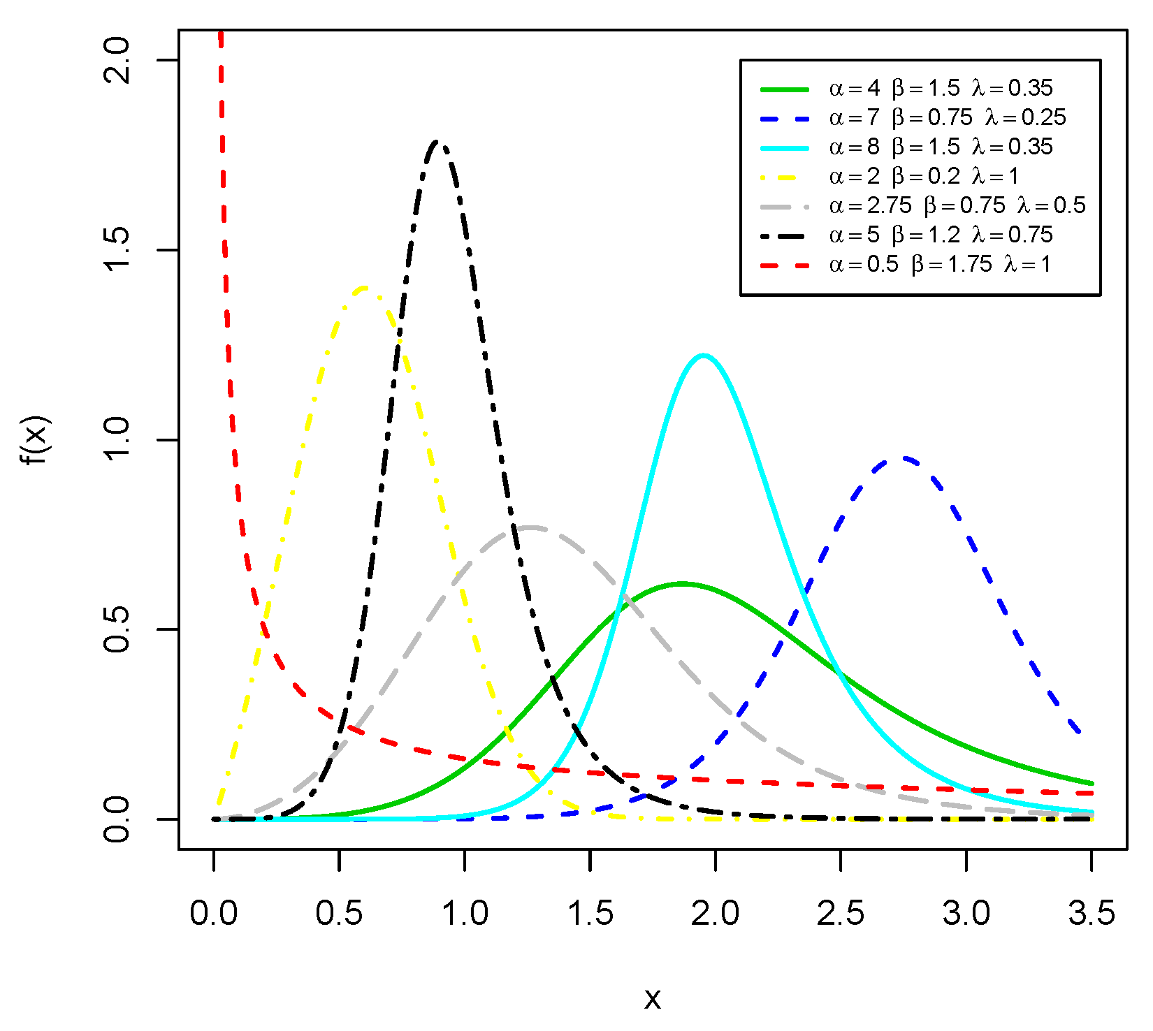
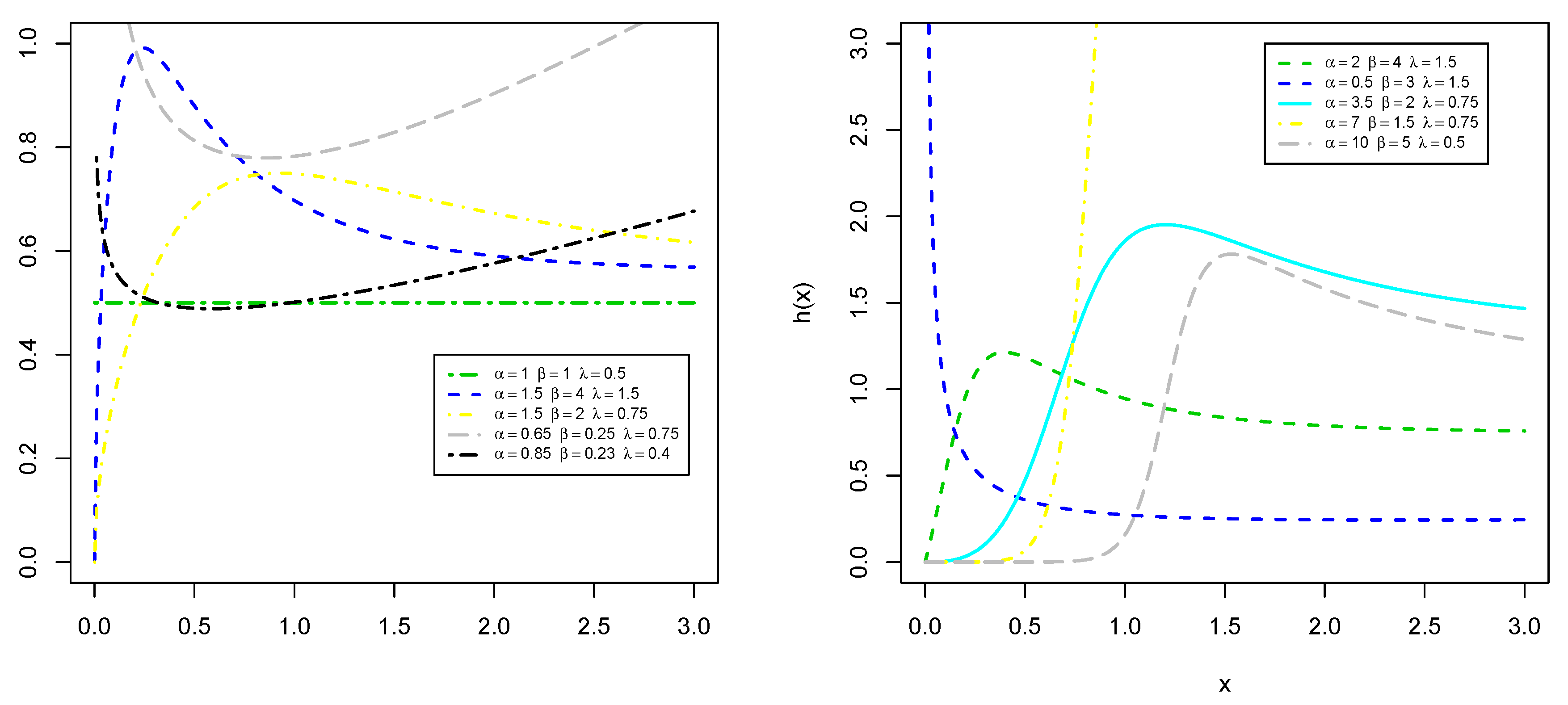
Figure 1 and Figure 2 display some possible shapes of the PDF and HRF of the EOWEx distribution. These figures indicate that the PDF of the EOWEx distribution can be left-skewed, right-skewed, reversed-J shaped, and symmetric. Further, the HRF of the EOWEx distribution has some important shapes, including constant, increasing, decreasing, upside down bathtub, reversed bathtub, reversed-J shaped, which are desirable characteristics for a lifetime distribution. It can be seen, from the application section, that the EOWEx distribution allows greater flexibility and can be used to model skewed data and can be widely applied in different areas such as reliability, biomedical studies, biology, engineering, and survival analysis.
3. Some Properties
In this section, we obtain some properties of the EOWEx distribution including the linear representation, moments, moment generating function (MGF), mean residual life, mean inactivity time, and order statistics.
3.1. Linear Representation
We provide a useful linear representation for the EOWEx density. Alizadeh et al. [10] derived a mixture representation of the EOW-G density as follows,
where and is the Exp-G density with positive power parameter . Using the PDF and CDF of the Ex distribution, the last equation can be rewritten as
Applying the binomial expansion to , the above equation reduces to
Equation (7) can be expressed as
where
and denotes the Ex density with scale parameter . Then, the EOWEx PDF can be expressed as a single linear combination of Ex densities. Let Z be a random variable having the Ex distribution with PDF , , . Then, the rth ordinary and incomplete moments, and MGF of Z are
respectively, where is the gamma function and is the lower incomplete gamma function.
3.2. Moments and MGF
Table 1 displays the numerical values of the mean (), variance (), skewness (), and kurtosis () of the EOWEx distribution for and some selected values of and . The values in Table 1 illustrate that the skewness of the EOWEx distribution is ranging in the interval (, ), whereas the spread of its kurtosis is much larger ranging from to . Furthermore, the EOWEx distribution can be left skewed or right skewed, and it can be leptokurtic (). Therefore, the EOWEx distribution can be used to model the skewed data due to its flexibility.
The first incomplete moment of X follows from the last equation as
Based on Equation (8), the MGF of the EOWEx distribution takes the form
3.3. Mean Residual Life and Mean Inactivity Time
The mean residual life (MRL) (also known as the life expectancy at age t) represents the expected additional life length for a unit, which is alive at age t and is defined by
The MRL of X is
where is given by (10) and is the SF of the EOWEx distribution. Inserting Equation (10) in (11), we have
The mean inactivity time (MIT) is defined by (for ) and it represents the waiting time elapsed since the failure of an item on condition that this failure had occurred in .
The MIT of X is
3.4. Order Statistics
Order statistics are important in many areas of statistical theory and practice. According to Alizadeh et al. [10], the PDF of ith order statistic of the EOW-G class, (for ), can be expressed as
Here, is the exponentiated exponential density with power parameter and
Let be a random sample from the EOWEx model and let be the associated order statistics. The PDF of ith order statistic reduces to
Applying the binomial series, the last equation becomes
where
Equation (14) means that the PDF of EOWEx order statistics is a mixture of Ex densities with scale parameter . Therefore, some of their mathematical properties are obtained from those of the Ex distribution. For example, the qth moments of is
4. Estimation Methods
In this section, we study the estimation problem of the EOWEx parameters using eight different estimation methods called: the maximum likelihood estimators (MLEs), least squares estimators (LSEs), weighted least-squares estimators (WLSEs), maximum product of spacing estimators (MPSEs), percentiles estimators (PCEs), Cramér-von Mises estimators (CMEs), Anderson-Darling estimators (ADEs), and right-tail Anderson-Darling estimators (RTADEs).
4.1. Maximum Likelihood Method
Let be a random sample from the EOWEx distribution with parameters , and . The log-likelihood function has the form
where . The MLEs of , and can be obtained by maximizing the last equation with respect to , and , or by solving the following nonlinear equations,
and
The R (optim function), Ox program (sub-routine MaxBFGS), SAS (PROCNLMIXED), Mathcad program, or Newton–Rapshon method can be used to maximize the log-likelihood function to obtain the MLEs. The log-likelihood is maximized using a wide range of starting values. The starting values were taken to correspond to all combinations of the model parameters, where = 0.1, 0.5, …, 10, = 0.1, 0.5, …, 10 and = 0.1, 0.5, …, 10. The call to optim converged about 98 percent of the time. The maximum likelihood solution was unique, when the calls to optim did converge. The elements of the observed information matrix are given in explicit expressions as follows,
and
4.2. Least Squares and Weighted Least Squares Methods
The least squares (LS) and weighted least square (WLS) methods are used to estimate the parameters of the beta distribution (Swain et al. [11]). Let be the sample order statistics of size n from the EOWEx distribution; therefore, the LS estimators (LSEs) and WLS estimators (WLSEs) of the EOWEx parameters , and can be obtained by minimizing
with respect to , , and , where in case of LSEs and in case of WLSEs. Furthermore, the LSEs and WLSEs follow by solving the nonlinear equations
where
4.3. Maximum Product of Spacings Method
The maximum product of spacings (MPS) method is used to estimate the parameters of continuous univariate models as an alternative to the ML method (Cheng and Amin, [12,13]). The uniform spacings of a random sample of size n from the EOWEx distribution can be defined by
where denotes to the uniform spacings, , and . The MPS estimators (MPSEs) of the EOWEx parameters can be obtained by maximizing
with respect to , , and . Further, the MPSEs of the EOWEx parameters can also be obtained by solving
where , (for ) is defined by (15).
4.4. Percentile Method
Here, we use the percentile method (Kao, [14]) to estimate the unknown parameters of the EOWEx distribution by equating the sample percentile points with the population percentile points. Let be an unbiased estimator of . Then, the percentile estimators (PCEs) of the EOWEx parameters are obtained by minimizing the following function with respect to , , and ,
4.5. Cramér-von-Mises Method
The Cramér-von-Mises estimators (CVMEs) (Cramér [15]; von Mises [16]) can be obtained based on the difference between the estimates of the CDF and the empirical distribution function (Luceño, [17]). The CVMEs of the EOWEx parameters , and are obtained by minimizing the following function with respect to , , and ,
Further, the CVMEs follow by solving the nonlinear equations
where , (for ) is defined by Equation (15).
4.6. Anderson-Darling and Right-Tail Anderson-Darling Methods
The Anderson-Darling estimators (ADEs) are another type of minimum distance estimators. The ADEs of the EOWEx parameters are obtained by minimizing
with respect to , , and . The ADEs can also be obtained by solving the nonlinear equations
where , (for ) is defined by (15). The right-tail Anderson-Darling estimators (RTADEs) of the EOWEx parameters , and are obtained by minimizing the following function with respect to , and ,
5. Simulation Results
In this section, the performance of eight different estimators of the EOWEx parameters is assessed by a simulation study. We consider different sample sizes , 50, for different parameters values , , , , and , . We generate random samples from EOWEx distribution. For each estimate, we obtain the average values of the estimates (AEs) and their corresponding mean squares error (MSEs).
The performance of different estimators are evaluated in terms of MSEs, i.e., the most efficient estimation method will be the one whose MSEs values are closer to zero. The simulation results are obtained via the R software. Table 2, Table 3 and Table 4 show the AEs and MSEs (in parentheses) of the MLEs, LSEs, WLSEs, MPSEs, PCEs, CVMEs, ADEs, and RTADEs. Further, the AEs based on all estimation methods tend to the true parameter values, as the sample size increase in all cases, which indicates that all estimators are asymptotically unbiased. The figures in these tables means that MLEs, LSEs, WLSEs, MPSEs, PCEs, CVMEs, ADEs, and RTADEs perform very well, in terms of MSEs, for estimating the EOWEx parameters.
6. Applications in Medicine, Engineering, and Reliability
In this section, the EOWEx distribution is fitted to four data sets from fields of medicine, engineering, and reliability. The EOWEx model is compared with other some competitive models called, the exponentiated exponential (EEx) (Gupta and Kundu, [2]), beta exponential (BEx) (Nadarajah and Kotz, [18]), alpha power exponential (APEx) (Mahdavi and Kundu, [19]), and exponential (Ex) distributions. The densities of these models are given by
EEx:
BEx:
MOEx:
APEx:
The fit of these distributions is evaluated using some measures including Cramér-von Mises (), Anderson-Darling (), and Kolmogorov Smirnov (KS) statistics with its p-value.
The first set of data was studied by Lee and Wang [20], and it represents the remission times (in months) of a random sample of 128 bladder cancer patients. These data were analyzed by Sen et al. [21], Afify et al. [22], and Mansour et al. [23]. The second set of data was studied by Kundu and Raqab [24], and it represents the gauge lengths of 20 mm of a sample of 74 observations. This data set was analyzed by Afify et al. [25] and Afify et al. [26]. The third set of data consists of the failure times of 20 mechanical components (Murthy et al. [27]). The fourth set of data refers to breaking stress of carbon fibres (in Gba) and it consists of 100 observations (Nichols and Padgett, [28]). These data were analyzed by Afify et al. [29].
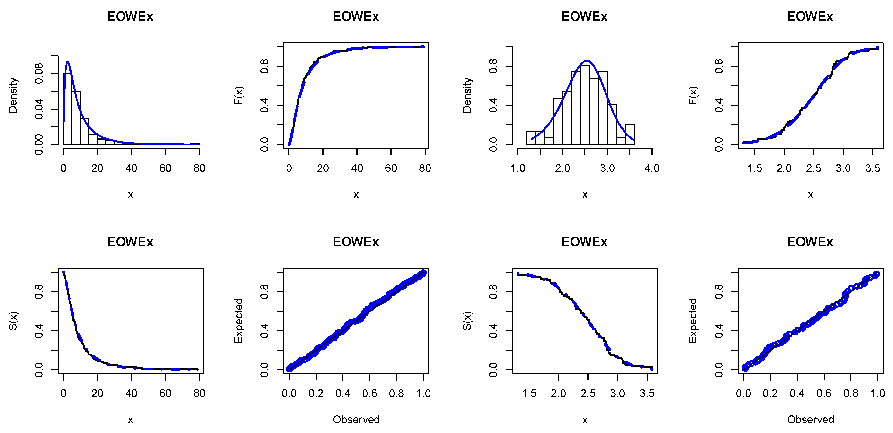
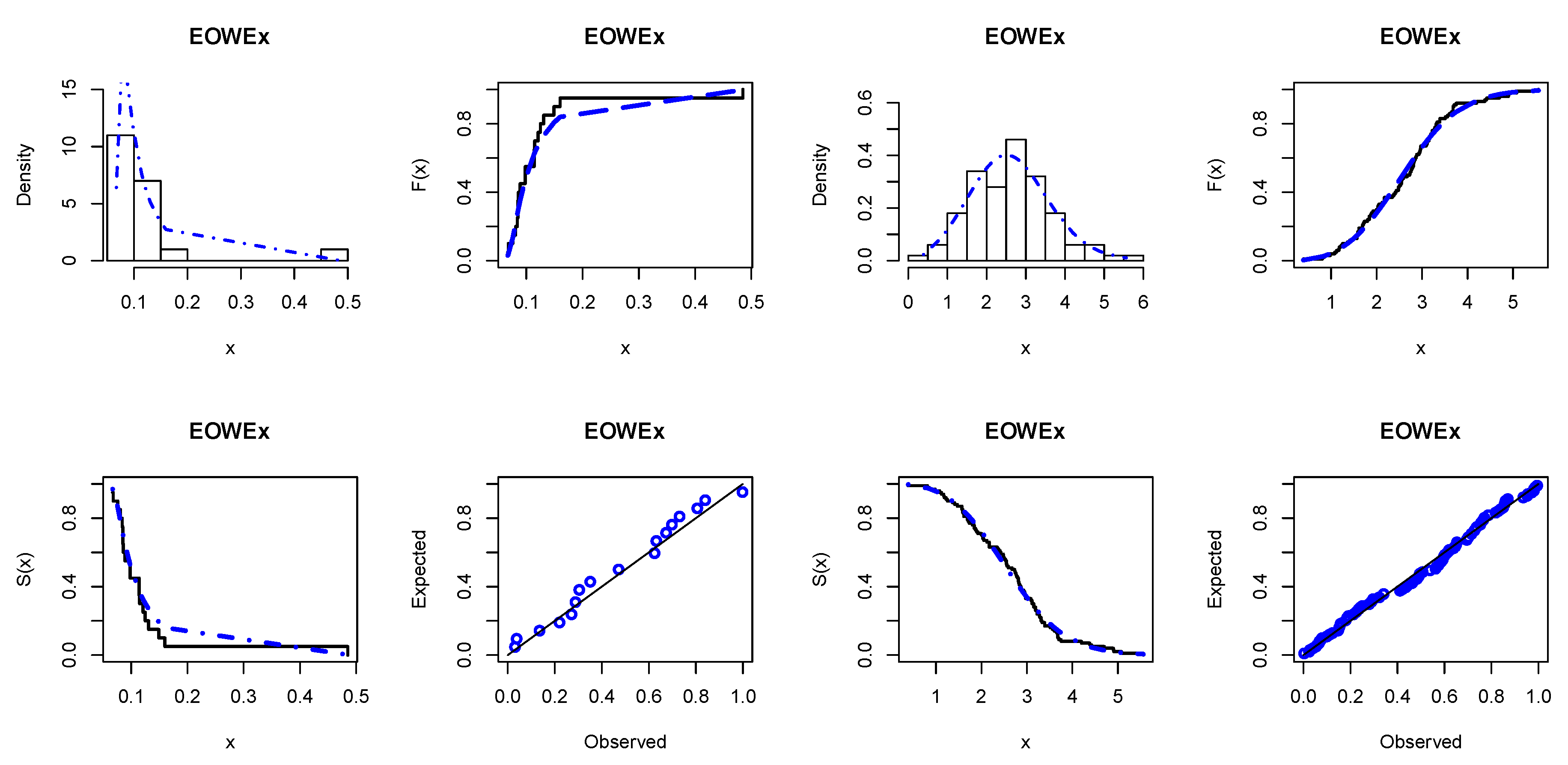
Table 5, Table 6, Table 7 and Table 8 provide the values of , , and KS as well as the p-value for the models fitted to the four data sets, respectively. Further, Table 5, Table 6, Table 7 and Table 8 display the MLEs and standard errors (SEs) (appear in parentheses) of the parameters of the EOWEx, EEx, BEx, APEx, and Ex models. In Table 5, Table 6, Table 7 and Table 8, we compare the fits of the EOWEx model with the EEx, BEx, APEx, and Ex models. The figures in these tables indicate that the EOWEx distribution has the lowest values of , , KS and largest p-value, among all fitted models. The fitted EOWEx PDF, CDF, SF, and P–P plots of the four data sets are displayed in Figure 3 and Figure 4, respectively.
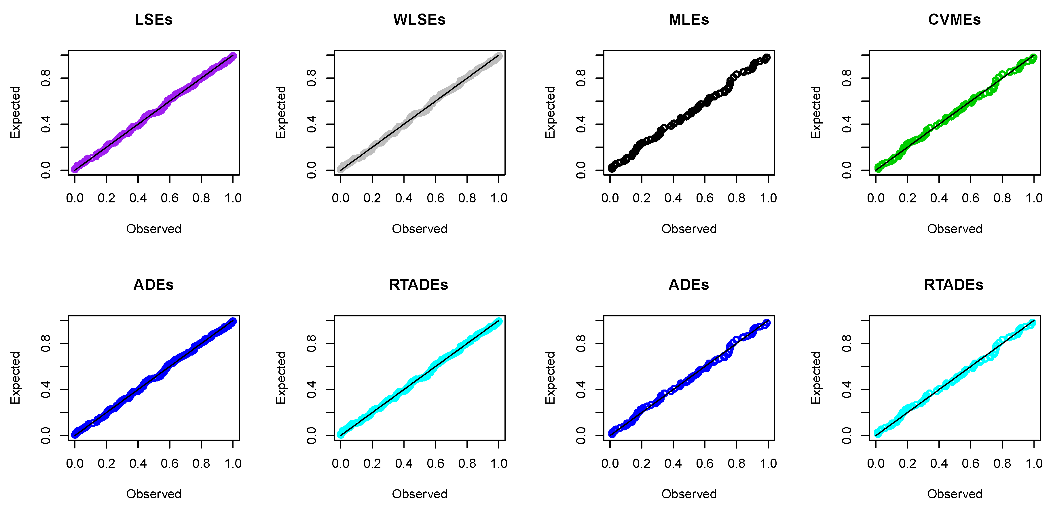
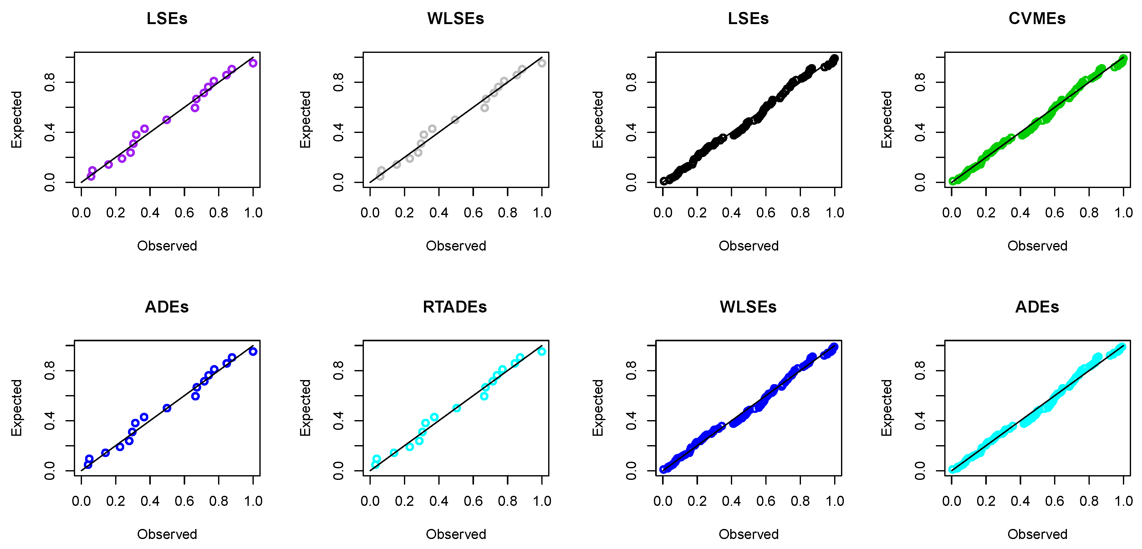
Furthermore, we use the eight estimation methods discussed in Section 4 to estimate the EOWEx parameters. Table 9, Table 10, Table 11 and Table 12 display the estimates of the EOWEx parameters using these estimation methods and the numerical values of KS and its p-value for the four data sets, respectively. Based on the values of KS and p-value, in Table 9, Table 10, Table 11 and Table 12, the LSEs is recommended to estimate the EOWEx parameters for cancer data, failure times data, and breaking stress of carbon fibers data, whereas the MLEs is recommended to estimate the EOWEx parameters for gauge lengths data. However, all estimation methods perform very well for the four data sets. The P–P plots of the EOWEx distribution using the four best estimation methods are displayed in Figure 5 and Figure 6, for the four data sets, respectively.
7. Concluding Remarks
In this paper, we propose the three-parameter extended odd Weibull exponential (EOWEx) distribution. The EOWEx density is a linear combination of exponential densities. Some of its mathematical properties are obtained. The EOWEx parameters are estimated by eight different estimation methods called, MLEs, LSEs, WLSEs, MPSEs, PCEs, CVMES, ADEs, and RTADEs. An extensive simulation study is conducted to compare the performance of these different estimators to identify the best performing estimators. The simulation results reveal that all estimators perform very well in terms of their mean square errors. Four real data applications are used to prove the EOWEx flexibility and potentiality. These applications show that the EOWEx model can yield better fits than some other existing extensions of the exponential distribution. We expect the utility of the newly proposed model in several fields such as reliability, medicine, engineering, and life testing.
Author Contributions
A.Z.A. and O.A.M. contributed equally to this work. All authors have read and agreed to the published version of the manuscript.
Funding
This research received no external funding.
Acknowledgments
The authors would like to thank the four anonymous reviewers for their very constructive comments and suggestions which greatly improved the final version of the manuscript.
Conflicts of Interest
The authors declare no conflict of interest.
References
- Marshall, A.W.; Olkin, I. A new method for adding a parameter to a family of distributions with application to the exponential and Weibull families. Biometrika 1997, 84, 641–652. [Google Scholar] [CrossRef]
- Gupta, R.D.; Kundu, D. Exponentiated exponential family: An alternative to gamma and Weibull distributions. Biom. J. J. Math. Methods Biosci. 2001, 43, 117–130. [Google Scholar] [CrossRef]
- Pinho, L.G.B.; Cordeiro, G.M.; Nobre, J.S. The Harris extended exponential distribution. Commun. Stat. Theory Methods 2015, 44, 3486–3502. [Google Scholar] [CrossRef]
- Afify, A.Z.; Cordeiro, G.M.; Yousof, H.M.; Alzaatreh, A.; Nofal, Z.M. The Kumaraswamy transmuted-G family of distributions: Properties and applications. J. Data Sci. 2016, 14, 245–270. [Google Scholar]
- Rasekhi, M.; Alizadeh, M.; Altun, E.; Hamedani, G.G.; Afify, A.Z.; Ahmad, M. The modified exponential distribution with applications. Pak. J. Stat. 2017, 33, 383–398. [Google Scholar]
- Afify, A.Z.; Zayed, M.; Ahsanullah, M. The extended exponential distribution and its applications. J. Stat. Theory Appl. 2018, 17, 213–229. [Google Scholar] [CrossRef] [Green Version]
- Mansour, M.M.; Abd Elrazik, E.M.; Afify, A.Z.; Ahsanullah, M.; Altun, E. The transmuted transmuted-G family: Properties and applications. J. Nonlinear Sci. Appl. 2019, 12, 217–229. [Google Scholar] [CrossRef]
- Alizadeh, M.; Afify, A.Z.; Eliwa, M.S.; Ali, S. The odd log-logistic Lindley-G family of distributions: Properties, Bayesian and non-Bayesian estimation with applications. Comput. Stat. 2019. [Google Scholar] [CrossRef]
- Nassar, M.; Kumar, D.; Dey, S.; Cordeiro, G.M.; Afify, A.Z. The Marshall-Olkin alpha power family of distributions with applications. J. Comput. Appl. Math. 2019, 351, 41–53. [Google Scholar] [CrossRef]
- Alizadeh, M.; Altun, E.; Afify, A.Z.; Ozel, G. The extended odd Weibull-G family: Properties and applications. Commun. Fac. Sci. Univ. Ank. Ser. A1 Math. Stat. 2019, 68, 161–186. [Google Scholar] [CrossRef]
- Swain, J.; Venkatraman, S.; Wilson, J. Least squares estimation of distribution function in Johnsons translation system. J. Stat. Comput. Simul. 1988, 29, 271–297. [Google Scholar] [CrossRef]
- Cheng, R.; Amin, N. Maximum Product of Spacings Estimation with Application to the Lognormal Distribution (Mathematical Report 79-1); University of Wales IST: Cardiff, UK, 1979. [Google Scholar]
- Cheng, R.; Amin, N. Estimating parameters in continuous univariate distributions with a shifted origin. J. R. Stat. Soc. Ser. B-Stat. Methodol. 1983, 45, 394–403. [Google Scholar] [CrossRef]
- Kao, J.H.K. Computer methods for estimating Weibull parameters in reliability studies. IRE Trans. Reliab. Qual. Control 1958, 13, 15–22. [Google Scholar] [CrossRef]
- Cramér, H. On the composition of elementary errors. Scand. Actuar. J. 1928, 13–74. [Google Scholar] [CrossRef]
- Von Mises, R.E. Wahrscheinlichkeit Statistik und Wahrheit; Springer: Basel, Switzerland, 1928. [Google Scholar]
- Luceño, A. Fitting the generalized Pareto distribution to data using maximum goodness-of-fit estimators. Comput. Stat. Data Anal. 2006, 51, 904–917. [Google Scholar] [CrossRef]
- Nadarajah, S.; Kotz, S. The beta exponential distribution. Reliab. Eng. Syst. Saf. 2006, 91, 689–697. [Google Scholar] [CrossRef]
- Mahdavi, A.; Kundu, D. A new method for generating distributions with an application to exponential distribution. Commun. Stat. Theory Methods 2017, 46, 6543–6557. [Google Scholar] [CrossRef]
- Lee, E.T.; Wang, J.W. Statistical Methods for Survival Data Analysis, 3rd ed.; John Wiley and Sons, Inc.: Hoboken, NJ, USA, 2003. [Google Scholar]
- Sen, S.; Afify, A.Z.; Al-Mofleh, H.; Ahsanullahd, M. The quasi xgamma-geometric distribution with application in medicine. Filomat 2019, 33, 5291–5330. [Google Scholar]
- Afify, A.Z.; Suzuki, A.K.; Zhang, C.; Nassar, M. On three-parameter exponential distribution: Properties, Bayesian and non-Bayesian estimation based on complete and censored samples. Commun. Stat. Simul. Comput. 2019. [Google Scholar] [CrossRef]
- Mansoor, M.; Tahir, M.H.; Cordeiro, G.M.; Provost, S.B.; Alzaatreh, A. The Marshall-Olkin logistic-exponential distribution. Commun. Stat. Theory Methods 2019, 48, 220–234. [Google Scholar] [CrossRef]
- Kundu, D.; Raqab, M.Z. Estimation of R = P(Y < X) for three parameter Weibull distribution. Stat. Probab. Lett. 2009, 79, 1839–1846. [Google Scholar]
- Afify, A.Z.; Cordeiro, G.M.; Butt, N.S.; Ortega, E.M.; Suzuki, A.K. A new lifetime model with variable shapes for the hazard rate. Braz. J. Probab. Stat. 2017, 31, 516–541. [Google Scholar] [CrossRef]
- Afify, A.Z.; Cordeiro, G.M.; Bourguignon, M.; Ortega, E.M. Properties of the transmuted Burr XII distribution, regression and its applications. J. Data Sci. 2018, 16, 485–510. [Google Scholar]
- Murthy, D.P.; Xie, M.; Jiang, R. Weibull Models; John Wiley & Sons: Hoboken, NJ, USA, 2004. [Google Scholar]
- Nichols, M.D.; Padgett, W.J. A bootstrap control chart for Weibull percentiles. Qual. Reliab. Eng. Int. 2006, 22, 141–151. [Google Scholar] [CrossRef]
- Afify, A.Z.; Yousof, H.M.; Cordeiro, G.M.; Ortega, E.M.; Nofal, Z.M. The Weibull Fréchet distribution and its applications. J. Appl. Stat. 2016, 43, 2608–2626. [Google Scholar] [CrossRef]
Figure 1.
Plots of the probability density function (PDF) of the EOWEx distribution.

Figure 2.
Plots of the hazard rate function (HRF) of the EOWEx distribution.

Figure 3.
The fitted EOWEx PDF, CDF, SF, and P–P plots for cancer data (left panel) and for gauge lengths data (right panel).
Figure 3.
The fitted EOWEx PDF, CDF, SF, and P–P plots for cancer data (left panel) and for gauge lengths data (right panel).

Figure 4.
The fitted EOWEx PDF, CDF, SF, and P–P plots for failure times data (left panel) and for breaking stress of carbon fibers data (right panel).
Figure 4.
The fitted EOWEx PDF, CDF, SF, and P–P plots for failure times data (left panel) and for breaking stress of carbon fibers data (right panel).

Figure 5.
P–P plots of the EOWEx distribution using the four best estimation methods for cancer data (left panel) and for gauge lengths data (right panel).
Figure 5.
P–P plots of the EOWEx distribution using the four best estimation methods for cancer data (left panel) and for gauge lengths data (right panel).

Figure 6.
P-P plots of the EOWEx distribution using the four best estimation methods for failure times data (left panel) and for breaking stress of carbon fibers data (right panel).
Figure 6.
P-P plots of the EOWEx distribution using the four best estimation methods for failure times data (left panel) and for breaking stress of carbon fibers data (right panel).


Table 1.
The numerical values of , , and for the EOWEx distribution with .
| 0.5 | 0.5 | 1.07604 | 1.81240 | 1.86154 | 7.15518 |
| 1.5 | 2.14552 | 8.54064 | 2.24978 | 10.0097 | |
| 3 | 4.16961 | 31.8546 | 2.20377 | 9.41667 | |
| 5 | 7.00105 | 77.8477 | 1.77257 | 6.25858 | |
| 10 | 11.3657 | 160.743 | 1.12562 | 3.34256 | |
| 1.5 | 0.5 | 0.70607 | 0.19659 | 1.07999 | 4.86454 |
| 1.5 | 1.01631 | 0.80690 | 2.17662 | 10.5743 | |
| 3 | 1.63803 | 3.19461 | 2.42160 | 11.6298 | |
| 5 | 2.62656 | 9.50046 | 2.34542 | 10.9143 | |
| 10 | 5.41493 | 40.0672 | 2.04821 | 8.42506 | |
| 3 | 0.5 | 0.67367 | 0.05266 | 0.42752 | 3.64719 |
| 1.5 | 0.81058 | 0.17297 | 1.83271 | 9.57547 | |
| 3 | 1.08781 | 0.67101 | 2.49121 | 12.8818 | |
| 5 | 1.54272 | 2.08780 | 2.51062 | 12.3453 | |
| 10 | 2.88539 | 9.67645 | 2.30699 | 10.6753 | |
| 5 | 0.5 | 0.67418 | 0.02011 | 0.06681 | 3.48006 |
| 1.5 | 0.74998 | 0.05640 | 1.46409 | 8.07185 | |
| 3 | 0.90052 | 0.20413 | 2.41980 | 13.1505 | |
| 5 | 1.14971 | 0.64430 | 2.62182 | 13.6743 | |
| 10 | 1.90641 | 3.17554 | 2.45418 | 11.7785 | |
| 10 | 0.5 | 0.68077 | 0.00534 | -0.24265 | 3.69406 |
| 1.5 | 0.71589 | 0.01290 | 1.03088 | 6.32664 | |
| 3 | 0.78267 | 0.04096 | 2.11788 | 11.6589 | |
| 5 | 0.89108 | 0.12426 | 2.59860 | 14.4083 | |
| 10 | 1.22516 | 0.64424 | 2.67091 | 13.8583 |
Table 2.
The average values of the estimates (AEs) and mean squares errors (MSEs) for .
| Parameters | MLEs | LSEs | WLSEs | MPSEs | PCEs | CVMEs | ADEs | RTADEs |
|---|---|---|---|---|---|---|---|---|
| 3.692(0.410) | 3.406(0.427) | 3.428(0.407) | 3.256(0.417) | 3.949(0.202) | 3.627(0.434) | 3.525(0.391) | 3.582(0.421) | |
| 3.019(0.234) | 3.008(0.227) | 2.993(0.225) | 3.037(0.230) | 2.751(0.062) | 2.961(0.229) | 2.981(0.229) | 3.002(0.233) | |
| 1.005(0.017) | 1.013(0.019) | 1.010(0.018) | 1.008(0.017) | 1.125(0.026) | 1.000(0.018) | 1.004(0.017) | 1.002(0.019) | |
| 3.692(0.396) | 3.426(0.440) | 3.438(0.417) | 3.262(0.430) | 4.444(0.897) | 3.644(0.445) | 3.538(0.394) | 3.607(0.438) | |
| 2.991(0.232) | 2.990(0.230) | 2.961(0.226) | 3.014(0.230) | 2.517(0.246) | 2.940(0.229) | 2.960(0.227) | 2.992(0.233) | |
| 0.504(0.004) | 0.509(0.005) | 0.506(0.004) | 0.506(0.004) | 0.584(0.009) | 0.502(0.004) | 0.504(0.004) | 0.504(0.005) | |
| 3.678(0.547) | 3.481(0.532) | 3.501(0.521) | 3.377(0.514) | 3.949(0.201) | 3.649(0.550) | 3.590(0.514) | 3.646(0.553) | |
| 1.457(0.468) | 1.547(0.464) | 1.547(0.446) | 1.608(0.462) | 1.256(0.062) | 1.442(0.461) | 1.499(0.422) | 1.531(0.436) | |
| 0.991(0.013) | 1.004(0.013) | 1.002(0.013) | 1.006(0.013) | 1.016(0.010) | 0.993(0.013) | 0.996(0.012) | 0.997(0.013) | |
| 3.647(0.559) | 3.446(0.534) | 3.455(0.527) | 3.350(0.529) | 3.946(0.201) | 3.621(0.554) | 3.553(0.526) | 3.580(0.540) | |
| 1.422(0.500) | 1.536(0.495) | 1.514(0.471) | 1.570(0.474) | 1.262(0.062) | 1.440(0.501) | 1.476(0.454) | 1.486(0.467) | |
| 0.495(0.004) | 0.503(0.003) | 0.501(0.003) | 0.502(0.003) | 0.525(0.006) | 0.497(0.003) | 0.498(0.003) | 0.498(0.004) | |
| 0.792(0.025) | 0.749(0.028) | 0.755(0.026) | 0.706(0.024) | 1.053(0.089) | 0.797(0.031) | 0.771(0.025) | 0.790(0.030) | |
| 0.237(0.014) | 0.281(0.016) | 0.280(0.016) | 0.273(0.016) | 0.159(0.010) | 0.274(0.017) | 0.279(0.018) | 0.282(0.016) | |
| 0.530(0.016) | 0.533(0.020) | 0.533(0.019) | 0.529(0.016) | 0.662(0.038) | 0.539(0.021) | 0.536(0.019) | 0.534(0.019) |
Table 3.
The AEs and MSEs for .
| Parameters | MLEs | LSEs | WLSEs | MPSEs | PCEs | CVMEs | ADEs | RTADEs |
|---|---|---|---|---|---|---|---|---|
| 3.650(0.270) | 3.500(0.276) | 3.528(0.254) | 3.386(0.256) | 3.949(0.202) | 3.603(0.285) | 3.557(0.248) | 3.582(0.254) | |
| 3.058(0.222) | 3.014(0.219) | 3.014(0.218) | 3.027(0.216) | 2.751(0.062) | 2.999(0.218) | 3.014(0.218) | 3.037(0.223) | |
| 1.005(0.008) | 1.006(0.008) | 1.004(0.008) | 1.002(0.007) | 1.158(0.025) | 1.101(0.008) | 1.002(0.008) | 1.004(0.009) | |
| 3.627(0.254) | 3.494(0.281) | 3.511(0.248) | 3.355(0.242) | 3.949(0.201) | 3.598(0.290) | 3.544(0.240) | 3.575(0.261) | |
| 3.046(0.223) | 3.010(0.218) | 3.004(0.213) | 3.007(0.215) | 2.751(0.062) | 2.995(0.216) | 3.005(0.215) | 3.030(0.227) | |
| 0.502(0.002) | 0.502(0.002) | 0.502(0.002) | 0.500(0.002) | 0.568(0.008) | 0.500(0.002) | 0.501(0.002) | 0.501(0.002) | |
| 3.600(0.404) | 3.517(0.430) | 3.537(0.411) | 3.421(0.375) | 3.949(0.200) | 3.592(0.435) | 3.571(0.395) | 3.610(0.490) | |
| 1.509(0.338) | 1.526(0.371) | 1.538(0.339) | 1.568(0.325) | 1.251(0.062) | 1.489(0.366) | 1.524(0.321) | 1.546(0.363) | |
| 0.995(0.006) | 0.998(0.007) | 0.998(0.006) | 1.000(0.006) | 1.036(0.006) | 0.994(0.007) | 0.997(0.006) | 0.997(0.007) | |
| 3.601(0.407) | 3.512(0.412) | 3.518(0.394) | 3.423(0.381) | 3.929(0.202) | 3.593(0.423) | 3.570(0.390) | 3.615(0.481) | |
| 1.513(0.354) | 1.533(0.403) | 1.528(0.365) | 1.571(0.339) | 1.251(0.062) | 1.502(0.399) | 1.531(0.341) | 1.558(0.379) | |
| 0.499(0.002) | 0.501(0.002) | 0.500(0.002) | 0.502(0.002) | 0.520(0.004) | 0.499(0.002) | 0.500(0.002) | 0.501(0.002) | |
| 0.774(0.011) | 0.757(0.013) | 0.762(0.012) | 0.731(0.010) | 1.048(0.085) | 0.779(0.014) | 0.768(0.012) | 0.775(0.013) | |
| 0.257(0.014) | 0.282(0.016) | 0.287(0.016) | 0.290(0.016) | 0.152(0.010) | 0.281(0.016) | 0.285(0.016) | 0.290(0.016) | |
| 0.513(0.008) | 0.520(0.011) | 0.521(0.010) | 0.518(0.008) | 0.645(0.033) | 0.523(0.011) | 0.521(0.010) | 0.522(0.010) |
Table 4.
The AEs and MSEs for .
| Parameters | MLEs | LSEs | WLSEs | MPSEs | PCEs | CVMEs | ADEs | RTADEs |
|---|---|---|---|---|---|---|---|---|
| 3.556(0.163) | 3.487(0.189) | 3.496(0.163) | 3.384(0.163) | 3.948(0.201) | 3.541(0.192) | 3.509(0.159) | 3.531(0.183) | |
| 3.016(0.198) | 3.003(0.207) | 2.995(0.195) | 2.970(0.192) | 2.758(0.060) | 2.997(0.205) | 2.993(0.195) | 3.002(0.213) | |
| 1.002(0.004) | 1.002(0.004) | 1.001(0.004) | 0.997(0.004) | 1.069(0.024) | 0.999(0.004) | 1.000(0.004) | 0.999(0.005) | |
| 3.588(0.181) | 3.505(0.198) | 3.519(0.176) | 3.417(0.172) | 3.949(0.201) | 3.559(0.205) | 3.534(0.174) | 3.549(0.190) | |
| 3.038(0.200) | 3.012(0.209) | 3.006(0.200) | 2.995(0.196) | 2.751(0.062) | 3.007(0.210) | 3.007(0.199) | 3.013(0.208) | |
| 0.502(0.001) | 0.502(0.001) | 0.501(0.001) | 0.500(0.001) | 0.489(0.005) | 0.500(0.001) | 0.501(0.001) | 0.500(0.001) | |
| 3.568(0.267) | 3.513(0.331) | 3.524(0.280) | 3.456(0.242) | 3.949(0.198) | 3.557(0.335) | 3.543(0.270) | 3.579(0.365) | |
| 1.522(0.231) | 1.516(0.305) | 1.523(0.249) | 1.552(0.219) | 1.251(0.062) | 1.504(0.303) | 1.521(0.236) | 1.537(0.270) | |
| 1.000(0.004) | 0.999(0.004) | 1.000(0.004) | 1.002(0.004) | 1.048(0.005) | 0.997(0.004) | 0.999(0.004) | 0.999(0.004) | |
| 3.587(0.275) | 3.530(0.321) | 3.544(0.282) | 3.476(0.248) | 3.919(0.198) | 3.573(0.326) | 3.564(0.275) | 3.596(0.363) | |
| 1.535(0.230) | 1.533(0.298) | 1.541(0.248) | 1.565(0.219) | 1.251(0.062) | 1.521(0.294) | 1.536(0.236) | 1.551(0.271) | |
| 0.501(0.001) | 0.501(0.001) | 0.501(0.001) | 0.502(0.001) | 0.514(0.001) | 0.500(0.001) | 0.501(0.001) | 0.501(0.001) | |
| 0.764(0.006) | 0.755(0.007) | 0.758(0.006) | 0.742(0.005) | 1.045(0.080) | 0.766(0.008) | 0.761(0.006) | 0.767(0.008) | |
| 0.255(0.013) | 0.275(0.015) | 0.273(0.014) | 0.288(0.015) | 0.151(0.010) | 0.275(0.015) | 0.273(0.014) | 0.278(0.015) | |
| 0.509(0.005) | 0.513(0.006) | 0.513(0.006) | 0.517(0.005) | 0.635(0.030) | 0.515(0.006) | 0.514(0.006) | 0.514(0.006) |
Table 5.
The , , KS, p-value, MLEs, and SEs for cancer data.
| Distribution | KS | p-Value | Estimates (SEs) | |||
|---|---|---|---|---|---|---|
| EOWEx | 0.0390 | 0.2597 | 0.0445 | 0.9617 | 1.4434(0.1992) | |
| 1.9774(0.6451) | ||||||
| 0.1306(0.0214) | ||||||
| EEx | 0.1122 | 0.6741 | 0.0725 | 0.5113 | 1.2179(0.1488) | |
| 0.1212(0.0136) | ||||||
| BEx | 0.1195 | 0.7168 | 0.0733 | 0.4980 | a | 1.1752(0.1318) |
| b | 5.0822(8.0755) | |||||
| 0.0243(0.0381) | ||||||
| APEx | 0.1283 | 0.7672 | 0.0793 | 0.3963 | 1.1744(0.8437) | |
| 0.1113(0.0226) | ||||||
| Ex | 0.1193 | 0.7160 | 0.0846 | 0.3184 | 0.1068(0.0094) | |
Table 6.
The , , KS, p-value, MLEs, and SEs for gauge lengths data.
| Distribution | KS | p-Value | Estimates (SEs) | |||
|---|---|---|---|---|---|---|
| EOWEx | 0.0245 | 0.1831 | 0.0509 | 0.9908 | 4.9821(0.7601) | |
| 0.3111(0.2597) | ||||||
| 0.2674(0.0086) | ||||||
| EEx | 0.2172 | 1.4053 | 0.0953 | 0.5121 | 89.435(32.476) | |
| 2.0192(0.1716) | ||||||
| BEx | 0.0874 | 0.5738 | 0.0682 | 0.8809 | a | 24.317(3.9884) |
| b | 92.491(154.90) | |||||
| 0.0947(0.1426) | ||||||
| APEx | 0.1153 | 0.7486 | 0.1924 | 0.0083 | 1592046(16777) | |
| 1.2536(0.0549) | ||||||
| Ex | 0.0876 | 0.5749 | 0.4495 | 0.0000 | 0.4037(0.0469) | |
Table 7.
The , , KS, p-value, MLEs, and SEs for failure times data.
| Distribution | KS | p-Value | Estimates (SEs) | |||
|---|---|---|---|---|---|---|
| EOWEx | 0.0586 | 0.4551 | 0.1193 | 0.9383 | 12.261(7.5036) | |
| 8.2078(6.5143) | ||||||
| 8.4547(0.9487) | ||||||
| EEx | 0.1758 | 1.2510 | 0.1603 | 0.6831 | 13.825(8.3755) | |
| 27.752(6.1078) | ||||||
| BEx | 0.1826 | 1.2759 | 0.1624 | 0.6672 | a | 2056.2(4396.0) |
| b | 0.1723(0.0730) | |||||
| 113.18(34.244) | ||||||
| APEx | 0.1799 | 1.2755 | 0.1602 | 0.6834 | 22078970(23726) | |
| 29.463(2.3335) | ||||||
| Ex | 0.2912 | 1.9025 | 0.4238 | 0.0015 | 8.2271(1.8396) | |
Table 8.
The , , KS, p-value, MLEs, and SEs for breaking stress of carbon fibres data.
| Distribution | KS | p-Value | Estimates (SEs) | |||
|---|---|---|---|---|---|---|
| EOWEx | 0.0620 | 0.3670 | 0.0626 | 0.8286 | 2.4872(0.3193) | |
| 0.3789(0.2345) | ||||||
| 0.2517(0.0143) | ||||||
| EEx | 0.2267 | 1.1859 | 0.1077 | 0.1962 | 7.7882(1.4961) | |
| 1.0132(0.0874) | ||||||
| BEx | 0.1483 | 0.7588 | 0.0935 | 0.3461 | a | 5.9605(0.8217) |
| b | 34.546(61.141) | |||||
| 0.0615(0.1021) | ||||||
| APEx | 0.1792 | 0.9118 | 0.0961 | 0.3139 | 19134.8(8983) | |
| 1.0777(0.0509) | ||||||
| Ex | 0.1493 | 0.7643 | 0.3206 | 0.0000 | 0.3815(0.0381) | |
Table 9.
The estimates of the EOWEx parameters, KS and p-value for cancer data.
| Method | KS | p-Value | |||
|---|---|---|---|---|---|
| MLEs | 1.4434 | 1.9774 | 0.1306 | 0.0445 | 0.9617 |
| LSEs | 1.5585 | 2.1115 | 0.1364 | 0.0297 | 0.9999 |
| WLSEs | 1.5055 | 2.0333 | 0.1347 | 0.0302 | 0.9998 |
| MPSEs | 1.3593 | 1.8593 | 0.1266 | 0.0545 | 0.8414 |
| PCEs | 1.5444 | 3.2551 | 0.1752 | 0.0653 | 0.6466 |
| CVMEs | 1.5774 | 2.1054 | 0.1360 | 0.0305 | 0.9998 |
| ADEs | 1.5020 | 2.0006 | 0.1338 | 0.0299 | 0.9998 |
| RTADEs | 1.7470 | 2.6811 | 0.1485 | 0.0337 | 0.9986 |
Table 10.
The estimates of the EOWEx parameters, KS and p-value for gauge lengths data.
| Method | KS | p-Value | |||
|---|---|---|---|---|---|
| MLEs | 4.9821 | 0.3111 | 0.2674 | 0.0509 | 0.9908 |
| LSEs | 4.5195 | 0.1217 | 0.2628 | 0.0562 | 0.9735 |
| WLSEs | 4.7775 | 0.2655 | 0.2663 | 0.0559 | 0.9751 |
| MPSEs | 4.8804 | 0.3746 | 0.2688 | 0.0593 | 0.9572 |
| PCEs | 4.8023 | 0.3481 | 0.2681 | 0.0611 | 0.9452 |
| CVMEs | 4.5925 | 0.1116 | 0.2628 | 0.0512 | 0.9901 |
| ADEs | 4.8986 | 0.2922 | 0.2669 | 0.0530 | 0.9856 |
| RTADEs | 5.0533 | 0.3383 | 0.2678 | 0.0512 | 0.9900 |
Table 11.
The estimates of the EOWEx parameters, KS and p-value for failure times data.
| Method | KS | p-Value | |||
|---|---|---|---|---|---|
| MLEs | 12.261 | 8.2078 | 8.4547 | 0.1193 | 0.9383 |
| LSEs | 8.2758 | 4.6100 | 8.1032 | 0.1115 | 0.9649 |
| WLSEs | 7.6719 | 3.9912 | 7.9537 | 0.1166 | 0.9484 |
| MPSEs | 9.6030 | 7.3144 | 8.3930 | 0.1561 | 0.7143 |
| PCEs | 8.8209 | 11.152 | 10.809 | 0.2360 | 0.2151 |
| CVMEs | 10.031 | 5.3648 | 8.1602 | 0.1221 | 0.9267 |
| ADEs | 9.9942 | 5.5882 | 8.2107 | 0.1144 | 0.9560 |
| RTADEs | 11.981 | 7.0147 | 8.4120 | 0.1138 | 0.9579 |
Table 12.
The estimates of the EOWEx parameters, KS and p-value for breaking stress of carbon fibres data.
Table 12.
The estimates of the EOWEx parameters, KS and p-value for breaking stress of carbon fibres data.
| Method | KS | p-Value | |||
|---|---|---|---|---|---|
| MLEs | 2.4872 | 0.3789 | 0.2517 | 0.0628 | 0.8286 |
| LSEs | 2.0913 | 0.0489 | 0.2369 | 0.0524 | 0.9725 |
| WLSEs | 2.3597 | 0.2562 | 0.2467 | 0.0587 | 0.9301 |
| MPSEs | 2.2562 | 0.4245 | 0.2536 | 0.0653 | 0.8619 |
| PCEs | 2.3148 | 0.4696 | 0.2556 | 0.0661 | 0.8531 |
| CVMEs | 2.1166 | 0.0222 | 0.2362 | 0.0540 | 0.9640 |
| ADEs | 2.2854 | 0.3545 | 0.2504 | 0.0613 | 0.9060 |
| RTADEs | 2.5169 | 0.5115 | 0.2562 | 0.0633 | 0.8859 |
© 2020 by the authors. Licensee MDPI, Basel, Switzerland. This article is an open access article distributed under the terms and conditions of the Creative Commons Attribution (CC BY) license (http://creativecommons.org/licenses/by/4.0/).
Share and Cite
MDPI and ACS Style
Afify, A.Z.; Mohamed, O.A. A New Three-Parameter Exponential Distribution with Variable Shapes for the Hazard Rate: Estimation and Applications. Mathematics 2020, 8, 135. https://0-doi-org.brum.beds.ac.uk/10.3390/math8010135
AMA Style
Afify AZ, Mohamed OA. A New Three-Parameter Exponential Distribution with Variable Shapes for the Hazard Rate: Estimation and Applications. Mathematics. 2020; 8(1):135. https://0-doi-org.brum.beds.ac.uk/10.3390/math8010135
Chicago/Turabian StyleAfify, Ahmed Z., and Osama Abdo Mohamed. 2020. "A New Three-Parameter Exponential Distribution with Variable Shapes for the Hazard Rate: Estimation and Applications" Mathematics 8, no. 1: 135. https://0-doi-org.brum.beds.ac.uk/10.3390/math8010135
Note that from the first issue of 2016, this journal uses article numbers instead of page numbers. See further details here.