Nash Equilibrium Investment-Reinsurance Strategies for an Insurer and a Reinsurer with Intertemporal Restrictions and Common Interests

Abstract

This paper investigates the generalized multi-period mean-variance investment-reinsurance optimization model in a discrete-time framework for a general insurance company that contains a reinsurer and an insurer. The intertemporal restrictions and the common interests of the reinsurer and the insurer are considered. The common goal of the reinsurer and the insurer is to maximize the expectation of the weighted sum of their wealth processes and minimize the corresponding variance. Based on the game method, we obtain the Nash equilibrium investment-reinsurance strategies for the above-proposed model and find out the equilibrium strategies when unilateral interest is considered. In addition, the Nash equilibrium investment-reinsurance strategies are deduced under two special premium calculated principles (i.e., the expected value premium principle and the variance value premium principle). We theoretically study the effect of the intertemporal restrictions on Nash equilibrium investment-reinsurance strategies and find the effect depends on the value of some parameters, which differs from the previous researches that generally believed that intertemporal restrictions would make investors avoid risks. Finally, we perform corresponding numerical analyses to verify our theoretical results.

1. Introduction

In recent decades, investment-reinsurance optimization problem, as a hot research topic in the field of actuarial insurance, has been widely studied by many experts and scholars (e.g., Browne [1], Schmidli et al. [2], Zeng and Li [3], Zhu et al. [4], Hu and Wang [5], Deng et al. [6], and so on). With the rapid development of society, the relationship between companies is getting closer. At present, the research on the relationship between companies in the insurance market is mainly divided into two aspects. On the one hand, the optimal investment-reinsurance between two insurance companies is studied in the framework of zero-sum game or non-zero-sum game (e.g., Zeng [7], Li et al. [8], Bensoussan et al. [9], Pun and Wong [10], Pun et al. [11], Pun [12], Deng et al. [13], Wang et al. [14], and so on). On the other hand, the interests of both insurance companies and reinsurance companies have gradually been studied since any reinsurance contract is obviously a mutual agreement between the insurer and reinsurer, strategies that consider only the unilateral interest of the insurer are likely to be unacceptable to the reinsurer. When the reinsurance company and insurance company are independent individuals, some literature regarded them as the leader and follower of the Stackelberg game, and studied the optimal reinsurance problem (e.g., Chen and Shen [15] and Chen and Shen [16], etc.). When the reinsurer and insurer belong to two different divisions of the same large insurance company, some scholars studied the optimal investment-reinsurance problem by targeting the common interests of the two divisions (e.g., Wang et al. [17], Chen et al. [18], Li et al. [19], Zhou et al. [20], etc.).

Nowadays, many large financial companies, in addition to insurance departments, also have reinsurance departments, such as the American International Group, Starr Insurance and Reinsurance Limited, China Reinsurance (Group) Company, Zurich Financial Services and so on. Therefore, it is of great practical significance to study the investment-reinsurance optimization problem for a large insurance company with both insurer and reinsurer sectors. Li et al. [19] studied the management of an insurance company that includes both insurer and reinsurer sectors, with the aim of maximizing the expected utility of the weighted sum of the terminal wealth of the two sectors. Zhou et al. [20] and Huang et al. [21] researched robust optimal reinsurance and investment problems under different objective functions for an ambiguity-averse manager (AAM) who holds shares of an insurance company and a reinsurance company. Zhao et al. [22] studied time-consistent investment-reinsurance strategies towards the joint interests of the insurer and the reinsurer.

However, most of the research on investment-reinsurance optimization is studied under the continuous-time framework, the research in discrete-time is rare. Actually, the discrete-time setting is more reasonable for decision makers because they will not trade continuously, otherwise it will cause plenty of transaction costs. Brandt [23] also pointed out that the continuous-time strategies are often inadmissible in discrete time because they may generate a negative wealth. Especially for special institutional investors, such as insurers and reinsurers, their wealth values are more likely to be negative, because in addition to investment risks, they also need to face random claim risk in the future (see Zhou et al. [24]).

Therefore, compared with the optimal investment-reinsurance research in continuous time, it is more appropriate and practical to study the optimal investment-reinsurance strategy under the framework of discrete-time. Xiao et al. [25] first studied a generalized multi-period investment-reinsurance optimization problem in discrete time, in which the insurer and reinsurer were studied as two independent individuals. In view of the fact that many large financial institutions include both insurance and reinsurance sectors, we investigate the optimal investment-reinsurance optimization problem under the discrete-time framework when the reinsurer and insurer have common interest objectives.

As we all know, mean-variance and expected utility preference are the most commonly used optimization objectives in the research of investment-reinsurance optimization. The classical mean-variance model was proposed by Markowitz [26], which measures the return and risk by expectation and variance respectively. However, in the traditional expected utility theory, investment risk cannot be directly quantified separately from returns. The strategies obtained under the mean-variance model may be more popular with investors who prefer to quantify the investment risk and return. But the classical mean-variance model only considers the terminal performance and ignores the intermediate performance, which leads to a high probability of bankruptcy in the early stage of investment (refer to Zhu et al. [27], Zhou et al. [28]). For more literature of portfolio optimization considering intertemporal restrictions can be referred to Costa and Nabholz [29], Costa and Araujo [30], Costa and de Oliveira [31], Cui et al. [32], Zhou et al. [28] and Xiao et al. [25], and so on. Most of the above literature that considers the intertemporal restrictions generally directly believes that the intertemporal restrictions will lead investors to avoid risks and adopt more conservative investment strategies, but does not give the corresponding results in theory. In this paper, we will theoretically study the effect of intertemporal restrictions on investment-reinsurance strategies. Consider whether the intertemporal restrictions will make the decisions more aggressive or more conservative? Under the discrete-time framework, we will construct the generalized multi-period mean-variance investment-reinsurance optimization model with intertemporal restrictions and the common interests of the reinsurer and insurer, which can be regarded as two different departments of a large financial company.

Note that the dynamic programming approach cannot be directly used to solve the multi-period mean-variance optimization problems because the dynamic variance measure violates the time consistency. Usually, there exist two approaches to this problem. The first approach (called the embedding method) is proposed by Li and Ng [33], and the corresponding optimal strategy is called the pre-commitment strategy (or time-inconsistent strategy) due to the future changes are not considered. To overcome the time-inconsistency, Basak and Chabakauri [34] and Björk and Murgoci [35] proposed the second method, called as the game method, by which the time-consistent strategy can be obtained for decision-makers. More precisely, the game method is to treat the mean-variance optimization problem as a non-cooperative game, in which there is a separate player at every discrete time point. The Nash equilibrium strategy obtained by this method satisfies the time consistency. Since then, based on the game method, various multi-period mean-variance optimization problems have been studied, such as Zhou et al. [28], Björk and Murgoci [36] and Zhou et al. [37] and so on. In the paper, we will apply the game method to deduce the Nash equilibrium investment-reinsurance strategies under the generalized multi-period mean-variance investment-reinsurance optimization model.

Inspired by the above literature, in a discrete-time setting, we build a generalized multi-period mean-variance investment-reinsurance optimization model with consideration of intertemporal restrictions and the common interests of the reinsurer and insurer. Both the reinsurer and insurer can invest their idle assets in a risky asset and a riskless asset. The insurer can transfer claim risk by purchasing a proportional reinsurance contract from the reinsurer. The common goal of the insurer and the reinsurer is to maximize the expectation of the weighted sum of their wealth processes and minimize the corresponding variance by finding the Nash equilibrium investment-reinsurance strategies. We use the game method provided by Björk and Murgoci [35] to obtain the Nash equilibrium investment-reinsurance strategies for the above optimization model, and deduce Nash equilibrium strategies under the expected premium principle and variance premium principle, respectively. In addition, we find out the Nash equilibrium investment-reinsurance strategies when unilateral interest is considered. Furthermore, we study the effect of the intertemporal restrictions on the Nash equilibrium strategies and perform corresponding numerical analyses to verify our theoretical results and give some economic explanations.

Our paper differs from previous research in at least three respects. (i) We first build the generalized multi-period mean-variance investment-reinsurance optimization model in discrete-time framework for a large insurance company with both reinsurer and insurer sectors. We take the weighted sum of the wealth processes of the insurer and reinsurer as their common optimization objective. (ii) Under the framework of generalized multi-period mean-variance, we first deduce Nash equilibrium investment-reinsurance strategies (which satisfy time consistency) rather than the traditional pre-commitment strategy and obtain the equilibrium value function. (iii) We first theoretically analyze the effect of intertemporal restrictions on Nash equilibrium strategies, and find that it depends on the value of model parameters, which is different from the existing literature that directly believes that the intertemporal restrictions can make investors avoid risks (e.g., [25,28], etc.). In particular, we find that the effect of intertemporal restrictions on Nash equilibrium investment strategies depends on the reduction speed of risk aversion parameters and the value of risk-free benefits. When computing the reinsurance premium under the expected value premium principle, the effect of intertemporal restrictions on Nash equilibrium reinsurance strategy depends not only on the reduction speed of risk aversion parameters and the value of risk-free benefits but also on the weight parameter. When computing the reinsurance premium under the variance value premium principle, the effect of intertemporal restrictions on Nash equilibrium reinsurance strategy is related to a number of other factors, in addition to those mentioned above.

The rest of the paper is constructed as follows. Section 2 formulates a generalized multi-period mean-variance investment-reinsurance optimization model with consideration of intertemporal restrictions and the common objective. In Section 3, we obtain the Nash equilibrium strategies and equilibrium value function by using the game method. Moreover, we deduce the Nash equilibrium strategies in some special settings and discuss some properties of equilibrium strategies. Section 4 conducts some numerical examples to illustrate the effects of intertemporal restrictions on Nash equilibrium strategies. Finally, Section 5 concludes the paper.

2. Model Setup

In this section, we consider a general insurance company with both insurer and reinsurer sectors. Both the reinsurer and the insurer can invest their idle assets in the financial market. Meanwhile, the insurer can purchase the reinsurance contract from the reinsurer to diversify its claim risk.

2.1. Financial Market and Wealth Processes Dynamics

Suppose that both the insurer and the reinsurer will join into the financial market at time 0 with initial capital $w_0^1$ and $w_0^2$, respectively. They can engage in investment activities and reinsurance business during the time horizon $[0,T]$, where $T>0$ is a constant. Both the insurer and the reinsurer can invest their idle assets in a risk-free asset and a risky asset, where the risk-free asset has determinate return $s_t>1$. Note that we assume that the insurer and reinsurer focus on two different risk assets in their investment, while the two risk assets with random return $e_t^1$ and $e_t^2$, respectively. The amount invested in the above two risk assets at the beginning of the t-th time period is denoted by $u_t^1$ and $u_t^2$, respectively. The remaining wealth (i.e., $w_t^1-u_t^1$ and $w_t^2-u_t^2$) is invested in the risk-free asset. In addition to investment activities, the insurer can also buy a proportional reinsurance contract from the reinsurer to diversify its claim risk. The proportion of claims borne by the insurer at time t is recorded as $q_t$, and $q_t\in [0,1]$, $t=0,1,\cdots ,T-1$. The reinsurer will cover the remaining (i.e., $1-q_t$) at time t. For example, when facing policy-holder insurance claims $z_t$, the insurer is only liable for claim amount $q_t{z}_t$, and the rest of claim amount $(1-q_t)z_t$ is undertaken by the reinsurer. In the meantime, the reinsurance contract stipulates that the insurer has to pay the given premium ${\delta }_t(q_t)$ to the reinsurer from his/her own premium income $c_t$, where $c_t$ is assumed to be a certain value. Then, for $t=0,1,\cdots ,T-1$, the dynamics of wealth for the insurer and the reinsurer are respectively expressed as

$$w_{t+1}^1=s_t{w}_t^1+P_t^1{u}_t^1+c_t-{\delta }_t(q_t)-q_t{z}_t,$$

(1)

and

$$w_{t+1}^2=s_t{w}_t^2+P_t^2{u}_t^2+{\delta }_t(q_t)-(1-q_t)z_t,$$

(2)

where $P_t^1=e_t^1-s_t$, $P_t^2=e_t^2-s_t$.

Analogue to the existing research, we give the following assumptions:

• Assumption 1. $z_0,z_1,\cdots ,z_{T-1}$ are statistically independent.
• Assumption 2. For $t=0,1,\cdots ,T-1$, $e_t={[e_t^1,e_t^2]}^{\prime }$, ${\mu }_t^i=E(P_t^i)$, ${\sigma }_t^i=Var(P_t^i)$, ${\theta }_t=Cov(P_t^1,P_t^2)$, ${\tilde{\mu }}_t=E(z_t)$, ${\tilde{\nu }}_t=E[{(z_t)}^2]$ and ${\tilde{\sigma }}_t=Var(z_t)$, where $i=1,2$.
• Assumption 3. ${\sum }_{t=k}^l(·)=0$ and ${\prod }_{t=k}^l(·)=1$ for $k>l$.

2.2. Generalized Mean-Variance Model with Common Objective and Intertemporal Restrictions

Considering that both the insurer and the reinsurer belong to the same large insurance company, they have a common interest goal, which is to achieve the maximum expectation of the weighted sum of their wealth processes and minimum corresponding variance. Therefore, the interests of both the insurer and the reinsurer should be considered when formulating investment-reinsurance strategies. Supposing that the insurer and the reinsurer have the common optimization objective. Based on the dynamic wealth processes (1) and (2), under the generalized mean-variance formulation, the classical multi-period investment-reinsurance optimization problem with intertemporal restrictions and common interests can be posed as follows

$$\begin{array}{cc}\hfill & {\max }_{\pi }{\displaystyle {\displaystyle \sum _{t=1}^T}}{\xi }_t\{E[\alpha w_t^1+(1-\alpha )w_t^2]-{\eta }_{t}Var[\alpha w_t^1+(1-\alpha )w_t^2]\}\hfill \\ \hfill & s.t.\left\{\begin{array}{c}{w}_{t+1}^1=s_t{w}_t^1+c_t+P_t^1{u}_t^1-{\delta }_t(q_t)-q_t{z}_t,t=0,1,\cdots ,T-1;\hfill \\ w_{t+1}^2=s_t{w}_t^2+P_t^2{u}_t^2+{\delta }_t(q_t)-(1-q_t)z_t,t=0,1,\cdots ,T-1.\hfill \end{array}\right.\hfill \end{array}$$

(3)

Note that $\pi =({\pi }_0,{\pi }_1,\cdots ,{\pi }_{T-1})$ and ${\pi }_k=(u_k^1,u_k^2,q_k),k=0,1,\cdots ,T-1$. In addition, the $\alpha$ is the weighting efficient which satisfies $\alpha \in [0,1]$. The optimal solution of the multi-period mean-variance model (henceforth, the pre-commitment strategy) is time-inconsistent. In other words, the pre-commitment strategy is not updated with the information accumulated over time. However, the objective in a pragmatic decision changes over time. Refer to Björk and Murgoci [35] and Basak and Chabakauri [34], the time-varying mean-variance optimization objective function is given by

$$J_k(w_k^1,w_k^2,\pi )={\displaystyle \sum _{t=k+1}^T}{\xi }_t\{E_k[\alpha w_t^1+(1-\alpha )w_t^2]-{\eta }_{t}Va{r}_k[\alpha w_t^1+(1-\alpha )w_t^2]\}.$$

(4)

Definition 1.

Given a fixed control law $\widehat{\pi }=({\widehat{\pi }}_0,{\widehat{\pi }}_1,\cdots ,{\widehat{\pi }}_{T-1})$. For $k=0,1,\cdots ,T-1$, denote

$$\pi (k)=({\pi }_k,{\widehat{\pi }}_{k+1},\cdots ,{\widehat{\pi }}_{T-1}),\widehat{\pi }(k)=({\widehat{\pi }}_k,{\widehat{\pi }}_{k+1},\cdots ,{\widehat{\pi }}_{T-1}),$$

where ${\pi }_k=(u_k^1,u_k^2,q_k)$ is arbitrarily control variable. If for all $k=0,1,\cdots ,T-1$, the following conditions hold

$$\underset{{\pi }_k}{\max }{J}_k(w_k^1,w_k^2,\pi (k))=J_k(w_k^1,w_k^2,\widehat{\pi }(k)).$$

Then, π is called the Nash equilibrium strategy for model (3) and the equilibrium value function is given by

$$V_k(w_k^1,w_k^2)=J_k(w_k^1,w_k^2,\widehat{\pi }(k)).$$

According to Definition 1, we know that the Nash equilibrium strategy is time-consistent. Thus, the Nash equilibrium strategy and the equilibrium value function can be called as the time-consistent reinsurance-investment strategy and the optimal value function.

3. Nash Equilibrium Strategies and Equilibrium Value Function

Based on the definition of the Nash equilibrium strategies for $k=0,1,\cdots ,T-1$, we can find the equilibrium value function $V_k(w_k^1,w_k^2)$ satisfies the following proposition.

Proposition 1.

The equilibrium value function $V_k(w_k^1,w_k^2)$ satisfies the following recursive formula.

$$\begin{array}{c}{V}_k(w_k^1,w_k^2)\hfill \\ ={\max }_{{\pi }_k}\left\{\begin{array}{c}{E}_k[V_{k+1}(w_{k+1}^1,w_{k+1}^2)]-{\displaystyle \sum _{m=k+2}^T}{\xi }_m{\eta }_{m}Va{r}_k[f_{k+1,m}(w_{k+1}^1,w_{k+1}^2)]\hfill \\ +{\xi }_{k+1}{E}_k[\alpha w_{k+1}^1+(1-\alpha )w_{k+1}^2]-{\xi }_{k+1}{\eta }_{k+1}Va{r}_k[\alpha w_{k+1}^1+(1-\alpha )w_{k+1}^2]\hfill \end{array}\right\},\hfill \\ k=0,1,\cdots ,T-2,\hfill \end{array}$$

(5)

and

$$V_{T-1}(w_{T-1}^1,w_{T-1}^2)=\underset{{\pi }_{T-1}}{\max }\left\{{\xi }_T{E}_{T-1}[\alpha w_T^1+(1-\alpha )w_T^2]-{\xi }_T{\eta }_{T}Va{r}_{T-1}[\alpha w_T^1+(1-\alpha )w_T^2]\right\},$$

(6)

where

$$f_{k,\tau }(w_k^1,w_k^2)=\left\{\begin{array}{c}{f}_{k+1,\tau }(w_{k+1}^1,w_{k+1}^2),\tau >k,\tau ,k=0,1,\cdots ,T-1;\hfill \\ \alpha w_k^1+(1-\alpha )w_k^2,\tau =k,k=0,1,\cdots ,T-1.\hfill \end{array}\right.$$

(7)

Proof. 

Please refer to Appendix A for the specific proof process. □

Based on Definition 1 and Proposition 1, we have the following theorem.

Theorem 1.

If $\alpha \in (0,1)$, Nash equilibrium investment-reinsurance strategies ${\widehat{\pi }}_t=({\widehat{u}}_t^1,{\widehat{u}}_t^2,{\widehat{q}}_t)$, $t=0,1,\cdots ,T-1$, for model (3) are shown as follows.

$${\widehat{u}}_t^1=\frac{({\mu }_t^1{\sigma }_t^2-{\mu }_t^2{\theta }_t){\displaystyle \sum _{m=t+1}^T}{\xi }_m\left({\displaystyle \prod _{i=t+1}^{m-1}}{s}_i\right)}{2\alpha ({\sigma }_t^1{\sigma }_t^2-{({\theta }_t)}^2){\displaystyle \sum _{m=t+1}^T}{\xi }_m{\eta }_m\left({\displaystyle \prod _{i=t+1}^{m-1}}{s}_i^2\right)},$$

(8)

$${\widehat{u}}_t^2=\frac{({\mu }_t^2{\sigma }_t^1-{\mu }_t^1{\theta }_t){\displaystyle \sum _{m=t+1}^T}{\xi }_m\left({\displaystyle \prod _{i=t+1}^{m-1}}{s}_i\right)}{2(1-\alpha )({\sigma }_t^1{\sigma }_t^2-{({\theta }_t)}^2){\displaystyle \sum _{m=t+1}^T}{\xi }_m{\eta }_m\left({\displaystyle \prod _{i=t+1}^{m-1}}{s}_i^2\right)},$$

(9)

$$\begin{array}{c}\hfill {\widehat{q}}_t=\arg \underset{0\le q_t\le 1}{\max }\left\{\begin{array}{c}{\displaystyle \sum _{m=t+1}^T}{\xi }_m\left({\displaystyle \prod _{i=t+1}^{m-1}}{s}_i\right)\{(1-2\alpha ){\delta }_t(q_t)-{\tilde{\mu }}_t[\alpha q_t+(1-\alpha )(1-q_t)]\}\hfill \\ -{\displaystyle \sum _{m=t+1}^T}{\xi }_m{\eta }_m\left({\displaystyle \prod _{i=t+1}^{m-1}}{s}_i^2\right){[\alpha q_t+(1-\alpha )(1-q_t)]}^2{\tilde{\sigma }}_t\hfill \end{array}\right\},\end{array}$$

(10)

and the equilibrium value function $V_t(w_t^1,w_t^2)$ and the function $f_{t,\tau }(w_t^1,w_t^2)$ are given by

$$V_t(w_t^1,w_t^2)={\displaystyle \sum _{m=t+1}^T}{\xi }_m\left({\displaystyle \prod _{i=t}^{m-1}}{s}_i\right)[\alpha w_t^1+(1-\alpha )w_t^2]+{\kappa }_t,$$

(11)

$$f_{t,\tau }(w_t^1,w_t^2)={\displaystyle \prod _{i=t}^{\tau -1}}{s}_i[\alpha w_t^1+(1-\alpha )w_t^2]+{\gamma }_{t,\tau },$$

(12)

where ${\kappa }_t$ and ${\gamma }_{t,\tau }$ satisfy the following equations.

$$\left\{\begin{array}{cc}{\kappa }_t=\hfill & {\displaystyle \sum _{k=t}^{T-1}}\left[{\displaystyle \sum _{m=k+1}^T}{\xi }_m\left({\displaystyle \prod _{i=k+1}^{m-1}}{s}_i\right)\{\alpha c_k-{\tilde{\mu }}_k[\alpha {\widehat{q}}_k+(1-\alpha )(1-{\widehat{q}}_k)]+(1-2\alpha ){\delta }_k({\widehat{q}}_k)\}\right]\hfill \\ \hfill & +{\displaystyle \sum _{k=t}^{T-1}}\frac{[{({\mu }_k^1)}^2{\sigma }_k^2-2{\mu }_k^1{\mu }_k^2{\theta }_k+{({\mu }_k^2)}^2{\sigma }_k^1]}{4[{\sigma }_k^1{\sigma }_k^2-{({\theta }_k)}^2]}\frac{{\displaystyle \sum _{m=k+1}^T}{\xi }_m\left({\displaystyle \prod _{i=k+1}^{m-1}}{s}_i\right)}{{\displaystyle \sum _{m=k+1}^T}{\xi }_m{\eta }_m\left({\displaystyle \prod _{i=k+1}^{m-1}}{s}_i^2\right)}\hfill \\ \hfill & -{\displaystyle \sum _{k=t}^{T-1}}\left[{\displaystyle \sum _{m=k+1}^T}{\xi }_m{\eta }_m\left({\displaystyle \prod _{i=k+1}^{m-1}}{s}_i^2\right){[(1-\alpha )(1-{\widehat{q}}_k)+\alpha {\widehat{q}}_k]}^2{\tilde{\sigma }}_k\right],\hfill \\ {\gamma }_{t,\tau }=\hfill & {\displaystyle \sum _{k=t}^{\tau -1}}\left[\left({\displaystyle \prod _{i=k+1}^{\tau -1}}{s}_i\right)\{\alpha c_k+(1-2\alpha ){\delta }_k({\widehat{q}}_k)-{\tilde{\mu }}_k[\alpha {\widehat{q}}_k+(1-\alpha )(1-{\widehat{q}}_k)]\}\right]\hfill \\ \hfill & +{\displaystyle \sum _{k=t}^{\tau -1}}\frac{[{({\mu }_k^1)}^2{\sigma }_k^2-2{\mu }_k^1{\mu }_k^2{\theta }_k+{({\mu }_k^2)}^2{\sigma }_k^1]}{2[{\sigma }_k^1{\sigma }_k^2-{({\theta }_k)}^2]}\frac{{\displaystyle \sum _{m=k+1}^T}{\xi }_m\left({\displaystyle \prod _{i=k+1}^{m-1}}{s}_i\right)\left({\displaystyle \prod _{i=k+1}^{\tau -1}}{s}_i\right)}{{\displaystyle \sum _{m=k+1}^T}{\xi }_m{\eta }_m\left({\displaystyle \prod _{i=k+1}^{m-1}}{s}_i^2\right)}.\hfill \end{array}\right.$$

(13)

Proof. 

Please refer to Appendix B for the specific proof process. □

From Theorem 1, we can find that the equilibrium investment strategies of the reinsurer and the insurer are both dependent on the weight coefficient $\alpha$. In addition, we can find that $|{\widehat{u}}_t^1|$ is a decrease function of $\alpha$, while $|{\widehat{u}}_t^2|$ is an increase function of $\alpha$. That is, with the increase of the weight coefficient $\alpha$, the insurer will shrink the investment position, and the reinsurer will expand the investment position at each period time t. The larger weight coefficient $\alpha$ means that the common optimization objective function is more sensitive to the insurer’s decision. In this case, the insurer and reinsurer will reach a consensus, that is, shrinking the investment position of risk asset 1 and expanding the investment position of risk asset 2 simultaneously.

From Theorem 1, we can find that the insurer and the reinsurer not only concern the terminal performance but also concern the intermediate performance of their portfolio. However, when they only concern the performance of terminal wealth, we only need to let ${\xi }_t=0$ for $t=1,2,\cdots ,T-1$ and ${\xi }_T=1$. In this situation, the Nash equilibrium investment strategies are given in the following remark.

Remark 1.

If $\alpha \in (0,1)$, ${\xi }_t=0$ for $t=1,2,\cdots ,T-1$, ${\xi }_T=1$, the Nash equilibrium investment strategies ${\widehat{u}}_t^1$ and ${\widehat{u}}_t^2$ for model (3) are given by

$${\widehat{u}}_t^1=\frac{{\mu }_t^1{\sigma }_t^2-{\mu }_t^2{\theta }_t}{2\alpha {\eta }_T[{\sigma }_t^1{\sigma }_t^2-{({\theta }_t)}^2]{\displaystyle \prod _{i=t+1}^{T-1}}{s}_i},$$

(14)

$${\widehat{u}}_t^2=\frac{{\mu }_t^2{\sigma }_t^1-{\mu }_t^1{\theta }_t}{2(1-\alpha ){\eta }_T[{\sigma }_t^1{\sigma }_t^2-{({\theta }_t)}^2]{\displaystyle \prod _{i=t+1}^{m-1}}{s}_i}.$$

(15)

At present, most of the literature considering intertemporal restrictions directly believe that intertemporal restrictions will lead investors to avoid risks and adopt more conservative investment strategies (for example, Zhou et al. [28], Xiao et al. [25], etc.), but they do not give corresponding theoretical results. Next, we theoretically analyze the impact of intertemporal restrictions on the Nash equilibrium investment strategies. Consider whether the intertemporal restrictions will make the investment strategy more aggressive to obtain more wealth or make the investment strategy more conservative to avoid investment risk?

Refer to Zhu et al. [27], the number of investment bankruptcies in the early stage is larger than that in the later stage. Therefore, a larger penalty should be set for the earlier intertemporal restrictions in the mathematical formulation. In other words, the investors have a higher risk aversion coefficient in the initial stage of investment. Thus, the risk aversion coefficient is set to be in exponential form in this paper. That is, ${\eta }_t={\eta }_T{x}^{(T-t)}$, $t=0,1,\cdots ,T-1$, where $x>1$ and ${\eta }_T$ is a positive constant given arbitrarily. Then, we can draw the following conclusions.

Corollary 1.

Suppose that $\alpha \in (0,1)$, $s_t=s>1$ and ${\eta }_t={\eta }_T{x}^{(T-t)}$, where $x>1$, $x\ne s^2$, $t=0,1,\cdots ,T-1$, ${\eta }_T$ is a positive constant. We have the following conclusions.

• When $\frac{x-s^2}{x^{T-t}-s^{2(T-t)}}>\frac{1-s}{s^{T-t-1}(1-s^{T-t})}$, for $t=0,1,\cdots ,T-1$, we have

  $$\begin{array}{c}|{\widehat{u}}_t^1{|}_{withintertemporalrestrictions}>{|{\widehat{u}}_t^1|}_{withoutintertemporalrestrictions},\end{array}$$

  (16)

  $$\begin{array}{c}|{\widehat{u}}_t^2{|}_{withintertemporalrestrictions}>{|{\widehat{u}}_t^2|}_{withoutintertemporalrestrictions}.\end{array}$$

  (17)
• When $\frac{x-s^2}{x^{T-t}-s^{2(T-t)}}=\frac{1-s}{s^{T-t-1}(1-s^{T-t})}$, for $t=0,1,\cdots ,T-1$, we have

  $$\begin{array}{c}|{\widehat{u}}_t^1{|}_{withintertemporalrestrictions}={|{\widehat{u}}_t^1|}_{withoutintertemporalrestrictions},\end{array}$$

  (18)

  $$\begin{array}{c}|{\widehat{u}}_t^2{|}_{withintertemporalrestrictions}={|{\widehat{u}}_t^2|}_{withoutintertemporalrestrictions}.\end{array}$$

  (19)
• When $\frac{x-s^2}{x^{T-t}-s^{2(T-t)}}<\frac{1-s}{s^{T-t-1}(1-s^{T-t})}$, for $t=0,1,\cdots ,T-1$, we have

  $$\begin{array}{c}|{\widehat{u}}_t^1{|}_{withintertemporalrestrictions}<{|{\widehat{u}}_t^1|}_{withoutintertemporalrestrictions},\end{array}$$

  (20)

  $$\begin{array}{c}|{\widehat{u}}_t^2{|}_{withintertemporalrestrictions}<{|{\widehat{u}}_t^2|}_{withoutintertemporalrestrictions}.\end{array}$$

  (21)

Proof. 

Please refer to Appendix C. □

From Corollary 1, we note that the Nash equilibrium investment strategies are not influenced by the intertemporal restrictions when the reduction speed of risk aversion parameters and the return rate of the riskless asset meet the relationship $\frac{x-s^2}{x^{T-t}-s^{2(T-t)}}=\frac{1-s}{s^{T-t-1}(1-s^{T-t})}$. When $\frac{x-s^2}{x^{T-t}-s^{2(T-t)}}>\frac{1-s}{s^{T-t-1}(1-s^{T-t})}$, the intertemporal restrictions will stimulate investment. The insurer and the reinsurer tend to take more investment risk in order to gain more wealth when the intertemporal restrictions are considered. When $\frac{x-s^2}{x^{T-t}-s^{2(T-t)}}<\frac{1-s}{s^{T-t-1}(1-s^{T-t})}$, the intertemporal restrictions will discourage investment. Investment strategies that consider the intertemporal restrictions are more conservative than that without considering the intertemporal restrictions. In conclusion, when the risk aversion coefficient is in exponential form, whether the intertemporal restrictions will make the investment strategy more radical or more conservative depends on the reduction speed of risk aversion parameters and the value of risk-free benefits.

Furthermore, we study some special cases of model (3). When we only consider the interest of the insurer/reinsurer, that is, $\alpha =1$/$\alpha =0$, the Nash equilibrium investment-reinsurance strategies can be deduced in a similar way.

Remark 2.

If $\alpha =1$, i.e., only the insurer’s interest is considered, model (3) degenerates into the classical investment-reinsurance optimization problem. In this case, the Nash equilibrium strategies $({\widehat{u}}_t^1,{\widehat{q}}_t)$, $t=0,1,\cdots ,T-1$, are given by

$${\widehat{u}}_t^1=\frac{{\mu }_t^1{\displaystyle \sum _{m=t+1}^T}{\xi }_m\left({\displaystyle \prod _{i=t+1}^{m-1}}{s}_i\right)}{2{\sigma }_t^1{\displaystyle \sum _{m=t+1}^T}{\xi }_m{\eta }_m\left({\displaystyle \prod _{i=t+1}^{m-1}}{s}_i^2\right)},$$

(22)

$$\begin{array}{c}\hfill {\widehat{q}}_t=\arg \underset{0\le q_t\le 1}{\max }\left\{\begin{array}{c}-{\displaystyle \sum _{m=t+1}^T}{\xi }_m\left({\displaystyle \prod _{i=t+1}^{m-1}}{s}_i\right)[{\tilde{\mu }}_t{q}_t+{\delta }_t(q_t)]-{\displaystyle \sum _{m=t+1}^T}{\xi }_m{\eta }_m\left({\displaystyle \prod _{i=t+1}^{m-1}}{s}_i^2\right){(q_t)}^2{\tilde{\sigma }}_t\hfill \end{array}\right\}.\end{array}$$

(23)

The equilibrium value function becomes

$$V_t(w_t^1)={\displaystyle \sum _{m=t+1}^T}{\xi }_m\left({\displaystyle \prod _{i=t}^{m-1}}{s}_i\right)w_t^1+{\kappa }_t,$$

(24)

and the function $f_{t,\tau }(w_t^1)$ is given by

$$f_{t,\tau }(w_t^1)={\displaystyle \prod _{i=t}^{\tau -1}}{s}_i{w}_t^1+{\gamma }_{t,\tau },$$

(25)

where

$$\left\{\begin{array}{cc}{\kappa }_t=\hfill & {\displaystyle \sum _{k=t}^{T-1}}\left[{\displaystyle \sum _{m=k+1}^T}{\xi }_m\left({\displaystyle \prod _{i=k+1}^{m-1}}{s}_i\right)(c_k-{\delta }_k({\widehat{q}}_k)-{\tilde{\mu }}_k{\widehat{q}}_k)\right]\hfill \\ \hfill & +{\displaystyle \sum _{k=t}^{T-1}}\frac{{({\mu }_k^1)}^2}{4{\sigma }_k^1}\frac{{\displaystyle \sum _{m=k+1}^T}{\xi }_m\left({\displaystyle \prod _{i=k+1}^{m-1}}{s}_i\right)}{{\displaystyle \sum _{m=k+1}^T}{\xi }_m{\eta }_m\left({\displaystyle \prod _{i=k+1}^{m-1}}{s}_i^2\right)}-{\displaystyle \sum _{k=t}^{T-1}}{({\widehat{q}}_k)}^2{\tilde{\sigma }}_k\left({\displaystyle \sum _{m=k+1}^T}{\xi }_m{\eta }_m{\displaystyle \prod _{i=k+1}^{m-1}}{s}_i^2\right),\hfill \\ {\gamma }_{t,\tau }=\hfill & {\displaystyle \sum _{k=t}^{\tau -1}}\left[{\displaystyle \prod _{i=k+1}^{\tau -1}}{s}_i(c_k-{\delta }_k({\widehat{q}}_k)-{\tilde{\mu }}_k{\widehat{q}}_k)\right]+{\displaystyle \sum _{k=t}^{\tau -1}}\frac{{({\mu }_k^1)}^2}{2{\sigma }_k^1}\frac{{\displaystyle \sum _{m=k+1}^T}{\xi }_m\left({\displaystyle \prod _{i=k+1}^{m-1}}{s}_i\right)\left({\displaystyle \prod _{i=k+1}^{\tau -1}}{s}_i\right)}{{\displaystyle \sum _{m=k+1}^T}{\xi }_m{\eta }_m\left({\displaystyle \prod _{i=k+1}^{m-1}}{s}_i^2\right)}.\hfill \end{array}\right.$$

(26)

Remark 3.

If $\alpha =0$, i.e., only the reinsurer’s interest is considered, the Nash equilibrium strategies $({\widehat{u}}_t^2,{\widehat{q}}_t)$, $t=0,1,\cdots ,T-1$, are given by

$${\widehat{u}}_t^2=\frac{{\mu }_t^2}{2{\sigma }_t^2}\frac{{\displaystyle \sum _{m=t+1}^T}{\xi }_m\left({\displaystyle \prod _{i=t+1}^{m-1}}{s}_i\right)}{{\displaystyle \sum _{m=t+1}^T}{\xi }_m{\eta }_m\left({\displaystyle \prod _{i=t+1}^{m-1}}{s}_i^2\right)},$$

(27)

$$\begin{array}{c}\hfill {\widehat{q}}_t=\arg \underset{0\le q_t\le 1}{\max }\left\{{\displaystyle \sum _{m=t+1}^T}{\xi }_m\left({\displaystyle \prod _{i=t+1}^{m-1}}{s}_i\right)[{\delta }_t(q_t)-{\tilde{\mu }}_t(1-q_t)]-{\displaystyle \sum _{m=t+1}^T}{\xi }_m{\eta }_m\left({\displaystyle \prod _{i=t+1}^{m-1}}{s}_i^2\right){\tilde{\sigma }}_t{(1-q_t)}^2\right\}.\end{array}$$

(28)

The equilibrium value function becomes

$$V_t(w_t^2)={\displaystyle \sum _{m=t+1}^T}{\xi }_m{\displaystyle \prod _{i=t}^{m-1}}{s}_i{w}_t^2+{\kappa }_t,$$

(29)

and the function $f_{t,\tau }(w_t^2)$ is given by

$$f_{t,\tau }(w_t^2)={\displaystyle \prod _{i=t}^{T-1}}{s}_i{w}_t^2+{\gamma }_{t,\tau },$$

(30)

where

$$\left\{\begin{array}{cc}{\kappa }_t=\hfill & {\displaystyle \sum _{k=t}^{T-1}}\left({\displaystyle \sum _{m=k+1}^T}{\xi }_m\left({\displaystyle \prod _{i=k+1}^{m-1}}{s}_i\right)[{\delta }_k{\widehat{q}}_k-{\tilde{\mu }}_k(1-{\widehat{q}}_k)]\right)+{\displaystyle \sum _{k=t}^{T-1}}\frac{{({\mu }_k^2)}^2}{4{\sigma }_k^2}\frac{{\displaystyle \sum _{m=k+1}^T}{\xi }_m{\displaystyle \prod _{i=k+1}^{m-1}}{s}_i}{{\displaystyle \sum _{m=k+1}^T}{\xi }_m{\eta }_m{\displaystyle \prod _{i=k+1}^{m-1}}{s}_i^2}\hfill \\ \hfill & -{\displaystyle \sum _{k=t}^{T-1}}\left({\displaystyle \sum _{m=k+1}^T}{\xi }_m{\eta }_m{\displaystyle \prod _{i=k+1}^{m-1}}{s}_i^2{\tilde{\sigma }}_k{(1-{\widehat{q}}_k)}^2\right),\hfill \\ {\gamma }_{t,\tau }=\hfill & {\displaystyle \sum _{k=t}^{\tau -1}}{\displaystyle \prod _{i=k+1}^{\tau -1}}{s}_i[{\delta }_k({\widehat{q}}_k)-{\tilde{\mu }}_k(1-{\widehat{q}}_k)]+{\displaystyle \sum _{k=t}^{\tau -1}}\frac{{({\mu }_k^2)}^2}{2{\sigma }_k^2}\frac{{\displaystyle \sum _{m=k+1}^T}{\xi }_m\left({\displaystyle \prod _{i=k+1}^{m-1}}{s}_i\right)\left({\displaystyle \prod _{i=k+1}^{\tau -1}}{s}_i\right)}{{\displaystyle \sum _{m=k+1}^T}{\xi }_m{\eta }_m{\displaystyle \prod _{i=k+1}^{m-1}}{s}_i^2}.\hfill \end{array}\right.$$

(31)

As shown in Remarks 2 and 3, we can find that $V_t(w_t^1)$ and $f_{t,\tau }(w_t^1)$ only depend on $w_t^1$, i.e., the insurer’s wealth at time t; the function $V_t(w_t^2)$ and $f_{t,\tau }(w_t^2)$ only depend on $w_t^2$, i.e., the reinsurer’s wealth at time t. This is because in both cases only unilateral interests are targeted.

Note that model (3) is an investment-reinsurance optimization problem with a generalized premium calculated principle. Next, we will find the corresponding Nash equilibrium strategies under two classical premium calculation criteria principle (i.e., the expected value premium principle and variance value premium principle). The results are presented in Section 3.1 and Section 3.2.

3.1. Nash Equilibrium Investment-Reinsurance Strategies under the Expected Value Premium Principle

In this subsection, we assume that the reinsurance premium is computed under the following expected value premium principle, i.e., for $t=0,1,\cdots ,T-1$,

$${\delta }_t(q_t)=(1+{\beta }_t)(1-q_t){\tilde{\mu }}_t,$$

(32)

where ${\beta }_t>0$ is the reinsurer’s safety loading. For $t=0,1,\cdots ,T-1$, let

$$a_t=-\frac{1-\alpha }{2\alpha -1}+\frac{{\beta }_t{\tilde{\mu }}_t}{2(2\alpha -1){\tilde{\sigma }}_t}\frac{{\displaystyle \sum _{m=t+1}^T}{\xi }_m\left({\displaystyle \prod _{i=t+1}^{m-1}}{s}_i\right)}{{\displaystyle \sum _{m=t+1}^T}{\xi }_m{\eta }_m\left({\displaystyle \prod _{i=t+1}^{m-1}}{s}_i^2\right)}.$$

(33)

Then, Nash equilibrium investment-reinsurance strategies shown in Theorem 1 can be reduced as follows.

Corollary 2.

Suppose that $\alpha \in (0,1)$ and compute the reinsurance premium under the expected value premium principle, the Nash equilibrium strategies $\{({\widehat{u}}_t^1,{\widehat{u}}_t^2,{\widehat{q}}_t),t=0,1,\cdots ,T-1\}$ can be derived for model (3), where ${\widehat{u}}_t^1$ and ${\widehat{u}}_t^2$ are consistent with (8) and (9) in Theorem 1, respectively; ${\widehat{q}}_t$ can be shown as follows:

$$\begin{array}{c}\hfill {\widehat{q}}_t=\left\{\begin{array}{c}\left\{\begin{array}{c}0,if{a}_t<0;\hfill \\ a_t,if0\le a_t\le 1;\hfill \\ 1,if{a}_t>1.\hfill \end{array}\right\},for\alpha \ne \frac{1}{2};\hfill \\ \forall q_t\in [0,1],for\alpha =\frac{1}{2}.\hfill \end{array}\right.\end{array}$$

(34)

As shown in Corollary 2, the Nash equilibrium reinsurance strategy depends on the weight coefficient $\alpha$ when computing the reinsurance premium under the expected value premium principle. In addition, we can find that the reinsurance strategy can be taken as any value within $[0,1]$ when $\alpha =0.5$. This cause is that the common wealth $\alpha w_t^1+(1-\alpha )w_t^2$ is independent with the weight coefficient $\alpha$ if $\alpha =0.5$.

When the reinsurer and the insurer only concern the performance of terminal wealth, i.e., ${\xi }_t=0$, $t=1,2,\cdots ,T-1$ and ${\xi }_T=1$, $a_t$ can be reduce as

$$a_t=-\frac{1-\alpha }{2\alpha -1}+\frac{{\beta }_t{\tilde{\mu }}_t}{2(2\alpha -1){\eta }_T{\tilde{\sigma }}_t}\frac{1}{{\displaystyle \prod _{i=t+1}^{T-1}}{s}_i},$$

(35)

where $t=0,1,\cdots ,T-1$, and then the detailed Nash equilibrium strategies are given by the following remark.

Remark 4.

If $\alpha \in (0,1)$, ${\xi }_t=0$ for $t=1,2,\cdots ,T-1$, ${\xi }_T=1$, and compute the reinsurance premium under the expected value premium principle, then the Nash equilibrium investment strategies ${\widehat{u}}_t^1$ and ${\widehat{u}}_t^2$ for model (3) are consistent with (14) and (15), respectively; the Nash equilibrium reinsurance strategy ${\widehat{q}}_t$ for model (3) can be shown as follows.

$$\begin{array}{c}\hfill {\widehat{q}}_t=\left\{\begin{array}{c}\left\{\begin{array}{c}0,if{a}_t<0;\hfill \\ a_t,if0\le a_t\le 1;\hfill \\ 1,if{a}_t>1.\hfill \end{array}\right\},for\alpha \ne \frac{1}{2};\hfill \\ \forall q_t\in [0,1],for\alpha =\frac{1}{2}.\hfill \end{array}\right.\end{array}$$

(36)

Remark 4 shows that the insurer and the reinsurer only concern the performance of terminal wealth, ignoring the intertemporal expectations and variances. Compared with Corollary 2 and Remark 4, we note that the former strategy is related to the risk aversion coefficient in each period, while the latter strategy only depends on the risk aversion coefficient at the terminal moment.

Furthermore, similar to Corollary 1, we want to study the effect of intertemporal restrictions on equilibrium reinsurance strategy in the intermediate case when the risk aversion coefficient is exponential and the reinsurance premium is computed under the expected value premium principle.

Corollary 3.

Suppose that $\alpha \in (0,1)$, $s_t=s>1$ and ${\eta }_t={\eta }_T{x}^{(T-t)}$, where $x>1$ and $x\ne s^2$, $t=0,1,\cdots ,T-1$, ${\eta }_T$ is a positive constant; the reinsurance premium is computed under the expected value premium principle.

If $\alpha >0.5$ and $0\le a_t\le 1$, we have the following conclusions.

• When $\frac{x-s^2}{x^{T-t}-s^{2(T-t)}}>\frac{1-s}{s^{T-t-1}(1-s^{T-t})}$, for $t=0,1,\cdots ,T-1$, we have

  $$\begin{array}{c}{\widehat{q}}_t{\mid }_{withintertemporalrestrictions}>{\widehat{q}}_t{\mid }_{withoutintertemporalrestrictions.}\end{array}$$

  (37)
• When $\frac{x-s^2}{x^{T-t}-s^{2(T-t)}}=\frac{1-s}{s^{T-t-1}(1-s^{T-t})}$, for $t=0,1,\cdots ,T-1$, we have

  $$\begin{array}{c}{\widehat{q}}_t{\mid }_{withintertemporalrestrictions}={\widehat{q}}_t{\mid }_{withoutintertemporalrestrictions}.\end{array}$$

  (38)
• When $\frac{x-s^2}{x^{T-t}-s^{2(T-t)}}<\frac{1-s}{s^{T-t-1}(1-s^{T-t})}$, for $t=0,1,\cdots ,T-1$, we have

  $$\begin{array}{c}{\widehat{q}}_t{\mid }_{withintertemporalrestrictions}<{\widehat{q}}_t{\mid }_{withoutintertemporalrestrictions}.\end{array}$$

  (39)

If $\alpha <0.5$ and $0\le a_t\le 1$, we have the following conclusions.

• When $\frac{x-s^2}{x^{T-t}-s^{2(T-t)}}>\frac{1-s}{s^{T-t-1}(1-s^{T-t})}$, for $t=0,1,\cdots ,T-1$, we have

  $$\begin{array}{c}{\widehat{q}}_t{\mid }_{withintertemporalrestrictions}<{\widehat{q}}_t{\mid }_{withoutintertemporalrestrictions}.\end{array}$$

  (40)
• When $\frac{x-s^2}{x^{T-t}-s^{2(T-t)}}=\frac{1-s}{s^{T-t-1}(1-s^{T-t})}$, for $t=0,1,\cdots ,T-1$, we have

  $$\begin{array}{c}{\widehat{q}}_t{\mid }_{withintertemporalrestrictions}={\widehat{q}}_t{\mid }_{withoutintertemporalrestrictions}.\end{array}$$

  (41)
• When $\frac{x-s^2}{x^{T-t}-s^{2(T-t)}}<\frac{1-s}{s^{T-t-1}(1-s^{T-t})}$, for $t=0,1,\cdots ,T-1$, we have

  $$\begin{array}{c}{\widehat{q}}_t{\mid }_{withintertemporalrestrictions}>{\widehat{q}}_t{\mid }_{withoutintertemporalrestrictions}.\end{array}$$

  (42)

Corollary 3 indicates that when computing the reinsurance premium under the expected value premium principle, the influence of intertemporal restrictions on the Nash equilibrium reinsurance strategy is not only related to the reduction speed of risk aversion parameters (i.e., x) and the value of risk-free benefits (i.e., s), but also related to the weight parameter (i.e., $\alpha$).

Remark 5.

Assume that the reinsurance premium is computed under the expected value premium principle. When α takes the boundary point, model (3) degenerates into investment-reinsurance optimization problems considering unilateral interest, i.e., the insurer’s interest is considered when $\alpha =1$; the reinsurer’s interest is considered when $\alpha =0$. The optimal investment-reinsurance strategies in both cases are given by

Table 1. Optimal strategy when the expected value premium principle and unilateral interests are considered.

Cases	Optimal Investment Strategy	Optimal Reinsurance Strategy
$\alpha =1$	${\widehat{u}}_t^1=\frac{{\mu }_t^1{\displaystyle \sum _{m=t+1}^T}{\xi }_m\left({\displaystyle \prod _{i=t+1}^{m-1}}{s}_i\right)}{2{\sigma }_t^1{\displaystyle \sum _{m=t+1}^T}{\xi }_m{\eta }_m\left({\displaystyle \prod _{i=t+1}^{m-1}}{s}_i^2\right)}$	${\widehat{q}}_t=\frac{{\beta }_t{\tilde{\mu }}_t}{2{\tilde{\sigma }}_t}\frac{{\displaystyle \sum _{m=t+1}^T}{\xi }_m{\displaystyle \prod _{i=t+1}^{m-1}}{s}_i}{{\displaystyle \sum _{m=t+1}^T}{\xi }_m{\eta }_m{\displaystyle \prod _{i=t+1}^{m-1}}{s}_i^2}\wedge 1$
$\alpha =0$	${\widehat{u}}_t^2=\frac{{\mu }_t^2}{2{\sigma }_t^2}\frac{{\displaystyle \sum _{m=t+1}^T}{\xi }_m\left({\displaystyle \prod _{i=t+1}^{m-1}}{s}_i\right)}{{\displaystyle \sum _{m=t+1}^T}{\xi }_m{\eta }_m\left({\displaystyle \prod _{i=t+1}^{m-1}}{s}_i^2\right)}$	${\widehat{q}}_t=0\vee \left(1-\frac{{\beta }_t{\tilde{\mu }}_t}{2{\tilde{\sigma }}_t}\frac{{\displaystyle \sum _{m=t+1}^T}{\xi }_m{\displaystyle \prod _{i=t+1}^{m-1}}{s}_i}{{\displaystyle \sum _{m=t+1}^T}{\xi }_m{\eta }_m{\displaystyle \prod _{i=t+1}^{m-1}}{s}_i^2}\right)\wedge 1$

.

From Remark 5, we can find that ${\widehat{u}}_t^1$ and ${\widehat{u}}_t^2$ are consistent with (22) in Remark 2 and (27) in Remark 3, respectively.

3.2. Nash Equilibrium Investment-Reinsurance Strategies under the Variance Value Premium Principle

In this subsection, we assume that the reinsurance premium is computed under the following variance value premium principle, i.e., for $t=0,1,\cdots ,T-1$,

$$\begin{array}{c}\hfill {\delta }_t(q_t)=(1-q_t){\tilde{\mu }}_t+{\beta }_t{(1-q_t)}^2{\tilde{\nu }}_t.\end{array}$$

(43)

Let

$$\begin{array}{cc}\hfill {\widehat{a}}_t=& 1-\frac{\alpha {\tilde{\sigma }}_t{\displaystyle \sum _{m=t+1}^T}{\xi }_m{\eta }_m\left({\displaystyle \prod _{i=t+1}^{m-1}}{s}_i^2\right)}{(2\alpha -1){\tilde{\sigma }}_t{\displaystyle \sum _{m=t+1}^T}{\xi }_m{\eta }_m\left({\displaystyle \prod _{i=t+1}^{m-1}}{s}_i^2\right)+{\beta }_t{\tilde{\nu }}_t{\displaystyle \sum _{m=t+1}^T}{\xi }_m\left({\displaystyle \prod _{i=t+1}^{m-1}}{s}_i\right)}.\end{array}$$

(44)

Corollary 4.

Suppose that $\alpha \in (0,1)$ and the reinsurance premium is computed under the variance value premium principle, we can obtain the Nash equilibrium strategies $({\widehat{u}}_t^1,{\widehat{u}}_t^2,{\widehat{q}}_t)$, $t=0,\cdots ,T-1$, for model (3), where ${\widehat{u}}_t^1$ and ${\widehat{u}}_t^2$ are consistent with (8) and (9) in Theorem 1, respectively; ${\widehat{q}}_t$ can be shown as follows:

$$\begin{array}{c}\hfill {\widehat{q}}_t=\left\{\begin{array}{c}\left\{\begin{array}{c}0,if{\widehat{a}}_t<0;\hfill \\ {\widehat{a}}_t,if0\le {\widehat{a}}_t\le 1;\hfill \\ 1,if{\widehat{a}}_t>1.\hfill \end{array}\right\},for\alpha \ne \frac{1}{2};\hfill \\ \forall q_t\in [0,1],for\alpha =\frac{1}{2}.\hfill \end{array}\right.\end{array}$$

(45)

Comparing Corollary 2 and Corollary 4, we can find that the premium calculation principle does not change the investment strategies, but only affects the reinsurance strategy.

Similarly, when they only concern the terminal wealth’s performance, that is, ${\xi }_t=0$ for $t=1,2,\cdots ,T-1$ and ${\xi }_T=1$, the results are as follows.

Remark 6.

If $\alpha \in (0,1)$, ${\xi }_t=0$ for $t=1,2,\cdots ,T-1$, ${\xi }_T=1$, and the reinsurance premium is computed under the variance value premium principle, we can obtain the Nash equilibrium strategies $\{({\widehat{u}}_t^1,{\widehat{u}}_t^2,{\widehat{q}}_t),t=0,\cdots ,T-1\}$ for model (3), where ${\widehat{u}}_t^1$ and ${\widehat{u}}_t^2$ are consistent with (14) and (15) in Remark 1, respectively; ${\widehat{q}}_t$ can be shown as follows:

$$\begin{array}{c}\hfill {\widehat{q}}_t=\left\{\begin{array}{c}\left\{\begin{array}{c}0,if{\widehat{a}}_t<0;\hfill \\ {\widehat{a}}_t,if0\le {\widehat{a}}_t\le 1;\hfill \\ 1,if{\widehat{a}}_t>1.\hfill \end{array}\right\},for\alpha \ne \frac{1}{2};\hfill \\ \forall q_t\in [0,1],for\alpha =\frac{1}{2}.\hfill \end{array}\right.\end{array}$$

(46)

Here, the parameter ${\widehat{a}}_t$ is defined as ${\widehat{a}}_t=\frac{{\beta }_t{\tilde{\nu }}_t-(1-\alpha ){\eta }_T{\tilde{\sigma }}_t{\displaystyle \prod _{i=t+1}^{T-1}}{s}_i}{{\beta }_t{\tilde{\nu }}_t+(2\alpha -1){\eta }_T{\tilde{\sigma }}_t{\displaystyle \prod _{i=t+1}^{T-1}}{s}_i}$, $t=0,1,\cdots ,T-1$.

Comparing with Corollary 4 and Remark 6, we note that the strategy considering intertemporal restrictions is related to the risk aversion factors in the intermediate stage, while the strategy only considering the terminal wealth performance is only related to the risk aversion factor at the terminal stage.

Similar to Corollary 1 and Corollary 3, we want to study the effect of intertemporal restrictions on equilibrium reinsurance strategy in the intermediate case when the risk aversion coefficient is exponential and the reinsurance premium is computed under the variance value premium principle.

Corollary 5.

Suppose $\alpha \in (0,1)$, $s_t=s>1$ and ${\eta }_t={\eta }_T{x}^{(T-t)}$, where $x>1$ and $x\ne s^2$, $t=0,1,\cdots ,T-1$, ${\eta }_T$ is a positive constant; the reinsurance premium is computed under the variance value premium principle. For $t=0,1,\cdots ,T-1$, if $0\le {\widehat{a}}_t\le 1$, we have the following conclusions.

• When $\frac{s^{T-t-1}}{(2\alpha -1){\tilde{\sigma }}_t{\eta }_T{s}^{T-t-1}+{\beta }_t{\tilde{\nu }}_t}>\frac{(1-s)[x^{T-t}-s^{2(T-t)}]}{(2\alpha -1){\tilde{\sigma }}_t{\eta }_T(1-s)[x^{T-t}-s^{2(T-t)}]+{\beta }_t{\tilde{\nu }}_t(1-s^{T-t})(x-s^2)}$, we have

  $$\begin{array}{c}{\widehat{q}}_t{\mid }_{withintertemporalrestrictions}>{\widehat{q}}_t{\mid }_{withoutintertemporalrestrictions}.\end{array}$$

  (47)
• When $\frac{s^{T-t-1}}{(2\alpha -1){\tilde{\sigma }}_t{\eta }_T{s}^{T-t-1}+{\beta }_t{\tilde{\nu }}_t}=\frac{(1-s)[x^{T-t}-s^{2(T-t)}]}{(2\alpha -1){\tilde{\sigma }}_t{\eta }_T(1-s)[x^{T-t}-s^{2(T-t)}]+{\beta }_t{\tilde{\nu }}_t(1-s^{T-t})(x-s^2)}$, we have

  $$\begin{array}{c}{\widehat{q}}_t{\mid }_{withintertemporalrestrictions}={\widehat{q}}_t{\mid }_{withoutintertemporalrestrictions}.\end{array}$$

  (48)
• When $\frac{s^{T-t-1}}{(2\alpha -1){\tilde{\sigma }}_t{\eta }_T{s}^{T-t-1}+{\beta }_t{\tilde{\nu }}_t}<\frac{(1-s)[x^{T-t}-s^{2(T-t)}]}{(2\alpha -1){\tilde{\sigma }}_t{\eta }_T(1-s)[x^{T-t}-s^{2(T-t)}]+{\beta }_t{\tilde{\nu }}_t(1-s^{T-t})(x-s^2)}$, we have

  $$\begin{array}{c}{\widehat{q}}_t{\mid }_{withintertemporalrestrictions}<{\widehat{q}}_t{\mid }_{withoutintertemporalrestrictions}.\end{array}$$

  (49)

Remark 7.

Assume the reinsurance premium is computed under the variance value premium principle. When α takes the boundary point, model (3) degenerates into investment-reinsurance optimization problems considering unilateral interest, i.e., the insurer’s interest is considered when $\alpha =1$; the reinsurer’s interest is considered when $\alpha =0$. The optimal investment-reinsurance strategies in both cases are given by

Table 2. Optimal strategy when the variance value premium principle and unilateral interests are considered.

Cases	Optimal Investment Strategy	Optimal Reinsurance Strategy
$\alpha =1$	${\widehat{u}}_t^1=\frac{{\mu }_t^1{\displaystyle \sum _{m=t+1}^T}{\xi }_m\left({\displaystyle \prod _{i=t+1}^{m-1}}{s}_i\right)}{2{\sigma }_t^1{\displaystyle \sum _{m=t+1}^T}{\xi }_m{\eta }_m\left({\displaystyle \prod _{i=t+1}^{m-1}}{s}_i^2\right)}$	${\widehat{q}}_t=\frac{\left({\displaystyle \sum _{m=t+1}^T}{\xi }_m{\displaystyle \prod _{i=t+1}^{m-1}}{s}_i\right){\beta }_t{\tilde{\nu }}_t}{\left({\displaystyle \sum _{m=t+1}^T}{\xi }_m{\eta }_m{\displaystyle \prod _{i=t+1}^{m-1}}{s}_i^2\right){\tilde{\sigma }}_t+\left({\displaystyle \sum _{m=t+1}^T}{\xi }_m{\displaystyle \prod _{i=t+1}^{m-1}}{s}_i\right){\beta }_t{\tilde{\nu }}_t}$
$\alpha =0$	${\widehat{u}}_t^2=\frac{{\mu }_t^2}{2{\sigma }_t^2}\frac{{\displaystyle \sum _{m=t+1}^T}{\xi }_m\left({\displaystyle \prod _{i=t+1}^{m-1}}{s}_i\right)}{{\displaystyle \sum _{m=t+1}^T}{\xi }_m{\eta }_m\left({\displaystyle \prod _{i=t+1}^{m-1}}{s}_i^2\right)}$	${\widehat{q}}_t=1$

.

From Remark 7, we can find that ${\widehat{u}}_t^1$ and ${\widehat{u}}_t^2$ are consistent with (22) in Remark 2 and (27) in Remark 3, respectively. That is, the way premiums are calculated does not affect the form of the optimal investment strategy. Furthermore, it is worth noting that the optimal reinsurance strategy must be between 0 and 1 if $\alpha =1$ and the optimal reinsurance strategy is always 1 if $\alpha =0$. In other words, when only the interest of the insurer is considered, the claim proportion borne by the insurer is between 0 and 1; when only the interest of the reinsurer is considered, the reinsurer bears no claim risk at all.

4. Numerical Analysis

In this section, some numerical simulations are conducted to show the results presented in Section 3. Given $T=100$, $w_0^1=w_0^2=1$. Referring to the parameter setting in Li and Ng [33] and Xiao et al. [25], for $t=0,1,\cdots ,T-1$, the model parameter values in this paper are given by

Table 3. The model parameter values.

${\mathbf{\mu }}_{\mathit{t}}^{\mathbf{1}}$	${\mathbf{\mu }}_{\mathit{t}}^{\mathbf{2}}$	${\mathbf{\sigma }}_{\mathit{t}}^{\mathbf{1}}$	${\mathbf{\sigma }}_{\mathit{t}}^{\mathbf{2}}$	${\mathbf{\theta }}_{\mathit{t}}$	${\mathit{\beta }}_{\mathit{t}}$	${\mathit{s}}_{\mathit{t}}$
$1.162$	$1.228$	$0.0146$	$0.0289$	$0.0145$	$0.8$	$1.09$

.

The risk aversion coefficient is set to be in exponential form, ${\eta }_t={\eta }_T\ast x^{(T-t)}$, $t=0,1,\cdots ,T-1$, where $x>1$ and ${\eta }_T=1$. Next, we will show the evolutions process of the Nash equilibrium strategies under different settings, and we assume that ${\xi }_1,{\xi }_2,\cdots ,{\xi }_T$ have the following situations.

Case I in

Table 4. Parameter setting in two cases.

$\mathbf{Case}\mathbf{I}$	${\xi }_t=1$, $t=1,2,\cdots ,T$
$\mathbf{Case}\mathbf{II}$	${\xi }_t=0$ for $t=1,2,\cdots ,T-1$ and ${\xi }_T=1$

indicates that decisions made by the reinsurer and the insurer will take all the intertemporal restrictions into account. Case II in Table 4 means that the reinsurer and the insurer only concern their terminal wealth’s performance. According to the parameter settings, we will analyze the effect of the intertemporal restrictions on the Nash equilibrium strategies. Since the premium principle does not affect the investment strategies, we will not repeatedly demonstrate the influence of model parameters on the Nash equilibrium investment strategies under different premium principles. However, the selection of premium principles will affect the formulation of a reinsurance strategy, therefore it is necessary to discuss the effect of the premium principle on the Nash equilibrium reinsurance strategies. The detailed simulations are shown in Section 4.1 and Section 4.2.

4.1. Simulations of the Nash Equilibrium Investment Strategies

The evolution of the Nash equilibrium investment strategies will be discussed when the insurer and the reinsurer have the common optimization objective. Using the parameter settings shown above, we can deduce the Nash equilibrium investment strategies’ path. For details, see Figure 1, Figure 2, Figure 3 and Figure 4.

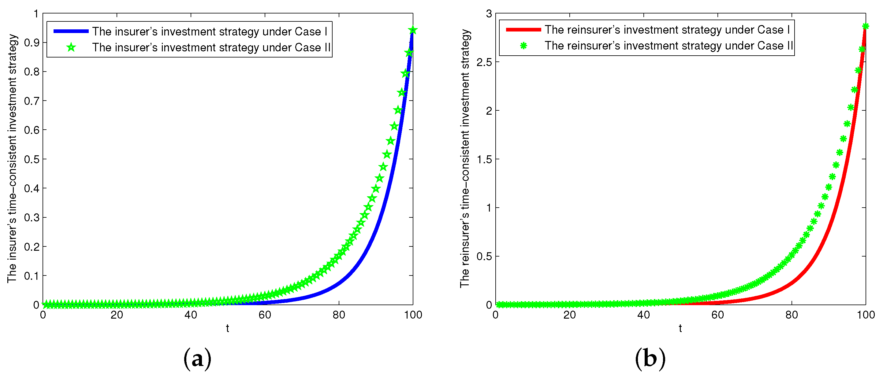
Figure 1 presents the evolution paths of the Nash equilibrium investment strategies when $x=1.2$ and the weight coefficient is $\alpha =0.2$. Figure 1a,b consider the effect of the intertemporal restrictions on the Nash equilibrium investment strategies (i.e., case I vs. case II). When $x=1.2$, the condition $\frac{x-s^2}{x^{T-t}-s^{2(T-t)}}\le \frac{1-s}{s^{T-t-1}(1-s^{T-t})}$ in Corollary 1 is satisfied. By comparing the investment strategies with and without intertemporal restrictions in Figure 1a,b, we can find that when the investment decision-making process considers intertemporal restrictions, the investors will reduce his/her investment position invested in the risk assessment (i.e., ${\widehat{u}}_t^1$ and ${\widehat{u}}_t^2$ will decrease) compared to the investment strategy without intertemporal restrictions. This phenomenon is consistent with the conclusions shown in Corollary 1. This means that intertemporal restrictions considerations will lead to an increase in the amount of investment in the riskless asset ($w_t^1-{\widehat{u}}_t^1$ and $w_t^2-{\widehat{u}}_t^2$), indicating that investors will adopt conservative strategies to reduce the investment risk.

Figure 2 depicts the evolution paths of the Nash equilibrium investment strategies when $x=1.01$ and the weight coefficient is $\alpha =0.2$. The effect of intertemporal restrictions on the Nash equilibrium investment strategies is considered in this simulation (i.e., cases I and II). When $x=1.01$, the condition $\frac{x-s^2}{x^{T-t}-s^{2(T-t)}}\ge \frac{1-s}{s^{T-t-1}(1-s^{T-t})}$ in Corollary 1 is satisfied. As shown in Figure 2, when the investment decision-making process considers intertemporal restrictions, investors will increase their exposure to risky assets compared to the investment strategy without intertemporal restrictions, which is consistent with the conclusions shown in Corollary 1. This means that the intertemporal restrictions will encourage investors to adopt radical strategies to increase their wealth. Compared with Figure 1 and Figure 2, we note that the effect of intertemporal restrictions on the Nash equilibrium investment strategies is related to the reduction speed of risk aversion parameters and the value of risk-free benefits.

In Figure 1 and Figure 2, we assume that the weight coefficient satisfies $\alpha <0.5$ (i.e., $\alpha =0.2$), which means that the interest of the reinsurer is relatively important in consideration of the common goal. Next, we want to test whether the above conclusions hold when the weight coefficient $\alpha >0.5$ (for example, $\alpha =0.8$ in Figure 3 and Figure 4).

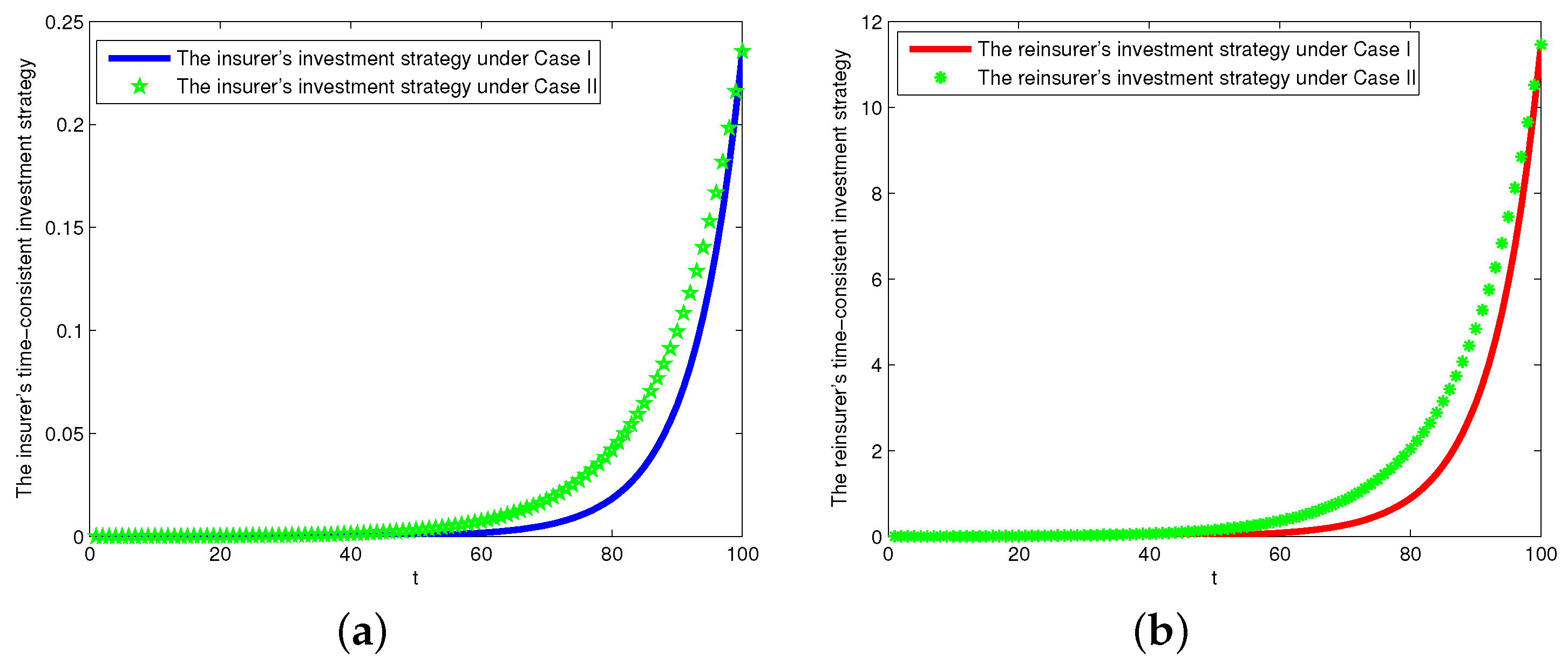
Comparing Figure 1 with Figure 3, Figure 2 with Figure 4, we find that the weight coefficient $\alpha$ can not change the effect of intertemporal constraints on investment strategies. In other words, whether the intertemporal restrictions will make the investment strategy more radical or more conservative depends only on the reduction speed of risk aversion parameters and the value of risk-free benefits, but not on the size of the weight parameter.

Moreover, in Figure 1, Figure 2, Figure 3 and Figure 4, we note that the Nash equilibrium investment strategies are increasing with respect to t. In other words, at the beginning of investment range, the insurer and the reinsurer are relatively conservative in order to avoid bankruptcy; the later, the more money they invest in risk assets. This phenomenon is because as time goes on, the insurer’s and reinsurer’s wealth keeps accumulating and their risk aversion coefficient gradually decreases, so they have enough ability and confidence to invest more funds in risky assets.

4.2. Simulations of the Nash Equilibrium Reinsurance Strategy

Next, we proceed to illustrate the evolution of the Nash equilibrium reinsurance strategy. On the basis of the parameters given above, we deduce the corresponding path of the Nash equilibrium reinsurance strategy. For details, see Figure 5, Figure 6, Figure 7 and Figure 8.

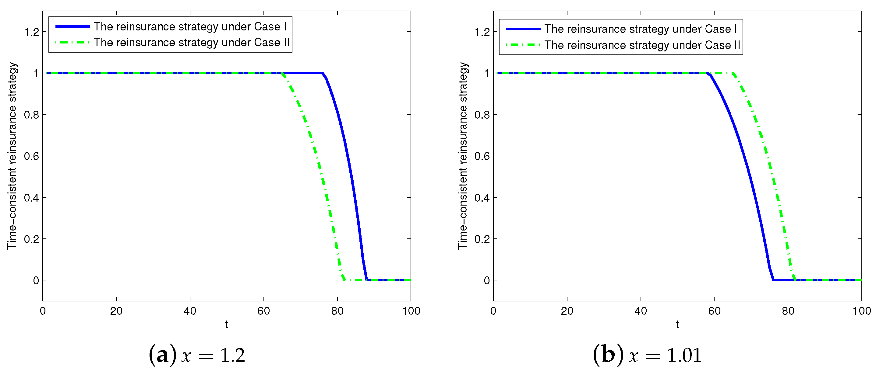
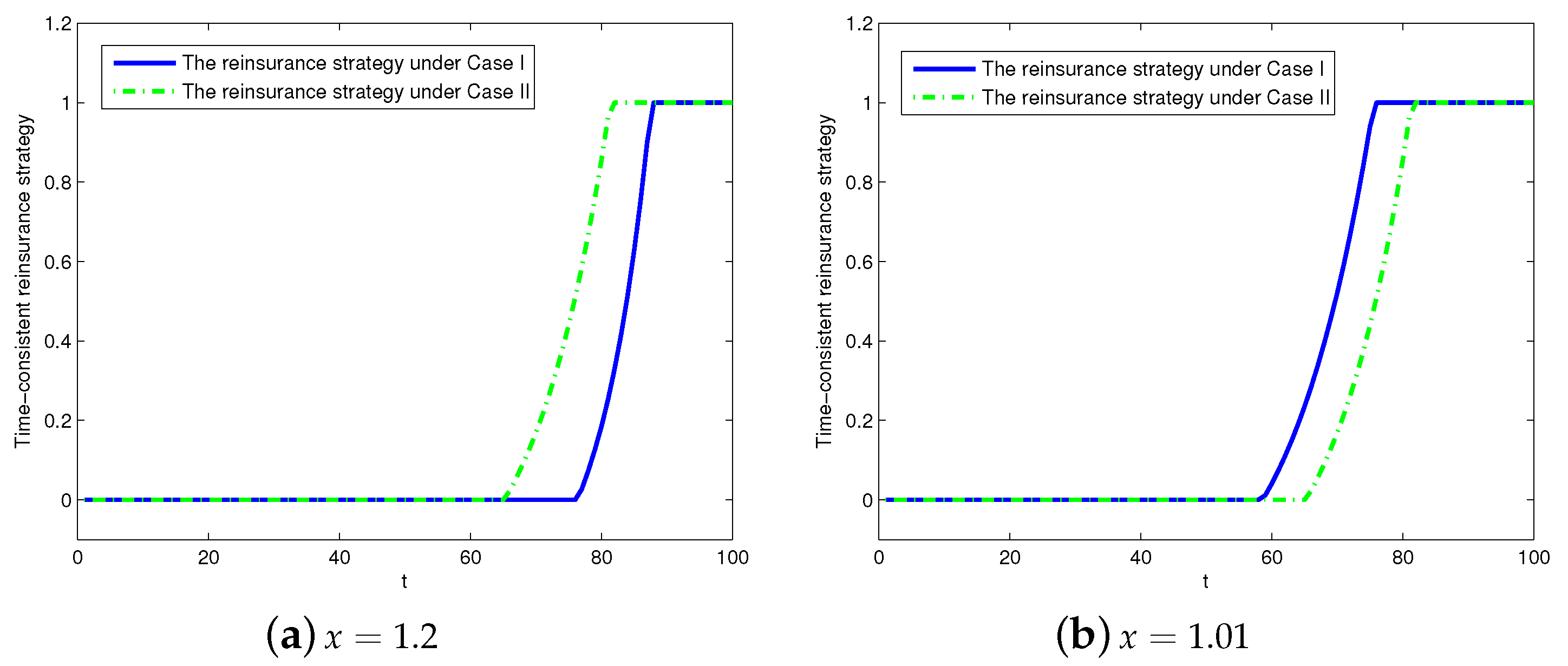
Under the expected value premium principle, Figure 5 shows the evolution of the Nash equilibrium reinsurance strategy when $\alpha <0.5$ (e.g., $\alpha =0.2$). As two different departments of the same large insurance company, the insurer and the reinsurer have a common interest goal, but their positions in the head office are different. $\alpha <0.5$ means that the interest of the reinsurer may be more concerned than that of the insurer. Therefore, the reinsurer may not be willing to bear the risk of claim, especially at the early stage. From Figure 5a, we can find that the reinsurer will not assume any claim risk in the previous investment periods (i.e., $q_t=1$ when $t\le 76$ in case I and $t\le 65$ in case II), and the reinsurer will only undertake the part or all of claim risk with the approach of the end of period (Note that ($1-q_t$) denotes the proportion of claim undertaken by reinsurer at time t, where $t=0,1,\cdots ,T-1$). A similar analysis can be obtained from Figure 5b.

In addition, in the case of $\alpha <0.5$, Figure 5a,b respectively describe the impacts of intertemporal restrictions on the Nash equilibrium reinsurance strategy when the reduction speed of risk aversion parameters takes different values. As shown in Figure 5a, we can find that the intertemporal restrictions can cause the reinsurer to be more concerned about its performance in the various intermediate periods, which will lead to longer time for the reinsurer not to bear the risk of claim (e.g., the reinsurance strategy of case I is $q_t=1$ when $t\le 76$, while that of case II is $q_t$ = 1 when $t\le 65$, this indicates that the reinsurer in the case I is less willing to take on the risk of claim compared to the reinsurer in the case II). When $x=1.2$, the condition $\frac{x-s^2}{x^{T-t}-s^{2(T-t)}}\le \frac{1-s}{s^{T-t-1}(1-s^{T-t})}$ in Corollary 3 is satisfied. That is, when the reinsurance strategy is between 0 and 1, the intertemporal restrictions reduce the underwriting ratio of the reinsurer, i.e., $(1-q_t)$ decreases. That is to say, intertemporal restrictions restrain the reinsurer’s enthusiasm to bear claim risk in this case.

From Figure 5b, we can find that intertemporal restrictions have a completely opposite effect on the Nash equilibrium reinsurance strategy. Intertemporal restrictions will make the reinsurer more confident about its own wealth level in this case and therefore more willing to take on claim risk as early as possible (e.g., the reinsurance strategy of case I is $q_t=1$ when $t\le 58$, while that of case II is $q_t$ = 1 when $t\le 65$, this indicates that the reinsurer in the case I is more willing to bear the claim risks compared to the reinsurer in the case II). When $x=1.01$, the condition $\frac{x-s^2}{x^{T-t}-s^{2(T-t)}}\ge \frac{1-s}{s^{T-t-1}(1-s^{T-t})}$ in Corollary 3 is satisfied. That is, when the reinsurance strategy is between 0 and 1, the intertemporal restrictions increase the underwriting ratio of the reinsurer, i.e., $(1-q_t)$ increases. In other words, intertemporal restrictions stimulate the reinsurer to bear the claim risk when $x=1.01$ and $\alpha <0.5$. In summary, when the reinsurer’s interest is more valued, the impact of intertemporal restrictions on Nash equilibrium reinsurance strategy is related to the values of reduction speed of risk aversion parameters and the value of risk-free benefits.

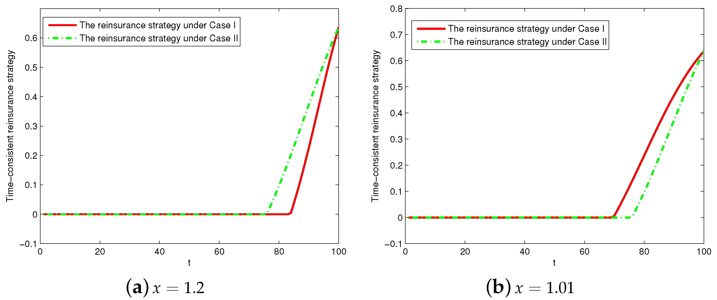
Figure 6 depicts the Nash equilibrium reinsurance strategy changes over time under expected value premium principle when the insurer’s interest is more valued (i.e., $\alpha >0.5$. As an example, we take $\alpha =0.8$ here). Similar to the analysis in Figure 5, from Figure 6, we find the insurer might want the reinsurer to assume more claim risks since the bankruptcy probability is higher in early stages of investment. With the insurer’s wealth accumulating, the insurer gradually improves the retention level $q_t$ of claim risk until it fully assumes all claim risk.

In addition, as shown in Figure 6a, we can find that, when the decision-making process does not consider intertemporal restrictions, the insurer will increase the retention level $q_t$ after $t=65$. When the decision-making process considers intertemporal restrictions, the insurer will increase the retention level $q_t$ after $t=76$. When the reinsurance strategy falls between 0 and 1, the intertemporal restrictions will reduce the insurer’s reservation level. In other words, the intertemporal restrictions will aggravate the insurer’s degree of risk aversion and make the insurer more reluctant to bear the claim risk prematurely when $x=1.2$ and $\alpha >0.5$. This is the opposite of the effect shown in Figure 6a. From Figure 6b, we can find that, when the decision-making process considers intertemporal restrictions, the insurer is more willing to assume a certain percentage or all of the claim risk as early as possible. Furthermore, the intertemporal restrictions will increase the insurer’s reservation level when the reinsurance strategy falls between 0 and 1. That is to say, intertemporal restrictions make the insurer more willing to take the claim risk when $x=1.01$ and $\alpha >0.5$. Combining Figure 6a,b, we find when the reinsurance premium is computed under the expected value premium principle, the effect of intertemporal restrictions on the Nash equilibrium reinsurance strategies depends not only on the reduction speed of risk aversion parameters and the value of risk-free benefits, but also on the weight parameter.

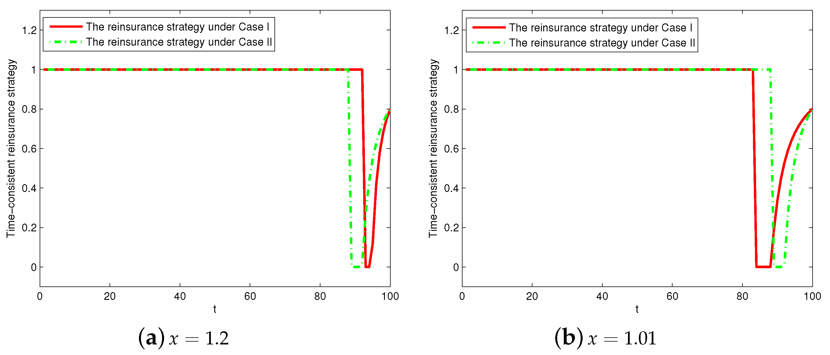
Figure 7 shows the Nash equilibrium reinsurance strategy changes over time under the variance value premium principle in the case of reinsurer’s interest is more valued (i.e., $\alpha <0.5$. For example, $\alpha =0.2$). From Figure 7, we can find that at the initial period, the reinsurer doesn’t want to take any the claim risk (i.e., $1-q_t=0$), and with the reinsurer accumulated to a certain degree of wealth, he/she has enough ability to take on all claim risks (i.e., $1-q_t=1$). As close to the end of investment, the insurer also has some ability to take the claim risk, then the retention level of the insurer (i.e., $q_t$) will be increased from 0 to a higher level.

Figure 7a,b depict the impacts of intertemporal restrictions on Nash equilibrium reinsurance strategy when x takes different values. As shown in Figure 7a, at the beginning of the period, the intertemporal restrictions will cause the reinsurer to pay more attention to his/her performance, which also lead to a longer time for the reinsurer to be unwilling to assume claim risk. At the end of the investment, the reinsurance strategy is between 0 and 1, and the intertemporal restrictions will increase the underwriting ratio of the reinsurer. From Figure 7b, at the beginning of the investment, the intertemporal restrictions make the reinsurer more confident about its level of wealth and therefore more willing to take on claim risk earlier. At the end of the investment, the reinsurance strategy is between 0 and 1, and the intertemporal restrictions will make the reinsurer reduce its underwriting proportion.

Figure 8 depicts the Nash equilibrium reinsurance strategies change over time under the variance value premium principle in the case of the insurer’s interest is more valued (i.e., $\alpha >0.5$. For example, $\alpha =0.8$). From Figure 8, we can find that the insurer will pass all claim risk to the reinsurer since the bankruptcy probability is higher in the early stages of investment. With the insurer’s wealth accumulating, the insurer has enough ability to bear claim risk; therefore, the insurer will gradually increase the retention level $q_t$. As shown in Figure 8a, the reinsurance strategy in case I will be shifted to the right by some units compared to that in case II. This illustrates the intertemporal restrictions will cause the insurer to pay more attention to its performance, which will lead to a longer time for the insurer to be unwilling to assume claim risk. When the reinsurance strategy is between 0 and 1, the intertemporal restrictions would encourage the insurer to reduce its reservation proportion. That is to say, the intertemporal restrictions can make the insurer more cautious about claim risk when $\alpha =0.8$ and $x=1.2$. From Figure 8b, we can find that the intertemporal restrictions make the insurer more confident about its level of wealth and more willing to take claims early (e.g., as shown in Figure 8a, the reinsurance strategy in case I will be shifted to the left by some units compared to that in case II). When the reinsurance strategy is between 0 and 1, the intertemporal restrictions would encourage the insurer to increase its reservation proportion. In other words, the intertemporal restrictions will make the insurer more willing to bear claim risks in this case.

5. Conclusions

In the paper, under the discrete-time framework, we construct a generalized multi-period mean-variance model to study the investment-reinsurance optimization problem of the reinsurer and the insurer, which can be regarded as two different departments of a general insurance company. The reinsurer and the insurer have a common interest goal to maximize the expectation of the weighted sum of their wealth processes and minimize corresponding variance. In addition, the intertemporal restrictions are considered in our model. By using the game method, we deduce the Nash equilibrium investment-reinsurance strategies for the generalized premium calculated principle, and derive the Nash equilibrium investment-reinsurance strategies under two special premium calculated principles (i.e., the expected value premium principle and the variance value premium principle). Furthermore, we theoretically analyze the effect of the intertemporal restrictions on Nash equilibrium strategies and perform corresponding numerical analyses to verify our theoretical results.

We find that the effect of the intertemporal restrictions on Nash equilibrium strategies is related to the setting of model parameters. (i) The effect of intertemporal restrictions on Nash equilibrium investment strategies depends on the reduction speed of risk aversion parameters and the value of risk-free benefits. (ii) When computing the reinsurance premium under the expected value premium principle, the effect of intertemporal restrictions on the Nash equilibrium reinsurance strategy depends not only on the reduction speed of risk aversion parameters and the value of risk-free benefits but also on the weight parameter. (iii) When computing the reinsurance premium under the variance value premium principle, the effect of intertemporal restrictions on the Nash equilibrium reinsurance strategy depends on a number of other factors, in addition to those mentioned above.

However, the research in this paper has some limitations. For example, this article studies equilibrium investment-reinsurance strategies under general or special reinsurance premium calculation rules but does not involve the pricing of reinsurance premiums. With the method in Chen and Shen [15], Chen and Shen [16] and Anthropelos and Boonen [38], how to find a reasonable reinsurance premium calculation formula to maximize the benefits of both the insurer and reinsurer in the discrete-time framework is an urgent problem to be studied. Furthermore, with reference to the methods of Bensoussan et al. [9], Pun and Wong [10], Pun et al. [11], and so on, the study of the game problem between two insurance companies in discrete-time framework is also a good expandable study direction of this paper in the future.