On Degenerate Truncated Special Polynomials

Abstract

The main aim of this paper is to introduce the degenerate truncated forms of multifarious special polynomials and numbers and is to investigate their various properties and relationships by using the series manipulation method and diverse special proof techniques. The degenerate truncated exponential polynomials are first considered and their several properties are given. Then the degenerate truncated Stirling polynomials of the second kind are defined and their elementary properties and relations are proved. Also, the degenerate truncated forms of the bivariate Fubini and Bell polynomials and numbers are introduced and various relations and formulas for these polynomials and numbers, which cover several summation formulas, addition identities, recurrence relationships, derivative property and correlations with the degenerate truncated Stirling polynomials of the second kind, are acquired. Thereafter, the truncated degenerate Bernoulli and Euler polynomials are considered and multifarious correlations and formulas including summation formulas, derivation rules and correlations with the degenerate truncated Stirling numbers of the second are derived. In addition, regarding applications, by introducing the degenerate truncated forms of the classical Bernstein polynomials, we obtain diverse correlations and formulas. Some interesting surface plots of these polynomials in the special cases are provided.

1. Introduction

Special functions possess a lot of importance in numerous fields of physics, mathematics, applied sciences, engineering and other related research areas including functional analysis, differential equations, quantum mechanics, mathematical analysis, mathematical physics, and so on [1,2,3,4,5,6,7,8,9,10,11,12,13,14,15,16,17,18,19,20,21,22,23,24,25,26,27,28,29,30,31,32,33,34,35,36] and see the references cited therein. For example; Riemann zeta function is closely related with the Bernoulli numbers and its zeros possess a connection with the distribution of prime numbers [12]. In particular, the family of special polynomials is one of the most useful and applicable family of special functions. Some of the most considerable polynomials in the theory of special polynomials are the Fubini polynomials (see [9,15,16,17,36]), the Bernoulli polynomials (see [2,5,6,7,11,13,29,31,32,33,34,35]), the Euler polynomials (see [2,5,6,7,11,27,29,31,32,33,34,35]), the Bernstein polynomials (see [1,20]) and the Bell polynomials (see [3,4,18,19,22,23,24,25]). Recently, the aforementioned polynomials and their several extensions have been densely studied and investigated by diverse mathematicians and physicists [1,2,3,4,5,6,7,8,9,10,11,12,13,14,15,16,17,18,19,20,21,22,23,24,25,26,27,28,29,30,31,32,33,34,35,36] and see also each of the references cited therein.

Throughout this paper, the familiar symbols $\mathbb{C}$, $\mathbb{R}$, $\mathbb{Z}$, $\mathbb{N}$ and ${\mathbb{N}}_0$ are referred to the set of all complex numbers, the set of all real numbers, the set of all integers, the set of all natural numbers and the set of all non-negative integers, respectively.

The truncated exponential polynomials $e_n\left(x\right)$ are the first $\left(n+1\right)$ terms of the Mac Laurin series for $e^x$ ([8]), i.e.,

$$e_n\left(x\right)=\sum _{k=0}^n\frac{x^k}{k!}.$$

(1)

This polynomial has the following integral representation:

$$e_n\left(x\right)=\sum _{k=0}^n\frac{x^k}{k!}\frac{\left(n-k\right)!}{\left(n-k\right)!}=\frac{1}{n!}{\int }_0^{\infty }{e}^{\beta }{\left(x+\beta \right)}^{n}d\beta .$$

(2)

The classical generating function of the truncated exponential polynomials is as follows ([8])

$$\sum _{n=0}^{\infty }{e}_n\left(x\right)t^n=\frac{e^{tx}}{1-t}.$$

(3)

By means of the aforesaid generating function, one can easily get the following derivative relations:

$$e_{n+1}=\left[1+\frac{x}{n+1}\left(1-\frac{d}{dx}\right)\right]e_n\left(x\right)$$

(4)

and

$$e_{n-1}\left(x\right)=\frac{d}{dx}{e}_n\left(x\right).$$

(5)

For more detailed information about the truncated exponential polynomials, see [8] and the references cited therein.

The traditional Pochhammer symbol ${\left(x\right)}_n$ (sometimes called the descending factorial, falling sequential product, falling factorial, or lower factorial) is defined by (see [2,3,5,10,11,17,20,21,22,23,25,26,34])

$${\left(x\right)}_n=\left\{\begin{array}{cc}x(x-1)(x-2)\cdots (x-(n-1\left)\right),\hfill & n\in \mathbb{N}\hfill \\ 1\hfill & n=0.\hfill \end{array}\right.$$

(6)

The $\lambda$-extension of the usual Pochhammer symbol ${\left(x\right)}_{n,\lambda }$ is given by (see [5,10,11,17,20,21,22,23,25,26])

$${\left(x\right)}_{n,\lambda }=\left\{\begin{array}{cc}x(x-\lambda )(x-2\lambda )\cdots (x-(n-1\left)\lambda \right),\hfill & n\in \mathbb{N}\hfill \\ 1\hfill & n=0.\hfill \end{array}\right.$$

(7)

Please note that ${\left(x\right)}_{n,1}:={\left(x\right)}_n$.

The ${\mathsf{\Delta }}_{\lambda }$ difference operator of a function is defined by (see [11])

$${\mathsf{\Delta }}_{\lambda }f\left(x\right)={\displaystyle \frac{1}{\lambda }}(f(x+\lambda )-f\left(x\right)),\alpha \ne 0.$$

(8)

The following difference rule holds true ([11]):

$${\mathsf{\Delta }}_{\lambda }^k{\left(x\right)}_{n,\lambda }={\displaystyle \frac{n!}{(n-k)!}}{\left(x\right)}_{n-k,\lambda },0\le k\le n,$$

(9)

where the notation ${\mathsf{\Delta }}_{\lambda }^k$ denotes the k times applying the ${\mathsf{\Delta }}_{\lambda }$ difference operators.

Let $\lambda \in \mathbb{R}/\left\{0\right\}$. The degenerate exponential function $e_{\lambda }^x\left(t\right)$ is defined by ([5,10,11,14,17,20,21,22,23,25,26])

$$e_{\lambda }^x\left(t\right)={\left(1+\lambda t\right)}^{\frac{x}{\lambda }}\mathrm{and}{e}_{\lambda }^1\left(t\right)=e_{\lambda }\left(t\right).$$

(10)

It is readily seen that ${lim}_{\lambda \to 0}{e}_{\lambda }^x\left(t\right)=e^{xt}$. From (10), we obtain the following relation

$$e_{\lambda }^x\left(t\right)=\sum _{n=0}^{\infty }{\left(x\right)}_{n,\lambda }\frac{t^n}{n!},$$

(11)

which satisfies the following difference rule

$${\mathsf{\Delta }}_{\lambda }{e}_{\lambda }^x\left(t\right)=t{e}_{\lambda }^x\left(t\right).$$

(12)

By Equation (11), we can write

$$e_{\lambda }\left(t\right)=\sum _{n=0}^{\infty }{\left(1\right)}_{n,\lambda }\frac{t^n}{n!}=1+{\left(1\right)}_{1,\lambda }\frac{t}{1!}+{\left(1\right)}_{2,\lambda }\frac{t^2}{2!}+{\left(1\right)}_{3,\lambda }\frac{t^3}{3!}+\cdots .$$

While the truncated exponential polynomials $e_n\left(x\right)$ (1) are the first $\left(n+1\right)$ terms of the Mac Laurin series for usual exponential function $e^x$, the degenerate truncated exponential polynomials are introduced as the first $\left(n+1\right)$ terms of the Mac Laurin series expansion of the degenerate exponential function $e_{\lambda }\left(t\right)$ in (11) will be given in the next section.

The generating function is a key tool for a family of special polynomials if they have to derive their properties and relations. It is also used in other fields, for example, a study of false positive/negative effects on network robustness [37] and in statistics as moment generating function [10].

Carlitz [5] introduced and studied the degenerate Bernoulli polynomials by means of the degenerate exponential functions as follows:

$$\sum _{n=0}^{\infty }{B}_{n,\lambda }\left(x\right)\frac{t^n}{n!}=\frac{t}{e_{\lambda }\left(t\right)-1}{e}_{\lambda }^x\left(t\right).$$

Then Howard [14] provided several explicit formulas for the degenerate Bernoulli polynomials and gave a new proof of the degenerate Staudt-Clausen theorem. In the recent years, the degenerate forms for the specials polynomials have been heavily considered and developed by many mathematicians [5,10,11,14,17,20,21,22,23,25,26] and see also each of the references cited therein. Duran et al. [10] considered three extensions of the Stirling polynomials of the second kind by means of the degenerate exponential functions and then showed that these polynomials appear in the expressions of the probability distributions of proper random variables such as degenerate Poisson distribution, degenerate zero-truncated Poisson distribution and degenerate r-truncated Poisson distribution. Duran et al. [11] introduced the Gould–Hopper-based fully degenerate poly-Bernoulli polynomials with a q-parameter and developed their properties and relations. Kim et al. [17] defined a new class of degenerate Fubini numbers and polynomials and investigated diverse properties of these polynomials and numbers. Kim et al. [20] introduced the degenerate Bernstein polynomials and acquired their exponential generating function, recurrence relations, symmetric identities, and some connected formulas with generalized falling factorial polynomials, higher-order degenerate Bernoulli polynomials and degenerate Stirling numbers of the second kind. Kim et al. [21] the degenerate $\lambda$-Stirling polynomials of the second kind and provided some applications for these polynomials. Kim et al. [22] defined the degenerate Bell numbers and polynomials and examined various novel relations and formulas. Kim et al. [23] studied the degenerate r-Stirling numbers of the second kind and the degenerate r-Bell polynomials investigated several properties, recurrence relations and formulas by means of umbral calculus. Kim et al. [25] considered the partially degenerate Bell polynomials numbers and developed their properties and identities. Kim et al. [26] defined the degenerate Stirling polynomials of the second kind and gave some new identities for these polynomials.

In the family of special polynomials, in the recent years, the truncated forms for polynomials have been worked and investigated by various mathematicians [8,9,13,27,33] and see also the references cited therein. Dattoli et al. [8] introduced the higher-order truncated polynomials which plays a role of crucial importance in the evaluation of integrals involving products of special functions and discussed them within the more general context of the Appell family and the Laguerre family. Duran et al. [9] considered the two-variable truncated Fubini polynomials and numbers and then investigated multifarious relations and formulas including summation formulas, recurrence relations, derivative property and correlations with the truncated Stirling numbers of the second kind, Apostol-type Stirling numbers of the second kind, the truncated Bernoulli polynomials and truncated Euler polynomials. Hassen et al. [13] defined the truncated Bernoulli polynomials and derived several properties. Komatsu et al. [27] considered the truncated Euler polynomials and presented their some properties and relations with the truncated Bernoulli polynomials. Srivastava et al. [33] examined the truncated-exponential-based Apostol-type polynomials and derived their various properties covering some implicit summation formulas and symmetric identities.

The rest of this paper is structured as follows: Section 2 provides the definition of the degenerate truncated exponential polynomials and then proves their properties. In Section 3, the degenerate truncated Stirling polynomials of the second kind are introduced and their elementary properties and relations are examined properly. The Section 4 deals with the degenerate forms of the bivariate truncated Fubini polynomials and numbers and then investigates several relations and formulas for these polynomials and numbers, which covers several summation formulas, addition identities, recurrence relationships, derivative property and correlations with the degenerate truncated Stirling polynomials of the second kind. The truncated degenerate Bernoulli and Euler polynomials are introduced and multifarious correlations and formulas including summation formulas, derivation rules and correlations with the degenerate truncated Stirling numbers of the second kind are derived in the Section 5. Section 6 includes the definition of the degenerate truncated forms of the bivariate Bell polynomials and numbers and also diverse identities and correlations, which includes addition formulas, summation formulas, recurrence relationships, difference operator property and derivative rules are acquired. Section 7 first supplies the degenerate truncated forms of the classical Bernstein polynomials and then investigates diverse correlations and formulas including several polynomials such as the degenerate truncated Bernstein polynomials, the bivariate $Detr$-Fubini polynomials, the bivariate $Detr$-Bell polynomials, the $Detr$-Bernoulli polynomials, the $Detr$-Stirling polynomials of the second kind and the $Detr$-Euler polynomials. The last section of this paper analyzes the results obtained in this paper.

2. The Truncated Degenerate Exponential Polynomials

In this section, we consider the degenerate truncated exponential polynomials and then investigate their properties.

We consider the degenerate form of the truncated exponential polynomials, therefore we give the following definition.

Definition 1.

The degenerate truncated exponential polynomials are introduced as the first $\left(n+1\right)$ terms of the Taylor series expansion of $e_{\lambda }\left(t\right)$ in (11) at $t=0$:

$$e_{n,\lambda }\left(t\right)=\sum _{k=0}^n{\left(1\right)}_{k,\lambda }\frac{t^k}{k!}.$$

(13)

We choose to call the $Detr$-exponential polynomials as well as the degenerate truncated exponential polynomials.

We now examine a special case of the aforementioned polynomials as follows.

Remark 1.

When $\lambda \to 0$, the $Detr$-exponential polynomials $e_{n,\lambda }\left(t\right)$ (13) reduces to the truncated exponential polynomials $e_n\left(t\right)$ in (1).

The classical exponential generating function of the $Detr$-exponential polynomials are given by the following proposition.

Proposition 1.

For $\left|z\right|<1$, we have

$$\sum _{n=0}^{\infty }{e}_{n,\lambda }\left(t\right)z^n=\frac{e_{\lambda }\left(zt\right)}{1-z}.$$

(14)

Proof. 

To find the generating function of the $Detr$-exponential polynomials, for $\left|z\right|<1$, we consider

$$\begin{array}{cc}\hfill \sum _{n=0}^{\infty }{e}_{n,\lambda }\left(t\right)z^n& =\sum _{n=0}^{\infty }\sum _{k=0}^n{\left(1\right)}_{k,\lambda }\frac{t^k}{k!}{z}^n\hfill \\ & =\sum _{n=0}^{\infty }{\left(1\right)}_{n,\lambda }\frac{{\left(zt\right)}^n}{n!}\sum _{k=0}^n{z}^n\hfill \\ & =\frac{e_{\lambda }\left(zt\right)}{1-z},\hfill \end{array}$$

which implies the assertion (14). □

We now give the following proposition.

Proposition 2.

The following difference operator rule holds true:

$${\mathsf{\Delta }}_{\lambda ,}{e}_{n,\lambda }\left(t\right)=t{e}_{n-1,\lambda }\left(t\right).$$

(15)

Proof. 

By means of (14), we observe

$$\begin{array}{ccc}\hfill \sum _{n=0}^{\infty }{\mathsf{\Delta }}_{\lambda }{e}_{n,\lambda }\left(t\right)z^n& =& \frac{1}{1-z}{\mathsf{\Delta }}_{\lambda }{e}_{\lambda }\left(zt\right)\hfill \\ & =& \frac{1}{1-z}\sum _{n=0}^{\infty }{\mathsf{\Delta }}_{\lambda }{\left(1\right)}_{n,\lambda }\frac{{\left(zt\right)}^n}{n!}\hfill \\ & =& \frac{1}{1-z}\sum _{n=1}^{\infty }{\left(1\right)}_{n-1,\lambda }\frac{{\left(zt\right)}^n}{\left(n-1\right)!}\hfill \\ & =& \frac{zt}{1-z}\sum _{n=0}^{\infty }{\left(1\right)}_{n,\lambda }\frac{{\left(zt\right)}^n}{n!}\hfill \\ & =& \sum _{n=0}^{\infty }t{e}_{n,\lambda }\left(t\right)z^{n+1},\hfill \end{array}$$

which gives the claimed result (15) by comparing the coefficients of the first and the last series with respect to z. □

We provide the following recurrence formula.

Proposition 3.

The following recurrence relation

$$e_{n+1,\lambda }\left(t\right)=\left(n+1\right)\sum _{k=0}^n\left({\left(1\right)}_{k+1,\lambda }\frac{t^{k+1}}{k!}+e_{k,\lambda }\left(t\right)\right)$$

(16)

is valid for $n\in {\mathbb{N}}_0$.

Proof. 

By Equation (14), we observe that

$$\begin{array}{c}\sum _{n=0}^{\infty }{e}_{n,\lambda }\left(t\right)\frac{d}{dz}{z}^n=\frac{d}{dz}\left(\frac{e_{\lambda }\left(zt\right)}{1-z}\right)\\ =\frac{\left(1-z\right)\frac{d}{dz}{e}_{\lambda }\left(zt\right)+e_{\lambda }\left(zt\right)}{{\left(1-z\right)}^2}\\ =\frac{1}{{\left(1-z\right)}^2}\left(\left(1-z\right)\sum _{n=0}^{\infty }{\left(1\right)}_{n,\lambda }{t}^n\frac{\frac{d}{dt}{z}^n}{n!}+e_{\lambda }\left(zt\right)\right)\\ =\sum _{n=0}^{\infty }{z}^n\sum _{n=0}^{\infty }{\left(1\right)}_{n+1,\lambda }{t}^{n+1}\frac{z^n}{n!}+\sum _{n=0}^{\infty }{z}^n\sum _{n=0}^{\infty }{e}_{n,\lambda }\left(t\right)z^n\\ =\sum _{n=0}^{\infty }\sum _{k=0}^n{\left(1\right)}_{k+1,\lambda }\frac{t^{k+1}}{k!}{z}^n+\sum _{n=0}^{\infty }\sum _{k=0}^n{e}_{k,\lambda }\left(t\right)z^n,\end{array}$$

which gives

$$e_{n+1,\lambda }\left(t\right)=\sum _{k=0}^n{\left(1\right)}_{k+1,\lambda }\frac{t^{k+1}}{k!}+\sum _{k=0}^n{e}_{k,\lambda }\left(t\right),$$

which means the asserted result (16). □

3. Degenerate Truncated Stirling Polynomials of the Second Kind

In this section, we introduce the degenerate truncated Stirling polynomials of the second kind and analyze their elementary properties and relations.

The Stirling polynomials $S_2\left(n,k:x\right)$ and numbers $S_2\left(n,k\right)$ of the second kind are given by the following exponential generating functions ([9,10,11,18,21,23,24,26,34]):

$$\sum _{n=0}^{\infty }{S}_2\left(n,k:x\right)\frac{t^n}{n!}=\frac{{\left(e^t-1\right)}^k}{k!}{e}^{tx}\mathrm{and}\sum _{n=0}^{\infty }{S}_2\left(n,k\right)\frac{t^n}{n!}=\frac{{\left(e^t-1\right)}^k}{k!}.$$

(17)

In combinatorics, Stirling number of second kind $S_2\left(n,k\right)$ counts number of ways in which n distinguishable objects can be partitioned into k indistinguishable subsets when each subset must contain at least one object. The Stirling numbers of the second kind can also be derived by the following recurrence relation for a fixed non-negative integer $\zeta$([9,10,11,18,21,23,24,26,34]):

$$x^{\zeta }=\sum _{\mu =0}^{\zeta }{S}_2\left(\zeta ,\mu \right){\left(x\right)}_{\mu },$$

(18)

where the notation ${\left(x\right)}_{\mu }$ is mentioned in (6).

Let $k\in {\mathbb{N}}_0$ and $\alpha \in \mathbb{C}$. The Apostol-type Stirling polynomials $S_2^{\alpha }\left(n,k:x\right)$ and numbers $S_2^{\alpha }\left(n,k\right)$ of the second kind is defined as follows ([28]):

$$\sum _{n=0}^{\infty }{S}_2^{\alpha }\left(n,k:x\right)\frac{t^n}{n!}=\frac{{\left(\alpha e^t-1\right)}^k}{k!}{e}^{tx}\mathrm{and}\sum _{n=0}^{\infty }{S}_2^{\alpha }\left(n,k\right)\frac{t^n}{n!}=\frac{{\left(\alpha e^t-1\right)}^k}{k!}.$$

(19)

Here is the definition of the degenerate truncated Apostol-type Stirling polynomials of the second kind which we choose to call the Apostol-type $Detr$-Stirling polynomials of the second kind as follows.

Definition 2.

Let x be an independent variable. The degenerate truncated Apostol-type Stirling polynomials and numbers of the second kind are introduced by the following generating functions:

$$\sum _{n=0}^{\infty }{S}_{2,m;\lambda }^{\alpha }\left(n,k:x\right)\frac{t^n}{n!}=\frac{{\left(\alpha e_{\lambda }\left(t\right)-1-e_{m-1,\lambda }\left(t\right)\right)}^k}{k!}{e}_{\lambda }^x\left(t\right)$$

(20)

and

$$\sum _{n=0}^{\infty }{S}_{2,m;\lambda }^{\alpha }\left(n,k\right)\frac{t^n}{n!}=\frac{{\left(\alpha e_{\lambda }\left(t\right)-1-e_{m-1,\lambda }\left(t\right)\right)}^k}{k!}$$

(21)

Diverse special circumstances of $S_{2,m;\lambda }^{\alpha }\left(n,k:x\right)$ and $S_{2,m;\lambda }^{\alpha }\left(n,k\right)$ are discussed below:

Remark 2.

In the case $\alpha =0$ in (20), we attain the $Detr$-Stirling polynomials and numbers of the second kind $S_{2,m;\lambda }\left(n,k\right)$ and $S_{2,m;\lambda }\left(n,k\right)$, which are also new generalizations of the usual Stirling polynomials and numbers of the second kind in (17), as follows:

$$\sum _{n=0}^{\infty }{S}_{2,m;\lambda }\left(n,k:x\right)\frac{t^n}{n!}=\frac{{\left(e_{\lambda }\left(t\right)-1-e_{m-1,\lambda }\left(t\right)\right)}^k}{k!}{e}_{\lambda }^x\left(t\right)$$

(22)

and

$$\sum _{n=0}^{\infty }{S}_{2,m;\lambda }\left(n,k\right)\frac{t^n}{n!}=\frac{{\left(e_{\lambda }\left(t\right)-1-e_{m-1,\lambda }\left(t\right)\right)}^k}{k!}$$

(23)

Remark 3.

When λ approaches to zero, the Apostol-type $Detr$-Stirling polynomials of the second kind $S_{2,m;\lambda }^{\alpha }\left(n,k:x\right)$ become the truncated Apostol-type Stirling polynomials of the second kind $S_{2,m}^{\alpha }\left(n,k:x\right)$ given by the following series expansion ([10,21]):

$$\sum _{n=0}^{\infty }{S}_{2,m}^{\alpha }\left(n,k:x\right)\frac{t^n}{n!}=\frac{{\left(\alpha e^t-1-{\sum }_{j=0}^{m-1}\frac{t^j}{j!}\right)}^k}{k!}{e}^{xt}.$$

(24)

Remark 4.

Substituting $\lambda \to m=0$ in (20), we get the degenerate Apostol-type Stirling polynomials of the second kind $S_{2,\lambda }\left(n,k\right)$ defined by ([10,21,23]):

$$\sum _{n=0}^{\infty }{S}_{2,\lambda }^{\alpha }\left(n,k:x\right)\frac{t^n}{n!}=\frac{{\left(\alpha e_{\lambda }\left(t\right)-1\right)}^k}{k!}{e}_{\lambda }^x\left(t\right).$$

(25)

Remark 5.

Letting $\lambda \to m=\alpha =0$ in (20), we obtain the degenerate Stirling polynomials of the second kind $S_{2,\lambda }\left(n,k\right)$ provided by ([10,21,23]):

$$\sum _{n=0}^{\infty }{S}_{2,\lambda }\left(n,k:x\right)\frac{t^n}{n!}=\frac{{\left(e_{\lambda }\left(t\right)-1\right)}^k}{k!}{e}_{\lambda }^x\left(t\right).$$

(26)

Remark 6.

Upon setting $\lambda \to m=\alpha =0$ in (20), the truncated Stirling numbers of the second kind $S_{2,m}\left(n,k\right)$ reduce to the classical Stirling numbers of the second kind by (17).

We now ready to derive some properties of the $S_{2,m;\lambda }^{\alpha }\left(n,k:x\right)$. By means of (20) and (21), we observe that

$$\begin{array}{ccc}\hfill \sum _{n=0}^{\infty }{S}_{2,m;\lambda }^{\alpha }\left(n,k:x\right)\frac{t^n}{n!}& =& \frac{{\left(\alpha e_{\lambda }\left(t\right)-1-e_{m-1,\lambda }\left(t\right)\right)}^k}{k!}{e}_{\lambda }^x\left(t\right)\hfill \\ & =& \sum _{n=0}^{\infty }{S}_{2,m;\lambda }^{\alpha }\left(n,k\right)\frac{t^n}{n!}\sum _{n=0}^{\infty }{\left(x\right)}_{n,\lambda }\frac{t^n}{n!}\hfill \\ & =& \sum _{n=0}^{\infty }\sum _{l=0}^n\left(\genfrac{}{}{0pt}{}{n}{l}\right)S_{2,m;\lambda }^{\alpha }\left(l,k\right){\left(x\right)}_{n-l,\lambda }\frac{t^n}{n!}.\hfill \end{array}$$

Henceforth, we state the following relation.

Proposition 4.

The following relation holds true:

$$S_{2,m;\lambda }^{\alpha }\left(n,k:x\right)=\sum _{l=0}^n\left(\genfrac{}{}{0pt}{}{n}{l}\right)S_{2,m;\lambda }^{\alpha }\left(l,k\right){\left(x\right)}_{n-l,\lambda }.$$

By Equation (20), we get

$$\begin{array}{ccc}\hfill \sum _{n=0}^{\infty }{S}_{2,m;\lambda }^{\alpha }\left(n,k:x+y\right)\frac{t^n}{n!}& =& \frac{{\left(\alpha e_{\lambda }\left(t\right)-1-e_{m-1,\lambda }\left(t\right)\right)}^k}{k!}{e}_{\lambda }^x\left(t\right)e_{\lambda }^y\left(t\right)\hfill \\ & =& \sum _{n=0}^{\infty }{S}_{2,m;\lambda }^{\alpha }\left(n,k:x\right)\frac{t^n}{n!}\sum _{n=0}^{\infty }{\left(y\right)}_{n,\lambda }\frac{t^n}{n!}\hfill \\ & =& \sum _{n=0}^{\infty }\sum _{u=0}^n\left(\genfrac{}{}{0pt}{}{n}{u}\right)S_{2,m;\lambda }^{\alpha }\left(u,k:x\right){\left(y\right)}_{n-u,\lambda }\frac{t^n}{n!},\hfill \end{array}$$

which yields the following result.

Proposition 5.

The following summation formula holds true:

$$S_{2,m;\lambda }^{\alpha }\left(n,k:x+y\right)=\sum _{u=0}^n\left(\genfrac{}{}{0pt}{}{n}{u}\right)S_{2,m;\lambda }^{\alpha }\left(u,k:x\right){\left(y\right)}_{n-u,\lambda }.$$

The Apostol-type $Detr$-Stirling polynomials of the second kind satisfy the following correlation.

Proposition 6.

The following relation

$$S_{2,m}\left(n,k+l\right)=\frac{r!k!}{\left(k+r\right)!}\sum _{u=0}^n\left(\genfrac{}{}{0pt}{}{n}{u}\right)S_{2,m;\lambda }^{\alpha }\left(u,k:x\right)S_{2,m;\lambda }^{\alpha }\left(n-u,r:y\right)$$

(27)

is valid for non-negative integers m and n.

Proof. 

In view of Equations (17) and (20), we have

$$\begin{array}{c}\sum _{n=0}^{\infty }{S}_{2,m;\lambda }^{\alpha }\left(n,k+r:x+y\right)\frac{t^n}{n!}=\frac{{\left(\alpha e_{\lambda }\left(t\right)-1-e_{m-1,\lambda }\left(t\right)\right)}^{k+r}}{\left(k+r\right)!}{e}_{\lambda }^{x+y}\left(t\right)\\ =\frac{r!k!}{\left(k+r\right)!}\frac{{\left(\alpha e_{\lambda }\left(t\right)-1-e_{m-1,\lambda }\left(t\right)\right)}^k}{k!}{e}_{\lambda }^x\left(t\right)\frac{{\left(\alpha e_{\lambda }\left(t\right)-1-e_{m-1,\lambda }\left(t\right)\right)}^r}{r!}{e}_{\lambda }^y\left(t\right)\\ =\frac{r!k!}{\left(k+r\right)!}\sum _{n=0}^{\infty }{S}_{2,m;\lambda }^{\alpha }\left(n,k:x\right)\frac{t^n}{n!}\sum _{n=0}^{\infty }{S}_{2,m;\lambda }^{\alpha }\left(n,r:y\right)\frac{t^n}{n!}\\ =\frac{r!k!}{\left(k+r\right)!}\sum _{n=0}^{\infty }\sum _{u=0}^n\left(\genfrac{}{}{0pt}{}{n}{u}\right)S_{2,m;\lambda }^{\alpha }\left(u,k:x\right)S_{2,m;\lambda }^{\alpha }\left(n-u,r:y\right)\frac{t^n}{n!},\end{array}$$

which means the asserted result (27). □

We now provide the following relationship.

Proposition 7.

The following relation

$$S_{2,1;\lambda }\left(n,k:x\right)=2^k{S}_{2,\lambda }^{1/2}\left(n,k:x\right)$$

(28)

holds true for non-negative integers m and n.

Proof. 

In view of (22) and (25), we have

$$\begin{array}{ccc}\hfill \sum _{n=0}^{\infty }{S}_{2,1;\lambda }\left(n,k:x\right)\frac{t^n}{n!}& =& \frac{{\left(e_{\lambda }\left(t\right)-1-1\right)}^k}{k!}{e}_{\lambda }^x\left(t\right)\hfill \\ & =& \frac{2^k{\left(\frac{1}{2}{e}_{\lambda }\left(t\right)-1\right)}^k}{k!}{e}_{\lambda }^x\left(t\right)\hfill \\ & =& 2^k\sum _{n=0}^{\infty }{S}_{2,\lambda }^{1/2}\left(n,k:x\right)\frac{t^n}{n!},\hfill \end{array}$$

which presents the desired result (28). □

We give the following proposition below.

Proposition 8.

The following series representation

$$S_{2,m+1;\lambda }^{\alpha }\left(n,k:x\right)=\sum _{l=0}^k\frac{n!{\left(1\right)}_{m,\lambda }^l}{{\left(m!\right)}^l\left(n-ml\right)!l!}{S}_{2,m;\lambda }^{\alpha }\left(n-ml,k-l:x\right)$$

(29)

is valid for non-negative integers m and n.

Proof. 

From Equation (20), we see that

$$\begin{array}{ccc}\hfill \sum _{n=0}^{\infty }{S}_{2,m+1;\lambda }^{\alpha }\left(n,k:x\right)\frac{t^n}{n!}& =& \frac{{\left(\alpha e_{\lambda }\left(t\right)-1-e_{m,\lambda }\left(t\right)\right)}^k}{k!}{e}_{\lambda }^x\left(t\right)\hfill \\ & =& \frac{{\left(\alpha e_{\lambda }\left(t\right)-1-e_{m-1,\lambda }\left(t\right)-{\left(1\right)}_{m,\lambda }\frac{t^m}{m!}\right)}^k}{k!}{e}_{\lambda }^x\left(t\right)\hfill \\ & =& \frac{e_{\lambda }^x\left(t\right)}{k!}\sum _{l=0}^k\left(\genfrac{}{}{0pt}{}{k}{l}\right){\left(\alpha e_{\lambda }\left(t\right)-1-e_{m-1,\lambda }\left(t\right)\right)}^{k-l}{\left(1\right)}_{m,\lambda }^l\frac{t^{ml}}{{\left(m!\right)}^l}\hfill \\ & =& \sum _{l=0}^k\frac{{\left(1\right)}_{m,\lambda }^l}{l!}\frac{t^{ml}}{{\left(m!\right)}^l}\frac{{\left(\alpha e_{\lambda }\left(t\right)-1-e_{m-1,\lambda }\left(t\right)\right)}^{k-l}}{\left(k-l\right)!}{e}_{\lambda }^x\left(t\right)\hfill \\ & =& \sum _{l=0}^k\frac{{\left(1\right)}_{m,\lambda }^l}{l!}\frac{t^{ml}}{{\left(m!\right)}^l}\sum _{n=0}^{\infty }{S}_{2,m;\lambda }^{\alpha }\left(n,k-l:x\right)\frac{t^n}{n!}\hfill \\ & =& \sum _{n=0}^{\infty }\sum _{l=0}^k\frac{{\left(1\right)}_{m,\lambda }^l}{l!}\frac{S_{2,m;\lambda }^{\alpha }\left(n,k-l:x\right)}{{\left(m!\right)}^l}\frac{t^{n+ml}}{n!},\hfill \end{array}$$

which implies the asserted result (29). □

4. The Truncated Degenerate Fubini Polynomials

In this section, we perform to introduce and analyze the degenerate forms of the bivariate truncated Fubini polynomials and numbers. We then investigate many relations and formulas for these polynomials and numbers, which covers several summation formulas, addition identities, recurrence relationships and derivative property. We also give some formulas associated with the Apostol-type $Detr$-Stirling polynomials of the second kind and the $Detr$-Stirling polynomials of the second kind.

We first remember the usual two variables Fubini polynomials by the following generating function ([9,15,16,36]):

$$\sum _{n=0}^{\infty }{F}_n\left(x,y\right)\frac{t^n}{n!}=\frac{e^{xt}}{1-y\left(e^t-1\right)}.$$

(30)

When $x=0$ in (30), the two variables Fubini polynomials $F_n\left(x,y\right)$ reduce to the usual Fubini polynomials given by ([9,15,16,17,36]):

$$\sum _{n=0}^{\infty }{F}_n\left(y\right)\frac{t^n}{n!}=\frac{1}{1-y\left(e^t-1\right)}.$$

(31)

For $n\in {\mathbb{N}}_0$, it is not difficult to investigate the following correlations ([9,16,17,36]):

$$F_n\left(y\right)=\sum _{\mu =0}^n{S}_2\left(n,\mu \right)\mu !y^{\mu }.$$

(32)

Substituting y by 1 in (31), we have the familiar Fubini numbers $F_n\left(1\right):=F_n$ ([9,16,17,36]) below:

$$\sum _{n=0}^{\infty }{F}_n\frac{t^n}{n!}=\frac{1}{2-e^t}.$$

(33)

For non-negative integer m, the bivariate truncated Fubini polynomials are defined via the following exponential generating function [9]:

$$\sum _{n=0}^{\infty }{F}_{m,n}\left(x,y\right)\frac{t^n}{n!}=\frac{\frac{t^m}{m!}{e}^{xt}}{1-y\left(e^t-1-{\sum }_{j=0}^{m-1}\frac{t^j}{j!}\right)}.$$

(34)

In the case $x=0$ in (34), we then get a new type of the Fubini polynomials which we call the truncated Fubini polynomials ([9]) given by

$$\sum _{n=0}^{\infty }{F}_{m,n}\left(y\right)\frac{t^n}{n!}=\frac{\frac{t^m}{m!}}{1-y\left(e^t-1-{\sum }_{j=0}^{m-1}\frac{t^j}{j!}\right)}.$$

(35)

Upon setting $x=0$ and $y=1$ in (34), we then attain the truncated Fubini numbers $F_{m,n}$ ([9]) given by the following Mac Laurin series expansion at $t=0$:

$$\sum _{n=0}^{\infty }{F}_{m,n}\frac{t^n}{n!}=\frac{\frac{t^m}{m!}}{2+{\sum }_{j=m}^{\infty }\frac{t^j}{j!}}.$$

(36)

For detailed information about the applications of the familiar Fubini polynomials and numbers [9,15,16,17,36] and see also the references cited therein.

We now define the degenerate form of the bivariate truncated Fubini polynomials by means of the $Detr$-exponential polynomials $e_{n,\lambda }\left(t\right)$ (13) as follows.

Definition 3.

Let x and y be two independent variables and $m\in {\mathbb{N}}_0$, The bivariate degenerate truncated Fubini polynomials are defined via the following exponential generating function:

$$\sum _{n=0}^{\infty }{F}_{m,n;\lambda }\left(x,y\right)\frac{t^n}{n!}=\frac{{\left(1\right)}_{m,\lambda }\frac{t^m}{m!}{e}_{\lambda }^x\left(t\right)}{1-y\left(e_{\lambda }\left(t\right)-1-e_{m-1,\lambda }\left(t\right)\right)},$$

(37)

where $e_{m-1,\lambda }\left(t\right)={\sum }_{k=0}^{m-1}{\left(1\right)}_{k,\lambda }\frac{t^k}{k!}$ by (13).

We choose to call the bivariate $Detr$-Fubini polynomials in addition to the bivariate degenerate truncated Fubini polynomials.

In the case $x=0$ in (37), we then get a new type of the Fubini polynomials which we call the $Detr$-Fubini polynomials given by

$$\sum _{n=0}^{\infty }{F}_{m,n;\lambda }\left(y\right)\frac{t^n}{n!}=\frac{{\left(1\right)}_{m,\lambda }\frac{t^m}{m!}}{1-y\left(e_{\lambda }\left(t\right)-1-e_{m-1,\lambda }\left(t\right)\right)}.$$

(38)

Upon setting $x=0$ and $y=1$ in (37), we then attain the $Detr$-Fubini numbers $F_{m,n,\lambda }$ defined by the following Taylor series expansion about $t=0$:

$$\sum _{n=0}^{\infty }{F}_{m,n;\lambda }\frac{t^n}{n!}=\frac{{\left(1\right)}_{m,\lambda }\frac{t^m}{m!}}{2-{\sum }_{j=m}^{\infty }{\left(1\right)}_{j,\lambda }\frac{t^j}{j!}}.$$

(39)

The bivariate $Detr$-Fubini polynomials $F_{m,n;\lambda }\left(x,y\right)$ includes extensions of the several known polynomials and numbers that we discuss below.

Remark 7.

In (37), upon setting $\lambda \to 0$; $\lambda \to 0$ and $m=0$; $\lambda \to 0$ and $x=m=0$; $\lambda \to 0$, $y=1$ and $x=m=0$ in the different special cases, the polynomials $F_{m,n;\lambda }\left(x,y\right)$ reduce to the two variables truncated Fubini polynomials $F_{m,n}\left(x,y\right)$ by (34); the two variables Fubini polynomials $F_n\left(x,y\right)$ by (30); the usual Fubini polynomials $F_n\left(y\right)$ by (31); the familiar Fubini numbers $F_n$ by (33), respectively.

We now ready to examine the relations and properties for the bivariate $Detr$-Fubini polynomials $F_{m,n;\lambda }\left(x,y\right)$ and so, we first give the following theorem below.

Theorem 1.

The following summation formula

$$F_{m,n;\lambda }\left(x,y\right)=\sum _{k=0}^n\left(\genfrac{}{}{0pt}{}{n}{k}\right)F_{m,k;\lambda }\left(y\right){\left(x\right)}_{n-k,\lambda }$$

(40)

holds true for non-negative integers m and n.

Proof. 

By (37), using the Cauchy product rule, we observe that

$$\begin{array}{ccc}\hfill \sum _{n=0}^{\infty }{F}_{m,n;\lambda }\left(x,y\right)\frac{t^n}{n!}& =& \frac{{\left(1\right)}_{m,\lambda }\frac{t^m}{m!}{e}_{\lambda }^x\left(t\right)}{1-y\left(e_{\lambda }\left(t\right)-1-e_{m-1,\lambda }\left(t\right)\right)}\hfill \\ & =& \sum _{n=0}^{\infty }{F}_{m,n;\lambda }\left(y\right)\frac{t^n}{n!}\sum _{n=0}^{\infty }{\left(x\right)}_{n,\lambda }\frac{t^n}{n!}\hfill \\ & =& \sum _{n=0}^{\infty }\sum _{k=0}^n\left(\genfrac{}{}{0pt}{}{n}{k}\right)F_{m,k;\lambda }\left(y\right){\left(x\right)}_{n-k,\lambda }\frac{t^n}{n!},\hfill \end{array}$$

which provides the asserted result (40). □

We now provide two addition formulas for the bivariate $Detr$-Fubini polynomials as follows.

Theorem 2.

The following addition formulas

$$F_{m,n;\lambda }\left(x+z,y\right)=\sum _{k=0}^n\left(\genfrac{}{}{0pt}{}{n}{k}\right)F_{m,k;\lambda }\left(x,y\right){\left(z\right)}_{n-k,\lambda }$$

(41)

and

$$F_{m,n;\lambda }\left(x+z,y\right)=\sum _{k=0}^n\left(\genfrac{}{}{0pt}{}{n}{k}\right)F_{m,k;\lambda }\left(y\right){\left(x+z\right)}_{n-k,\lambda }$$

(42)

are valid for non-negative integers m and n.

Proof. 

In view of (37), we get

$$\begin{array}{ccc}\hfill \sum _{n=0}^{\infty }{F}_{m,n;\lambda }\left(x+z,y\right)\frac{t^n}{n!}& =& \frac{{\left(1\right)}_{m,\lambda }\frac{t^m}{m!}{e}_{\lambda }^{x+z}\left(t\right)}{1-y\left(e_{\lambda }\left(t\right)-1-e_{m-1,\lambda }\left(t\right)\right)}\hfill \\ & =& \frac{{\left(1\right)}_{m,\lambda }\frac{t^m}{m!}{e}_{\lambda }^x\left(t\right)}{1-y\left(e_{\lambda }\left(t\right)-1-e_{m-1,\lambda }\left(t\right)\right)}{e}_{\lambda }^z\left(t\right)\hfill \\ & =& \sum _{n=0}^{\infty }{F}_{m,n}\left(x,y\right)\frac{t^n}{n!}\sum _{n=0}^{\infty }{z}^n\frac{t^n}{n!}\hfill \\ & =& \sum _{n=0}^{\infty }\sum _{k=0}^n\left(\genfrac{}{}{0pt}{}{n}{k}\right)F_{m,k;\lambda }\left(x,y\right){\left(z\right)}_{n-k,\lambda }\frac{t^n}{n!}\hfill \end{array}$$

and

$$\begin{array}{ccc}\hfill \sum _{n=0}^{\infty }{F}_{m,n;\lambda }\left(x+z,y\right)\frac{t^n}{n!}& =& \frac{{\left(1\right)}_{m,\lambda }\frac{t^m}{m!}{e}_{\lambda }^{x+z}\left(t\right)}{1-y\left(e_{\lambda }\left(t\right)-1-e_{m-1,\lambda }\left(t\right)\right)}\hfill \\ & =& \sum _{n=0}^{\infty }{F}_{m,n;\lambda }\left(y\right)\frac{t^n}{n!}\sum _{n=0}^{\infty }{\left(x+z\right)}_{n,\lambda }\frac{t^n}{n!}\hfill \\ & =& \sum _{n=0}^{\infty }\sum _{k=0}^n\left(\genfrac{}{}{0pt}{}{n}{k}\right)F_{m,k;\lambda }\left(y\right){\left(x+z\right)}_{n-k,\lambda }\frac{t^n}{n!}\hfill \end{array}$$

which yields the assertions in (41) and (42). □

A relation between $F_{m,n;\lambda }\left(x,y\right)$ and $S_{2,m}\left(n,k\right)$ is given by the following theorem.

Theorem 3.

The bivariate $Detr$-Fubini polynomials are given by

$$F_{m,n+m;\lambda }\left(x,y\right)=\sum _{k=0}^n\left(\genfrac{}{}{0pt}{}{n+m}{n}\right)y^{k}k!S_{2,m;\lambda }\left(n,k:x\right)$$

(43)

in terms of the $Detr$-Stirling polynomials of the second kind for a complex number y in conjunction with $\left|y\right|<1$ and $n,m\in {\mathbb{N}}_0$.

Proof. 

By means of (22) and (37), we see that

$$\begin{array}{ccc}\hfill \sum _{n=0}^{\infty }{F}_{m,n;\lambda }\left(x,y\right)\frac{t^n}{n!}& =& \frac{{\left(1\right)}_{m,\lambda }\frac{t^m}{m!}}{1-y\left(e_{\lambda }\left(t\right)-1-e_{m-1,\lambda }\left(t\right)\right)}{e}_{\lambda }^x\left(t\right)\hfill \\ & =& {\left(1\right)}_{m,\lambda }\frac{t^m}{m!}\sum _{k=0}^{\infty }k!y^k\frac{{\left(e_{\lambda }\left(t\right)-1-e_{m-1,\lambda }\left(t\right)\right)}^k}{k!}{e}_{\lambda }^x\left(t\right)\hfill \\ & =& \frac{t^m}{m!}\sum _{k=0}^{\infty }k!y^k\sum _{n=0}^{\infty }{S}_{2,m;\lambda }\left(n,k:x\right)\frac{t^n}{n!}\hfill \\ & =& \sum _{n=0}^{\infty }\sum _{k=0}^n{y}^{k}k!S_{2,m;\lambda }\left(n,k:x\right)\frac{t^{n+m}}{m!n!},\hfill \end{array}$$

which implies the desired result (43). □

We now state the following theorem.

Theorem 4.

Let $n\in {\mathbb{N}}_0$. The following identity

$$F_{1,n+1;\lambda }\left(x,y\right)=\left(n+1\right)\sum _{k=0}^{n}k!{\left(2y\right)}^k{S}_{2,\lambda }^{1/2}\left(n,k:x\right)$$

(44)

holds true for $y\in \mathbb{C}$ with $\left|y\right|<1$.

Proof. 

By (25) and (37), we observe that

$$\begin{array}{ccc}\hfill \sum _{n=0}^{\infty }{F}_{1,n;\lambda }\left(x,y\right)\frac{t^n}{n!}& =& \frac{t}{1-y\left(e_{\lambda }\left(t\right)-2\right)}{e}_{\lambda }^x\left(t\right)\hfill \\ & =& t\sum _{k=0}^{\infty }{y}^k{\left(e^t-2\right)}^k{e}_{\lambda }^x\left(t\right)\hfill \\ & =& t\sum _{k=0}^{\infty }k!{\left(2y\right)}^k{\frac{\left(\frac{1}{2}{e}^t-1\right)}{k!}}^k{e}_{\lambda }^x\left(t\right)\hfill \\ & =& \sum _{k=0}^{\infty }k!{\left(2y\right)}^k\sum _{n=0}^{\infty }{S}_{2,\lambda }^{1/2}\left(n,k:x\right)\frac{t^{n+1}}{n!}\hfill \\ & =& \sum _{n=0}^{\infty }\sum _{k=0}^{\infty }k!{\left(2y\right)}^k{S}_{2,\lambda }^{1/2}\left(n,k:x\right)\frac{t^{n+1}}{n!},\hfill \end{array}$$

which provides the asserted result (44). □

We now provide difference property for the polynomials $F_{m,n;\lambda }\left(x,y\right)$ as follows.

Theorem 5.

The following operator formula

$${\mathsf{\Delta }}_{\lambda }{F}_{m,n;\lambda }\left(x,y\right)=n{F}_{m,n-1;\lambda }\left(x,y\right)$$

(45)

holds true for $m,n\in {\mathbb{N}}_0$.

Proof. 

By applying the difference operator ${\mathsf{\Delta }}_{\lambda }$ (12) to both sides of Formula (37), we attain

$${\mathsf{\Delta }}_{\lambda }\left(\sum _{n=0}^{\infty }{F}_{m,n;\lambda }\left(x,y\right)\frac{t^n}{n!}\right)={\mathsf{\Delta }}_{\lambda }\left(\frac{{\left(1\right)}_{m,\lambda }\frac{t^m}{m!}{e}_{\lambda }^x\left(t\right)}{1-y\left(e_{\lambda }\left(t\right)-1-e_{m-1,\lambda }\left(t\right)\right)}\right)$$

and we then have

$$\begin{array}{ccc}\hfill \sum _{n=0}^{\infty }{\mathsf{\Delta }}_{\lambda }{F}_{m,n;\lambda }\left(x,y\right)\frac{t^n}{n!}& =& \frac{{\left(1\right)}_{m,\lambda }\frac{t^m}{m!}}{1-y\left(e_{\lambda }\left(t\right)-1-e_{m-1,\lambda }\left(t\right)\right)}{\mathsf{\Delta }}_{\lambda }{e}_{\lambda }^x\left(t\right)\hfill \\ & =& \frac{{\left(1\right)}_{m,\lambda }\frac{t^m}{m!}{e}_{\lambda }^x\left(t\right)}{1-y\left(e_{\lambda }\left(t\right)-1-e_{m-1,\lambda }\left(t\right)\right)}t\hfill \\ & =& \sum _{n=0}^{\infty }{F}_{m,n;\lambda }\left(x,y\right)\frac{t^{n+1}}{n!},\hfill \end{array}$$

which implies the claimed difference formula in (45). □

A derivative formula for the bivariate $Detr$-Fubini polynomials is as follows.

Theorem 6.

The following formula

$$\frac{\partial }{\partial x}{F}_{m,n;\lambda }\left(x,y\right)=n!\sum _{u=1}^{\infty }{F}_{m,n-u;\lambda }\left(x,y\right)\frac{{\left(-1\right)}^{u+1}}{\left(n-u\right)!u}{\lambda }^{u-1}$$

(46)

holds true for $m,n\in {\mathbb{N}}_0$.

Proof. 

By applying the derivative operator $\frac{\partial }{\partial x}$ with respect to x to both sides of Formula (37), we then derive

$$\begin{array}{ccc}\hfill \sum _{n=0}^{\infty }\frac{\partial }{\partial x}{F}_{m,n;\lambda }\left(x,y\right)\frac{t^n}{n!}& =& \frac{{\left(1\right)}_{m,\lambda }\frac{t^m}{m!}}{1-y\left(e_{\lambda }\left(t\right)-1-e_{m-1,\lambda }\left(t\right)\right)}\frac{\partial }{\partial x}{\left(1+\lambda t\right)}^{\frac{x}{\lambda }}\hfill \\ & =& \frac{{\left(1\right)}_{m,\lambda }\frac{t^m}{m!}}{1-y\left(e_{\lambda }\left(t\right)-1-e_{m-1,\lambda }\left(t\right)\right)}{\left(1+\lambda t\right)}^{\frac{x}{\lambda }}ln{\left(1+\lambda t\right)}^{\frac{1}{\lambda }}\hfill \\ & =& \sum _{n=0}^{\infty }{F}_{m,n;\lambda }\left(x,y\right)\frac{t^n}{n!}\sum _{u=1}^{\infty }\frac{{\left(-1\right)}^{u+1}}{u}{\lambda }^{u-1}{t}^u\hfill \\ & =& \sum _{n=0}^{\infty }\sum _{u=1}^{\infty }{F}_{m,n;\lambda }\left(x,y\right)\frac{{\left(-1\right)}^{u+1}}{u}{\lambda }^{u-1}\frac{t^{n+u}}{n!}\hfill \end{array}$$

which gives the assertion in (46). □

A recurrence relation for the bivariate $Detr$-Fubini polynomials is stated by the following theorem.

Theorem 7.

The following equalities

$$F_{m,n;\lambda }\left(x,y\right)=0\mathrm{for}n=0,1,2,\cdots ,m-1$$

and

$$F_{m,n+m}\left(x,y\right)=\frac{y}{1+y}\sum _{j=0}^n\left(\genfrac{}{}{0pt}{}{n+m}{j}\right){\left(1\right)}_{n+m-j,\lambda }{F}_{m,j;\lambda }\left(x,y\right)+{\left(1\right)}_{m,\lambda }\left(\genfrac{}{}{0pt}{}{n+m}{m}\right)\frac{{\left(x\right)}_{n,\lambda }}{1+y}$$

(47)

is valid for $m,n\in {\mathbb{N}}_0$.

Proof. 

By using the Definition 3, we can write

$$\begin{array}{c}{\left(1\right)}_{m,\lambda }\frac{t^m}{m!}{e}_{\lambda }^x\left(t\right)=\left(1-y\left(\sum _{j=m}^{\infty }{\left(1\right)}_{j,\lambda }\frac{t^j}{j!}-1\right)\right)\sum _{n=0}^{\infty }{F}_{m,n;\lambda }\left(x,y\right)\frac{t^n}{n!}\\ =\sum _{n=0}^{\infty }{F}_{m,n;\lambda }\left(x,y\right)\frac{t^n}{n!}-y\left[\sum _{j=m}^{\infty }{\left(1\right)}_{j,\lambda }\frac{t^j}{j!}\sum _{n=0}^{\infty }{F}_{m,n;\lambda }\left(x,y\right)\frac{t^n}{n!}-\sum _{n=0}^{\infty }{F}_{m,n;\lambda }\left(x,y\right)\frac{t^n}{n!}\right]\\ =\sum _{n=0}^{\infty }{F}_{m,n;\lambda }\left(x,y\right)\frac{t^n}{n!}-y\left[\sum _{j=0}^{\infty }{\left(1\right)}_{j+m,\lambda }\frac{t^{j+m}}{\left(j+m\right)!}\sum _{n=0}^{\infty }{F}_{m,n;\lambda }\left(x,y\right)\frac{t^n}{n!}-\sum _{n=0}^{\infty }{F}_{m,n;\lambda }\left(x,y\right)\frac{t^n}{n!}\right].\end{array}$$

By virtue of the following equality

$$\sum _{j=0}^{\infty }{\left(1\right)}_{j+m,\lambda }\frac{t^{j+m}}{\left(j+m\right)!}\sum _{n=0}^{\infty }{F}_{m,n;\lambda }\left(x,y\right)\frac{t^n}{n!}=\sum _{n=0}^{\infty }\sum _{j=0}^n\left(\genfrac{}{}{0pt}{}{n+m}{j}\right){\left(1\right)}_{n+m-j,\lambda }{F}_{m,j;\lambda }\left(x,y\right)\frac{t^{n+m}}{\left(n+m\right)!},$$

we investigate

$$\begin{array}{c}\sum _{n=0}^{\infty }{\left(x\right)}_{n,\lambda }{\left(1\right)}_{m,\lambda }\frac{t^{n+m}}{n!m!}=\sum _{n=0}^{\infty }{F}_{m,n;\lambda }\left(x,y\right)\frac{t^n}{n!}\\ -y\sum _{n=0}^{\infty }\sum _{j=0}^n\left(\genfrac{}{}{0pt}{}{n+m}{j}\right){\left(1\right)}_{n+m-j,\lambda }{F}_{m,j;\lambda }\left(x,y\right)\frac{t^{n+m}}{\left(n+m\right)!}+y\sum _{n=0}^{\infty }{F}_{m,n;\lambda }\left(x,y\right)\frac{t^n}{n!}.\end{array}$$

Therefore, we conclude that

$$\begin{array}{c}\sum _{n=0}^{\infty }{F}_{m,n;\lambda }\left(x,y\right)\frac{t^n}{n!}=\frac{1}{1+y}\\ \times \sum _{n=0}^{\infty }\left(y\sum _{j=0}^n\left(\genfrac{}{}{0pt}{}{n+m}{j}\right){\left(1\right)}_{n+m-j,\lambda }\frac{F_{m,j;\lambda }\left(x,y\right)}{\left(n+m\right)!}+{\left(1\right)}_{m,\lambda }\frac{{\left(x\right)}_{n,\lambda }}{n!m!}\right)t^{n+m}.\end{array}$$

Combining the coefficients of both sides of the last equality, the assertion in (47) is acquired accurately. □

By means of the Theorem 7, we can compute the n-th bivariate $Detr$-Fubini polynomials, some of which are determined as follows.

Example 1.

Choosing $m=1$, then we have $F_{1,0;\lambda }\left(x,y\right)=0.$ By using the recurrence Formula (47), we obtain

$$F_{1,n+1;\lambda }\left(x,y\right)=\frac{y}{y+1}\sum _{j=0}^n\left(\genfrac{}{}{0pt}{}{n+1}{j}\right){\left(1\right)}_{n+1-j,\lambda }{F}_{1,j;\lambda }\left(x,y\right)+\left(n+1\right)\frac{{\left(x\right)}_{n,\lambda }}{y+1}.$$

Thus, we subsequently acquire

$$\begin{array}{c}{F}_{1,1;\lambda }\left(x,y\right)=\frac{1}{y+1},\\ F_{1,2;\lambda }\left(x,y\right)=\frac{2y}{{\left(y+1\right)}^2}+\frac{2x}{y+1},\\ F_{1,3;\lambda }\left(x,y\right)=\frac{6y^2}{{\left(y+1\right)}^3}+\frac{3y}{{\left(y+1\right)}^2}\left({\left(1\right)}_{2,\lambda }+2x\right)+\frac{3{\left(x\right)}_{2,\lambda }}{y+1},\\ F_{1,4;\lambda }\left(x,y\right)=\frac{24y^3}{{\left(y+1\right)}^4}+\frac{12y^2}{{\left(y+1\right)}^3}\left(2{\left(1\right)}_{2,\lambda }+2x\right),\\ +\frac{4y}{{\left(y+1\right)}^2}\left({\left(1\right)}_{3,\lambda }+3x{\left(1\right)}_{2,\lambda }+3{\left(x\right)}_{2,\lambda }\right)+\frac{4{\left(x\right)}_{3,\lambda }}{y+1}.\end{array}$$

which implies the following $Detr$-Fubini polynomials by choosing $x=0$:

$$\begin{array}{c}{F}_{1,1;\lambda }\left(y\right)=\frac{1}{y+1},\\ F_{1,2;\lambda }\left(y\right)=\frac{2y}{{\left(y+1\right)}^2},\\ F_{1,3;\lambda }\left(y\right)=\frac{6y^2}{{\left(y+1\right)}^3}+\frac{3y{\left(1\right)}_{2,\lambda }}{{\left(y+1\right)}^2},\\ F_{1,4;\lambda }\left(y\right)=\frac{24y^3}{{\left(y+1\right)}^4}+\frac{24y^2{\left(1\right)}_{2,\lambda }}{{\left(y+1\right)}^3}+\frac{4y{\left(1\right)}_{3,\lambda }}{{\left(y+1\right)}^2}.\end{array}$$

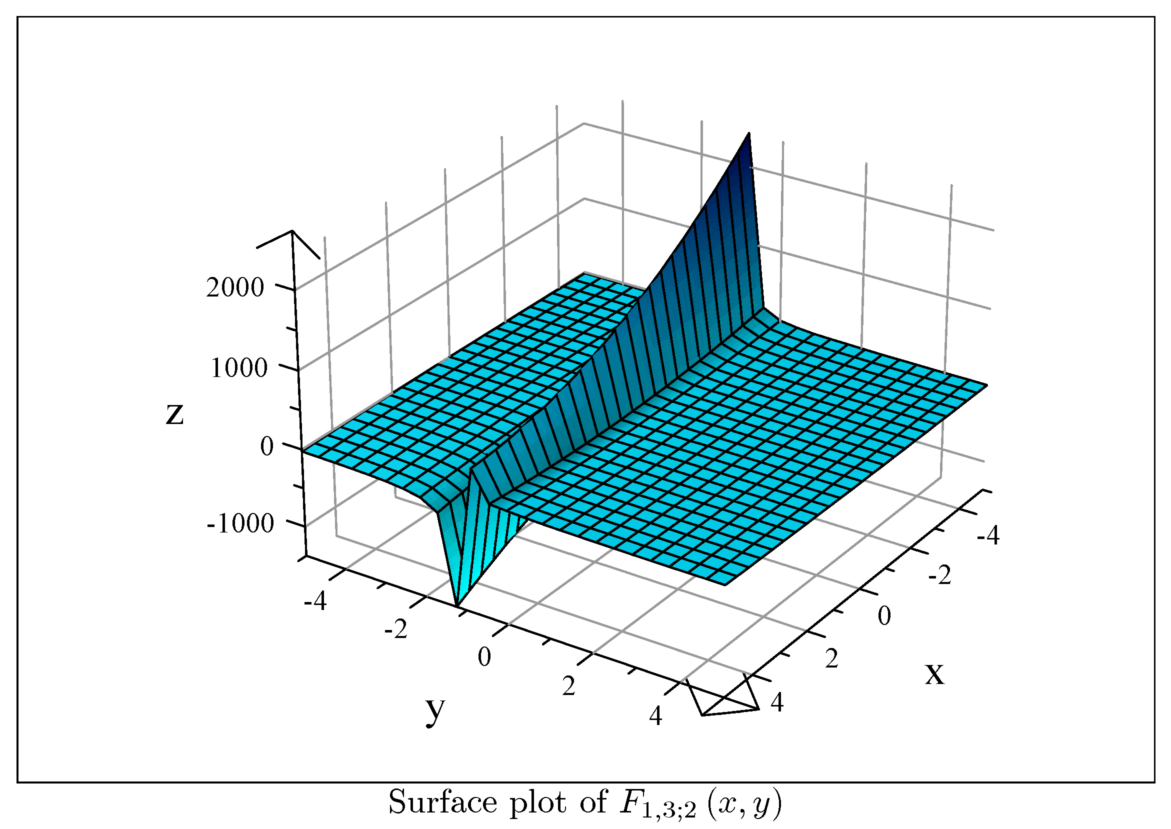
Moreover, upon letting $\lambda =2$ for the polynomials $F_{1,3;\lambda }\left(x,y\right)$, we then obtain

$$F_{1,3;2}\left(x,y\right)=\frac{6y^2}{{\left(y+1\right)}^3}+\frac{3y\left(-1+2x\right)}{{\left(y+1\right)}^2}+\frac{3\left(x^2-x\right)}{y+1}$$

which possess the following quirky surface plot in Figure 1.

Example 2.

By letting $m=2$ in (47), we obtain the following recurrence relation

$$F_{2,n+2;\lambda }\left(x,y\right)=\frac{y}{y+1}\sum _{j=0}^n\left(\genfrac{}{}{0pt}{}{n+2}{j}\right){\left(1\right)}_{n+2-j,\lambda }{F}_{2,j;\lambda }\left(x,y\right)+{\left(1\right)}_{2,\lambda }\frac{\left(n+2\right)\left(n+1\right)}{2}\frac{{\left(x\right)}_{n,\lambda }}{y+1}.$$

The last formula reveals the following polynomials

$$\begin{array}{c}{F}_{2,0;\lambda }\left(x,y\right)=F_{2,1;\lambda }\left(x,y\right)=0,\\ F_{2,2;\lambda }\left(x,y\right)=\frac{{\left(1\right)}_{2,\lambda }}{y+1},\\ F_{2,3;\lambda }\left(x,y\right)=\frac{3x{\left(1\right)}_{2,\lambda }}{y+1},\\ F_{2,4;\lambda }\left(x,y\right)=\frac{6y}{{\left(y+1\right)}^2}{\left({\left(1\right)}_{2,\lambda }\right)}^2+\frac{6{\left(1\right)}_{2,\lambda }{\left(x\right)}_{2,\lambda }}{y+1},\end{array}$$

which gives the following $Detr$-Fubini polynomials by taking $x=0$:

$$\begin{array}{c}{F}_{2,0;\lambda }\left(y\right)=F_{2,1;\lambda }\left(y\right)=0,\\ F_{2,2;\lambda }\left(y\right)=\frac{{\left(1\right)}_{2,\lambda }}{y+1},\\ F_{2,3;\lambda }\left(y\right)=\frac{3x{\left(1\right)}_{2,\lambda }}{y+1},\\ F_{2,4;\lambda }\left(y\right)=\frac{6y{\left(1\right)}_{2,\lambda }{\left(1\right)}_{2,\lambda }}{{\left(y+1\right)}^2}.\end{array}$$

By applying similar method used above, the others can be derived conveniently.

If we choose $\lambda =3$ for $F_{2,4;\lambda }\left(x,y\right)$, we then get

$$F_{2,4;\lambda }\left(x,y\right)=\frac{2y}{{\left(y+1\right)}^2}-\frac{12\left(x^2-3x\right)}{y+1}$$

which has the following interesting surface plot in Figure 2.

Here is a correlation between the bivariate $Detr$-Fubini polynomials and the degenerate Stirling numbers of the second kind.

Theorem 8.

For non-negative integer n and m, we have

$$F_{m,n;\lambda }\left(x,y\right)=\sum _{l=0}^n\sum _{k=0}^l\left(\genfrac{}{}{0pt}{}{n}{l}\right)F_{m,n-l;\lambda }\left(y\right)S_{2;\lambda }\left(l,k\right){\left(x\right)}_k.$$

(48)

Proof. 

By using the formula ([26])

$${\left(x\right)}_{n,\lambda }=\sum _{k=0}^n{S}_{2;\lambda }\left(n,k\right){\left(x\right)}_k$$

in conjunction with the Theorem 1, we derive

$$\begin{array}{ccc}\hfill F_{m,n;\lambda }\left(x,y\right)& =& \sum _{l=0}^n\left(\genfrac{}{}{0pt}{}{n}{l}\right)F_{m,n-l;\lambda }\left(y\right){\left(x\right)}_{l,\lambda }\hfill \\ & =& \sum _{l=0}^n\left(\genfrac{}{}{0pt}{}{n}{l}\right)F_{m,n-l;\lambda }\left(y\right)\sum _{k=0}^l{S}_{2;\lambda }\left(l,k\right){\left(x\right)}_k,\hfill \end{array}$$

which completes the proof of this theorem. □

Let n be a positive integer. The rising factorial for a number x is given by ${\left(x\right)}^{\left(n\right)}=x\left(x+1\right)\left(x+2\right)\cdots \left(x+n-1\right)$ ([9,27]). We note that the negative binomial expansion is given by the following series:

$${\left(x+a\right)}^{-n}=\sum _{k=0}^{\infty }{\left(-1\right)}^k\left(\genfrac{}{}{0pt}{}{n+k-1}{k}\right)x^k{a}^{-n-k}$$

(49)

for negative integer $-n$ and $\left|x\right|<a$, [9,27].

Here, we give the following theorem.

Theorem 9.

The following relationship

$$F_{m,n;\lambda }\left(x,y\right)=\sum _{k=0}^n\sum _{u=0}^n\left(\genfrac{}{}{0pt}{}{n}{u}\right)F_{m,n-u;}\left(y\right)S_{2;\lambda }\left(u,k:-k\right){\left(x\right)}^{\left(k\right)}$$

(50)

holds true for non-negative integers n and m.

Proof. 

By means of the Definition 3 and in terms of Equations (26) and (49), we attain

$$\begin{array}{ccc}\hfill \sum _{n=0}^{\infty }{F}_{m,n;\lambda }\left(x,y\right)\frac{t^n}{n!}& =& \frac{{\left(1\right)}_{m,\lambda }\frac{t^m}{m!}}{1-y\left(e_{\lambda }\left(t\right)-1-e_{m-1,\lambda }\left(t\right)\right)}{\left(e_{\lambda }^{-1}\left(t\right)-1+1\right)}^x\hfill \\ & =& \frac{{\left(1\right)}_{m,\lambda }\frac{t^m}{m!}}{1-y\left(e_{\lambda }\left(t\right)-1-e_{m-1,\lambda }\left(t\right)\right)}\sum _{k=0}^{\infty }\left(\genfrac{}{}{0pt}{}{x+k-1}{k}\right){\left(1-e_{\lambda }^{-1}\left(t\right)\right)}^k\hfill \\ & =& \frac{{\left(1\right)}_{m,\lambda }\frac{t^m}{m!}}{1-y\left(e_{\lambda }\left(t\right)-1-e_{m-1,\lambda }\left(t\right)\right)}\sum _{k=0}^{\infty }\left(\genfrac{}{}{0pt}{}{x+k-1}{k}\right)\frac{{\left(e_{\lambda }\left(t\right)-1\right)}^k}{k!}{e}_{\lambda }^{-k}\left(t\right)k!\hfill \\ & =& \sum _{k=0}^{\infty }{\left(x\right)}^{\left(k\right)}\sum _{n=0}^{\infty }{F}_{m,n;\lambda }\left(y\right)\frac{t^n}{n!}\sum _{n=0}^{\infty }{S}_{2;\lambda }\left(n,k:-k\right)\frac{t^n}{n!}\hfill \\ & =& \sum _{k=0}^{\infty }{\left(x\right)}^{\left(k\right)}\sum _{n=0}^{\infty }\left(\sum _{u=0}^n\left(\genfrac{}{}{0pt}{}{n}{u}\right)F_{m,n-u;\lambda }\left(y\right)S_{2;\lambda }\left(u,k:-k\right)\right)\frac{t^n}{n!},\hfill \end{array}$$

which gives the asserted result (50). □

We give the following theorem.

Theorem 10.

The following recurrence relationship

$$F_{m+1,n;\lambda }\left(x,y\right)=n\frac{1-m\lambda }{m+1}{F}_{m,n-1;\lambda }\left(x,y\right)-y\sum _{k=0}^n\left(\genfrac{}{}{0pt}{}{n}{k}\right)F_{m,n-k;\lambda }\left(y\right)F_{m+1,k;\lambda }\left(x,y\right)$$

(51)

holds true for $n,m\in {\mathbb{N}}_0$.

Proof. 

With the help of the Definition 3, we see that

$$\begin{array}{c}{\left(1\right)}_{m+1,\lambda }\frac{t^{m+1}}{\left(m+1\right)!}{e}_{\lambda }^x\left(t\right)=\left(1-y\left(e_{\lambda }\left(t\right)-1-e_{m,\lambda }\left(t\right)\right)\right)\sum _{n=0}^{\infty }{F}_{m+1,n;\lambda }\left(x,y\right)\frac{t^n}{n!}\\ =\left(1-y\left(e_{\lambda }\left(t\right)-1-e_{m-1,\lambda }\left(t\right)\right)\right)\sum _{n=0}^{\infty }{F}_{m+1,n;\lambda }\left(x,y\right)\frac{t^n}{n!}\\ +y{\left(1\right)}_{m,\lambda }\frac{t^m}{m!}\sum _{n=0}^{\infty }{F}_{m+1,n;\lambda }\left(x,y\right)\frac{t^n}{n!}.\end{array}$$

Thus, we get

$$\begin{array}{c}\frac{{\left(1\right)}_{m+1,\lambda }\frac{t^{m+1}}{\left(m+1\right)!}}{\left(1-y\left(e_{\lambda }\left(t\right)-1-e_{m-1,\lambda }\left(t\right)\right)\right)}{e}_{\lambda }^x\left(t\right)=\sum _{n=0}^{\infty }{F}_{m+1,n;\lambda }\left(x,y\right)\frac{t^n}{n!}\\ +y\frac{{\left(1\right)}_{m,\lambda }\frac{t^m}{m!}}{\left(1-y\left(e_{\lambda }\left(t\right)-1-e_{m-1,\lambda }\left(t\right)\right)\right)}\sum _{n=0}^{\infty }{F}_{m+1,n;\lambda }\left(x,y\right)\frac{t^n}{n!}\end{array}$$

and then

$$\begin{array}{c}\frac{1-m\lambda }{m+1}\sum _{n=0}^{\infty }{F}_{m,n;\lambda }\left(x,y\right)\frac{t^{n+1}}{n!}=\sum _{n=0}^{\infty }{F}_{m+1,n;\lambda }\left(x,y\right)\frac{t^n}{n!}\\ +y\sum _{n=0}^{\infty }{F}_{m,n;\lambda }\left(y\right)\frac{t^n}{n!}\sum _{n=0}^{\infty }{F}_{m+1,n;\lambda }\left(x,y\right)\frac{t^n}{n!},\end{array}$$

which implies the claimed Formula (51). □

A linear combination of the bivariate $Detr$-Fubini polynomials for different x and y values is given by the following theorem.

Theorem 11.

Let $n,m\in {\mathbb{N}}_0$ and $y_1\ne y_2$. The following relationship holds true:

$$\begin{array}{cc}& \sum _{k=0}^{n+m}\frac{n!m!}{\left(n+m-k\right)!k!}{F}_{m,n+m-k}\left(x_1,y_1\right)F_{m,k}\left(x_2,y_2\right)\hfill \\ =& {\left(1\right)}_{m,\lambda }\frac{y_2{F}_{m,n;\lambda }\left(x_1+x_2,y_2\right)-y_1{F}_{m,n;\lambda }\left(x_1+x_2,y_1\right)}{y_2-y_1}.\hfill \end{array}$$

(52)

Proof. 

By Definition 3, we first consider the following product

$$\begin{array}{c}\frac{{\left(1\right)}_{m,\lambda }\frac{t^m}{m!}{e}_{\lambda }^{x_1}\left(t\right)}{1-y_1\left(e_{\lambda }\left(t\right)-1-e_{m-1,\lambda }\left(t\right)\right)}\frac{{\left(1\right)}_{m,\lambda }\frac{t^m}{m!}{e}_{\lambda }^{x_2}\left(t\right)}{1-y_2\left(e_{\lambda }\left(t\right)-1-e_{m-1,\lambda }\left(t\right)\right)}\\ =\frac{y_2}{y_2-y_1}\frac{{\left({\left(1\right)}_{m,\lambda }\right)}^2\frac{t^{2m}}{{\left(m!\right)}^2}{e}_{\lambda }^{x_1+x_2}\left(t\right)}{1-y_2\left(e_{\lambda }\left(t\right)-1-e_{m-1,\lambda }\left(t\right)\right)}-\frac{y_1}{y_2-y_1}\frac{{\left({\left(1\right)}_{m,\lambda }\right)}^2\frac{t^{2m}}{{\left(m!\right)}^2}{e}_{\lambda }^{x_1+x_2}\left(t\right)}{1-y_1\left(e_{\lambda }\left(t\right)-1-e_{m-1,\lambda }\left(t\right)\right)},\end{array}$$

which yields

$$\begin{array}{cc}& \sum _{n=0}^{\infty }\sum _{l=0}^n\left(\genfrac{}{}{0pt}{}{n}{l}\right)F_{m,n-l;\lambda }\left(x_1,y_1\right)F_{m,l;\lambda }\left(x_2,y_2\right)\frac{t^n}{n!}\hfill \\ =& \frac{{\left(1\right)}_{m,\lambda }{y}_2}{y_2-y_1}\sum _{n=0}^{\infty }{F}_{m,n;\lambda }\left(x_1+x_2,y_2\right)\frac{t^{n+m}}{n!m!}-\frac{{\left(1\right)}_{m,\lambda }{y}_1}{y_2-y_1}\sum _{n=0}^{\infty }{F}_{m,n;\lambda }\left(x_1+x_2,y_1\right)\frac{t^{n+m}}{n!m!}.\hfill \end{array}$$

Thus, we get

$$\begin{array}{cc}& \sum _{n=0}^{\infty }\left(\sum _{l=0}^n\left(\genfrac{}{}{0pt}{}{n}{l}\right)F_{m,n-l;\lambda }\left(x_1,y_1\right)F_{m,l;\lambda }\left(x_2,y_2\right)\right)\frac{t^n}{n!}\hfill \\ =& \sum _{n=0}^{\infty }\left(\frac{{\left(1\right)}_{m,\lambda }{y}_2}{y_2-y_1}{F}_{m,n;\lambda }\left(x_1+x_2,y_2\right)-\frac{{\left(1\right)}_{m,\lambda }{y}_1}{y_2-y_1}{F}_{m,n;\lambda }\left(x_1+x_2,y_1\right)\right)\frac{t^{n+m}}{n!m!},\hfill \end{array}$$

which implies the assertion in (52). □

5. The Truncated Degenerate Bernoulli and Euler Polynomials

In this section, we introduce the truncated degenerate Bernoulli and Euler polynomials and investigated multifarious correlations and formulas including summation formulas, derivation rules and correlations with the degenerate truncated Stirling numbers of the second kind.

The classical Bernoulli $B_n\left(x\right)$ and Euler $E_n\left(x\right)$ polynomials ([6,13,27,35]) and the Apostol-type Bernoulli $B_n\left(x:\alpha \right)$ and the Apostol-type Euler $E_n\left(x:\alpha \right)$ polynomials ([2,7,31,33,34]) are given as follows:

$$\begin{array}{cc}{\displaystyle \sum _{n=0}^{\infty }}{B}_n\left(x\right)\frac{t^n}{n!}=\frac{t}{e^t-1}{e}^{xt}& {\displaystyle \sum _{n=0}^{\infty }}{B}_n\left(x:\alpha \right)\frac{t^n}{n!}=\frac{t}{\alpha e^t-1}{e}^{xt}\\ \left(\left|t\right|<2\pi \right)& \left(\left|t\right|<2\pi \mathrm{when}\alpha =1;\left|t\right|<\left|log\alpha \right|\mathrm{when}\alpha \ne 1\right)\end{array}$$

and

$$\begin{array}{cc}{\displaystyle \sum _{n=0}^{\infty }}{E}_n\left(x\right)\frac{t^n}{n!}=\frac{2}{e^t+1}{e}^{xt}& {\displaystyle \sum _{n=0}^{\infty }}{E}_n\left(x:\alpha \right)\frac{t^n}{n!}=\frac{2}{\alpha e^t+1}{e}^{xt}\\ \left(\left|t\right|<\pi \right)& \left(\left|t\right|<\pi \mathrm{when}\alpha =1;\left|t\right|<\left|log\left(-\alpha \right)\right|\mathrm{when}\alpha \ne 1\right).\end{array}$$

The usual degenerate Bernoulli $B_{n,\lambda }\left(x\right)$ and Euler $E_{n,\lambda }\left(x\right)$ polynomials ([5,11,14,32]) and Apostol-type degenerate Bernoulli $B_{n,\lambda }\left(x:\alpha \right)$ and Euler $E_{n,\lambda }\left(x:\alpha \right)$ polynomials are given as follows ([32]):

$$\begin{array}{ccc}\hfill \sum _{n=0}^{\infty }{B}_{n,\lambda }\left(x\right)\frac{t^n}{n!}& =& \frac{t}{e_{\lambda }\left(t\right)-1}{e}_{\lambda }^x\left(t\right)\mathrm{and}\sum _{n=0}^{\infty }{B}_{n,\lambda }\left(x:\alpha \right)\frac{t^n}{n!}=\frac{t}{\alpha e_{\lambda }\left(t\right)-1}{e}_{\lambda }^x\left(t\right)\hfill \\ \hfill \sum _{n=0}^{\infty }{E}_{n,\lambda }\left(x\right)\frac{t^n}{n!}& =& \frac{2}{e_{\lambda }\left(t\right)+1}{e}_{\lambda }^x\left(t\right)\mathrm{and}\sum _{n=0}^{\infty }{E}_{n,\lambda }\left(x:\alpha \right)\frac{t^n}{n!}=\frac{2}{\alpha e_{\lambda }\left(t\right)+1}{e}_{\lambda }^x\left(t\right).\hfill \end{array}$$

The truncated Bernoulli polynomials $B_{m,n}\left(x\right)$ and the truncated Euler polynomials $E_{m,n}\left(x\right)$ are defined by the following exponential generating functions ([9,13,27]):

$$\sum _{n=0}^{\infty }{B}_{m,n}\left(x\right)\frac{t^n}{n!}=\frac{\frac{t^{m+1}}{\left(m+1\right)!}}{e^t-1-e_{m-1}\left(t\right)}{e}^{xt}$$

(53)

and

$$\sum _{n=0}^{\infty }{E}_{m,n}\left(x\right)\frac{t^n}{n!}=\frac{2\frac{t^m}{m!}}{e^t+1-e_{m-1}\left(t\right)}{e}^{xt}.$$

(54)

Several degenerate and truncated forms of the Bernoulli and Euler polynomials have been recently studied and investigated by many mathematicians, [5,9,11,13,14,27,32].

We now introduce the degenerate forms of the truncated Bernoulli and the truncated Euler polynomials by means of the degenerate exponential function in (11) as follows.

Definition 4.

Let x be an independent variable. The degenerate truncated Bernoulli and the degenerate truncated Euler polynomials are defined by the following exponential generating functions:

$$\sum _{n=0}^{\infty }{B}_{m,n,\lambda }\left(x\right)\frac{t^n}{n!}=\frac{{\left(1\right)}_{m+1,\lambda }\frac{t^{m+1}}{\left(m+1\right)!}}{e_{\lambda }\left(t\right)-1-e_{m-1,\lambda }\left(t\right)}{e}_{\lambda }^x\left(t\right)$$

(55)

and

$$\sum _{n=0}^{\infty }{E}_{m,n,\lambda }\left(x\right)\frac{t^n}{n!}=\frac{2\frac{t^m}{m!}{\left(1\right)}_{m,\lambda }}{e_{\lambda }\left(t\right)+1-e_{m-1,\lambda }\left(t\right)}{e}_{\lambda }^x\left(t\right).$$

(56)

We choose to call the $Detr$-Bernoulli and $Detr$-Euler polynomials besides the degenerate truncated Bernoulli and the degenerate truncated Euler polynomials, respectively.

When $x=0$ in Definition 4, the $Detr$-Bernoulli polynomials $B_{m,n,\lambda }\left(x\right)$ and $Detr$-Euler polynomials $E_{m,n,\lambda }\left(x\right)$ reduce to the corresponding numbers called the $Detr$-Bernoulli numbers denoted by $B_{m,n,\lambda }$ and the $Detr$-Euler numbers denoted by $E_{m,n,\lambda }$:

$$\sum _{n=0}^{\infty }{B}_{m,n,\lambda }\frac{t^n}{n!}=\frac{{\left(1\right)}_{m+1,\lambda }\frac{t^{m+1}}{\left(m+1\right)!}}{e_{\lambda }\left(t\right)-1-e_{m-1,\lambda }\left(t\right)}$$

(57)

and

$$\sum _{n=0}^{\infty }{E}_{m,n,\lambda }\frac{t^n}{n!}=\frac{2\frac{t^m}{m!}{\left(1\right)}_{m,\lambda }}{e_{\lambda }\left(t\right)+1-e_{m-1,\lambda }\left(t\right)}.$$

(58)

We now perform to derive some properties of the aforementioned polynomials and we first give the following correlations.

Theorem 12.

Each of the following summation formulas

$$B_{m,n,\lambda }\left(x\right)=\sum _{k=0}^n\left(\genfrac{}{}{0pt}{}{n}{k}\right){\left(x\right)}_{k,\lambda }{B}_{m,n-k,\lambda }$$

(59)

and

$$E_{m,n,\lambda }\left(x\right)=\sum _{k=0}^n\left(\genfrac{}{}{0pt}{}{n}{k}\right){\left(x\right)}_{k,\lambda }{E}_{m,n-k,\lambda }$$

(60)

hold true.

Proof. 

In view of the Definition 4 and using Formulas (57) and (58), we get

$$\begin{array}{ccc}\hfill \sum _{n=0}^{\infty }{B}_{m,n,\lambda }\left(x\right)\frac{t^n}{n!}& =& \frac{{\left(1\right)}_{m+1,\lambda }\frac{t^{m+1}}{\left(m+1\right)!}}{e_{\lambda }\left(t\right)-1-e_{m-1,\lambda }\left(t\right)}{e}_{\lambda }^x\left(t\right)\hfill \\ & =& \sum _{n=0}^{\infty }{B}_{m,n,\lambda }\frac{t^n}{n!}\sum _{n=0}^{\infty }{\left(x\right)}_{n,\lambda }\frac{t^n}{n!}\hfill \\ & =& \sum _{n=0}^{\infty }\sum _{k=0}^n\left(\genfrac{}{}{0pt}{}{n}{k}\right){\left(x\right)}_{k,\lambda }{B}_{m,n-k,\lambda }\frac{t^n}{n!}\hfill \end{array}$$

and

$$\begin{array}{ccc}\hfill \sum _{n=0}^{\infty }{E}_{m,n,\lambda }\left(x\right)\frac{t^n}{n!}& =& \frac{2\frac{t^m}{m!}{\left(1\right)}_{m,\lambda }}{e_{\lambda }\left(t\right)+1-e_{m-1,\lambda }\left(t\right)}{e}_{\lambda }^x\left(t\right)\hfill \\ & =& \sum _{n=0}^{\infty }{E}_{m,n,\lambda }\frac{t^n}{n!}\sum _{n=0}^{\infty }{\left(x\right)}_{n,\lambda }\frac{t^n}{n!}\hfill \\ & =& \sum _{n=0}^{\infty }\sum _{k=0}^n\left(\genfrac{}{}{0pt}{}{n}{k}\right){\left(x\right)}_{k,\lambda }{E}_{m,n-k,\lambda }\frac{t^n}{n!},\hfill \end{array}$$

which completes the proof of the Theorem 12. □

Two addition formulas for the $Detr$-Bernoulli polynomials and $Detr$-Euler polynomials are presented in the following theorem.

Theorem 13.

The following relationships

$$B_{m,n,\lambda }\left(x_1+x_2\right)=\sum _{l=0}^n\left(\genfrac{}{}{0pt}{}{n}{l}\right){\left(x_2\right)}_{n-l,\lambda }{B}_{m,l,\lambda }\left(x_1\right)$$

(61)

and

$$E_{m,n,\lambda }\left(x_1+x_2\right)=\sum _{l=0}^n\left(\genfrac{}{}{0pt}{}{n}{l}\right){\left(x_2\right)}_{n-l,\lambda }{E}_{m,l,\lambda }\left(x_1\right)$$

(62)

are valid.

Proof. 

In terms of the Definition 4 and using Formulas (57) and (58), we get

$$\begin{array}{ccc}\hfill \sum _{n=0}^{\infty }{B}_{m,n,\lambda }\left(x_1+x_2\right)\frac{t^n}{n!}& =& \frac{{\left(1\right)}_{m+1,\lambda }\frac{t^{m+1}}{\left(m+1\right)!}}{e_{\lambda }\left(t\right)-1-e_{m-1,\lambda }\left(t\right)}{e}_{\lambda }^{x_1+x_2}\left(t\right)\hfill \\ & =& \sum _{n=0}^{\infty }{B}_{m,n,\lambda }\left(x_1\right)\frac{t^n}{n!}\sum _{n=0}^{\infty }{\left(x_2\right)}_{n,\lambda }\frac{t^n}{n!}\hfill \\ & =& \sum _{n=0}^{\infty }\sum _{l=0}^n\left(\genfrac{}{}{0pt}{}{n}{l}\right){\left(x_2\right)}_{n-l,\lambda }{B}_{m,l,\lambda }\left(x_1\right)\frac{t^n}{n!}\hfill \end{array}$$

and

$$\begin{array}{ccc}\hfill \sum _{n=0}^{\infty }{E}_{m,n,\lambda }\left(x_1+x_2\right)\frac{t^n}{n!}& =& \frac{2\frac{t^m}{m!}{\left(1\right)}_{m,\lambda }}{e_{\lambda }\left(t\right)+1-e_{m-1,\lambda }\left(t\right)}{e}_{\lambda }^{x_1+x_2}\left(t\right)\hfill \\ & =& \sum _{n=0}^{\infty }{E}_{m,n,\lambda }\left(x_1\right)\frac{t^n}{n!}\sum _{n=0}^{\infty }{\left(x_2\right)}_{n,\lambda }\frac{t^n}{n!}\hfill \\ & =& \sum _{n=0}^{\infty }\sum _{l=0}^n\left(\genfrac{}{}{0pt}{}{n}{l}\right){\left(x_2\right)}_{n-l,\lambda }{E}_{m,l,\lambda }\left(x_1\right)\frac{t^n}{n!},\hfill \end{array}$$

which implies Formulas (61) and (62). □

The immediate special cases of the Theorem 13 is debated below.

Corollary 1.

The following explicit relations

$$B_{m,n,\lambda }\left(x+1\right)=\sum _{l=0}^n\left(\genfrac{}{}{0pt}{}{n}{l}\right){\left(1\right)}_{n-l,\lambda }{B}_{m,l,\lambda }\left(x\right)$$

(63)

and

$$E_{m,n,\lambda }\left(x+1\right)=\sum _{l=0}^n\left(\genfrac{}{}{0pt}{}{n}{l}\right){\left(1\right)}_{n-l,\lambda }{E}_{m,l,\lambda }\left(x\right)$$

(64)

hold true.

We now provide difference operator properties for the polynomials $B_{m,n,\lambda }\left(x\right)$ and $E_{m,n,\lambda }\left(x\right)$ as follows.

Theorem 14.

The difference operator formulas for the $Detr$-Bernoulli and $Detr$-Euler polynomials

$${\mathsf{\Delta }}_{\lambda }{B}_{m,n,\lambda }\left(x\right)=n{B}_{m,n-1,\lambda }\left(x\right)\mathrm{and}{\mathsf{\Delta }}_{\lambda }{E}_{m,n,\lambda }\left(x\right)=n{E}_{m,n-1,\lambda }\left(x\right)$$

(65)

hold true for $m,n\in {\mathbb{N}}_0$.

Proof. 

By applying difference operator ${\mathsf{\Delta }}_{\lambda }$ (12) to both sides of Formulas (55) and (56), respectively, we attain

$$\begin{array}{ccc}\hfill \sum _{n=0}^{\infty }{\mathsf{\Delta }}_{\lambda }{B}_{m,n,\lambda }\left(x\right)\frac{t^n}{n!}& =& \frac{{\left(1\right)}_{m+1,\lambda }\frac{t^{m+1}}{\left(m+1\right)!}}{e_{\lambda }\left(t\right)-1-e_{m-1,\lambda }\left(t\right)}{\mathsf{\Delta }}_{\lambda }{e}_{\lambda }^x\left(t\right)\hfill \\ & =& \frac{{\left(1\right)}_{m+1,\lambda }\frac{t^{m+1}}{\left(m+1\right)!}{e}_{\lambda }^x\left(t\right)}{e_{\lambda }\left(t\right)-1-e_{m-1,\lambda }\left(t\right)}t\hfill \\ & =& \sum _{n=0}^{\infty }{B}_{m,n,\lambda }\left(x\right)\frac{t^{n+1}}{n!},\hfill \end{array}$$

and

$$\begin{array}{ccc}\hfill \sum _{n=0}^{\infty }{\mathsf{\Delta }}_{\lambda }{E}_{m,n,\lambda }\left(x\right)\frac{t^n}{n!}& =& \frac{{\left(1\right)}_{m,\lambda }\frac{t^m}{m!}}{e_{\lambda }\left(t\right)+1-e_{m-1,\lambda }\left(t\right)}{\mathsf{\Delta }}_{\lambda }{e}_{\lambda }^x\left(t\right)\hfill \\ & =& \frac{{\left(1\right)}_{m,\lambda }\frac{t^m}{m!}{e}_{\lambda }^x\left(t\right)}{e_{\lambda }\left(t\right)+1-e_{m-1,\lambda }\left(t\right)}t\hfill \\ & =& \sum _{n=0}^{\infty }{E}_{m,n,\lambda }\left(x\right)\frac{t^{n+1}}{n!},\hfill \end{array}$$

which gives the claimed difference properties in (65). □

The $Detr$-Bernoulli polynomials and the $Detr$-Euler polynomials satisfy the following derivative properties.

Theorem 15.

We have

$$\frac{d}{dx}{B}_{m,n;\lambda }\left(x\right)=n!\sum _{u=1}^{\infty }{B}_{m,n-u;\lambda }\left(x\right)\frac{{\left(-1\right)}^{u+1}}{\left(n-u\right)!u}{\lambda }^{u-1}$$

(66)

and

$$\frac{d}{dx}{E}_{m,n;\lambda }\left(x\right)=n!\sum _{u=1}^{\infty }{E}_{m,n-u;\lambda }\left(x\right)\frac{{\left(-1\right)}^{u+1}}{\left(n-u\right)!u}{\lambda }^{u-1}.$$

(67)

Proof. 

By using the similar proof method in Theorem 6, the proof of (66) and (67) can be readily done. We, consequently, choose to omit details involved. □

A recurrence relation for the $Detr$-Bernoulli polynomials is given by the following theorem.

Theorem 16.

The following recurrence relationship

$$B_{m+1,n,\lambda }\left(x\right)=n\frac{1-\left(m+1\right)\lambda }{m+2}{B}_{m,n-1;\lambda }\left(x\right)+\sum _{k=0}^n\left(\genfrac{}{}{0pt}{}{n}{k}\right)B_{m,n-k;\lambda }{B}_{m+1,k;\lambda }\left(x\right)$$

(68)

holds true for $n,m\in {\mathbb{N}}_0$.

Proof. 

By means of the Definition 4, we see that

$$\begin{array}{c}{\left(1\right)}_{m+2,\lambda }\frac{t^{m+2}}{\left(m+2\right)!}{e}_{\lambda }^x\left(t\right)=\left(e_{\lambda }\left(t\right)-1-e_{m,\lambda }\left(t\right)\right)\sum _{n=0}^{\infty }{B}_{m+1,n,\lambda }\left(x\right)\frac{t^n}{n!}\\ =\left(e_{\lambda }\left(t\right)-1-e_{m-1,\lambda }\left(t\right)\right)\sum _{n=0}^{\infty }{B}_{m+1,n,\lambda }\left(x\right)\frac{t^n}{n!}\\ {\left(1\right)}_{m,\lambda }\frac{t^m}{m!}\sum _{n=0}^{\infty }{B}_{m+1,n,\lambda }\left(x\right)\frac{t^n}{n!}\end{array}$$

Thus, we get

$$\begin{array}{c}\frac{{\left(1\right)}_{m+2,\lambda }\frac{t^{m+2}}{\left(m+2\right)!}}{e_{\lambda }\left(t\right)-1-e_{m-1,\lambda }\left(t\right)}{e}_{\lambda }^x\left(t\right)=\sum _{n=0}^{\infty }{B}_{m+1,n,\lambda }\left(x\right)\frac{t^n}{n!}\\ -\frac{{\left(1\right)}_{m,\lambda }\frac{t^m}{m!}}{e_{\lambda }\left(t\right)-1-e_{m-1,\lambda }\left(t\right)}\sum _{n=0}^{\infty }{B}_{m+1,n,\lambda }\left(x\right)\frac{t^n}{n!}\end{array}$$

and then

$$\begin{array}{c}\frac{1-\left(m+1\right)\lambda }{m+2}\sum _{n=0}^{\infty }{B}_{m,n,\lambda }\left(x\right)\frac{t^{n+1}}{n!}=\sum _{n=0}^{\infty }{B}_{m+1,n,\lambda }\left(x\right)\frac{t^n}{n!}\\ -\sum _{n=0}^{\infty }{B}_{m,n,\lambda }\frac{t^n}{n!}\sum _{n=0}^{\infty }{B}_{m+1,n,\lambda }\left(x\right)\frac{t^n}{n!}.\end{array}$$

which implies the claimed Formula (51). □

A summation identity for the $Detr$-Euler polynomials is presented in the following theorem.

Theorem 17.

The following recurrence formula

$$E_{m+1,n,\lambda }\left(x\right)=n\frac{1-m\lambda }{m+1}{E}_{m,n-1;\lambda }\left(x\right)+\sum _{k=0}^n\left(\genfrac{}{}{0pt}{}{n}{k}\right)E_{m,n-k;\lambda }{E}_{m+1,k;\lambda }\left(x\right)$$

(69)

is valid for $n,m\in {\mathbb{N}}_0$.

Proof. 

From Definition 3, we can write

$$\begin{array}{c}2\frac{t^{m+1}}{\left(m+1\right)!}{\left(1\right)}_{m+1,\lambda }{e}_{\lambda }^x\left(t\right)=\left(e_{\lambda }\left(t\right)+1-e_{m,\lambda }\left(t\right)\right)\sum _{n=0}^{\infty }{E}_{m+1,n,\lambda }\left(x\right)\frac{t^n}{n!}\\ =\left(e_{\lambda }\left(t\right)+1-e_{m-1,\lambda }\left(t\right)\right)\sum _{n=0}^{\infty }{E}_{m+1,n,\lambda }\left(x\right)\frac{t^n}{n!}\\ {\left(1\right)}_{m,\lambda }\frac{t^m}{m!}\sum _{n=0}^{\infty }{E}_{m+1,n,\lambda }\left(x\right)\frac{t^n}{n!}\end{array}$$

Hence, we observe that

$$\begin{array}{c}\frac{\frac{t^{m+1}}{\left(m+1\right)!}{\left(1\right)}_{m+1,\lambda }}{e_{\lambda }\left(t\right)+1-e_{m-1,\lambda }\left(t\right)}{e}_{\lambda }^x\left(t\right)=\sum _{n=0}^{\infty }{E}_{m+1,n,\lambda }\left(x\right)\frac{t^n}{n!}\\ -\frac{{\left(1\right)}_{m,\lambda }\frac{t^m}{m!}}{e_{\lambda }\left(t\right)-1-e_{m-1,\lambda }\left(t\right)}\sum _{n=0}^{\infty }{E}_{m+1,n,\lambda }\left(x\right)\frac{t^n}{n!}\end{array}$$

and

$$\begin{array}{c}\frac{1-m\lambda }{m+1}\sum _{n=0}^{\infty }{E}_{m,n,\lambda }\left(x\right)\frac{t^{n+1}}{n!}=\sum _{n=0}^{\infty }{E}_{m+1,n,\lambda }\left(x\right)\frac{t^n}{n!}\\ -\sum _{n=0}^{\infty }{E}_{m,n,\lambda }\frac{t^n}{n!}\sum _{n=0}^{\infty }{E}_{m+1,n,\lambda }\left(x\right)\frac{t^n}{n!}.\end{array}$$

which means the asserted result (69). □

We give the following theorem.

Theorem 18.

The following formula including the $Detr$-Bernoulli polynomials

$$\frac{{\left(1\right)}_{m+1,\lambda }}{\left(m+1\right)!}{\left(x\right)}_{n,\lambda }=\sum _{k=0}^{n+1}\frac{n!{\left(1\right)}_{k+m,\lambda }{B}_{m,n+1-k,\lambda }\left(x\right)}{\left(k+m\right)!\left(n+1-k\right)!}-\frac{n!B_{m,n+m+1,\lambda }\left(x\right)}{\left(n+m+1\right)!}$$

(70)

is valid for $n,m\in {\mathbb{N}}_0$.

Proof. 

From Definition 3, we obtain

$$\begin{array}{ccc}\hfill {\left(1\right)}_{m+1,\lambda }\frac{t^{m+1}}{\left(m+1\right)!}{e}_{\lambda }^x\left(t\right)& =& \left(e_{\lambda }\left(t\right)-1-e_{m-1,\lambda }\left(t\right)\right)\sum _{n=0}^{\infty }{B}_{m,n,\lambda }\left(x\right)\frac{t^n}{n!}\hfill \\ & =& \sum _{n=m}^{\infty }{\left(1\right)}_{n,\lambda }\frac{t^n}{n!}\sum _{n=0}^{\infty }{B}_{m,n,\lambda }\left(x\right)\frac{t^n}{n!}-\sum _{n=0}^{\infty }{B}_{m,n,\lambda }\left(x\right)\frac{t^n}{n!},\hfill \end{array}$$

which yields to the following equality:

$$\begin{array}{ccc}\hfill \sum _{n=0}^{\infty }{\left(x\right)}_{n,\lambda }\frac{{\left(1\right)}_{m+1,\lambda }}{\left(m+1\right)!}\frac{t^{n+m+1}}{n!}& =& \sum _{n=0}^{\infty }{\left(1\right)}_{n+m,\lambda }\frac{t^{n+m}}{\left(n+m\right)!}\sum _{n=0}^{\infty }{B}_{m,n,\lambda }\left(x\right)\frac{t^n}{n!}\hfill \\ & & -\sum _{n=0}^{\infty }{B}_{m,n,\lambda }\left(x\right)\frac{t^n}{n!}\hfill \\ & =& \sum _{n=0}^{\infty }\left(\sum _{k=0}^n\frac{{\left(1\right)}_{k+m,\lambda }}{\left(k+m\right)!\left(n-k\right)!}{B}_{m,n-k,\lambda }\left(x\right)\right)t^{n+m}\hfill \\ & & -\sum _{n=0}^{\infty }{B}_{m,n,\lambda }\left(x\right)\frac{t^n}{n!}.\hfill \end{array}$$

Thus, we complete the proof just comparing the coefficients of the both sides of the last equality. □

We note that Formula (70) is an extension of the well-known formula for the familiar Bernoulli polynomials given by ([6]):

$$x^n=\frac{1}{n+1}\sum _{l=0}^n\left(\genfrac{}{}{0pt}{}{n+1}{l}\right)B_k\left(x\right).$$

We provide an identity for $Detr$-Euler polynomials as follows.

Theorem 19.

The following identity

$$2\frac{{\left(1\right)}_{m,\lambda }}{m!}{\left(x\right)}_{n,\lambda }=\frac{n!}{2}\sum _{k=0}^n\frac{{\left(1\right)}_{k+m,\lambda }}{\left(k+m\right)!\left(n-k\right)!}{E}_{m,n-k,\lambda }\left(x\right)+\frac{n!}{2}\frac{E_{m,n+m,\lambda }\left(x\right)}{\left(n+m\right)!}$$

(71)

is true for $n,m\in {\mathbb{N}}_0$.

Proof. 

From Definition 3, we obtain ${\sum }_{n=0}^{\infty }{E}_{m,n,\lambda }\left(x\right)\frac{t^n}{n!}=\frac{2\frac{t^m}{m!}{\left(1\right)}_{m,\lambda }}{e_{\lambda }\left(t\right)+1-e_{m-1,\lambda }\left(t\right)}{e}_{\lambda }^x\left(t\right)$

$$\begin{array}{ccc}\hfill 2\frac{t^m}{m!}{\left(1\right)}_{m,\lambda }{e}_{\lambda }^x\left(t\right)& =& \left(e_{\lambda }\left(t\right)+1-e_{m-1,\lambda }\left(t\right)\right)\sum _{n=0}^{\infty }{E}_{m,n,\lambda }\left(x\right)\frac{t^n}{n!}\hfill \\ & =& \sum _{n=m}^{\infty }{\left(1\right)}_{n,\lambda }\frac{t^n}{n!}\sum _{n=0}^{\infty }{E}_{m,n,\lambda }\left(x\right)\frac{t^n}{n!}+\sum _{n=0}^{\infty }{E}_{m,n,\lambda }\left(x\right)\frac{t^n}{n!},\hfill \end{array}$$

which yields to the following equality:

$$\begin{array}{ccc}\hfill \sum _{n=0}^{\infty }2{\left(x\right)}_{n,\lambda }\frac{{\left(1\right)}_{m,\lambda }}{m!}\frac{t^{n+m}}{n!}& =& \sum _{n=0}^{\infty }{\left(1\right)}_{n+m,\lambda }\frac{t^{n+m}}{\left(n+m\right)!}\sum _{n=0}^{\infty }{E}_{m,n,\lambda }\left(x\right)\frac{t^n}{n!}\hfill \\ & & +\sum _{n=0}^{\infty }{E}_{m,n,\lambda }\left(x\right)\frac{t^n}{n!}\hfill \\ & =& \sum _{n=0}^{\infty }\left(\sum _{k=0}^n\frac{{\left(1\right)}_{k+m,\lambda }}{\left(k+m\right)!\left(n-k\right)!}{E}_{m,n-k,\lambda }\left(x\right)\right)t^{n+m}\hfill \\ & & +\sum _{n=0}^{\infty }{E}_{m,n,\lambda }\left(x\right)\frac{t^n}{n!}.\hfill \end{array}$$

Thus, we complete the proof just comparing the coefficients of the both sides of the last equality. □

We notice that the identity (71) is a generalization of the well-known identity for the usual Euler polynomials stated below ([6]):

$$x^n=\frac{1}{2}\sum _{l=0}^n\left(\genfrac{}{}{0pt}{}{n}{l}\right)E_k\left(x\right)+E_n\left(x\right).$$

Here, we give the following theorem including the $Detr$-Bernoulli polynomials and numbers as well as the degenerate Stirling polynomials of the second kind.

Theorem 20.

The following correlation

$$B_{m,n,\lambda }\left(x\right)=\sum _{l=0}^n\sum _{u=0}^n\left(\genfrac{}{}{0pt}{}{n}{u}\right)B_{m,n-u;\lambda }{S}_{2;\lambda }\left(u,l:-l\right){\left(x\right)}^{\left(l\right)}$$

(72)

holds true for non-negative integers n and m.

Proof. 

By means of the Definition 4 and using Equations (26) and (57), we attain

$$\begin{array}{ccc}\hfill \sum _{n=0}^{\infty }{B}_{m,n,\lambda }\left(x\right)\frac{t^n}{n!}& =& \frac{{\left(1\right)}_{m+1,\lambda }\frac{t^{m+1}}{\left(m+1\right)!}}{e_{\lambda }\left(t\right)-1-e_{m-1,\lambda }\left(t\right)}{\left(e_{\lambda }^{-1}\left(t\right)-1+1\right)}^x\hfill \\ & =& \frac{{\left(1\right)}_{m+1,\lambda }\frac{t^{m+1}}{\left(m+1\right)!}}{e_{\lambda }\left(t\right)-1-e_{m-1,\lambda }\left(t\right)}\sum _{l=0}^{\infty }\left(\genfrac{}{}{0pt}{}{x+l-1}{l}\right){\left(1-e_{\lambda }^{-1}\left(t\right)\right)}^l\hfill \\ & =& \frac{{\left(1\right)}_{m+1,\lambda }\frac{t^{m+1}}{\left(m+1\right)!}}{e_{\lambda }\left(t\right)-1-e_{m-1,\lambda }\left(t\right)}\sum _{l=0}^{\infty }\left(\genfrac{}{}{0pt}{}{x+l-1}{l}\right)\frac{{\left(e_{\lambda }\left(t\right)-1\right)}^l}{l!}{e}_{\lambda }^{-l}\left(t\right)l!\hfill \\ & =& \sum _{l=0}^{\infty }{\left(x\right)}^{\left(l\right)}\sum _{n=0}^{\infty }{B}_{m,n,\lambda }\frac{t^n}{n!}\sum _{n=0}^{\infty }{S}_{2;\lambda }\left(n,l:-l\right)\frac{t^n}{n!}\hfill \\ & =& \sum _{l=0}^{\infty }{\left(x\right)}^{\left(l\right)}\sum _{n=0}^{\infty }\left(\sum _{u=0}^n\left(\genfrac{}{}{0pt}{}{n}{u}\right)B_{m,n-u,\lambda }{S}_{2;\lambda }\left(u,l:-l\right)\right)\frac{t^n}{n!},\hfill \end{array}$$

which gives the asserted result (72). □

We also provide a relationship involving the $Detr$-Euler polynomials and numbers in addition to the degenerate Stirling polynomials of the second kind.

Theorem 21.

The following identity

$$E_{m,n,\lambda }\left(x\right)=\sum _{k=0}^n\sum _{l=0}^n\left(\genfrac{}{}{0pt}{}{n}{l}\right)E_{m,n-l,\lambda }{S}_{2;\lambda }\left(l,k:-k\right){\left(x\right)}^{\left(k\right)}$$

(73)

is valid for $n,m\in {\mathbb{N}}_0$.

Proof. 

By the Definition 4 and using Formulas (26) and (58), we attain

$$\begin{array}{ccc}\hfill \sum _{n=0}^{\infty }{E}_{m,n,\lambda }\left(x\right)\frac{t^n}{n!}& =& \frac{2\frac{t^m}{m!}{\left(1\right)}_{m,\lambda }}{e_{\lambda }\left(t\right)+1-e_{m-1,\lambda }\left(t\right)}{\left(e_{\lambda }^{-1}\left(t\right)-1+1\right)}^x\hfill \\ & =& \frac{2\frac{t^m}{m!}{\left(1\right)}_{m,\lambda }}{e_{\lambda }\left(t\right)+1-e_{m-1,\lambda }\left(t\right)}\sum _{k=0}^{\infty }\left(\genfrac{}{}{0pt}{}{x+k-1}{k}\right){\left(1-e_{\lambda }^{-1}\left(t\right)\right)}^k\hfill \\ & =& \frac{2\frac{t^m}{m!}{\left(1\right)}_{m,\lambda }}{e_{\lambda }\left(t\right)+1-e_{m-1,\lambda }\left(t\right)}\sum _{k=0}^{\infty }\left(\genfrac{}{}{0pt}{}{x+k-1}{k}\right)\frac{{\left(e_{\lambda }\left(t\right)-1\right)}^k}{k!}{e}_{\lambda }^{-k}\left(t\right)k!\hfill \\ & =& \sum _{k=0}^{\infty }{\left(x\right)}^{\left(k\right)}\sum _{n=0}^{\infty }{F}_{m,n;\lambda }\left(y\right)\frac{t^n}{n!}\sum _{n=0}^{\infty }{S}_{2;\lambda }\left(n,k:-k\right)\frac{t^n}{n!}\hfill \\ & =& \sum _{k=0}^{\infty }{\left(x\right)}^{\left(k\right)}\sum _{n=0}^{\infty }\left(\sum _{l=0}^n\left(\genfrac{}{}{0pt}{}{n}{l}\right)F_{m,n-l}\left(y\right)S_{2;\lambda }\left(l,k:-k\right)\right)\frac{t^n}{n!},\hfill \end{array}$$

which gives the assertion (73). □

Now, we introduce the $Detr$-Bernoulli polynomials $B_{m,n,\lambda }^{\left(r\right)}\left(x\right)$ of order r and $Detr$-Euler polynomials $E_{m,n,\lambda }^{\left(r\right)}\left(x\right)$ of order r by the following exponential generating functions:

$$\sum _{n=0}^{\infty }{B}_{m,n,\lambda }^{\left(r\right)}\left(x\right)\frac{t^n}{n!}={\left(\frac{{\left(1\right)}_{m+1,\lambda }\frac{t^{m+1}}{\left(m+1\right)!}}{e_{\lambda }\left(t\right)-1-e_{m-1,\lambda }\left(t\right)}\right)}^r{e}_{\lambda }^x\left(t\right)$$

(74)

and

$$\sum _{n=0}^{\infty }{E}_{m,n,\lambda }^{\left(r\right)}\left(x\right)\frac{t^n}{n!}={\left(\frac{2\frac{t^m}{m!}{\left(1\right)}_{m,\lambda }}{e_{\lambda }\left(t\right)+1-e_{m-1,\lambda }\left(t\right)}\right)}^r{e}_{\lambda }^x\left(t\right).$$

(75)

Remark 8.

Upon letting $\lambda \to m=0$ in (74) and (75), the $Detr$-Bernoulli polynomials $B_{m,n,\lambda }^{\left(r\right)}\left(x\right)$ of order r and $Detr$-Euler polynomials $E_{m,n,\lambda }^{\left(r\right)}\left(x\right)$ reduce to the Bernoulli polynomials $B_n^{\left(r\right)}\left(x\right)$ of order r and the Euler polynomials $E_n^{\left(r\right)}\left(x\right)$ given by ([35]):

$$\sum _{n=0}^{\infty }{B}_n^{\left(r\right)}\left(x\right)\frac{t^n}{n!}={\left(\frac{t}{e^t-1}\right)}^r{e}^{xt}and\sum _{n=0}^{\infty }{E}_n^{\left(r\right)}\left(x\right)\frac{t^n}{n!}={\left(\frac{2}{e^t+1}\right)}^r{e}^{xt}.$$

Remark 9.

When $x=0$, the polynomials in (74) and (75) reduce to the corresponding numbers, which we call the $Detr$-Bernoulli and $Detr$-Euler numbers of order r, respectively, given by

$$\sum _{n=0}^{\infty }{B}_{m,n,\lambda }^{\left(r\right)}\frac{t^n}{n!}={\left(\frac{{\left(1\right)}_{m+1,\lambda }\frac{t^{m+1}}{\left(m+1\right)!}}{e_{\lambda }\left(t\right)-1-e_{m-1,\lambda }\left(t\right)}\right)}^r$$

(76)

and

$$\sum _{n=0}^{\infty }{E}_{m,n,\lambda }^{\left(r\right)}\frac{t^n}{n!}={\left(\frac{2\frac{t^m}{m!}{\left(1\right)}_{m,\lambda }}{e_{\lambda }\left(t\right)+1-e_{m-1,\lambda }\left(t\right)}\right)}^r.$$

(77)

We first give the following correlations.

Theorem 22.

We have

$$B_{m,n,\lambda }^{\left(r\right)}\left(x\right)=\sum _{l=0}^n\left(\genfrac{}{}{0pt}{}{n}{l}\right)B_{m,n-l,\lambda }^{\left(r\right)}{\left(x\right)}_{l,\lambda }$$

and

$$E_{m,n,\lambda }^{\left(r\right)}\left(x\right)=\sum _{l=0}^n\left(\genfrac{}{}{0pt}{}{n}{l}\right)E_{m,n-l,\lambda }^{\left(r\right)}{\left(x\right)}_{l,\lambda }.$$

Proof. 

In view of (74) and (75), we get

$$\begin{array}{ccc}\hfill \sum _{n=0}^{\infty }{B}_{m,n,\lambda }^{\left(r\right)}\left(x\right)\frac{t^n}{n!}& =& {\left(\frac{{\left(1\right)}_{m+1,\lambda }\frac{t^{m+1}}{\left(m+1\right)!}}{e_{\lambda }\left(t\right)-1-e_{m-1,\lambda }\left(t\right)}\right)}^r{e}_{\lambda }^x\left(t\right)\hfill \\ & =& \sum _{n=0}^{\infty }{B}_{m,n,\lambda }^{\left(r\right)}\frac{t^n}{n!}\sum _{n=0}^{\infty }{\left(x\right)}_{n,\lambda }\frac{t^n}{n!}\hfill \\ & =& \sum _{n=0}^{\infty }\sum _{k=0}^n\left(\genfrac{}{}{0pt}{}{n}{k}\right){\left(x\right)}_{k,\lambda }{B}_{m,n-k,\lambda }^{\left(r\right)}\frac{t^n}{n!}\hfill \end{array}$$

and

$$\begin{array}{ccc}\hfill \sum _{n=0}^{\infty }{E}_{m,n,\lambda }^{\left(r\right)}\left(x\right)\frac{t^n}{n!}& =& {\left(\frac{2\frac{t^m}{m!}{\left(1\right)}_{m,\lambda }}{e_{\lambda }\left(t\right)+1-e_{m-1,\lambda }\left(t\right)}\right)}^r{e}_{\lambda }^x\left(t\right)\hfill \\ & =& \sum _{n=0}^{\infty }{E}_{m,n,\lambda }^{\left(r\right)}\frac{t^n}{n!}\sum _{n=0}^{\infty }{\left(x\right)}_{n,\lambda }\frac{t^n}{n!}\hfill \\ & =& \sum _{n=0}^{\infty }\sum _{k=0}^n\left(\genfrac{}{}{0pt}{}{n}{k}\right){\left(x\right)}_{k,\lambda }{E}_{m,n-k,\lambda }^{\left(r\right)}\frac{t^n}{n!},\hfill \end{array}$$

which completes the proof of the Theorem 22. □

Addition properties of the $Detr$-Bernoulli and $Detr$-Euler polynomials of order r are given by the following theorem without proofs.

Theorem 23.

We have

$$B_{m,n,\lambda }^{\left(r_1+r_2\right)}\left(x_1+x_2\right)=\sum _{u=0}^n\left(\genfrac{}{}{0pt}{}{n}{u}\right)B_{m,n-u,\lambda }^{\left(r_1\right)}\left(x_1\right)B_{m,u,\lambda }^{\left(r_2\right)}\left(x_2\right)$$

and

$$E_{m,n,\lambda }^{\left(r_1+r_2\right)}\left(x_1+x_2\right)=\sum _{u=0}^n\left(\genfrac{}{}{0pt}{}{n}{u}\right)E_{m,n-u,\lambda }^{\left(r_1\right)}\left(x_1\right)E_{m,u,\lambda }^{\left(r_2\right)}\left(x_2\right).$$

Proof. 

By using the generating functions in (74) and (75),we can acquire the assertions given by Theorem 23. The details involved are being omitted here. □

A correlation including the $Detr$-Bernoulli polynomials of order r and the $Detr$-Stirling polynomials of the second kind is stated below.

Theorem 24.

We have

$$\begin{array}{c}{\left(x+y\right)}_{n,\lambda }\frac{{\left({\left(1\right)}_{m+1,\lambda }\right)}^r}{r!{\left(\left(m+1\right)!\right)}^r}=\frac{n!}{\left(n+\left(m+1\right)\right)!}\\ \times \sum _{l=0}^{n+\left(m+1\right)r}\left(\genfrac{}{}{0pt}{}{n+\left(m+1\right)}{l}\right)S_{2,m;\lambda }\left(n+\left(m+1\right)-l,r:y\right)B_{m,l,\lambda }^{\left(r\right)}\left(x\right).\end{array}$$

(78)

Proof. 

By (22) and (74), we investigate

$$\begin{array}{ccc}\hfill \sum _{n=0}^{\infty }{S}_{2,m;\lambda }\left(n,r:y\right)\frac{t^n}{n!}\sum _{n=0}^{\infty }{B}_{m,n,\lambda }^{\left(r\right)}\left(x\right)\frac{t^n}{n!}& =& \frac{{\left(e_{\lambda }\left(t\right)-1-e_{m-1,\lambda }\left(t\right)\right)}^r}{r!}{e}_{\lambda }^y\left(t\right)\hfill \\ & & \times \frac{{\left({\left(1\right)}_{m+1,\lambda }\right)}^r\frac{t^{\left(m+1\right)r}}{{\left(\left(m+1\right)!\right)}^r}}{{\left(e_{\lambda }\left(t\right)-1-e_{m-1,\lambda }\left(t\right)\right)}^r}{e}_{\lambda }^x\left(t\right)\hfill \\ & =& e_{\lambda }^{x+y}\left(t\right)\frac{{\left({\left(1\right)}_{m+1,\lambda }\right)}^r}{r!}\frac{t^{\left(m+1\right)r}}{{\left(\left(m+1\right)!\right)}^r}\hfill \\ & =& \sum _{n=0}^{\infty }{\left(x+y\right)}_{n,\lambda }\frac{t^{n+\left(m+1\right)r}}{n!}\frac{{\left({\left(1\right)}_{m+1,\lambda }\right)}^r}{r!{\left(\left(m+1\right)!\right)}^r},\hfill \end{array}$$

which implies the claimed result (78). □

The First Few the $Detr$-Bernoulli Polynomials and $Detr$-Euler Polynomials

In this part, we perform to derive the first few $Detr$-Bernoulli and $Detr$-Euler numbers and polynomials by choosing special m values. We first recall that (57) and (58) as given below:

$$\sum _{n=0}^{\infty }{B}_{m,n,\lambda }\frac{t^n}{n!}=\frac{{\left(1\right)}_{m+1,\lambda }\frac{t^{m+1}}{\left(m+1\right)!}}{e_{\lambda }\left(t\right)-1-e_{m-1,\lambda }\left(t\right)}$$

and

$$\sum _{n=0}^{\infty }{E}_{m,n,\lambda }\frac{t^n}{n!}=\frac{2\frac{t^m}{m!}{\left(1\right)}_{m,\lambda }}{e_{\lambda }\left(t\right)+1-e_{m-1,\lambda }\left(t\right)},$$

which gives the following result for $m\ne 0$:

$$B_{m,n;\lambda }\left(x\right)=0\mathrm{for}n=0,1,2,\cdots ,m$$

and

$$E_{m,n;\lambda }\left(x\right)=0\mathrm{for}n=0,1,2,\cdots ,m-1.$$

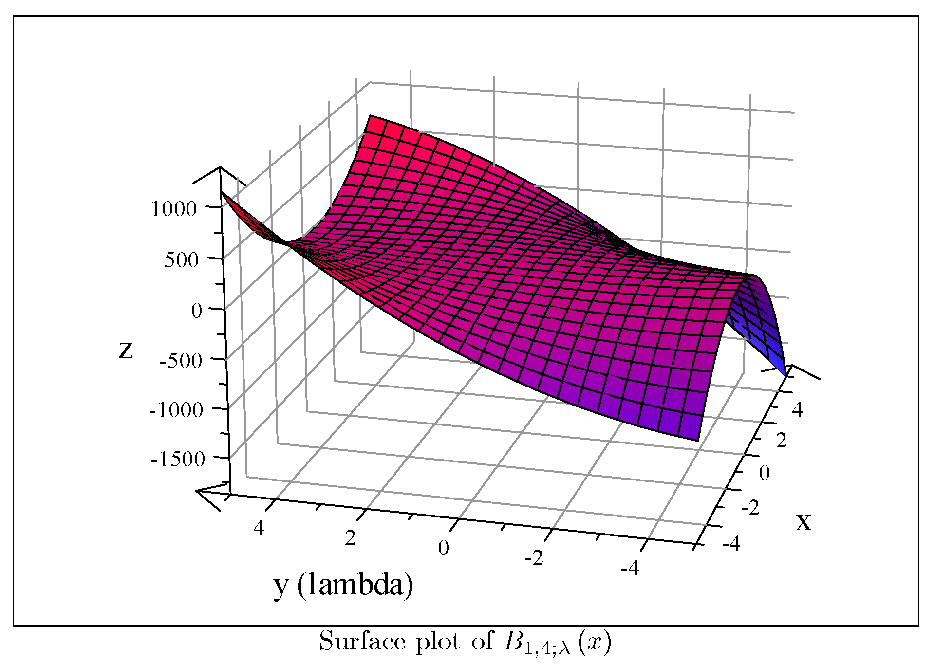
Upon setting $m=1$ in the Mac Laurin series expansions (57) and (58), we attain the first few $Detr$-Bernoulli numbers subsequently:

$$\begin{array}{c}{B}_{1,0;\lambda }=0,\\ B_{1,1;\lambda }=0,\\ B_{1,2;\lambda }=\frac{\lambda -1}{2},\\ B_{1,3;\lambda }=\frac{\lambda -1}{2},\\ B_{1,4;\lambda }=\frac{\lambda -1}{2}\left(1+\frac{{\left(1\right)}_{2,\lambda }}{2}\right),\\ B_{1,5;\lambda }=\frac{\lambda -1}{2}\left(1+{\left(1\right)}_{2,\lambda }+\frac{{\left(1\right)}_{3,\lambda }}{6}\right),\\ B_{1,6;\lambda }=\frac{\lambda -1}{2}\left(1+\frac{3{\left(1\right)}_{2,\lambda }}{2}+\frac{{\left(1\right)}_{3,\lambda }}{6}+\frac{{\left({\left(1\right)}_{2,\lambda }\right)}^2}{4}+\frac{{\left(1\right)}_{3,\lambda }{\left(1\right)}_{2,\lambda }}{12}+\frac{{\left(1\right)}_{4,\lambda }{\left(1\right)}_{2,\lambda }}{48}\right)\end{array}$$

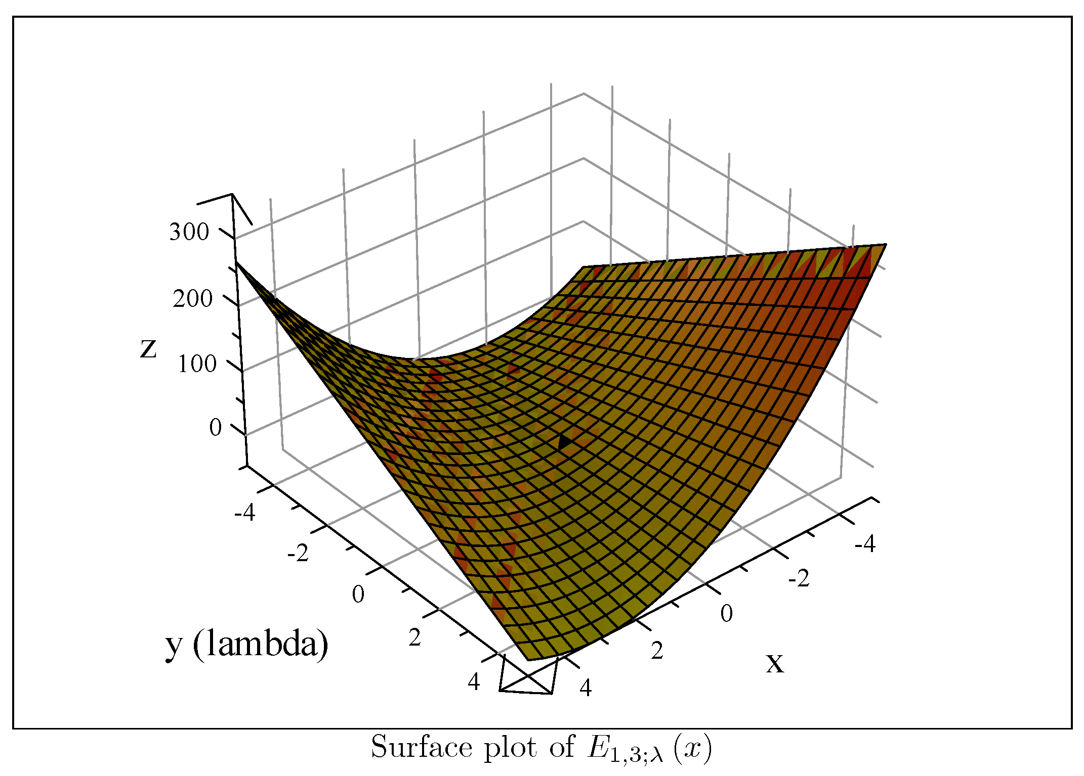
and we acquire the first few $Detr$-Euler numbers obviously:

$$\begin{array}{c}{E}_{1,0;\lambda }=0,\\ E_{1,1;\lambda }=2,\\ E_{1,2;\lambda }=-2,\\ E_{1,3;\lambda }=2-{\left(1\right)}_{2,\lambda },\\ E_{1,4;\lambda }=-2+2{\left(1\right)}_{2,\lambda }-\frac{{\left(1\right)}_{3,\lambda }}{3},\\ E_{1,5;\lambda }=2-3{\left(1\right)}_{2,\lambda }+\frac{{\left({\left(1\right)}_{2,\lambda }\right)}^2}{2}+\frac{2{\left(1\right)}_{3,\lambda }}{3}-\frac{{\left(1\right)}_{4,\lambda }}{12},\\ E_{1,6;\lambda }=-2+4{\left(1\right)}_{2,\lambda }-3\frac{{\left({\left(1\right)}_{2,\lambda }\right)}^2}{2}+\frac{{\left(1\right)}_{3,\lambda }{\left(1\right)}_{2,\lambda }}{3}-+{\left(1\right)}_{3,\lambda }+\frac{{\left(1\right)}_{4,\lambda }}{6}-\frac{{\left(1\right)}_{5,\lambda }}{60}.\end{array}$$

In conjunction with the computations performed above and via (59) and (60) (with $m=1$) given by

$$B_{1,n,\lambda }\left(x\right)=\sum _{k=0}^n\left(\genfrac{}{}{0pt}{}{n}{k}\right){\left(x\right)}_{k,\lambda }{B}_{1,n-k,\lambda }$$

and

$$E_{1,n,\lambda }\left(x\right)=\sum _{k=0}^n\left(\genfrac{}{}{0pt}{}{n}{k}\right){\left(x\right)}_{k,\lambda }{E}_{1,n-k,\lambda },$$

we can compute the first few $Detr$-Bernoulli polynomials:

$$\begin{array}{c}{B}_{1,0;\lambda }\left(x\right)=0,\\ B_{1,1;\lambda }\left(x\right)=0,\\ B_{1,2;\lambda }\left(x\right)=\frac{\lambda -1}{2},\\ B_{1,3;\lambda }\left(x\right)=\frac{\lambda -1}{2}\left(1+3x\right),\\ B_{1,4;\lambda }\left(x\right)=\frac{\lambda -1}{2}\left(1+\frac{{\left(1\right)}_{2,\lambda }}{2}+4x+12x^2+6{\left(x\right)}_{2,\lambda }\right),\\ B_{1,5;\lambda }\left(x\right)=\frac{\lambda -1}{2}\left(1+{\left(1\right)}_{2,\lambda }+\frac{{\left(1\right)}_{3,\lambda }}{6}+1+\frac{{\left(1\right)}_{2,\lambda }}{2}5x+10{\left(x\right)}_{2,\lambda }+10{\left(x\right)}_{3,\lambda }\right),\\ B_{1,6;\lambda }\left(x\right)=\frac{\lambda -1}{2}\left(1+\frac{3{\left(1\right)}_{2,\lambda }}{2}+\frac{{\left(1\right)}_{3,\lambda }}{6}+\frac{{\left({\left(1\right)}_{2,\lambda }\right)}^2}{4}+\frac{{\left(1\right)}_{3,\lambda }{\left(1\right)}_{2,\lambda }}{12}+\frac{{\left(1\right)}_{4,\lambda }{\left(1\right)}_{2,\lambda }}{48}\right)\\ +\frac{\lambda -1}{2}\left(\left(6+6{\left(1\right)}_{2,\lambda }+{\left(1\right)}_{3,\lambda }\right)x+15\left(1+\frac{{\left(1\right)}_{2,\lambda }}{2}\right){\left(x\right)}_{2,\lambda }+20{\left(x\right)}_{3,\lambda }+15{\left(x\right)}_{4,\lambda }\right)\end{array}$$

and we acquire the first few $Detr$-Euler polynomials subsequently:

$$\begin{array}{c}{E}_{1,0;\lambda }\left(x\right)=0,\\ E_{1,1;\lambda }\left(x\right)=2,\\ E_{1,2;\lambda }\left(x\right)=-2+4x,\\ E_{1,3;\lambda }\left(x\right)=2-{\left(1\right)}_{2,\lambda }-6x+6{\left(x\right)}_{2,\lambda },\\ E_{1,4;\lambda }\left(x\right)=-2+2{\left(1\right)}_{2,\lambda }-\frac{{\left(1\right)}_{3,\lambda }}{3}+\left(2-{\left(1\right)}_{2,\lambda }\right)4x-12{\left(x\right)}_{2,\lambda }+8{\left(x\right)}_{3,\lambda },\\ E_{1,5;\lambda }\left(x\right)=2-3{\left(1\right)}_{2,\lambda }+\frac{{\left({\left(1\right)}_{2,\lambda }\right)}^2}{2}+\frac{2{\left(1\right)}_{3,\lambda }}{3}-\frac{{\left(1\right)}_{4,\lambda }}{12}+\left(-2+2{\left(1\right)}_{2,\lambda }-\frac{{\left(1\right)}_{3,\lambda }}{3}\right)5x\\ +\left(2-{\left(1\right)}_{2,\lambda }\right)10{\left(x\right)}_{2,\lambda }-20{\left(x\right)}_{3,\lambda }+10{\left(x\right)}_{4,\lambda },\\ E_{1,6;\lambda }\left(x\right)=-2+4{\left(1\right)}_{2,\lambda }-3\frac{{\left({\left(1\right)}_{2,\lambda }\right)}^2}{2}+\frac{{\left(1\right)}_{3,\lambda }{\left(1\right)}_{2,\lambda }}{3}-+{\left(1\right)}_{3,\lambda }+\frac{{\left(1\right)}_{4,\lambda }}{6}-\frac{{\left(1\right)}_{5,\lambda }}{60}\\ +\left(2-3{\left(1\right)}_{2,\lambda }+\frac{{\left({\left(1\right)}_{2,\lambda }\right)}^2}{2}+\frac{2{\left(1\right)}_{3,\lambda }}{3}-\frac{{\left(1\right)}_{4,\lambda }}{12}\right)6x\\ +\left(-2+2{\left(1\right)}_{2,\lambda }-\frac{{\left(1\right)}_{3,\lambda }}{3}\right)15{\left(x\right)}_{2,\lambda }+\left(2-{\left(1\right)}_{2,\lambda }\right)20{\left(x\right)}_{3,\lambda }-30{\left(x\right)}_{4,\lambda }+12{\left(x\right)}_{5,\lambda }.\end{array}$$

The Detr-Bernoulli and the Detr-Euler polynomials have interesting surface plots in the special values. We would like to show the quirky surface plots of the $B_{1,4;\lambda }\left(x\right)$ and $E_{1,4;\lambda }\left(x\right)$ as given in Figure 3 and Figure 4.

6. The Degenerate Truncated Bell Polynomials

In this section, we perform to define and examine the degenerate truncated forms of the bivariate Bell polynomials and numbers. Then, we develop multifarious identities and correlations for these polynomials and numbers, which includes addition formulas, summation formulas, recurrence relationships, difference operator property and derivative rules. Moreover we provide diverse correlations and formulas related to the Apostol-type $Detr$-Stirling polynomials of the second kind and the $Detr$-Stirling polynomials of the second kind.

The classical Bell polynomials $Be{l}_n\left(x\right)$ (also called exponential polynomials) are defined by means of the following generating function ([3,4,19,24]):

$$\sum _{n=0}^{\infty }Be{l}_n\left(x\right)\frac{t^n}{n!}=e^{x\left(e^t-1\right)}.$$

(79)

The classical Bell numbers $Be{l}_n$ are attained by taking $x=1$ in (79), i.e., $Be{l}_n\left(1\right):=Be{l}_n$ and are given by the following exponential generating function ([3,4,19,24]):

$$\sum _{n=0}^{\infty }Be{l}_n\frac{t^n}{n!}=e^{\left(e^t-1\right)}.$$

(80)

The Bell polynomials introduced by Bell [3] appear as a standard mathematical tool and arise in combinatorial analysis. Since the first consideration of the Bell polynomials, these polynomials have been intensely investigated and studied by several mathematicians, [3,4,18,19,22,23,24,25] and see also the references cited therein.

The usual Bell polynomials and Stirling numbers of the second kind satisfy the following relation ([3,4,19,24])

$$Be{l}_n\left(x\right)=\sum _{m=0}^n{S}_2\left(n,m\right)x^m.$$

(81)

The degenerate Bell polynomials are given by the following Taylor series expansion at $t=0$ as follows ([18,22,23,25]):

$$\sum _{n=0}^{\infty }Be{l}_{n,\lambda }\left(x\right)\frac{t^n}{n!}=e^{x\left(e_{\lambda }\left(t\right)-1\right)}.$$

(82)

When $x=1$ in (82), the polynomials $Be{l}_{n,\lambda }\left(x\right)$ reduce to the degenerate Bell numbers $Be{l}_{n,\lambda }\left(1\right):=Be{l}_{n,\lambda }$ with the following generating function

$$\sum _{n=0}^{\infty }Be{l}_{n,\lambda }\frac{t^n}{n!}=e^{\left(e_{\lambda }\left(t\right)-1\right)}.$$

(83)

We note that the degenerate Bell polynomials (81) reduce the classical Bell polynomials (81) in the following limit case:

$$\underset{\lambda \to 0}{lim}Be{l}_{n,\lambda }\left(x\right)=Be{l}_n\left(x\right).$$

The degenerate Bell polynomials and the degenerate Stirling numbers of the second kind satisfy the following correlation ([18,22,23,25])

$$Be{l}_{n,\lambda }\left(x\right)=\sum _{m=0}^n{S}_{2,\lambda }\left(n,m\right)x^m.$$

(84)

Now, we are ready to introduce the bivariate degenerate truncated Bell polynomials, which we choose to call the $Detr$-Bell polynomials as given below.

Definition 5.

Let x be an independent variable and $m\in {\mathbb{N}}_0$. The bivariate degenerate truncated Bell polynomials $Be{l}_{m,n;\lambda }\left(x,y\right)$ are defined by the following exponential generating function:

$$\sum _{n=0}^{\infty }Be{l}_{m,n;\lambda }\left(x,y\right)\frac{t^n}{n!}=e^{y\left(e_{\lambda }\left(t\right)-1-e_{m-1,\lambda }\left(t\right)\right)}{e}_{\lambda }^x\left(t\right).$$

(85)

Upon setting $y=1$ and $x=0$ in (85), the bivariate truncated degenerate Bell polynomials reduce to the corresponding numbers $Be{l}_{m,n;\lambda }\left(0,1\right):=Be{l}_{m,n;\lambda }$ termed the degenerate truncated Bell numbers, which we call the $Detr$-Bell numbers:

$$\sum _{n=0}^{\infty }Be{l}_{m,n;\lambda }\frac{t^n}{n!}=e^{\left(e_{\lambda }\left(t\right)-1-e_{m-1,\lambda }\left(t\right)\right)}.$$

(86)

We now examine diverse special cases of the bivariate $Detr$-Bell polynomials as follows.

Remark 10.

1. 

When $x=0$ in (85), the polynomials $Be{l}_{m,n;\lambda }\left(x,y\right)$ in (85) reduce to the degenerate truncated Bell polynomials $Be{l}_{m,n;\lambda }\left(y\right)$ in (87), which are also new generalizations of the Bell polynomials $Be{l}_n\left(x\right)$ in (1), given by

$$\sum _{n=0}^{\infty }Be{l}_{m,n;\lambda }\left(y\right)\frac{t^n}{n!}=e^{y\left(e_{\lambda }\left(t\right)-1-e_{m-1,\lambda }\left(t\right)\right)}.$$

(87)

2. 

Upon setting $\lambda \to 0$ in (85), we get a new generalization of the usual Bell polynomials, which we call the bivariate truncated Bell polynomials $Be{l}_{m,n}\left(x,y\right)$ (88), shown by

$$\sum _{n=0}^{\infty }Be{l}_{m,n}\left(x,y\right)\frac{t^n}{n!}=e^{y\left(e^t-1-e_{m-1}\left(t\right)\right)}{e}^{xt}.$$

(88)

3. 

In the special case $\lambda \to 0$ and $x=0$, we acquire a novel extension of the Bell polynomials, which we call the truncated Bell polynomials $Be{l}_{m,n}\left(y\right)$ as follows

$$\sum _{n=0}^{\infty }Be{l}_{m,n;\lambda }\left(x,y\right)\frac{t^n}{n!}=e^{y\left(e^t-1-e_{m-1}\left(t\right)\right)}.$$

(89)

4. 

Choosing $m=0$ in (85), we obtain the bivariate degenerate Bell polynomials given below ([23]):

$$\sum _{n=0}^{\infty }Be{l}_{n;\lambda }\left(x,y\right)\frac{t^n}{n!}=e^{y\left(e_{\lambda }\left(t\right)-1\right)}{e}_{\lambda }^x\left(t\right).$$

(90)

5. 

Setting $m=x=0$ in (85), we attain the degenerate Bell polynomials in (82) ([18,22,23,25]).

6. 

When $\lambda \to m=x=0$ in (85), we arrive at the familiar Bell polynomials in (79) ([3,4,19,24]).

We now investigate some properties and formulas of the bivariate $Detr$-Bell polynomials $Be{l}_{m,n;\lambda }\left(x,y\right)$. Hence, we first provide the following theorem.

Theorem 25.

For $n,m\in {\mathbb{N}}_0,$ we have

$$Be{l}_{m,n;\lambda }\left(x,y\right)=\sum _{l=0}^n\left(\genfrac{}{}{0pt}{}{n}{l}\right)Be{l}_{m,l;\lambda }\left(y\right){\left(x\right)}_{n-l,\lambda }.$$

(91)

Proof. 

By means of (85) and (87), we get

$$\begin{array}{ccc}\hfill \sum _{n=0}^{\infty }Be{l}_{m,n;\lambda }\left(x,y\right)\frac{t^n}{n!}& =& e^{y\left(e_{\lambda }\left(t\right)-1-e_{m-1,\lambda }\left(t\right)\right)}{e}_{\lambda }^x\left(t\right)\hfill \\ & =& \sum _{n=0}^{\infty }Be{l}_{m,n;\lambda }\left(y\right)\frac{t^n}{n!}\sum _{n=0}^{\infty }{\left(x\right)}_{n,\lambda }\frac{t^n}{n!}\hfill \\ & =& \sum _{n=0}^{\infty }\sum _{l=0}^n\left(\genfrac{}{}{0pt}{}{n}{l}\right)Be{l}_{m,l;\lambda }\left(y\right){\left(x\right)}_{n-l,\lambda }\frac{t^n}{n!},\hfill \end{array}$$

which gives the asserted result (91). □

An extension of the well-known correlations in (81) and (84) is given below.

Theorem 26.

The following relation

$$Be{l}_{m,n;\lambda }\left(x,y\right)=\sum _{k=0}^n{y}^k{S}_{2,m;\lambda }\left(n,k:x\right)$$

(92)

holds true for $n,m\in {\mathbb{N}}_0$.

Proof. 

By the Definition 5 and the Formula (22), we get

$$\begin{array}{ccc}\hfill \sum _{n=0}^{\infty }Be{l}_{m,n;\lambda }\left(x,y\right)\frac{t^n}{n!}& =& \sum _{k=0}^{\infty }{y}^k\frac{{\left(e_{\lambda }\left(t\right)-1-e_{m-1,\lambda }\left(t\right)\right)}^k}{k!}{e}_{\lambda }^x\left(t\right)\hfill \\ & =& \sum _{k=0}^{\infty }{y}^k\sum _{n=0}^{\infty }{S}_{2,m;\lambda }\left(n,k:x\right)\frac{t^n}{n!}\hfill \\ & =& \sum _{n=0}^{\infty }\sum _{k=0}^n{y}^k{S}_{2,m;\lambda }\left(n,k:x\right)\frac{t^n}{n!},\hfill \end{array}$$

which gives the claimed result (92). □

We now provide an addition formula for $Be{l}_{m,n;\lambda }\left(x,y\right)$ as follows.

Theorem 27.

The following summation formula

$$Be{l}_{m,n;\lambda }\left(x_1+x_2,y_1+y_2\right)=\sum _{u=0}^n\left(\genfrac{}{}{0pt}{}{n}{u}\right)Be{l}_{m,n-u;\lambda }\left(x_1,y_1\right)Be{l}_{m,u;\lambda }\left(x_2,y_2\right),$$

(93)

is valid for $n,m\in {\mathbb{N}}_0$.

Proof. 

By Definition 5 and the identity (60), we obtain

$$\begin{array}{ccc}\hfill \sum _{n=0}^{\infty }Be{l}_{m,n;\lambda }\left(x_1+x_2,y_1+y_2\right)\frac{t^n}{n!}& =& e^{\left(y_1+y_2\right)\left(e_{\lambda }\left(t\right)-1-e_{m-1,\lambda }\left(t\right)\right)}{e}_{\lambda }^{x_1+x_2}\left(t\right)\hfill \\ & =& e^{y_1\left(e_{\lambda }\left(t\right)-1-e_{m-1,\lambda }\left(t\right)\right)}{e}_{\lambda }^{x_1}\left(t\right)e^{y_2\left(e_{\lambda }\left(t\right)-1-e_{m-1,\lambda }\left(t\right)\right)}{e}_{\lambda }^{x_2}\left(t\right)\hfill \\ & =& \sum _{n=0}^{\infty }Be{l}_{m,n;\lambda }\left(x_1,y_1\right)\frac{t^n}{n!}\sum _{n=0}^{\infty }Be{l}_{m,n;\lambda }\left(x_2,y_2\right)\frac{t^n}{n!}\hfill \\ & =& \sum _{n=0}^{\infty }\sum _{u=0}^n\left(\genfrac{}{}{0pt}{}{n}{u}\right)Be{l}_{m,n-u;\lambda }\left(x_1,y_1\right)Be{l}_{m,u;\lambda }\left(x_2,y_2\right)\frac{t^n}{n!},\hfill \end{array}$$

which provides the desired result (93). Henceforth, the proof is completed. □

Two immediate consequences of the Theorem 27 are discussed below.

Corollary 2.

For $n,m\in {\mathbb{N}}_0$, we have

$$Be{l}_{m,n;\lambda }\left(x,y_1+y_2\right)=\sum _{u=0}^n\left(\genfrac{}{}{0pt}{}{n}{u}\right)Be{l}_{m,n-u;\lambda }\left(x,y_1\right)Be{l}_{m,u;\lambda }\left(y_2\right)$$

and

$$Be{l}_{m,n;\lambda }\left(x_1+x_2,y\right)=\sum _{u=0}^n\left(\genfrac{}{}{0pt}{}{n}{u}\right)Be{l}_{m,n-u;\lambda }\left(x_1,y_1\right){\left(x_2\right)}_{u,\lambda }.$$

We now provide a correlation as follows.

Theorem 28.

The following formula

$$Be{l}_{m,n;\lambda }\left(x,y\right)=\sum _{u=0}^n\sum _{l=0}^n\left(\genfrac{}{}{0pt}{}{n}{u}\right)Be{l}_{m,u;\lambda }\left(y\right)S_{2;\lambda }\left(n-u,l:-l\right){\left(x\right)}^{\left(l\right)}$$

(94)

holds true for $n,m\in {\mathbb{N}}_0$.

Proof. 

By Definition 5 and Equation (26), we get

$$\begin{array}{ccc}\hfill \sum _{n=0}^{\infty }Be{l}_{m,n;\lambda }\left(x,y\right)\frac{t^n}{n!}& =& e^{y\left(e_{\lambda }\left(t\right)-1-e_{m-1,\lambda }\left(t\right)\right)}{\left(e_{\lambda }^{-1}\left(t\right)-1+1\right)}^x\hfill \\ & =& e^{y\left(e_{\lambda }\left(t\right)-1-e_{m-1,\lambda }\left(t\right)\right)}\sum _{l=0}^{\infty }\left(\genfrac{}{}{0pt}{}{x+l-1}{l}\right){\left(1-e_{\lambda }^{-1}\left(t\right)\right)}^l\hfill \\ & =& e^{y\left(e_{\lambda }\left(t\right)-1-e_{m-1,\lambda }\left(t\right)\right)}\sum _{l=0}^{\infty }\left(\genfrac{}{}{0pt}{}{x+l-1}{l}\right)\frac{{\left(e_{\lambda }\left(t\right)-1\right)}^l}{l!}{e}_{\lambda }^{-l}\left(t\right)l!\hfill \\ & =& \sum _{l=0}^{\infty }{\left(x\right)}^{\left(l\right)}\sum _{n=0}^{\infty }Be{l}_{m,n;\lambda }\left(y\right)\frac{t^n}{n!}\sum _{n=0}^{\infty }{S}_{2;\lambda }\left(n,l:-l\right)\frac{t^n}{n!}\hfill \\ & =& \sum _{l=0}^{\infty }{\left(x\right)}^{\left(l\right)}\sum _{n=0}^{\infty }\left(\sum _{u=0}^n\left(\genfrac{}{}{0pt}{}{n}{u}\right)Be{l}_{m,u;\lambda }\left(y\right)S_{2;\lambda }\left(n-u,l:-l\right)\right)\frac{t^n}{n!},\hfill \end{array}$$

which gives the claimed result (94). □

We now give a recurrence formula for $Be{l}_{m,n;\lambda }\left(x,y\right)$ as follows.

Theorem 29.

The following recurrence formula

$$Be{l}_{m,n;\lambda }\left(x,y\right)=n!\sum _{k=0}^{n-ml}\sum _{l=0}^k{y}^k\frac{{\left({\left(1\right)}_{m,\lambda }\right)}^l}{l!{\left(m!\right)}^l}\frac{S_{2,m;\lambda }\left(n-ml,k-l:x\right)}{\left(n-ml\right)!}$$

(95)

holds true for $n,m\in {\mathbb{N}}_0$.

Proof. 

In view of the Definition 5, we acquire

$$\begin{array}{ccc}\hfill \sum _{n=0}^{\infty }Be{l}_{m+1,n;\lambda }\left(x,y\right)\frac{t^n}{n!}& =& \sum _{k=0}^{\infty }{y}^k\frac{{\left(e_{\lambda }\left(t\right)-1-e_{m,\lambda }\left(t\right)\right)}^k}{k!}{e}_{\lambda }^x\left(t\right)\hfill \\ & =& \sum _{k=0}^{\infty }{y}^k\frac{{\left(e_{\lambda }\left(t\right)-1-e_{m-1,\lambda }\left(t\right)-{\left(1\right)}_{m,\lambda }\frac{t^m}{m!}\right)}^k}{k!}{e}_{\lambda }^x\left(t\right)\hfill \\ & =& \sum _{k=0}^{\infty }\frac{y^k}{k!}\sum _{l=0}^k\left(\genfrac{}{}{0pt}{}{k}{l}\right){\left(e_{\lambda }\left(t\right)-1-e_{m-1,\lambda }\left(t\right)\right)}^{k-l}{\left({\left(1\right)}_{m,\lambda }\right)}^l\frac{t^{ml}}{{\left(m!\right)}^l}{e}_{\lambda }^x\left(t\right)\hfill \\ & =& \sum _{k=0}^{\infty }{y}^k\sum _{l=0}^k\frac{{\left(e_{\lambda }\left(t\right)-1-e_{m-1,\lambda }\left(t\right)\right)}^{k-l}}{\left(k-l\right)!}{e}_{\lambda }^x\left(t\right){\left({\left(1\right)}_{m,\lambda }\right)}^l\frac{t^{ml}}{l!{\left(m!\right)}^l}\hfill \\ & =& \sum _{k=0}^{\infty }{y}^k\sum _{l=0}^k{\left({\left(1\right)}_{m,\lambda }\right)}^l\frac{t^{ml}}{l!{\left(m!\right)}^l}\sum _{n=0}^{\infty }{S}_{2,m;\lambda }\left(n,k-l:x\right)\frac{t^n}{n!}\hfill \\ & =& \sum _{n=0}^{\infty }\sum _{k=0}^n\sum _{l=0}^k{y}^k\frac{{\left({\left(1\right)}_{m,\lambda }\right)}^l}{l!{\left(m!\right)}^l}{S}_{2,m;\lambda }\left(n,k-l:x\right)\frac{t^{n+ml}}{n!}\hfill \end{array}$$

which gives the asserted result (95). □

We now give a formula for $Be{l}_{m,n;\lambda }\left(x,y\right)$ as follows.

Theorem 30.

The following operator formula

$${\mathsf{\Delta }}_{\lambda }Be{l}_{m,n;\lambda }\left(x,y\right)=nBe{l}_{m,n-1;\lambda }\left(x,y\right)$$

(96)

holds true for $n,m\in {\mathbb{N}}_0$.

Proof. 

In view of the Definition 5, by applying difference operator ${\mathsf{\Delta }}_{\lambda }$ (12) to both sides of Formula (96), we obtain

$$\begin{array}{ccc}\hfill \sum _{n=0}^{\infty }{\mathsf{\Delta }}_{\lambda }Be{l}_{m,n;\lambda }\left(x,y\right)\frac{t^n}{n!}& =& e^{y\left(e_{\lambda }\left(t\right)-1-e_{m-1,\lambda }\left(t\right)\right)}{\mathsf{\Delta }}_{\lambda }{e}_{\lambda }^x\left(t\right)\hfill \\ & =& e^{y\left(e_{\lambda }\left(t\right)-1-e_{m-1,\lambda }\left(t\right)\right)}{e}_{\lambda }^x\left(t\right)t\hfill \\ & =& \sum _{n=0}^{\infty }Be{l}_{m,n;\lambda }\left(x,y\right)\frac{t^{n+1}}{n!},\hfill \end{array}$$

which gives the assertion in (96). □

We now present the following derivation property with respect to x for the bivariate polynomials $Be{l}_{m,n;\lambda }\left(x,y\right)$.

Theorem 31.

The following formula

$$\frac{\partial }{\partial x}Be{l}_{m,n;\lambda }\left(x,y\right)=n!\sum _{l=1}^{\infty }Be{l}_{m,n-l;\lambda }\left(x,y\right)\frac{{\left(-1\right)}^{l+1}}{\left(n-l\right)!l}{\lambda }^{l-1}$$

(97)

holds true for $m,n\in {\mathbb{N}}_0$.

Proof. 

By applying derivative operator $\frac{\partial }{\partial x}$ with respect to x to both sides of Formula (85), we then derive

$$\begin{array}{ccc}\hfill \sum _{n=0}^{\infty }\frac{\partial }{\partial x}Be{l}_{m,n;\lambda }\left(x,y\right)\frac{t^n}{n!}& =& e^{y\left(e_{\lambda }\left(t\right)-1-e_{m-1,\lambda }\left(t\right)\right)}\frac{\partial }{\partial x}{\left(1+\lambda t\right)}^{\frac{x}{\lambda }}\hfill \\ & =& e^{y\left(e_{\lambda }\left(t\right)-1-e_{m-1,\lambda }\left(t\right)\right)}{\left(1+\lambda t\right)}^{\frac{x}{\lambda }}ln{\left(1+\lambda t\right)}^{\frac{1}{\lambda }}\hfill \\ & =& \sum _{n=0}^{\infty }Be{l}_{m,n;\lambda }\left(x,y\right)\frac{t^n}{n!}\sum _{u=1}^{\infty }\frac{{\left(-1\right)}^{u+1}}{u}{\lambda }^{u-1}{t}^u\hfill \\ & =& \sum _{n=0}^{\infty }\sum _{u=1}^{\infty }Be{l}_{m,n;\lambda }\left(x,y\right)\frac{{\left(-1\right)}^{u+1}}{u}{\lambda }^{u-1}\frac{t^{n+u}}{n!}\hfill \end{array}$$

which yields the asserted derivative Formula (97). □

Here is another derivation property for the bivariate polynomials $Be{l}_{m,n;\lambda }\left(x,y\right)$.

Theorem 32.

The following relation

$$\frac{\partial }{\partial y}Be{l}_{m,n;\lambda }\left(x,y\right)=\sum _{l=0}^{n-m}\frac{{\left(1\right)}_{l+m,\lambda }}{\left(l+m\right)!}Be{l}_{m,n-m-l;\lambda }\left(x,y\right)\frac{n!}{\left(n-l\right)!}-Be{l}_{m,n;\lambda }\left(x,y\right)$$

(98)

holds true for$m,n\in {\mathbb{N}}_0$.

Proof. 

By applying derivative operator with respect to y to both sides of the Formula (85), then we have

$$\sum _{n=0}^{\infty }Be{l}_{m,n;\lambda }\left(x,y\right)\frac{t^n}{n!}=e^{y\left(e_{\lambda }\left(t\right)-1-e_{m-1,\lambda }\left(t\right)\right)}{e}_{\lambda }^x\left(t\right).$$

$$\begin{array}{ccc}\hfill \sum _{n=0}^{\infty }\frac{\partial }{\partial y}Be{l}_{m,n;\lambda }\left(x,y\right)\frac{t^n}{n!}& =& \frac{\partial }{\partial y}{e}^{y\left(e_{\lambda }\left(t\right)-1-e_{m-1,\lambda }\left(t\right)\right)}{e}_{\lambda }^x\left(t\right)\hfill \\ & =& \left(e_{\lambda }\left(t\right)-1-e_{m-1,\lambda }\left(t\right)\right)e^{y\left(e_{\lambda }\left(t\right)-1-e_{m-1,\lambda }\left(t\right)\right)}{e}_{\lambda }^x\left(t\right)\hfill \\ & =& \left(\sum _{n=m}^{\infty }{\left(1\right)}_{n,\lambda }\frac{t^n}{n!}-1\right)e^{y\left(e_{\lambda }\left(t\right)-1-e_{m-1,\lambda }\left(t\right)\right)}{e}_{\lambda }^x\left(t\right)\hfill \\ & =& \sum _{n=0}^{\infty }{\left(1\right)}_{n+m,\lambda }\frac{t^{n+m}}{\left(n+m\right)!}\sum _{n=0}^{\infty }Be{l}_{m,n;\lambda }\left(x,y\right)\frac{t^n}{n!}-\sum _{n=0}^{\infty }Be{l}_{m,n;\lambda }\left(x,y\right)\frac{t^n}{n!}\hfill \\ & =& \sum _{n=0}^{\infty }\sum _{l=0}^n\frac{{\left(1\right)}_{l+m,\lambda }}{\left(l+m\right)!}Be{l}_{m,n-l;\lambda }\left(x,y\right)\frac{t^{n+m}}{\left(n-l\right)!}-\sum _{n=0}^{\infty }Be{l}_{m,n;\lambda }\left(x,y\right)\frac{t^n}{n!}\hfill \end{array}$$

which yields the asserted derivative Formula (98). □

7. Multifarious Connected Formulas

In this section, we first introduce the degenerate truncated Bernstein polynomials. We then perform to investigate diverse correlations and formulas including several polynomials such as the degenerate truncated Bernstein polynomials, the bivariate $Detr$-Fubini polynomials, the bivariate $Detr$-Bell polynomials, the $Detr$-Bernoulli polynomials, the $Detr$-Stirling polynomials of the second kind and the $Detr$-Euler polynomials.

For $x\in \left[0,1\right]$, the usual Bernstein polynomials ([1]) are given by the following generating function:

$$\sum _{n=0}^{\infty }{\mathfrak{B}}_{k,n}\left(x\right)\frac{t^n}{n!}=e^{\left(1-x\right)t}\frac{x^k}{k!}{t}^k.$$

(99)

The degenerate Bernstein polynomials ${\mathfrak{B}}_{k,n}\left(x:\lambda \right)$ for $x\in \left[0,1\right]$ are considered by Kim and Kim [20] by means of the following generating function to be

$$\sum _{n=0}^{\infty }{\mathfrak{B}}_{k,n}\left(x:\lambda \right)\frac{t^n}{n!}=e_{\lambda }^{1-x}\left(t\right)\frac{{\left(x\right)}_{k,\lambda }}{k!}{t}^k.$$

(100)

We first introduce the degenerate truncated Bernstein polynomials, which we call the $Detr$-Bernstein polynomials as follows.

Definition 6.

For $x\in \left[0,1\right]$ and $m\in {\mathbb{N}}_0$, the degenerate truncated Bernstein polynomials are defined by the following Mac Laurin series expansion at $t=0$:

$$\sum _{n=0}^{\infty }{\mathfrak{B}}_{k,n}^{\left[m\right]}\left(x:\lambda \right)\frac{t^n}{n!}={\left(e_{\lambda }\left(t\right)-e_{m-1,\lambda }\left(t\right)\right)}^{1-x}\frac{{\left(x\right)}_{k,\lambda }}{k!}{t}^k.$$

(101)

Remark 11.

In the limit case $\lambda \to 0$ in (101), we attain a new extension of the classical Bernstein polynomials ${\mathfrak{B}}_{k,n}\left(x\right)$, which we call the truncated Bernstein polynomials given by

$$\sum _{n=0}^{\infty }{\mathfrak{B}}_{k,n}^{\left[m\right]}\left(x\right)\frac{t^n}{n!}={\left(e^t-e_{m-1}\left(t\right)\right)}^{1-x}\frac{{\left(x\right)}^k}{k!}{t}^k.$$

(102)

Remark 12.

When $m=0$, the degenerate truncated Bernstein polynomials ${\mathfrak{B}}_{k,n}^{\left[m\right]}\left(x:\lambda \right)$ reduce to the degenerate Bernstein polynomials ${\mathfrak{B}}_{k,n}\left(x:\lambda \right)$ in (100).

We consider that

$$\begin{array}{ccc}\hfill \sum _{n=0}^{\infty }{\mathfrak{B}}_{k,n}^{\left[m\right]}\left(x:\lambda \right)\frac{t^n}{n!}& =& {\left(e_{\lambda }\left(t\right)-e_{m-1,\lambda }\left(t\right)\right)}^{1-x}\frac{{\left(x\right)}_{k,\lambda }}{k!}{t}^k\hfill \\ & =& {\left(e_{\lambda }\left(t\right)-1-e_{m-1,\lambda }\left(t\right)+1\right)}^{1-x}\frac{{\left(x\right)}_{k,\lambda }}{k!}{t}^k\hfill \\ & =& \sum _{l=0}^{\infty }{\left(1-x\right)}_l\frac{{\left(e_{\lambda }\left(t\right)-1-e_{m-1,\lambda }\left(t\right)\right)}^l}{l!}\frac{{\left(x\right)}_{k,\lambda }}{k!}{t}^k\hfill \\ & =& \sum _{l=0}^{\infty }{\left(1-x\right)}_l\sum _{n=0}^{\infty }{S}_{2,m;\lambda }\left(n,l:x\right)\frac{t^{n+k}}{n!}\frac{{\left(x\right)}_{k,\lambda }}{k!}\hfill \\ & =& \sum _{n=0}^{\infty }\sum _{l=0}^{\infty }{\left(1-x\right)}_l{S}_{2,m;\lambda }\left(n,l:x\right)\frac{{\left(x\right)}_{k,\lambda }}{k!}\frac{t^{n+k}}{n!}.\hfill \end{array}$$

Hence we arrive at the following theorem including a relation between the $Detr$-Bernstein polynomials and the $Detr$-Stirling polynomials of the second kind.

Theorem 33.

For $x\in \left[0,1\right]$, we have

$${\mathfrak{B}}_{k,n}^{\left[m\right]}\left(x:\lambda \right)=\sum _{l=0}^{n-k}\left(\genfrac{}{}{0pt}{}{n}{k}\right){\left(x\right)}_{k,\lambda }{\left(1-x\right)}_l{S}_{2,m;\lambda }\left(n-k,l:x\right).$$

(103)

By using (106) and (62) in conjunction with (79), we consider that

$$\begin{array}{c}\sum _{n=0}^{\infty }Be{l}_{m,n;\lambda }\left(x,y\right)\frac{t^n}{n!}=\sum _{k=0}^{\infty }{y}^k\frac{{\left(e_{\lambda }\left(t\right)-1-e_{m-1,\lambda }\left(t\right)\right)}^k}{k!}{e}_{\lambda }^x\left(t\right)\\ =\sum _{k=0}^{\infty }{y}^k\frac{{\left(e_{\lambda }\left(t\right)-e_{m-1,\lambda }\left(t\right)-1\right)}^k}{k!}{e}_{\lambda }^x\left(t\right)\\ =\sum _{k=0}^{\infty }\frac{y^k}{k!}{e}_{\lambda }^x\left(t\right)\sum _{l=0}^k\left(\genfrac{}{}{0pt}{}{k}{l}\right){\left(-1\right)}^{k-l}{\left(e_{\lambda }\left(t\right)-e_{m-1,\lambda }\left(t\right)\right)}^l\frac{{\left(1-l\right)}_{k,\lambda }}{k!}{t}^k\frac{k!}{{\left(1-l\right)}_{k,\lambda }}{t}^{-k}\\ =\sum _{k=0}^{\infty }{y}^k\sum _{l=0}^k\left(\genfrac{}{}{0pt}{}{k}{l}\right)\frac{{\left(-1\right)}^{k-l}}{{\left(1-l\right)}_{k,\lambda }}{t}^{-k}\sum _{n=0}^{\infty }{\left(x\right)}_{n,\lambda }\frac{t^n}{n!}\sum _{n=0}^{\infty }{\mathfrak{B}}_{k,n}^{\left[m\right]}\left(1-l:\lambda \right)\frac{t^n}{n!}\\ =\sum _{k=0}^{\infty }{y}^k\sum _{l=0}^k\left(\genfrac{}{}{0pt}{}{k}{l}\right)\frac{{\left(-1\right)}^{k-l}}{{\left(1-l\right)}_{k,\lambda }}\sum _{n=0}^{\infty }\sum _{u=0}^n\left(\genfrac{}{}{0pt}{}{n}{u}\right){\left(x\right)}_{n-u,\lambda }{\mathfrak{B}}_{k,u}^{\left[m\right]}\left(1-l:\lambda \right)\frac{t^{n-k}}{n!}\end{array}$$

Thus, we obtain the following theorem including a correlation covering the $Detr$-Bernstein polynomials and the $Detr$-Bell polynomials.

Theorem 34.

The following correlation

$$Be{l}_{m,n;\lambda }\left(x,y\right)=n!\sum _{k=0}^n\sum _{l=0}^k\sum _{u=0}^{n-k}{y}^k\left(\genfrac{}{}{0pt}{}{k}{l}\right)\frac{{\left(-1\right)}^{k-l}}{{\left(1-l\right)}_{k,\lambda }}\frac{{\left(x\right)}_{n-k-u,\lambda }}{\left(n-k-u\right)!u!}{\mathfrak{B}}_{k,u}^{\left[m\right]}\left(1-l:\lambda \right)$$

(104)

In terms of (74) and (85), we see that

$$\begin{array}{c}\sum _{n=0}^{\infty }Be{l}_{m,n;\lambda }\left(x,y\right)\frac{t^n}{n!}=e^{y\left(e_{\lambda }\left(t\right)-1-e_{m-1,\lambda }\left(t\right)\right)}{e}_{\lambda }^x\left(t\right)\\ =\sum _{l=0}^{\infty }{y}^l\frac{{\left(e_{\lambda }\left(t\right)-1-e_{m-1,\lambda }\left(t\right)\right)}^l}{l!}{e}_{\lambda }^x\left(t\right)\\ =\sum _{l=0}^{\infty }\frac{y^l}{l!}{\left(\frac{e_{\lambda }\left(t\right)-1-e_{m-1,\lambda }\left(t\right)}{{\left(1\right)}_{m+1,\lambda }\frac{t^{m+1}}{\left(m+1\right)!}}\right)}^l{e}_{\lambda }^x\left(t\right){\left({\left(1\right)}_{m+1,\lambda }\right)}^l\frac{t^{\left(m+1\right)l}}{{\left(\left(m+1\right)!\right)}^l}\\ =\sum _{l=0}^{\infty }\frac{y^l}{l!}\frac{{\left({\left(1\right)}_{m+1,\lambda }\right)}^l}{{\left(\left(m+1\right)!\right)}^l}\sum _{n=0}^{\infty }{B}_{m,n,\lambda }^{\left(-l\right)}\left(x\right)\frac{t^{n+\left(m+1\right)l}}{n!}.\end{array}$$

Thus, we arrive at the following theorem including the bivariate $Detr$-Bell polynomials and the $Detr$-Bernoulli polynomials.

Theorem 35.

The following summation equality

$$Be{l}_{m,n;\lambda }\left(x,y\right)=n!\sum _{l=0}^{\infty }\frac{y^l}{l!}\frac{{\left({\left(1\right)}_{m+1,\lambda }\right)}^l}{{\left(\left(m+1\right)!\right)}^l}\frac{B_{m,n-\left(m+1\right),\lambda }^{\left(-l\right)}\left(x\right)}{\left(n-\left(m+1\right)\right)!}$$

(105)

is valid.

By means of (37) and (56)

$$\begin{array}{ccc}\hfill \sum _{n=0}^{\infty }{F}_{m,n;\lambda }\left(x,-\frac{1}{2}\right)\frac{t^n}{n!}& =& \frac{{\left(1\right)}_{m,\lambda }\frac{t^m}{m!}{e}_{\lambda }^x\left(t\right)}{1+\frac{1}{2}\left(e_{\lambda }\left(t\right)-1-e_{m-1,\lambda }\left(t\right)\right)}\hfill \\ & =& \frac{2{\left(1\right)}_{m,\lambda }\frac{t^m}{m!}{e}_{\lambda }^x\left(t\right)}{e_{\lambda }\left(t\right)+1-e_{m-1,\lambda }\left(t\right)}\hfill \\ & =& \sum _{n=0}^{\infty }{E}_{m,n,\lambda }\left(x\right)\frac{t^n}{n!}.\hfill \end{array}$$

Therefore, we obtain the following theorem involving the bivariate $Detr$-Fubini polynomials and the $Detr$-Euler polynomials.

Theorem 36.

The following relation

$$F_{m,n;\lambda }\left(x,-\frac{1}{2}\right)=E_{m,n,\lambda }\left(x\right)$$

(106)

holds true for $m,n\in {\mathbb{N}}_0$.

An immediate result for Formula (106) is as follows.

Corollary 3.

Setting $x=0$ in (106), we then get a relation between the $Detr$-Fubini polynomials and the $Detr$-Euler numbers:

$$F_{m,n;\lambda }\left(-\frac{1}{2}\right)=E_{m,n;\lambda }.$$

(107)

Remark 13.

The relationships (106) and (107) are extensions of the well-known relation given by ([15])

$$F_n\left(-\frac{1}{2}\right)=E_n.$$

By (37) and (56), we get

$$\begin{array}{c}\sum _{n=0}^{\infty }{F}_{m,n;\lambda }\left(x,y\right)\frac{t^n}{n!}=\frac{{\left(1\right)}_{m,\lambda }\frac{t^m}{m!}{e}_{\lambda }^x\left(t\right)}{1-y\left(e_{\lambda }\left(t\right)-1-e_{m-1,\lambda }\left(t\right)\right)}\frac{2\frac{t^m}{m!}{\left(1\right)}_{m,\lambda }}{e_{\lambda }\left(t\right)+1-e_{m-1,\lambda }\left(t\right)}\frac{e_{\lambda }\left(t\right)+1-e_{m-1,\lambda }\left(t\right)}{2\frac{t^m}{m!}{\left(1\right)}_{m,\lambda }}\\ =\frac{1}{2{\left(1\right)}_{m,\lambda }}\frac{m!}{t^m}\sum _{n=0}^{\infty }{F}_{m,n;\lambda }\left(y\right)\frac{t^n}{n!}\sum _{n=0}^{\infty }{E}_{m,n;\lambda }\left(x\right)\frac{t^n}{n!}\left(\sum _{n=m}^{\infty }{\left(1\right)}_{n,\lambda }\frac{t^n}{n!}+1\right)\\ =\frac{m!}{2{\left(1\right)}_{m,\lambda }}\sum _{n=0}^{\infty }\left(\sum _{l=0}^n\left(\genfrac{}{}{0pt}{}{n}{l}\right)F_{m,l;\lambda }\left(y\right)E_{m,n-l;\lambda }\left(x\right)\right)\frac{t^{n-m}}{n!}\left(\sum _{j=0}^{\infty }{\left(1\right)}_{n+m,\lambda }\frac{t^{n+m}}{\left(n+m\right)!}+1\right)\\ =\frac{m!}{2{\left(1\right)}_{m,\lambda }}\sum _{n=0}^{\infty }\left(\sum _{l=0}^n\left(\genfrac{}{}{0pt}{}{n}{l}\right)F_{m,l;\lambda }\left(y\right)E_{m,n-l;\lambda }\left(x\right)\right)\frac{t^{n-m}}{n!}\\ +\frac{m!}{2{\left(1\right)}_{m,\lambda }}\sum _{n=0}^{\infty }\sum _{j=0}^n\left(\genfrac{}{}{0pt}{}{n+m}{j}\right){\left(1\right)}_{n+m-j,\lambda }\left(\sum _{l=0}^j\left(\genfrac{}{}{0pt}{}{j}{l}\right)F_{m,l;\lambda }\left(y\right)E_{m,j-l;\lambda }\left(x\right)\right)\frac{t^n}{\left(n+m\right)!}.\end{array}$$

Hence, we state the following theorem which includes a correlation for the $F_{m,n;\lambda }\left(x,y\right)$, $F_{m,n;\lambda }\left(y\right)$ and $E_{m,n;\lambda }\left(x\right)$.

Theorem 37.

The following relation

$$\begin{array}{ccc}\hfill F_{m,n;\lambda }\left(x,y\right)& =& \frac{n!m!}{\left(n+m\right)!}\sum _{l=0}^{n+m}\frac{1}{2{\left(1\right)}_{m,\lambda }}\left(\genfrac{}{}{0pt}{}{n+m}{l}\right)F_{m,l;\lambda }\left(y\right)E_{m,n+m-l;\lambda }\left(x\right)\hfill \\ & & +\frac{n!m!}{\left(n+m\right)!}\sum _{j=0}^n\frac{1}{2{\left(1\right)}_{m,\lambda }}\left(\genfrac{}{}{0pt}{}{n+m}{j}\right)F_{m,l;\lambda }\left(y\right)E_{m,j-l;\lambda }\left(x\right)\hfill \end{array}$$

(108)

is valid for $n,m\in {\mathbb{N}}_0$.

By using the generating functions of the $Detr$-Bernoulli and the bivariate $Detr$-Fubini polynomials in (37) and (55), we derive

$$\begin{array}{ccc}\hfill \sum _{n=0}^{\infty }{F}_{m,n;\lambda }\left(x,y\right)\frac{t^n}{n!}& =& \frac{{\left(1\right)}_{m,\lambda }\frac{t^m}{m!}{e}_{\lambda }^x\left(t\right)}{1-y\left(e_{\lambda }\left(t\right)-1-e_{m-1,\lambda }\left(t\right)\right)}\frac{{\left(1\right)}_{m+1,\lambda }\frac{t^{m+1}}{\left(m+1\right)!}}{e_{\lambda }\left(t\right)-1-e_{m-1,\lambda }\left(t\right)}\frac{e_{\lambda }\left(t\right)-1-e_{m-1,\lambda }\left(t\right)}{{\left(1\right)}_{m+1,\lambda }\frac{t^{m+1}}{\left(m+1\right)!}}\hfill \\ & =& \frac{\left(m+1\right)!}{{\left(1\right)}_{m+1,\lambda }{t}^{m+1}}\sum _{n=0}^{\infty }{F}_{m,n;\lambda }\left(x,y\right)\frac{t^n}{n!}\sum _{n=0}^{\infty }{B}_{m,n,\lambda }\left(x\right)\frac{t^n}{n!}\left(\sum _{n=m}^{\infty }{\left(1\right)}_{n,\lambda }\frac{t^n}{n!}-1\right)\hfill \\ & =& \frac{\left(m+1\right)!}{{\left(1\right)}_{m+1,\lambda }}\sum _{n=0}^{\infty }\left(\sum _{k=0}^n\left(\genfrac{}{}{0pt}{}{n}{k}\right)F_{m,k;\lambda }\left(y\right)B_{m,n-k;\lambda }\left(x\right)\right)\frac{t^n}{n!}\sum _{n=0}^{\infty }{\left(1\right)}_{n+m,\lambda }\frac{t^{n-1}}{\left(n+m\right)!}\hfill \\ & & -\sum _{n=0}^{\infty }\frac{\left(m+1\right)!}{{\left(1\right)}_{m+1,\lambda }}\left(\sum _{k=0}^n\left(\genfrac{}{}{0pt}{}{n}{k}\right)F_{m,k;\lambda }\left(y\right)B_{m,n-k;\lambda }\left(x\right)\right)\frac{t^{n-m-1}}{n!}\hfill \\ & =& \frac{\left(m+1\right)!}{{\left(1\right)}_{m+1,\lambda }}\sum _{n=0}^{\infty }\left[\sum _{l=0}^n\left(\genfrac{}{}{0pt}{}{n+m}{l}\right)\left(\sum _{k=0}^l\left(\genfrac{}{}{0pt}{}{l}{k}\right)F_{m,k;\lambda }\left(y\right)B_{m,l-k;\lambda }\left(x\right)\right){\left(1\right)}_{n+m-l,\lambda }\right]\frac{t^{n-1}}{\left(n+m\right)!}\hfill \\ & & -\sum _{n=0}^{\infty }\frac{\left(m+1\right)!}{{\left(1\right)}_{m+1,\lambda }}\left(\sum _{k=0}^n\left(\genfrac{}{}{0pt}{}{n}{k}\right)F_{m,k;\lambda }\left(y\right)B_{m,n-k;\lambda }\left(x\right)\right)\frac{t^{n-m-1}}{n!}.\hfill \end{array}$$

Thus, we arrive at the following theorem.

Theorem 38.

The following relation

$$\begin{array}{ccc}\hfill F_{m,n;\lambda }\left(x,y\right)& =& \frac{n!\left(m+1\right)!}{{\left(1\right)}_{m+1,\lambda }}\sum _{l=0}^{n+1}\left(\genfrac{}{}{0pt}{}{n+m+1}{l}\right)\left(\sum _{k=0}^l\left(\genfrac{}{}{0pt}{}{l}{k}\right)F_{m,k;\lambda }\left(y\right)B_{m,l-k;\lambda }\left(x\right)\right){\left(1\right)}_{n+m+1-l,\lambda }\hfill \\ & & -\frac{n!\left(m+1\right)!}{{\left(1\right)}_{m+1,\lambda }}\left(\sum _{k=0}^{n+m+1}\left(\genfrac{}{}{0pt}{}{n+m+1}{k}\right)F_{m,k;\lambda }\left(y\right)B_{m,n+m+1-k;\lambda }\left(x\right)\right)\hfill \end{array}$$

(109)

is valid for non-negative integers m and n.

8. Conclusions

In the present paper, we have considered the degenerate truncated forms of the various special polynomials and numbers and have investigated their several properties and relationships by using the series manipulation method and some special proof techniques indicated in the proof of each of the theorem stated in this paper. We have first introduced the degenerate truncated exponential polynomials and have given their several properties. Then we have defined the degenerate truncated Stirling polynomials of the second kind and have proved their elementary properties and relations. We have also considered the degenerate truncated bivariate Fubini and Bell polynomials and numbers and we then have attained multifarious relations and formulas, which covers several summation formulas, addition identities, recurrence relationships, derivative property and correlations with the degenerate truncated Stirling polynomials of the second kind. Moreover, we have defined the truncated degenerate Bernoulli and Euler polynomials and have provided multifarious correlations and interesting formulas including summation formulas, derivation rules and correlations with the degenerate truncated Stirling numbers of the second. Furthermore, regarding applications, by introducing the degenerate truncated forms of the classical Bernstein polynomials, we have derived several correlations and formulas including the degenerate truncated Bernstein polynomials, the bivariate $Detr$-Fubini polynomials, the bivariate $Detr$-Bell polynomials, the $Detr$-Bernoulli polynomials, the $Detr$-Stirling polynomials of the second kind and the $Detr$-Euler polynomials. We have also provided several interesting surface plots of the aforementioned polynomials in the special cases. The results obtained in this paper are generalizations of the many earlier results, some of which are involved related references in [1,2,3,4,5,6,7,8,9,10,11,12,13,14,15,16,17,18,19,20,21,22,23,24,25,26,27,28,29,30,31,32,33,34,35,36,37]. For future directions, we will analyze that the polynomials introduced in this paper can be applied in the theory of umbral calculus and those can be connected with some degenerate probability distributions.

References

- Acikgoz, M.; Araci, S. On the generating function for Bernstein polynomials. In Proceedings of the AIP Conference Proceedings, Chonburi, Thailand, 18–20 July 2010; Volume 1281, p. 1141. [Google Scholar]
- Apostol, T.M. On the Lerch zeta function. Pac. J. Math. 1951, 1, 161–167. [Google Scholar]
- Bell, E.T. Exponential polynomials. Ann. Math. 1934, 35, 258–277. [Google Scholar] [CrossRef]
- Carlitz, L. Some remarks on the Bell numbers. Fibonacci Quart. 1980, 18, 66–73. [Google Scholar]
- Carlitz, L. Degenerate Stirling, Bernoulli and Eulerian numbers. Utilitas Math. 1975, 15, 51–88. [Google Scholar]
- Cheon, G.-S. A note on the Bernoulli and Euler polynomials. Appl. Math. Lett. 2003, 16, 365–368. [Google Scholar] [CrossRef] [Green Version]
- Choi, J.; Anderson, P.J.; Srivastava, H.M. Some q-extensions of the Apostol-Bernoulli and the Apostol-Euler polynomials of order n, and the multiple Hurwitz zeta function. Appl. Math. Comput. 2008, 199, 723–737. [Google Scholar] [CrossRef]
- Dattoli, G.; Ceserano, C.; Sacchetti, D. A note on truncated polynomials. Appl. Math. Comput. 2003, 134, 595–605. [Google Scholar] [CrossRef]
- Duran, U.; Acikgoz, M. Truncated Fubini polynomials. Mathematics 2019, 7, 431. [Google Scholar] [CrossRef] [Green Version]
- Duran, U.; Acikgoz, M. On some degenerate probability distributions related to the degenerate Stirling numbers of the second kind. 2019; in review. [Google Scholar]
- Duran, U.; Sadjang, P.N. On Gould-Hopper-based fully degenerate poly-Bernoulli polynomials with a q-parameter. Mathematics 2019, 7, 121. [Google Scholar] [CrossRef] [Green Version]
- Edwards, H.M. Riemann’s Zeta Function; Academic Press: New York, NY, USA, 1974; ISBN 0-12-232750-0. [Google Scholar]
- Hassen, A.; Nguyen, H.D. Hypergeometric Bernoulli polynomials and Appell sequences. Int. J. Number Theory 2008, 4, 767–774. [Google Scholar] [CrossRef] [Green Version]
- Howard, F.T. Explicit formulas for degenerate Bernoulli numbers. Discrete Math. 1996, 162, 175–185. [Google Scholar] [CrossRef] [Green Version]
- Kargın, L. Some formulae for products of Fubini polynomials with applications. arXiv 2016, arXiv:1701.01023v1. [Google Scholar]
- Kim, D.S.; Kim, T.; Kwon, H.-I.; Park, J.-W. Two variable higher-order Fubini polynomials. J. Korean Math. Soc. 2018, 55, 975–986. [Google Scholar] [CrossRef]
- Kim, T.; Kim, D.S.; Jang, G.-W. A note on degenerate Fubini polynomials. Proc. Jangjeon Math Soc. 2017, 20, 521–531. [Google Scholar]
- Kim, T.; Kim, D.S.; Jang, L.-C.; Kwon, H.I. Extended degenerate stirling numbers of the second kind and extended degenerate Bell polynomials. Utilitas Math. 2018, 106, 11–21. [Google Scholar]
- Kim, D.S.; Kim, T. Some identities of Bell polynomials. Sci. China Math. 2015, 58, 2095–2104. [Google Scholar] [CrossRef]
- Kim, T.; Kim, D.S. Degenerate Bernstein polynomials. RASCAM 2018. [Google Scholar] [CrossRef] [Green Version]
- Kim, T.; Kim, D.S.; Kim, H.Y.; Kwon, J. Degenerate Stirling polynomials of the second kind and some applications. Symmetry 2019, 11, 1046. [Google Scholar] [CrossRef] [Green Version]
- Kim, T.; Kim, D.S. On degenerate Bell numbers and polynomials. RASCAM 2017, 111, 435–446. [Google Scholar] [CrossRef]
- Kim, T.; Yao, Y.; Kim, D.S.; Jang, G.-W. Degenerate r-Stirling numbers and r-Bell polynomials. Russ. J. Math. Phys. 2018, 25, 44–58. [Google Scholar] [CrossRef]
- Kim, T.; Kim, D.S.; Jang, G.-W. Extended Stirling polynomials of the second kind and extended Bell polynomials. Proc. Jangjeon Math. Soc. 2017, 20, 365–376. [Google Scholar]
- Kim, T.; Kim, D.S.; Dolgy, D.V. On partially degenerate Bell numbers and polynomials. Proc. Jangjeon Math. Soc. 2017, 20, 337–345. [Google Scholar]
- Kim, T. A note on degenerate Stirling polynomials of the second kind. Proc. Jangjeon Math. Soc. 2017, 20, 319–331. [Google Scholar]
- Komatsu, T.; Ruiz, C.D.J.P. Truncated Euler polynomials. Math. Slovaca 2018, 68, 527–536. [Google Scholar] [CrossRef] [Green Version]
- Luo, Q.-M.; Srivastava, H.M. Some generalizations of the Apostol-Genocchi polynomials and the Stirling numbers of the second kind. Appl. Math. Comput. 2011, 217, 5702–5728. [Google Scholar] [CrossRef]
- Luo, Q.-M.; Srivastava, H.M. Some generalizations of the Apostol-Bernoulli and Apostol-Euler polynomials. J. Math. Anal. Appl. 2005, 308, 290–302. [Google Scholar] [CrossRef]
- Mihoubi, M. Bell polynomials and binomial type sequences. Discret. Math. 2008, 308, 2450–2459. [Google Scholar] [CrossRef] [Green Version]
- Kurt, B. Some relationships between the generalized Apostol-Bernoulli and Apostol-Euler polynomials. Turkish J. Anal. Number Theory 2013, 1, 54–58. [Google Scholar] [CrossRef]
- Kurt, B. Explicit relations for the modified degenerate Apostol-type polynomials. J. BAUN Inst. Sci. Technol. 2018, 20, 401–412. [Google Scholar]
- Srivastava, H.M.; Araci, S.; Khan, W.A.; Acikgoz, M. A note on the truncated-exponential based Apostol-type polynomials. Symmetry 2019, 11, 538. [Google Scholar] [CrossRef] [Green Version]
- Srivastava, H.M.; Choi, J. Zeta and q-Zeta Functions and Associated Series and Integrals; Elsevier Science Publishers: Amsterdam, The Netherlands, 2012; 674p. [Google Scholar]
- Srivastava, H.M.; Pinter, A. Remarks on some relationships between the Bernoulli and Euler polynomials. Appl. Math. Lett. 2004, 17, 375–380. [Google Scholar] [CrossRef] [Green Version]
- Su, D.D.; He, Y. Some identities for the two variable Fubini polynomials. Mathematics 2019, 7, 115. [Google Scholar] [CrossRef] [Green Version]
- Shank, Y. False positive and false negative effects on network attacks. J. Stat. Phys. 2018, 170, 141–164. [Google Scholar] [CrossRef]
Figure 1.
Surface Plot of .
Figure 2.
Figure 3.
Surface plot of .
Figure 4.
© 2020 by the authors. Licensee MDPI, Basel, Switzerland. This article is an open access article distributed under the terms and conditions of the Creative Commons Attribution (CC BY) license (http://creativecommons.org/licenses/by/4.0/).
Share and Cite
MDPI and ACS Style
Duran, U.; Acikgoz, M. On Degenerate Truncated Special Polynomials. Mathematics 2020, 8, 144. https://0-doi-org.brum.beds.ac.uk/10.3390/math8010144
AMA Style
Duran U, Acikgoz M. On Degenerate Truncated Special Polynomials. Mathematics. 2020; 8(1):144. https://0-doi-org.brum.beds.ac.uk/10.3390/math8010144
Chicago/Turabian StyleDuran, Ugur, and Mehmet Acikgoz. 2020. "On Degenerate Truncated Special Polynomials" Mathematics 8, no. 1: 144. https://0-doi-org.brum.beds.ac.uk/10.3390/math8010144
Note that from the first issue of 2016, this journal uses article numbers instead of page numbers. See further details here.