Online Batch Scheduling of Simple Linear Deteriorating Jobs with Incompatible Families

Abstract

We considered the online scheduling problem of simple linear deteriorating job families on m parallel batch machines to minimize the makespan, where the batch capacity is unbounded. In this paper, simple linear deteriorating jobs mean that the actual processing time $p_j$ of job $J_j$ is assumed to be a linear function of its starting time $s_j$, i.e., $p_j={\alpha }_j{s}_j$, where ${\alpha }_j>0$ is the deterioration rate. Job families mean that one job must belong to some job family, and jobs of different families cannot be processed in the same batch. When $m=1$, we provide the best possible online algorithm with the competitive ratio of ${(1+{\alpha }_{max})}^f$, where f is the number of job families and ${\alpha }_{max}$ is the maximum deterioration rate of all jobs. When $m\ge 1$ and $m=f$, we provide the best possible online algorithm with the competitive ratio of $1+{\alpha }_{max}$.

1. Introduction

1.1. Background

In this paper, all jobs arrive over time, i.e., each job has an arrival time. Before the jobs arrive, we do not know any information, including arrival time, processing time, deterioration rate, etc. Due to the unknown information of the jobs, the online algorithm is not guaranteed to be optimal. Borodin and El-Yaniv [1] used the competitive ratio to measure the quality of an online algorithm. For a minimization scheduling problem, we define the competitive ratio of the online algorithm A as:

$$\rho =sup\{A(\mathcal{I})/OPT(\mathcal{I}):\mathcal{I}\mathrm{is}\mathrm{any}\mathrm{instance}\mathrm{such}\mathrm{that}OPT(\mathcal{I})>0\}.$$

where $\mathcal{I}$ is any job instance and $A(\mathcal{I})$ and $OPT(\mathcal{I})$ are the objective values obtained from the algorithm A and an optimal offline scheduling $OPT$, respectively. In this study, the objective was to minimize the makespan. An online algorithm A is called the best possible if no other online algorithms $A^{*}$ produce a smaller competitive ratio.

Parallel-batch means that one batch processing machine can process b jobs simultaneously as a batch. The processing time of a batch is the maximum processing time of all jobs in this batch. All jobs in a batch have the same starting time, processing time, and completion time. According to the number of jobs contained in a batch, Brucker et al. [2] divided the model into two cases: the unbounded model $(b=\infty )$ and the bounded model $(b<\infty )$.

Job families mean that one job must belong to some job family, and jobs of different families cannot be processed in the same batch. Online scheduling problems on parallel batch machines with incompatible job families have been studied extensively. Fu et al. [3] studied the online algorithm on a single machine to minimize the makespan. Li et al. [4] examined the online scheduling of incompatible unit-length job families with lookahead on a single machine. Tian et al. [5] analyzed the problem on m parallel machines. However, research is lacking on the parallel-batch online scheduling with incompatible deteriorating job families.

Traditional scheduling problems assume that the processing time of a job is fixed. However, in real life, one job will take longer when it has a later starting time. For example, in steel production and financial management [6,7], the processing time is longer when it starts later. In the steel-making process, strict requirements are placed on temperature. If the waiting time is too long, the temperature of molten steel will drop. So, it will take time to heat up again before further processing. Other examples are provided in cleaning and fire fighting. The scheduling problem of deteriorating jobs was first introduced by Browne and Yechiali [8] and Gupta and Gupta [9], independently. Both considered minimizing makespan on a single machine. Since then, this topic has attracted considerable attentions. Gawiejnowicz and Kononov [10] considered the general properties of scheduling with fixed job processing time and scheduling with job processing time as proportional linear functions of the job starting time. The relevant research includes [11,12,13,14,15,16,17,18], among many others. Recently, some works have been published about online algorithms for linear deteriorating jobs [19,20,21,22,23].

To minimize the makespan of the online scheduling problem on m parallel machines with linear deteriorating jobs, Cheng et al. [19] constructed an algorithm and proved that the bound of the competitive ratio of the algorithm is tight, where $m=2$ and the largest deterioration rate of jobs is known in advance. Yu et al. [22] proved that no deterministic online algorithm is better than $(1+{\alpha }_{max})$-competitive when $m=2$, where ${\alpha }_{max}$ is the maximum deterioration rate of all jobs.

1.2. Research Problem

Our contribution is to extend the online scheduling problem on m parallel batch machines with simple linear deteriorating job families to minimize the makespan. Here, batch capacity is unbounded, i.e., $b=\infty$. We use f-family to denote there are f job families. We constructed the best possible online algorithm with the competitive ratio of ${(1+{\alpha }_{max})}^f$ when $m=1$, where f is the number of job families and ${\alpha }_{max}$ is the maximum deterioration rate of all jobs. When $m\ge 1$ and $m=f$, we created the best possible online algorithm with the competitive ratio of $1+{\alpha }_{max}$.

We examined the online batch scheduling of simple linear deteriorating job families. The actual processing time $p_j$ of job $J_j$ is assumed to be a linear function of its starting time $s_j$, i.e., $p_j={\alpha }_j{s}_j$, where ${\alpha }_j>0$ is the deterioration rate, which is unknown until it arrives. The objective was to minimize makespan. Assume that the arrival time of all jobs is greater than or equal to $t_0>0$; otherwise, jobs arriving at time 0 can be completed at time 0. We used the three-field notation $\alpha \left|\beta \right|\gamma$ [24] to represent one scheduling problem.

This paper is organized as follows. In Section 2, we consider the problem $1|\mathrm{online}$,$r_j$,$\mathrm{p}-\mathrm{batch},b=\infty$,f-family,$p_j={\alpha }_{j}t$$|C_{max}$, where f is the number of job families. We prove the lower bound and provide the best possible online algorithm with the competitive ratio of ${(1+{\alpha }_{max})}^f$. In Section 3, we consider the problem $Pm|\mathrm{online}$,$r_j$,$\mathrm{p}-\mathrm{batch},b=\infty$,m-family,$p_j={\alpha }_{j}t$$|C_{max}$, where m is the number of machines. We prove the lower bound and provide the best possible online algorithm with the competitive ratio of $1+{\alpha }_{max}$, where ${\alpha }_{max}$ is the maximum deterioration rate of all jobs.

Throughout this paper, we use $\sigma$ and $\pi$ to denote the schedules obtained from an online algorithm and an optimal offline schedule, respectively. Let $C_{max}(\sigma )$ and $C_{max}(\pi )$ be the objective values of $\sigma$ and $\pi$, respectively, and ${\alpha }_{max}$ be the maximum deterioration rate of all jobs. Let $ϵ$ be an arbitrary small positive number.

2. Single Batch Machine ($\mathit{m}=\mathbf{1}$)

In this section, we consider the online scheduling on an unbounded batch machine and the jobs belong to f incompatible deteriorating job families. The number of job families, f, is known in advance. We prove the lower bound and provide the best possible online algorithm with the competitive ratio of ${(1+{\alpha }_{max})}^f$.

Theorem 1.

For problem $1|online$,$r_j$,$p-batch,b=\infty$,f-family,$p_j={\alpha }_{j}t$$|C_{max}$, the competitive ratio of any online algorithm is not less than ${(1+{\alpha }_{max})}^f$.

Proof. 

Let H be any online algorithm and I be a job instance provided by the adversary. In instance I, all the jobs have the same deterioration rate of $\alpha$.

At time $t_0$, f jobs from the f different job families arrive by the adversary. If a job is scheduled by H to process at time t and t is in the time interval $[t_0,{(1+\alpha )}^f{t}_0)$, then at time $t+ϵ$, the adversary releases a copy of this job, which belongs to the same job family. Let s be the starting time of the first job whose completion time is at least ${(1+\alpha )}^f{t}_0$. $(1+\alpha )s\ge {(1+\alpha )}^f{t}_0$. so,

$$s\ge {(1+\alpha )}^{f-1}{t}_0.$$

(1)

Case 1${(1+\alpha )}^{f-1}{t}_0\le s<{(1+\alpha )}^f{t}_0$.

In this case, there are still f jobs from f distinct job families that are not processed at time $(1+\alpha )s$. So,

$$C_{max}(\sigma )\ge {(1+\alpha )}^f(1+\alpha )s={(1+\alpha )}^{f+1}s.$$

(2)

We assume that the jobs processed in the time interval $[t_0,(1+\alpha )s)$ belong to k distinct job families, say, ${\mathcal{F}}_1,{\mathcal{F}}_2,\cdots ,{\mathcal{F}}_k$, where $1\le k\le f$. The other $f-k$ job families are defined by ${\mathcal{F}}_{k+1},{\mathcal{F}}_{k+2},\cdots ,{\mathcal{F}}_f$. Let $s_i$ be the last starting time of the jobs in ${\mathcal{F}}_i$ that start before or at time s for $1\le i\le k$, and satisfy $s_1<s_2<\cdots <s_k$. Clearly, $s_k=s$. From the construction of instance I, we know that the last arrival time of the jobs in ${\mathcal{F}}_i$ $(1\le i\le k)$ is $s_i+ϵ$ and the arrival time of the jobs in ${\mathcal{F}}_i$ $(k+1\le i\le f)$ is $t_0$.

Construct a schedule ${\pi }^{\prime }$ below: the jobs in ${\mathcal{F}}_i$ $(1\le i\le f)$ form a batch starting at time ${s_i}^{\prime }$, where:

$${s_i}^{\prime }=\left\{\begin{array}{cc}{(1+\alpha )}^{i-(k+1)}{t}_0,\hfill & \hfill k+1\le i\le f\\ max\{s_i+ϵ,{(1+\alpha )}^{(f+i)-(k+1)}{t}_0\},\hfill & \hfill 1\le i\le k.\end{array}\right.$$

We can see that ${\pi }^{\prime }$ is feasible, and the maximum completion time of the jobs in ${\pi }^{\prime }$ is the completion time of the jobs in ${\mathcal{F}}_k$. So,

$$C_{max}({\pi }^{\prime })=(1+\alpha )max\{s_k+ϵ,{(1+\alpha )}^{f-1}{t}_0\}.$$

(3)

Since $s_k=s$, we have $C_{max}({\pi }^{\prime })=max\{(1+\alpha )(s+ϵ),{(1+\alpha )}^f{t}_0\}.$ and $C_{max}(\pi )\le C_{max}({\pi }^{\prime })$.

If $C_{max}({\pi }^{\prime })=(1+\alpha )(s+ϵ)$, then by Equation (2) we know that:

$$\begin{array}{c}\hfill \frac{C_{max}(\sigma )}{C_{max}(\pi )}\ge \frac{{(1+\alpha )}^{f+1}s}{(1+\alpha )(s+ϵ)}\to {(1+\alpha )}^f={(1+{\alpha }_{max})}^f,ϵ\to 0.\end{array}$$

If $C_{max}({\pi }^{\prime })={(1+\alpha )}^f{t}_0$, then by Equations (1) and (2), we know that:

$$\begin{array}{c}\hfill \frac{C_{max}(\sigma )}{C_{max}(\pi )}\ge \frac{{(1+\alpha )}^{f+1}s}{{(1+\alpha )}^f{t}_0}=\frac{(1+\alpha )s}{t_0}\ge {(1+\alpha )}^f={(1+{\alpha }_{max})}^f.\end{array}$$

Case 2$s\ge {(1+\alpha )}^f{t}_0$.

According to the constructing of I, $s_k$ is the last starting time of the jobs in time interval $[t_0,{(1+\alpha )}^f{t}_0)$, and $s_k+ϵ$ is the last arrival time of all jobs.

Since s is the starting time of the first job whose completion time is at least ${(1+\alpha )}^f{t}_0$, we obtain $(1+\alpha )s_k<{(1+\alpha )}^f{t}_0$, i.e., $s_k<{(1+\alpha )}^{f-1}{t}_0$. From Equation (3), we have:

$$\begin{array}{ccc}\hfill C_{max}({\pi }^{\prime })& =& max\{(1+\alpha )(s_k+ϵ),{(1+\alpha )}^f{t}_0\}\hfill \\ & \to & max\{(1+\alpha )s_k,{(1+\alpha )}^f{t}_0\}\hfill \\ & =& {(1+\alpha )}^f{t}_0,\hfill \end{array}$$

as $ϵ\to 0$.

By the definition of s, f jobs from f distinct job families have not been processed at time s. So,

$$\begin{array}{c}\hfill C_{max}(\sigma )\ge {(1+\alpha )}^{f}s.\end{array}$$

Thus,

$$\begin{array}{c}\hfill \frac{C_{max}(\sigma )}{C_{max}(\pi )}\ge \frac{{(1+\alpha )}^{f}s}{{(1+\alpha )}^f{t}_0}=\frac{s}{t_0}\ge {(1+\alpha )}^f={(1+{\alpha }_{max})}^f.\end{array}$$

The result follows. □

Before introducing the online algorithm, given a batch B, we define some notations in the following:

$J(B)$: the last job with maximum deterioration rate in B.

$r(B)$: the arrival time of $J(B)$.

$s(B)$: the starting time of $J(B)$ in $\sigma$.

$\alpha (B)$: the deterioration rate of $J(B)$.

$U(t)$: the set of the unprocessed jobs at time t.

$B_i(t)$: the set of the unprocessed jobs of the same family at time t, $1\le i\le f$, which is a waiting batch at time t if $B_i(t)\ne \varnothing$.

$\mathcal{B}(t)$: the set of the waiting batches at time t.

$|\mathcal{B}(t)|$: the number of all waiting batches at time t.

$r(\mathcal{B}(t))=min\{r(B):B\in \mathcal{B}(t)\}$.

The online algorithm, called $A_1$ (Algorithm 1), can be stated as follows. Without causing confusion, assume that $B_i(t)=B_i$ in the following.

Algorithm 1:$A_1$

Input: Job instance I. do

Step 0: Set $t=t_0$.

Step 1: If $\mathcal{B}(t)=\varnothing$, then go to Step 5.

Step 2: Let $\mathcal{B}(t)=\{B_1,B_2,\cdots ,B_k\}$ such that $\alpha (B_1)\ge \alpha (B_2)\ge \cdots \ge \alpha (B_k)$, where $k\le f$.

Step 3: If $t\ge {(1+\alpha (B_1))}^k{t}_0$, then process the batch $B_1$ at time t. Reset $t=(1+\alpha (B_1))t$. Return to Step 1.

Step 4: If $t<{(1+\alpha (B_1))}^k{t}_0$, then reset $t=min\{{(1+\alpha (B_1))}^k{t}_0,t^{*}\}$, where $t^{*}$ is the arrival time of the next job. Go to Step 2.

Step 5: If new jobs arrive after t, then reset t as the arrival time of the first new job. Go to Step 1.

Output: Job schedule $\sigma$.

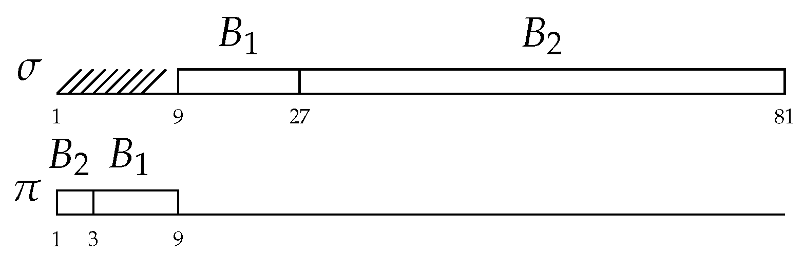
Example 1.

To make the algorithm more intuitive, we present an instance ${\mathcal{I}}_1$ in

Table 1. Instance ${\mathcal{I}}_1$.

Job	Arrival Time	Deterioration Rate
$J_1\in {\mathcal{F}}_1$	$r_1=t_0=1$	2
$J_2\in {\mathcal{F}}_2$	$r_2=t_0=1$	2
$J_3\in {\mathcal{F}}_1$	$r_3=2$	1

, where ${\mathcal{F}}_1$ and ${\mathcal{F}}_2$ are two different families. As shown in Figure 1, σ is the schedule generated by $A_1$ and π is an optimal offline schedule for ${\mathcal{I}}_1$, where $B_1=\{J_1,J_3\}$ and $B_2=\{J_2\}$.

We have $C_{max}(\sigma )=81$ and $C_{max}(\pi )=9$.

Suppose that $r_l$ is the last arrival time. Let $s\ge r_l$ be the minimum time, such that s is the starting time of some batch and there is no idle time between s and $C_{max}(\sigma )$ in $\sigma$. Let $\mathcal{B}$ be the set of the batches that process between s and $C_{max}(\sigma )$ in $\sigma$ and $s(\mathcal{B})$ be the start time of $\mathcal{B}$. Since $s(\mathcal{B})=s\ge r_l$, each batch in $\mathcal{B}$ is from a different family and $\mathcal{B}=\mathcal{B}(s)$. From Algorithm 1, $\mathcal{B}=\{B_1,B_2,\cdots ,B_k\}$ with $\alpha (B_1)\ge \alpha (B_2)\ge \cdots \ge \alpha (B_k)$, where $k\le f$. Then,

$$C_{max}(\sigma )=\prod _{i=1}^k(1+\alpha (B_i))s(\mathcal{B}).$$

(4)

The following two lemmas are the competition ratio analyses of Algorithm 1.

Lemma 1.

Suppose the machine has an idle time immediately before $s(\mathcal{B})$ in σ. Then, $C_{max}(\sigma )/C_{max}(\pi )\le {(1+{\alpha }_{max})}^f$.

Proof. 

Since an idle time occurs immediately before $s(\mathcal{B})$ in $\sigma$, from Algorithm 1, we have: $s(\mathcal{B})=max\{r_l,{(1+\alpha (B_1))}^k{t}_0\}$.

If $s(\mathcal{B})=r_l$, then for each $B_i\in \mathcal{B}$ with $1\le i\le k$, $J(B_i)$ arrives at time $r_l$. From Equation (4), we know that $C_{max}(\sigma )={\prod }_{i=1}^k(1+\alpha (B_i))r_l\le C_{max}(\pi ).$

If $s(\mathcal{B})={(1+\alpha (B_1))}^k{t}_0$, then from Equation (4) we have $C_{max}(\sigma )={\prod }_{i=1}^k(1+\alpha (B_i)){(1+\alpha (B_1))}^k{t}_0$. Since $C_{max}(\pi )\ge {\prod }_{i=1}^k(1+\alpha (B_i))t_0$, so $C_{max}(\sigma )/C_{max}(\pi )\le {(1+\alpha (B_1))}^k\le {(1+{\alpha }_{max})}^f$. □

Lemma 2.

Suppose the machine has no idle time immediately before $s(\mathcal{B})$ in σ. Then, $C_{max}(\sigma )/C_{max}(\pi )\le {(1+{\alpha }_{max})}^f$.

Proof. 

Since the machine has no idle time immediately before $s(\mathcal{B})$ in $\sigma$, $s(\mathcal{B})$ is the completion time of some batch, say $B^{*}$, in $\sigma$. We have $s(\mathcal{B})=(1+\alpha (B^{*}))s(B^{*})$. From the definition of s, we know $s(B^{*})<r_l$.

We suppose that $\mathcal{B}$ is divided into two sets, ${\mathcal{B}}_1$ and ${\mathcal{B}}_2$, such that:

$$\begin{array}{c}\hfill {\mathcal{B}}_1=\{B_i\in \mathcal{B}:r(B_i)>s(B^{*})\},\\ \hfill {\mathcal{B}}_2=\{B_j\in \mathcal{B}:r(B_j)\le s(B^{*})\}.\end{array}$$

Since $\mathcal{B}={\mathcal{B}}_1\bigcup {\mathcal{B}}_2$, $s(\mathcal{B})=(1+\alpha (B^{*}))s(B^{*})$, then from Equation (4) we have:

$$\begin{array}{ccc}\hfill C_{max}(\sigma )& =& \prod _{i=1}^k(1+\alpha (B_i))s(\mathcal{B})\hfill \\ & =& \prod _{B_i\in \mathcal{B}}(1+\alpha (B_i))s(\mathcal{B})\hfill \\ & =& \prod _{B_i\in {\mathcal{B}}_1}(1+\alpha (B_i))\prod _{B_j\in {\mathcal{B}}_2}(1+\alpha (B_j))(1+\alpha (B^{*}))s(B^{*}).\hfill \end{array}$$

From the definition of ${\mathcal{B}}_1$, we know $C_{max}(\pi )\ge {\prod }_{B_i\in {\mathcal{B}}_1}(1+\alpha (B_i))s(B^{*})$. Hence,

$$\begin{array}{ccc}\hfill C_{max}(\sigma )& =& \prod _{B_i\in {\mathcal{B}}_1}(1+\alpha (B_i))\prod _{B_j\in {\mathcal{B}}_2}(1+\alpha (B_j))(1+\alpha (B^{*}))s(B^{*})\hfill \\ & \le & \prod _{B_j\in {\mathcal{B}}_2}(1+\alpha (B_j))(1+\alpha (B^{*}))C_{max}(\pi ).\hfill \end{array}$$

According to the definition of ${\mathcal{B}}_2$ and Algorithm 1, each batch in set ${\mathcal{B}}_2$ and $B^{*}$ belongs to the different family. Then, at most $f-1$ batches exist in ${\mathcal{B}}_2$. Hence,

$$\begin{array}{c}\hfill C_{max}(\sigma )/C_{max}(\pi )\le \prod _{B_j\in {\mathcal{B}}_2}(1+\alpha (B_j))(1+\alpha (B^{*}))\le {(1+{\alpha }_{max})}^f.\end{array}$$

□

By Lemmas 1 and 2, and Theorem 1, we can reach the final conclusion.

Theorem 2.

For problem $1|online$,$r_j$,$p-batch,b=\infty$,f-family,$p_j={\alpha }_{j}t$$|C_{max}$, Algorithm 1 has a competitive ratio of ${(1+{\alpha }_{max})}^f$ and is the best possible.

3. Parallel Batch Machines ($\mathit{m}\ge \mathbf{1}$)

In this section, we consider the online scheduling on m parallel batch machines and the jobs belong to m incompatible deteriorating job families. We prove the lower bound and construct the best possible online algorithm with a competitive ratio of $1+{\alpha }_{max}$.

Theorem 3.

For problem $Pm|online$,$r_j$,$p-batch,b=\infty$,m-family,$p_j={\alpha }_{j}t$$|C_{max}$, no online algorithm exists with a competitive ratio less than $1+{\alpha }_{max}$.

Proof. 

Let H be any online algorithm and I be a job instance provided by the adversary. In the instance I, all the jobs have a deterioration rate of $\alpha$.

At time $t_0$, m jobs $J_1,J_2,\cdots ,J_m$ from different families arrive. Suppose that job $J_j$ starts processing at time $s_j$ in $\sigma$, $j=1,2,\cdots ,m$.

If a job $J_k$ exists such that $s_k\ge (1+\alpha )t_0$, where $1\le k\le m$, then the adversary does not release other jobs. Hence,

$$C_{max}(\sigma )\ge (1+\alpha )s_k\ge {(1+\alpha )}^2{t}_0\mathrm{and}{C}_{max}(\pi )=(1+\alpha )t_0.$$

We have $C_{max}(\sigma )/C_{max}(\pi )\ge 1+\alpha =1+{\alpha }_{max}$.

If for each job $J_j$ with $1\le j\le m$, $s_j<(1+\alpha )t_0$, let $J_l\in \{J_1,J_2,\cdots ,J_m\}$ is the last starting job. At time $s_l+ϵ$, a copy of the job $J_j(j=1,2,\cdots ,m)$ arrives. We have:

$$C_{max}(\sigma )\ge {(1+\alpha )}^2{s}_l\mathrm{and}{C}_{max}(\pi )=(1+\alpha )(s_l+ϵ).$$

Hence, $C_{max}(\sigma )/C_{max}(\pi )\ge (1+\alpha )s_l/(s_l+ϵ)\to 1+\alpha =1+{\alpha }_{max}$, as $ϵ\to 0$.

The result follows. □

Before providing the online algorithm, we define some notations used in the following:

$U(t)$: the set of the unprocessed jobs at time t.

${\alpha }_{max}(t)$: the maximum deterioration rate of the jobs arrived at t or before t.

$m(t)$: the number of the idle machines at time t.

$f(t)$: the number of job families in $U(t)$ at time t.

$B_i(t)$: the nonempty set of the unprocessed jobs of the same family at time t, where $1\le i\le f(t)$.

$J^i(t)$: the job with the maximum deterioration rate in $B_i(t)$, where $1\le i\le f(t)$.

${\alpha }^i(t)$: the deterioration rate of the job $J^i(t)$, where $1\le i\le f(t)$.

Without loss of generality, assume that ${\alpha }^1(t)\ge {\alpha }^2(t)\ge \cdots \ge {\alpha }^{f(t)}(t)$. The online algorithm, called $A_2$ (Algorithm 2), can be stated as follows.

Algorithm 2:$A_2$

Input: Job instance I. do

Step 0: Set $t=t_0$.

Step 1: If $U(t)=\varnothing$, then go to Step 6.

Step 2: If $m(t)=m$, and $t\ge (1+{\alpha }_{max}(t))t_0$, then at time t, start $B_i(t)$ as a single batch on the idle machine for any $i=1,2,\cdots ,f(t)$. Reset $t=(1+{\alpha }^{f(t)}(t))t$. Go to Step 1.

Step 3: If $m(t)=m$, and $t<(1+{\alpha }_{max}(t))t_0$, then reset $t=t^{*}$, such that $t^{*}$ is either the arrival time of the next job or $(1+{\alpha }_{max}(t))t_0$. Go to Step 1.

Step 4: If $m(t)<m$, and $t\ge (1+{\alpha }_{max}(t))(1+{\alpha }^1(t))t_0$, then at time t, start $B_i(t)$ as a single batch on the idle machine for any $i=1,2,\cdots ,min\{m(t),f(t)\}$. Reset $t=t^{*}$, such that $t^{*}$ is either the arrival time of the next job or $(1+{\alpha }^{min\{m(t),f(t)\}}(t))t$. Go to Step 1.

STEP 5: If $m(t)<m$, and $t<(1+{\alpha }_{max}(t))(1+{\alpha }^1(t))t_0$, then reset $t=t^{*}$, such that either $t^{*}$ is the arrival time of the next job or $m(t^{*})>m(t)$, or $t^{*}=(1+{\alpha }_{max}(t))(1+{\alpha }^1(t))t_0$.

Step 6: If new jobs arrive after t, then reset t as the arrival time of the first new job. Go to Step 1.

Output: Job schedule $\sigma$.

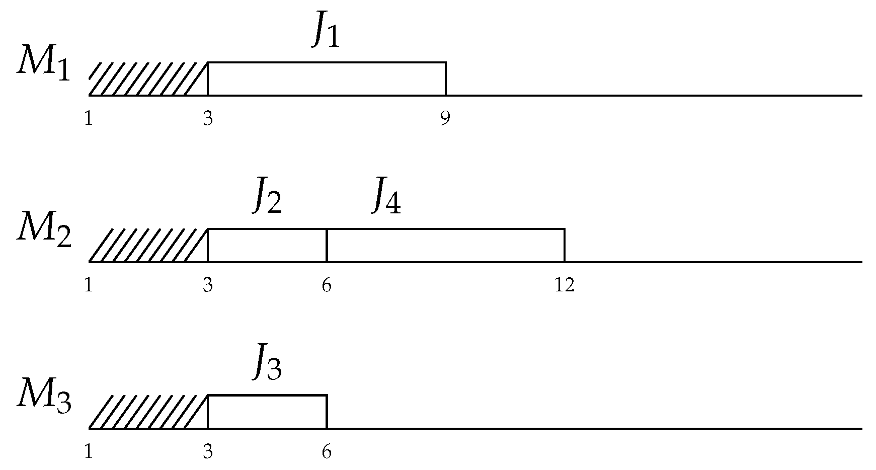
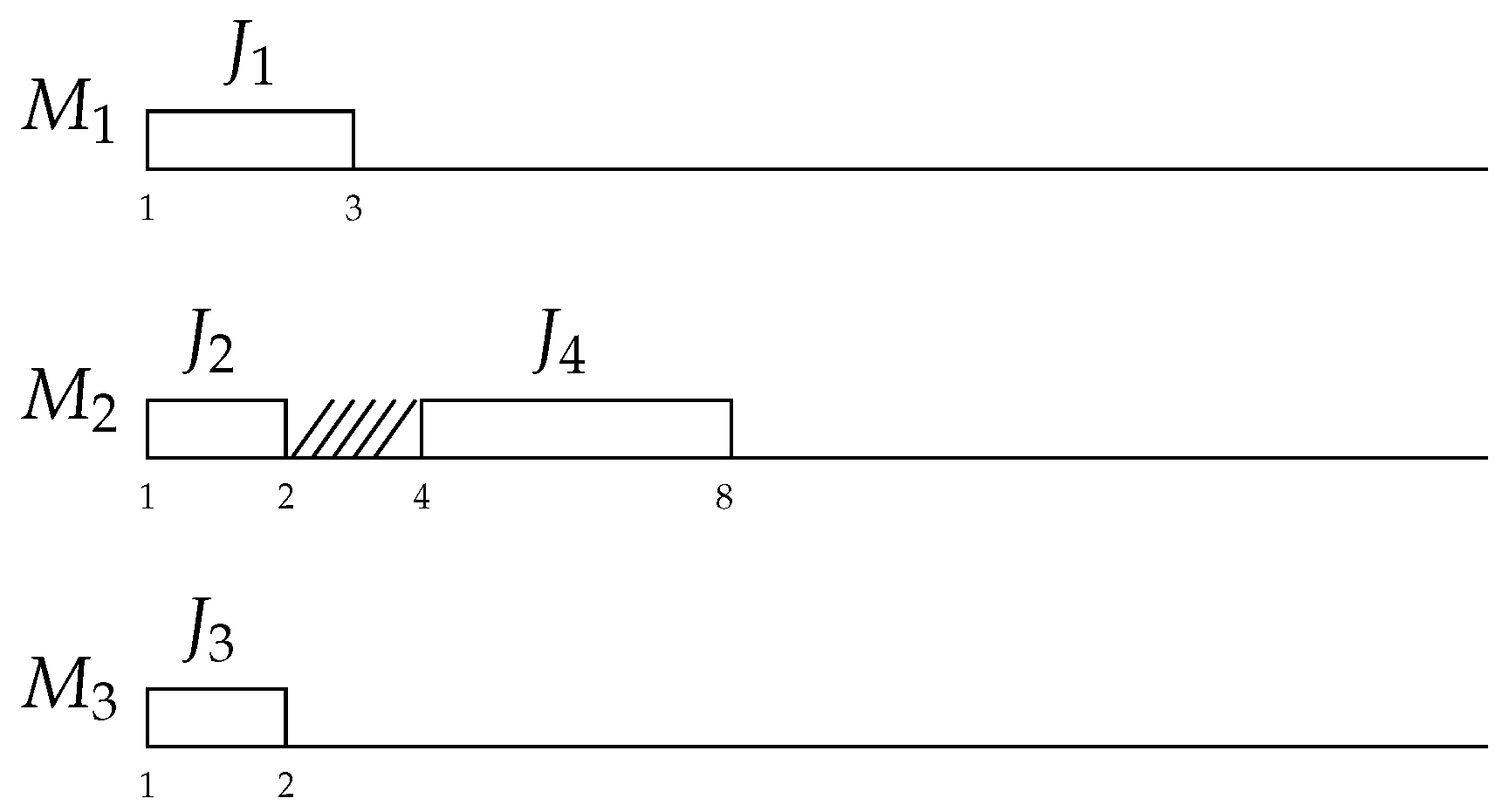
Example 2.

To make the algorithm more intuitive, we present an instance ${\mathcal{I}}_2$ in

Table 2. Instance ${\mathcal{I}}_2$.

Job	Arrival Time	Deterioration Rate
$J_1\in {\mathcal{F}}_1$	$r_1=t_0=1$	2
$J_2\in {\mathcal{F}}_2$	$r_2=t_0=1$	1
$J_3\in {\mathcal{F}}_3$	$r_3=t_0=1$	1
$J_4\in {\mathcal{F}}_1$	$r_4=4$	1

. Figure 2 depicts the schedule generated by Algorithm 2 and Figure 3 is an optimal offline schedule for ${\mathcal{I}}_2$.

We have $C_{max}(\sigma )=12$ and $C_{max}(\pi )=8$.

Suppose that Algorithm 2 generates n batches $B_1,B_2,\cdots B_n$. For batch $B_i$, we define some notations in the following:

$J_i$: the job with the maximum deterioration rate in $B_i$.

${\alpha }_i$: the deterioration rate of $J_i$ or the deterioration rate of $B_i$.

$r_i$: the arrival time of $J_i$.

$s_i$: the starting time of $B_i$ in $\sigma$, suppose that $s_1\le s_2\le \cdots \le s_n$.

The following is the competition ratio analysis of the Algorithm 2.

Let $B_l$ be the first batch in $\sigma$ assuming the objective value. $B_i$ is a regular batch if $s_i=max\{(1+{\alpha }_{max}(s_i))t_0,r_i\}\mathrm{or}max\{(1+{\alpha }_{max}(s_i))t_0,r_i\}<s_i\le (1+{\alpha }_{max}(s_i))(1+{\alpha }^1(s_i))t_0$.

Lemma 3.

Suppose that only one job $J_i$ exists in batch $B_i$ of σ, $i=1,2,\cdots ,n$, then the value of $C_{max}(\sigma )/C_{max}(\pi )$ does not decrease.

Proof. 

From Algorithm 2, the start time of batch $B_i$ is only related to the maximum deterioration rate of the jobs in this batch and the maximum deterioration rate of all jobs that have arrived. So, the value of $C_{max}(\sigma )$ does not change when we assume each batch $B_i$ has only one job $J_i$. The reduction in the number of jobs may decrease the value of $C_{max}(\pi )$, so the value of $C_{max}(\sigma )/C_{max}(\pi )$ does not decrease. □

In the following, we assume that only one job $J_i$ exists in batch $B_i$ of $\sigma$, $i=1,2,\cdots ,n$. Per Lemma 3, this does not influence the competition ratio analysis of Algorithm 2.

Lemma 4.

${\alpha }_l={\alpha }^1(s_l)$.

Proof. 

Obviously, ${\alpha }_l\le {\alpha }^1(s_l)$. If ${\alpha }_l<{\alpha }^1(s_l)$, since $J^1(s_l)\in U(s_l)$, then

$$C_{max}(\sigma )\ge (1+{\alpha }^1(s_l))s_l>(1+{\alpha }_l)s_l.$$

This contradicts the completion time of $B_l$ being the maximum completion time. Hence, ${\alpha }_l={\alpha }^1(s_l)$. □

Lemma 5.

If the batch $B_l$ is a regular batch, then $C_{max}(\sigma )/C_{max}(\pi )\le 1+{\alpha }_{max}$.

Proof. 

Since $B_l$ is a regular batch, then

$$s_l=max\{(1+{\alpha }_{max}(s_l))t_0,r_l\},$$

or

$$max\{(1+{\alpha }_{max}(s_l))t_0,r_l\}<s_l\le (1+{\alpha }_{max}(s_l))(1+{\alpha }^1(s_l))t_0.$$

Case 1$s_l=max\{(1+{\alpha }_{max}(s_l))t_0,r_l\}$.

Then

$$\begin{array}{ccc}\hfill C_{max}(\sigma )& =& (1+{\alpha }_l)s_l\hfill \\ & =& max\{(1+{\alpha }_l)(1+{\alpha }_{max}(s_l))t_0,(1+{\alpha }_l)r_l\}\hfill \\ & \le & (1+{\alpha }_{max})max\{(1+{\alpha }_l)t_0,r_l\}\hfill \\ & \le & (1+{\alpha }_{max})C_{max}(\pi ).\hfill \end{array}$$

Case 2$max\{(1+{\alpha }_{max}(s_l))t_0,r_l\}<s_l\le (1+{\alpha }_{max}(s_l))(1+{\alpha }^1(s_l))t_0$.

In this case, at time $s_l$, some batches must have a start time less than $s_l$ being processed. Let $B_a$ be the last such batch to start, then $s_a<s_l\le (1+{\alpha }_a)s_a$. Hence,

$$C_{max}(\sigma )=(1+{\alpha }_l)s_l\le (1+{\alpha }_l)(1+{\alpha }_a)s_a.$$

(5)

Suppose that $r_l\le s_a$. Since $s_l>s_a$, the batch with a larger deterioration rate has higher priority in $\sigma$, then ${\alpha }_l\le {\alpha }_a\le {\alpha }^1(s_a)$ per Algorithm 2. At time $s_a$, $J_l$ does not start processing. This indicates that there is no machine that can process $J_l$ at time $s_a$, i.e., $m(s_a)<f(s_a)\le m$. From Algorithm 2, we know that $s_a\ge (1+{\alpha }_{max}(s_a))(1+{\alpha }^1(s_a))t_0$. By Lemma 4, we have ${\alpha }_l={\alpha }^1(s_l)$. Hence,

$${\alpha }^1(s_a)\ge {\alpha }_a\ge {\alpha }_l={\alpha }^1(s_l).$$

By the definition of $B_a$, we have ${\alpha }_{max}(s_a)={\alpha }_{max}(s_l)$, so

$$s_a\ge (1+{\alpha }_{max}(s_a))(1+{\alpha }^1(s_a))t_0\ge (1+{\alpha }_{max}(s_l))(1+{\alpha }^1(s_l))t_0\ge s_l.$$

This contradicts $s_a<s_l$. Hence $r_l>s_a$.

Thus, $C_{max}(\pi )\ge (1+{\alpha }_l)r_l>(1+{\alpha }_l)s_a$. From Equation (5), we have

$$C_{max}(\sigma )/C_{max}(\pi )<1+{\alpha }_a\le 1+{\alpha }_{max}.$$

□

In the following, we discuss the case where $B_l$ is not a regular batch. This implies that no machine is idle immediately before time $s_l$, where $s_l>max\{(1+{\alpha }_{max}(s_l))(1+{\alpha }^1(s_l)t_0,r_l\}$. Renumber the m last batches starting on the m machines before time $s_l$ to $B_{l,1},B_{l,2},\cdots ,B_{l,m}$, such that $s_{l,1}\le s_{l,2}\le \cdots \le s_{l,m}$. By Lemma 4, we have ${\alpha }_l={\alpha }^1(s_l)$. So,

$$C_{max}(\sigma )=(1+{\alpha }_l)s_l\le (1+{\alpha }_l)\underset{1\le j\le m}{min}\{(1+{\alpha }_{l,j})s_{l,j}\}.$$

(6)

If $s_{l,1}=s_{l,2}=\cdots =s_{l,k}=\cdots =s_{l,m}<s_l$, then $J_{l,1},J_{l,2},\cdots ,J_{l,m}$ belong to m different job families and one of them belongs to the same family with $J_l$. Then $r_l>s_{l,1}$ and $C_{max}(\pi )\ge (1+{\alpha }_l)r_l>(1+{\alpha }_l)s_{l,1}$. From Equation (6), we have:

$$C_{max}(\sigma )\le (1+{\alpha }_l)\underset{1\le j\le m}{min}\{(1+{\alpha }_{l,j})s_{l,1}\}<\underset{1\le j\le m}{min}(1+{\alpha }_{l,j})\le 1+{\alpha }_m.$$

In the following, we suppose that $s_{l,i}<s_{l,i+1}$ for some $i\in \{1,2,\cdots ,m-1\}$. Let k be the index that satisfies $s_{l,1}=s_{l,2}=\cdots =s_{l,k}<s_{l,k+1}\le \cdots \le s_{l,m}<s_l$, then ${\alpha }_{l,1}\ge {\alpha }_{l,2}\ge \cdots \ge {\alpha }_{l,k}$ and $J_{l,1}=J^1(s_{l,1})$. If $k\ge 2$, then we observe that any two jobs from {$J_{l,1},J_{l,2},\cdots ,J_{l,k}$} belong to different job families. Define

$$I_1=\{J_{l,1},J_{l,2},\cdots ,J_{l,k}\}\mathrm{and}{I}_2=\{J_{l,k+1},\cdots ,J_{l,m}\}.$$

Lemma 6.

For any job $J_{l,j}\in I_2$, we have $s_{l,j}\ge (1+{\alpha }_{max}(s_{l,j}))(1+{\alpha }_{l,j})t_0$.

Proof. 

Since $s_{l,1}=s_{l,2}=\cdots =s_{l,k}<s_{l,k+1}\le \cdots \le s_{l,m}<s_l$, there is no idle machine immediately before time $s_l$, and $B_{l,1},B_{l,2},\cdots ,B_{l,m}$ is the m last batches starting on the m machines before time $s_l$, then $m(t)<m$ for any time $t\in [s_{l,k+1},s_{l,m}]$. From Algorithm 2, we have: $s_{l,j}\ge (1+{\alpha }_{max}(s_{l,j}))(1+{\alpha }_{l,j})t_0$ for any job $J_{l,j}\in I_2$. □

Lemma 7.

If $r_l>s_{l,k+1}$, then $C_{max}(\sigma )/C_{max}(\pi )\le 1+{\alpha }_{max}$.

Proof. 

Since $r_l>s_{l,k+1}$, then $C_{max}(\pi )\ge (1+{\alpha }_l)r_l>(1+{\alpha }_l)s_{l,k+1}$. From Equation (6), we have:

$$C_{max}(\sigma )\le (1+{\alpha }_l)\underset{1\le j\le m}{min}\{(1+{\alpha }_{l,j})s_{l,j}\}\le (1+{\alpha }_l)(1+{\alpha }_{l,k+1})s_{l,k+1}.$$

Hence,

$$C_{max}(\sigma )/C_{max}(\pi )<1+{\alpha }_{l,k+1}\le 1+{\alpha }_{max}.$$

□

Lemma 8.

If $r_l\le s_{l,k+1}$, then $C_{max}(\sigma )/C_{max}(\pi )\le 1+{\alpha }_{max}$.

Proof. 

Since $r_l\le s_{l,k+1}$, from Algorithm 2, we have:

$${\alpha }_l\le min\{{\alpha }_{l,j}|J_{l,j}\in I_2\}.$$

(7)

If a job $J_{l,h}\in I_2\backslash \{J_{l,k+1}\}$ exists such that $r_{l,h}>s_{l,k+1}$, then from Equation (7), we obtain:

$$C_{max}(\pi )\ge (1+{\alpha }_{l,h})r_{l,h}>(1+{\alpha }_{l,h})s_{l,k+1}\ge (1+{\alpha }_l)s_{l,k+1}.$$

From Equation (6), we have:

$$C_{max}(\sigma )\le (1+{\alpha }_l)\underset{1\le j\le m}{min}\{(1+{\alpha }_{l,j})s_{l,j}\}\le (1+{\alpha }_l)(1+{\alpha }_{l,k+1})s_{l,k+1}.$$

Hence,

$$C_{max}(\sigma )/C_{max}(\pi )<1+{\alpha }_{l,k+1}\le 1+{\alpha }_{max}.$$

Suppose that, for any job $J_{l,h}\in I_2\backslash \{J_{l,k+1}\}$, $r_{l,h}\le s_{l,k+1}$. Since $r_{l,k+1}\le s_{l,k+1}$ and $r_l\le s_{l,k+1}$, then the arrival time of all jobs from $I_2\bigcup \{J_l\}$ is less than $s_{l,k+1}$. Thus, any two jobs from $I_2\bigcup \{J_l\}$ belong to distinct job families.

Claim At least one job in $I_2\bigcup \{J_l\}$ has an arrival time greater than $s_{l,k}$.

Otherwise, if the arrival time of all jobs is less than or equal to $s_{l,k}$, then all jobs in $I_1\bigcup I_2\bigcup \{J_l\}$ are available at time $s_{l,1}$, and each job independently forms a batch in $\sigma$. We obtain that every two jobs from $I_1\bigcup I_2\bigcup \{J_l\}$ belong to distinct job families. Since $I_1\bigcup I_2\bigcup \{J_l\}=\{J_{l,1},J_{l,2},\cdots ,J_{l,m}\}\bigcup \{J_l\}$, then $f(s_{l,1})=m+1>m$. This contradicts $f(s_{l,1})\le m$. The claim follows.

Since at least one job from $I_2\bigcup \{J_l\}$ arrives after $s_{l,k}$, from Equation (7), we have:

$$C_{max}(\pi )>(1+{\alpha }_l)s_{l,k}.$$

From Equation (6), we have:

$$C_{max}(\sigma )\le (1+{\alpha }_l)\underset{1\le j\le m}{min}\{(1+{\alpha }_{l,j})s_{l,j}\}\le (1+{\alpha }_l)(1+{\alpha }_{l,k})s_{l,k}.$$

Hence,

$$C_{max}(\sigma )/C_{max}(\pi )<1+{\alpha }_{l,k}\le 1+{\alpha }_{max}.$$

□

From Lemmas 5, 7 and 8, and Theorem 3, we obtain the following theorem.

Theorem 4.

For problem $Pm|online$,$r_j$,$p-batch,b=\infty$,m-family,$p_j={\alpha }_{j}t$$|C_{max}$, Algorithm 2 has a competitive ratio of $1+{\alpha }_{max}$ and is the best possible.

4. Conclusions and Future Research

In this paper, we outlined two best possible online algorithms. The first algorithm for problem $1|\mathrm{online}$,$r_j$,$\mathrm{p}-\mathrm{batch},b=\infty$,f-family,$p_j={\alpha }_{j}t$$|C_{max}$ is a simple delay algorithm. We obtained the delay time by analyzing the properties of the unprocessed jobs, providing the best possible online algorithm with the competitive ratio of ${(1+{\alpha }_{max})}^f$. The second algorithm for problem $Pm|\mathrm{online}$,$r_j$,$\mathrm{p}-\mathrm{batch},b=\infty$,m-family,$p_j={\alpha }_{j}t$$|C_{max}$ is a more complex delay algorithm. We obtained the different delay times depending on the number of idle machines and provide the best possible online algorithm with the competitive ratio of $1+{\alpha }_{max}$. The results are shown in

Table 3. Summary of results.

Parallel Machine	Number of Families	Optimum Rate
$m=1$	f	${(1+{\alpha }_{max})}^f$; best possible
$m\ge 1$	$f=m$	$1+{\alpha }_{max}$; best possible

.

In future research, the general linear deterioration effect, such as $p_j={\alpha }_j{s}_j+{\beta }_j$, is worthy of research. In additional, for the online scheduling problem on m parallel machines with linear deteriorating jobs to minimize the makespan, Yu et al. [22] only proved that no deterministic online algorithm is better than $(1+{\alpha }_{max})$-competitive when $m=2$, where ${\alpha }_{max}$ is the maximum deterioration rate of all jobs. However, no best possible online algorithm has been reported. This is also a topic for further study.

References

- Borodin, A.; El-Yaniv, R. Online Computation and Competitive Analysis; Cambridge University Press: Cambridge, UK, 1998. [Google Scholar]
- Brucker, P.; Gladky, A.; Hoogeveen, H.; Kovalyov, M.Y.; Potts, C.N.; Tautenhahn, T.; van de Velde, S.L. Scheduling a batching machine. J. Sched. 1998, 1, 31–54. [Google Scholar] [CrossRef]
- Fu, R.Y.; Cheng, T.C.E.; Ng, C.T.; Yuan, J.J. An optimal online algorithm for single parallel-batch machine scheduling with incompatible job families to minimize makespan. Oper. Res. Lett. 2013, 41, 216–219. [Google Scholar] [CrossRef]
- Li, W.H.; Yuan, J.J.; Yang, S.F. Online scheduling of incompatible unit-length job families with lookahead. Theor. Comput. Sci. 2014, 543, 120–125. [Google Scholar] [CrossRef]
- Tian, J.; Cheng, T.C.E.; Ng, C.T.; Yuan, J.J. Online scheduling on unbounded parallel-batch machines with incompatible job families. Theor. Comput. Sci. 2011, 412, 2380–2386. [Google Scholar] [CrossRef] [Green Version]
- Kunnathur, A.S.; Gupta, S.K. Minimizing the makespan with late start penalties added to processing times in a single facility scheduling problem. Eur. J. Oper. Res. 1990, 47, 56–64. [Google Scholar] [CrossRef]
- Mosheiov, G. Schedulig jobs under simple linear deterioration. Comput. Oper. Res. 1994, 21, 653–659. [Google Scholar] [CrossRef]
- Browne, S.; Yechiali, U. Scheduling deteriorating jobs on a single processor. Oper. Res. 1990, 38, 495–498. [Google Scholar] [CrossRef]
- Gupta, J.N.D.; Gupta, S.K. Single facility scheduling with nonlinear processing times. Comput. Ind. Eng. 1988, 14, 387–393. [Google Scholar] [CrossRef]
- Gawiejnowicz, S.; Kononov, A. Isomorphic scheduling problems. Ann. Oper. Res. 2014, 213, 131–145. [Google Scholar] [CrossRef]
- Gawiejnowicz, S. Scheduling deteriorating jobs subject to job or machine availability constraints. Eur. J. Oper. Res. 2007, 180, 472–478. [Google Scholar] [CrossRef]
- Ji, M.; Cheng, T.C.E. Batch scheduling of simple linear deteriorating jobs on a single machine to minimize makespan. Eur. J. Oper. Res. 2010, 202, 90–98. [Google Scholar] [CrossRef]
- Lee, W.; Wu, C.; Chung, Y. Scheduling deteriorating jobs on a single machine with release times. Comput. Ind. Eng. 2008, 54, 441–452. [Google Scholar] [CrossRef]
- Ng, C.T.; Li, S.S.; Cheng, T.C.E.; Yuan, J.J. Preemptive scheduling with simple linear deterioration on a single machine. Theor. Comput. Sci. 2010, 411, 3578–3586. [Google Scholar] [CrossRef] [Green Version]
- Ji, M.; He, Y.; Cheng, T.C.E. Scheduling linear deteriorating jobs with an availability constraint on a single machine. Theor. Comput. Sci. 2006, 362, 115–126. [Google Scholar] [CrossRef] [Green Version]
- Agnetis, A.; Billaut, J.; Gawiejnowicz, S.; Pacciarelli, D.; Soukhal, A. Multiagent Scheduling; Springer: Berlin/Heidelberg, Germany, 2014. [Google Scholar]
- Gawiejnowicz, S. Time-Dependent Scheduling; Springer: Berlin/Heidelberg, Germany, 2008. [Google Scholar]
- Strusevich, V.; Rustogi, K. Scheduling with Time-Changing Effects and Rate-Modifying Activities; Springer: Berlin/Heidelberg, Germany, 2017. [Google Scholar]
- Cheng, M.B.; Sun, S.J. A heuristic MBLS algorithm for two semi-online parallel machine scheduling problems with deterioration jobs. J. Shanghai Univ. 2007, 11, 451–456. [Google Scholar] [CrossRef]
- Liu, M.; Zheng, F.; Wang, S.; Huo, J. Optimal algorithms for online single machine scheduling with deteriorating jobs. Theor. Comput. Sci. 2012, 445, 75–81. [Google Scholar] [CrossRef] [Green Version]
- Ma, R.; Tao, J.P.; Yuan, J.J. Online scheduling with linear deteriorating jobs to minimize the total weighted completion time. Appl. Math. Comput. 2016, 273, 570–583. [Google Scholar] [CrossRef]
- Yu, S.; Ojiaku, J.T.; Wong, P.W.H.; Xu, Y.F. Online makespan scheduling of linear deteriorating jobs on parallel machines. In Proceedings of the International Conference on Theory and Applications of Models of Computation 2012, Beijing, China, 16–21 May 2012; pp. 260–272. [Google Scholar]
- Yu, S.; Wong, P.W.H. Online scheduling of simple linear deteriorating jobs to minimize the total general completion time. Theor. Comput. Sci. 2013, 487, 95–102. [Google Scholar] [CrossRef]
- Graham, R.L.; Lawler, E.L.; Lenstra, J.K.; Kan, A.H.G.R. Optimization and approximation in deterministic sequencing and scheduling: A survey. Ann. Discret. 1979, 5, 646–675. [Google Scholar]
Figure 1.
Schedule for Instance .
Figure 2.
Schedule generated by for Instance .
Figure 3.
Optimal offline schedule for Instance .