A Novel Tabu Search Algorithm for Multi-AGV Routing Problem

Abstract

In this paper, we propose a novel tabu search (NTS) algorithm that improves the efficiencies of picking goods of automated guided vehicles (AGVs) in an automatic warehouse by solving the conflicts that happen when multiple AGVs work at the same time. Relocation and exchanging operations are designed for the neighborhood searching process based on each pickup-point’s location in the warehouse, along with the initial solution generation and the termination condition in the proposed algorithm. The experimental results show that the tabu search algorithm can effectively optimize the order of pickup points, which could further reduce the total travel distance and improve the efficiencies of AGVs in automatic warehouses.

1. Introduction

Traditional warehouse management applies error-prone manual technology or limited applications of bar code technology. With the continuous development and application of Internet of Things (IOT) technology and network technology, the traditional warehouse management system is moving in an intelligent direction. The IOT recognizes and perceives objects through various smart sensors, and then data are transmitted to the information processing center that is specified through the network so that information can be automatically processed and exchanged throughout the world. When applied to warehousing, the IOT can monitor multiple processes, make everything connected to each other, and capture data that help to support decisions and improve overall performance [1]. With advantages such as saving space, reducing labor intensity, and improving the level of automation, automatic warehouses have been widely used in storage, inbound transportation, and outbound transportation processes in modern logistics products [2]. As one of the pieces of fully automated unmanned transport equipment, due to its high efficiency, flexibility, reliability, safety and system scalability [3], automated guided vehicles (AGVs) have become commonly-used pieces of transportation equipment in warehouse systems [4]. An AGV that is powered by batteries is usually guided by one or several combinations of electromagnetic, optical and laser navigation technologies, moving along an arranged path and having the function of avoiding collisions [5]. Order picking is the process of taking goods off a shelf according to a customer order and sending the goods out of the warehouse, either manually or mechanically [6,7,8,9] and categorized into picker-to-part picking and parts-to-picker picking [10]. Picker-to-parts picking means that the goods transportation equipment such as the AGV take the goods that correspond to the order from the shelf to the warehouse outlet. Packet-to-picker utilizes rotating shelves, vending machines, or conveyor belt systems to transport goods directly out of the warehouse or deliver the goods to the stop point where the transportation equipment waits to transport to the exit. In this study, we focused on the first problem. Researchers have found that the order picking process is estimated comprise approximately 55% of total warehouse operating expenses [11], and transportation time accounts for 50% of order picking time [12]. To increase competitiveness, globalized business companies must minimize costs for warehouse operations, which has led to a growing interest in warehouse management [13]. A reasonable access path of AGVs is conducive to the completion of goods loading and unloading in less time, which could reduce the distance and improve the efficiency of goods transportation. As a result, path optimization has been considered as one of the critical problems in AGV routing problems.

The access route problem was first proposed by Dantzig et al. [14] and could be considered as a routing problem arising from the sorting of goods on orders. In recent years, correlation research has abstracted this problem into the traveling salesman (TSP): Given a series of cities and the distance between each pair of cities, it will take different times for traveling salesmen to visit each city in different orders, so one must find the shortest route for traveling salesmen to visit each city only once and return to the starting city; this is an NP-hard (non-deterministic polynomial hard) problem in the field of combinatorial optimization [15]. Kelly and Xu [16] proposed a method of set partition to obtain high-quality path planning solutions. Fan et al. [17] used an ant colony algorithm to solve this problem. Combined with the Hopfield network model, Tian et al. [18] used the hybrid genetic algorithm to study the optimization of fixed shelf order-picking routing. Saska et al. [19] used particle swarm optimization. Zheng et al. [20] proposed the regional control method, which divides maps with multiple AGVs into several regions such that the driving regions of each AGV do not overlap. Zhang et al. [21] added turn times and the forward direction to the model of the cost function of AGV path optimization, and they improved the traditional A-Star (A*) algorithm that is an extension of Dijkstra algorithm. Kim et al. [22] presented a guide containing illustration and comparison of the A* algorithm and Dynamic A* (D*) Lite algorithm that is a simplified version of the D* algorithm applicable to the changing external environment: The D* Lite algorithm usually plans shorter paths faster than A* algorithm does in large areas and complex work environments, while the A* algorithm might be more effective than the D* Lite algorithm in small areas and simple work environments. Zhang et al. [23] selected the corresponding strategy for different collision classifications, summarizing four collision classifications and proposing three solutions: selecting the candidate route, letting the later AGV wait before staring, and modifying the routes of the later AGV.

In the AGV routing problem, there is a distance between two pickup points, so the algorithm that is adopted to produce a large number of unreasonable orderings affects the performance of the algorithm. The population-based intelligent optimization algorithm has randomness, which may produce vast long-distance paths that are difficult to find and modify. Due to the ease of operation, the neighborhood-based intelligent optimization algorithm can be easily improved by changing its neighborhood structure according to the characteristics of the problem. Tabu search (TS) an intelligence-optimized algorithm based on neighborhoods that was first proposed by Fred Glover [24] and that is a search method that is used to find global optimal solutions. The algorithm is based on the improvement of local search algorithms, and a tabu list is introduced to overcome the disadvantage of falling into a local optimal during the search process, which results in a high possibility of global search. To the best of our knowledge, there has been no research concerned with a TS algorithm for the AGV routing problem.

Aiming at minimizing the total travel distance of an AGV, we propose a TS algorithm to optimize the general path for multiple AGVs working in automatic warehouses in this paper. We first analyze the conflicts that occur while multiple AGVs work at the same time, and then we design a suitable neighborhood search method to accelerate the convergence of the algorithm, all with the goal of path optimization. Finally, the performances of our algorithm are evaluated by simulation experiments.

The rest of this paper is organized as follows. The mathematical formulation of the multi-AGV routing optimization problem is given in Section 2, and the conflict types and solutions’ representation are introduced in Section 3. Section 4 and Section 5 are devoted to the design and analyses of our TS algorithm, and, finally, this paper is concluded in Section 6.

2. Problem Formulation

2.1. Work Flow of Picking Up Goods

A plane diagram of a common-used automatic warehouse is illustrated by the grid method [25] in Figure 1, which is divided into multiple rows and columns; each cell with the same size has been identified by its index. In order to make full use of ground resources, only one row or one column was designed for the transportation passageway, that is, the white areas in Figure 1 are the transportation passageways, while the gray ones are the locations of goods. Before working, all the AGVs are concentrated on the upper left corner (i.e., AGV1, AGV2 and AGV3 in Figure 1), and they then exit from the lower right corner (i.e., cell 150) when they finish the tasks. During the working process, the AGVs start from their initial locations, travel through the passageways to take the goods from shelves according to the orders, and finally deliver these goods to the exit.

2.2. Problem Description and Mathematical Formulation

To solve a multi-AGV routing problem in an automatic warehouse, one usually adopts two-step process: (1) Determine the order of goods for each AGV, i.e., assign goods to different AGVs to sort the goods; (2) according to the order of the goods, calculate the shortest transport path among the pick-up points, entrances, and exit. It must be ensured that the AGVs can complete the given task, and, moreover, that there is no conflict within any pair of two AGVs in the transportation network.

The problem is based on the following assumptions:

(1)

One only focuses on the issue of taking out goods, while the time of taking out goods is not counted.

(2)

The number of AGVs is fixed.

(3)

Since one only considers the case that the goods volume or quality is small enough and will not exceed the AGV capacity, the capacity limitations are ignored.

(4)

One must consider each AGV as a particle with a constant velocity, regardless of turning time and acceleration.

(5)

The starting and ending points of each AGV pickup path are the entrance and exit, respectively.

(6)

Each pickup point is processed only once.

(7)

The distance to the adjacent cell is 1, and the time taken to traverse that distance is 1.

The aim is to obtain the shortest transportation path to complete the order task. The path between any two points is directly arranged as the shortest path, and AGVs should not conflict with other AGVs in the process of driving.

The following notations are listed in

Table 1. Notations and meanings.

Notation	Meaning
m	The number of AGVs.
n	The number of pickup points.
G	A set of all cells. G = {1,…,g}, where g is the number of cells.
G’	A set of all goods which are waiting to be take out, G’ ⊆ G, |G’| = n.
${\mathrm{d}}_{\mathrm{ij}}$	Travel distance between pickup point (or entrance) i and pickup point (or exit) j.
${\mathrm{r}}_{\mathrm{i}}$	The line number of the pickup location for the pickup point i or the line number of entrance and exit. ${\mathrm{r}}_{\mathrm{i}}\in [1,\mathrm{r}]$, and there are r rows.
${\mathrm{c}}_{\mathrm{i}}$	The column number of the pickup location for the pickup point i or the column number of entrance and exit. ${\mathrm{c}}_{\mathrm{i}}\in [1,\mathrm{c}]$, and there are c columns.
${\mathrm{x}}_{\mathrm{ijk}}$	A binary variable that is 1 when AGV k travel from point i to point j; 0 otherwise.

to describe the problem:

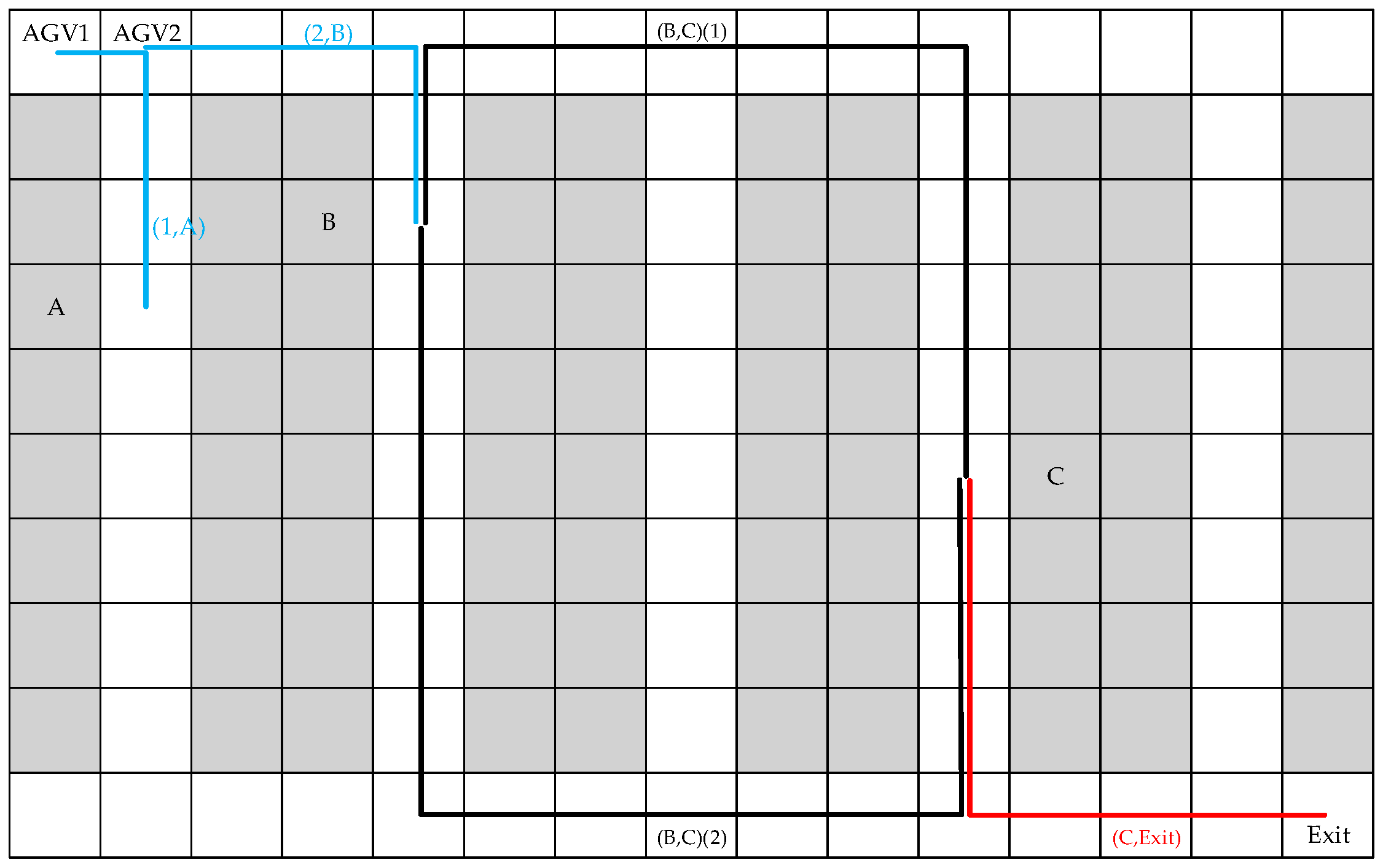
Due to the layout characteristics of the automatic warehouse, the value of ${\mathrm{d}}_{\mathrm{ij}}$ can be calculated as follows, where (${\mathrm{p}}_1$,${\mathrm{p}}_2$) indicates the driving path from point ${\mathrm{p}}_1$ to point ${\mathrm{p}}_2$. Some examples are shown in Figure 2.

(1) The distance from the entrance i to the pickup point j:

$${\mathrm{d}}_{\mathrm{ij}}=\{\begin{array}{c}{(\mathrm{c}}_{\mathrm{j}}-{\mathrm{c}}_{\mathrm{i}}{)+(\mathrm{r}}_{\mathrm{j}}-{\mathrm{r}}_{\mathrm{i}}{),\mathrm{c}}_{\mathrm{i}}{<\mathrm{c}}_{\mathrm{j}}\\ \left({\mathrm{c}}_{\mathrm{i}}-{\mathrm{c}}_{\mathrm{j}}\right)+\left({\mathrm{r}}_{\mathrm{j}}-{\mathrm{r}}_{\mathrm{i}}\right){,\mathrm{c}}_{\mathrm{i}}{>\mathrm{c}}_{\mathrm{j}}\end{array}$$

Path (1, A) and path (2, B) show the cases when ${\mathrm{c}}_{\mathrm{i}}{<\mathrm{c}}_{\mathrm{j}}$.

(2) The distance from the pickup point i to the pickup point j:

If ${\mathrm{c}}_{\mathrm{i}}\ne {\mathrm{c}}_{\mathrm{j}}$:

$${\mathrm{d}}_{\mathrm{ij}}=\{\begin{array}{c}\min \{\left({\mathrm{c}}_{\mathrm{j}}-{\mathrm{c}}_{\mathrm{i}}\right)+\left({\mathrm{r}}_{\mathrm{j}}-{1+\mathrm{r}}_{\mathrm{i}}-1\right),\left({\mathrm{c}}_{\mathrm{j}}-{\mathrm{c}}_{\mathrm{i}}\right)+\left(\mathrm{c}-{\mathrm{r}}_{\mathrm{j}}+\mathrm{c}-{\mathrm{r}}_{\mathrm{i}}\right){\},\mathrm{c}}_{\mathrm{i}}{<\mathrm{c}}_{\mathrm{j}}\\ \min \{\left({\mathrm{c}}_{\mathrm{i}}-{\mathrm{c}}_{\mathrm{j}}\right)+\left({\mathrm{r}}_{\mathrm{j}}-{1+\mathrm{r}}_{\mathrm{i}}-1\right),\left({\mathrm{c}}_{\mathrm{i}}-{\mathrm{c}}_{\mathrm{j}}\right)+\left(\mathrm{c}-{\mathrm{r}}_{\mathrm{j}}+\mathrm{c}-{\mathrm{r}}_{\mathrm{i}}\right){\},\mathrm{c}}_{\mathrm{i}}{>\mathrm{c}}_{\mathrm{j}}\end{array}$$

Otherwise:

$${\mathrm{d}}_{\mathrm{ij}}=\{\begin{array}{c}{\mathrm{r}}_{\mathrm{j}} - {\mathrm{r}}_{\mathrm{i}}{,\mathrm{r}}_{\mathrm{i}}{<\mathrm{r}}_{\mathrm{j}}\\ {\mathrm{r}}_{\mathrm{i}} - {\mathrm{r}}_{\mathrm{j}}{,\mathrm{r}}_{\mathrm{i}}\ge {\mathrm{r}}_{\mathrm{j}}\end{array}$$

Path (B, C) shows the case when ${\mathrm{c}}_{\mathrm{i}}{<\mathrm{c}}_{\mathrm{j}}$. The shortest path between the paths of two driving directions (B, C) (1) and (B, C) (2) is chosen.

(3) The distance from the pickup point i to the entrance j:

$${\mathrm{d}}_{\mathrm{ij}}=\left({\mathrm{r}}_{\mathrm{j}}-{\mathrm{r}}_{\mathrm{i}}\right)+\left({\mathrm{c}}_{\mathrm{j}}-{\mathrm{c}}_{\mathrm{i}}\right)$$

Path (C, Exit) shows this case.

According to the above description, the mathematical programming model of the problem can be obtained as follows:

$$\mathrm{Minimize}\mathrm{Z}={\displaystyle \sum }_{\mathrm{i}=1}^{\mathrm{g}}{\displaystyle \sum }_{\mathrm{j}=1}^{\mathrm{g}}{\displaystyle \sum }_{\mathrm{k}=1}^{\mathrm{m}}{\mathrm{d}}_{\mathrm{ij}}{\mathrm{x}}_{\mathrm{ijk}}+{\displaystyle \sum }_{\mathrm{i}=1}^{\mathrm{g}}{\displaystyle \sum }_{\mathrm{k}=1}^{\mathrm{m}}{\mathrm{d}}_{\mathrm{ki}}{\mathrm{x}}_{\mathrm{kik}} +{\displaystyle \sum }_{\mathrm{i}=1}^{\mathrm{g}}{\displaystyle \sum }_{\mathrm{k}=1}^{\mathrm{m}}{\mathrm{d}}_{\mathrm{ig}}{\mathrm{x}}_{\mathrm{igk}}(\mathrm{i}\ne \mathrm{j},\mathrm{i},\mathrm{j}\in \mathrm{G}\prime )$$

(1)

Subject to:

$${\mathrm{x}}_{\mathrm{ikk}}=0,\forall \mathrm{i}\in {\mathrm{G}}^{\prime },\mathrm{k}=1,2,\dots ,\mathrm{m}$$

(2)

$${\mathrm{x}}_{\mathrm{gik}}=0,\forall \mathrm{i}\in {\mathrm{G}}^{\prime },\mathrm{k}=1,2,\dots ,\mathrm{m}$$

(3)

$${\mathrm{x}}_{\mathrm{gkk}}=0,\forall \mathrm{k}=1,2,\dots ,\mathrm{m}$$

(4)

$${\displaystyle \sum }_{\mathrm{i}=1}^{\mathrm{g}}{\displaystyle \sum }_{\mathrm{k}=1}^{\mathrm{m}}{\mathrm{x}}_{\mathrm{iik}} =0$$

(5)

$${\displaystyle \sum }_{\mathrm{i}=1}^{\mathrm{g}}{\displaystyle \sum }_{\mathrm{j}=1}^{\mathrm{g}}{\displaystyle \sum }_{\mathrm{k}=1}^{\mathrm{m}}{\mathrm{x}}_{\mathrm{ijk}} =1,\mathrm{j}\in \mathrm{G}\prime$$

(6)

$${\displaystyle \sum }_{\mathrm{k}=1}^{\mathrm{m}}{\mathrm{x}}_{\mathrm{kgk}} =0$$

(7)

The objective is represented by Equation (1), which minimizes the total travel distance. Equations (2)–(4), respectively, indicate that in the AGV pickup sequence, the AGV cannot return to the entrance from the pickup point, go to any pickup point from the exit, or go to any entrance from the exit. Equation (5) limits the AGV not to stay at a point after visiting it. Equation (6) restricts the route so that each pickup point is visited only once. Equation (7) states that at least one pickup point should be arranged for each AGV.

3. Conflict Types and Solving Approaches

According to the driving direction of an AGV when a conflict occurs in the path planning process, the conflicts can be divided into two types.

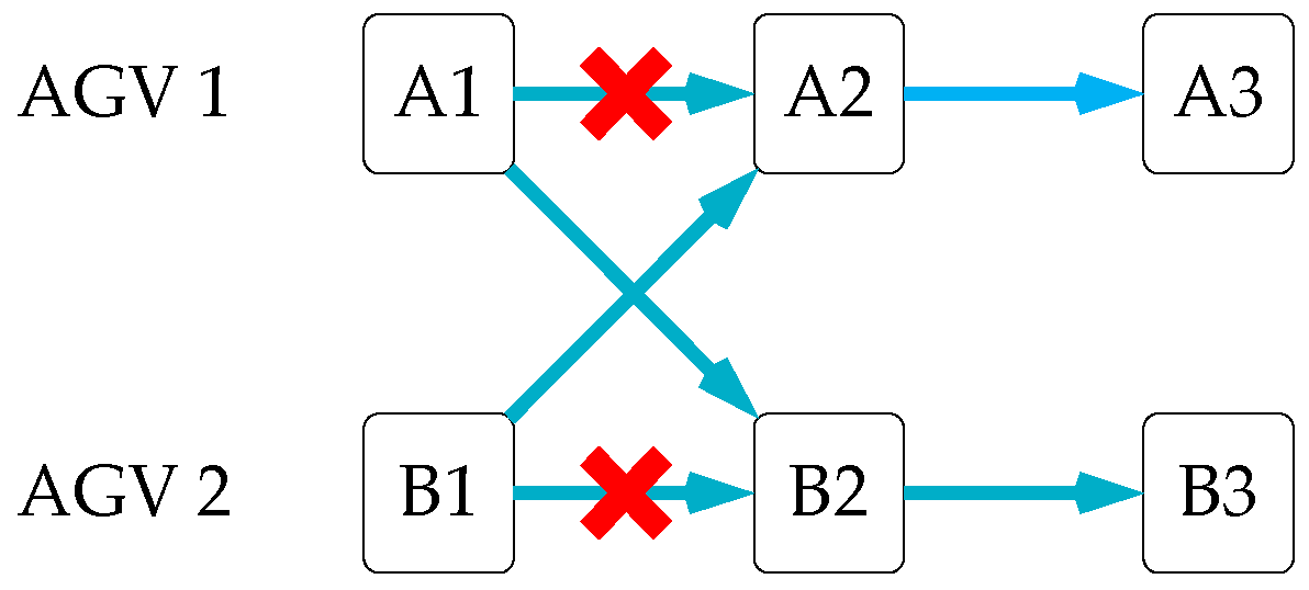
3.1. Opposite Direction Conflict

The opposite direction conflict is the conflict between two AGVs that meet at the same location while running in opposite directions, so they collide with each other. The solution is to swap the subsequent pickup points when two AGVs collide. Figure 3 and Figure 4 show an example. Suppose there is an opposite direction conflict between path A1–A2–A3 and path B1–B2–B3 and the conflict point is at the yellow cell where two AGVs arrive at the same time. Two pickup point sequences and corresponding driving paths before and after eliminating conflicts are shown. The total distance is reduced due to the reduction of overlapping sections.

3.2. Uniform Direction Conflict

The uniform direction conflict is the conflict between two AGVs that meet at the same location while running in same direction, so they collide with each other. The solution is that one AGV waits for time 1, and the AGV that takes shorter time to pass the subsequent path is selected to wait. Figure 5 shows an example: Two AGVs go to right after meeting, and the conflict point is at the yellow cell. Since the subsequent pickup points of each AGV are already arranged when the algorithm runs, the AGV with the shortest time to run the subsequent path can be calculated, and its kept waiting time is 1. For the sake of convenience, we also classified a further conflict that is caused by waiting after solving uniform conflicts as such.

4. Tabu Search Algorithm

4.1. Initial Solution Generation

The method of generating the initial solution is an improvement on the nearest neighbor method:

(1)

First, arrange the first pickup point for each AGV as the one that is closest to the AGV’s entrance.

(2)

Arrange the next nearest pickup point for the AGVs that takes shortest time to pick up all arranged goods.

(3)

Arrange exit after all pickup points have been arranged.

There may be more than one AGV waiting to be arranged in processes (1) and (2), so if some AGVs want to select the same pickup point, the pickup point is assigned to the nearest AGV. In the above process, conflicts need to be checked and dealt with every time a pickup point or exit is arranged.

4.2. Neighborhood Search

We propose a relocation operation and exchanging operation combined with the pickup location of a pickup point. Before every iteration begins, the pickup point sequence of each AGV in the current solution is grouped: Entrances and the exit are grouped separately, and consecutive pickup points that are undertaken at same pickup passageway are divided into a group. Figure 6 shows an example of the grouping results, where the column number of passageway is marked in blue and the warehouse is designed to house 600 cells (20 rows and 30 columns).

4.2.1. Relocation Operation

The relocation operation is to move a group of pickup points from one AGV to another AGV.

The group of pickup points can be spilt by drawing a line between two adjacent points, and then one part can be inserted into another AGV sequence. Figure 7 shows all optional relocation sequences for a group of pickup points.

If another AGV has a group whose passageway number is same, the relocation sequence is combined into the group. Then, the combined sequence is sorted from the smallest to the largest, and the opposite sequence becomes another candidate solution. Figure 8 shows an example of this case: Group 2 in AGV 1 (not be split) is relocated into group 3 in AGV 2.

If another AGV has no group whose passageway number is same, the relocation sequence is relocated into a proper location. Suppose the passageway column number of the relocation sequence is c, and the passageway column numbers of two adjacent groups in another AGV are ${\mathrm{c}}_1$ and ${\mathrm{c}}_2$. The relocation location satisfies the following condition:

$$\mathrm{c}\in [\min \left\{{\mathrm{c}}_1{,\mathrm{c}}_2\right\},\max \left\{{\mathrm{c}}_1{,\mathrm{c}}_2\right\})$$

For example, group 3 in AGV 1 can be relocated to the location between groups 3 and 4 in AGV 2. The split method and the order of relocating are similar.

4.2.2. Exchanging Operation

The exchanging operation is used to exchange a group of pickup points in two AGVs. Suppose that there are three continuous groups at passageway column number ${\mathrm{c}}_1{,\mathrm{c}}_2{,\mathrm{c}}_3$ in AGV 1 and three continuous groups at passageway column number ${\mathrm{c}}_4{,\mathrm{c}}_5{,\mathrm{c}}_6$ in AGV 2. If a group at passageway number ${\mathrm{c}}_2$ in AGV 1 can be exchanged with group at passageway column number ${\mathrm{c}}_5$ in AGV 2 and there are no groups at passageway column number ${\mathrm{c}}_5$ in AGV 1 and no groups at passageway number ${\mathrm{c}}_2$ in AGV 2, the swapped locations should satisfy the following conditions:

$${\mathrm{c}}_2\in [\min \left\{{\mathrm{c}}_4{,\mathrm{c}}_6\right\},\max \left\{{\mathrm{c}}_4{,\mathrm{c}}_6\right\})$$

$${\mathrm{c}}_5\in [\min \left\{{\mathrm{c}}_1{,\mathrm{c}}_3\right\},\max \left\{{\mathrm{c}}_1{,\mathrm{c}}_3\right\})$$

For example, the group at passageway column number 11 in AGV 1 can be exchanged with the group at passageway number 14 in AGV 2. Then two exchanged sequences are sorted and reversed to be candidate solutions, which are similar to those designed in the relocation operation.

4.3. Tabu Object and Aspiration Criterion

The tabu object is the objective function value. If all candidate solutions are tabooed in one of the iterations, the candidate solution with the best objective function value breaks the ban.

4.4. Flow Chart of our TS Algorithm

The tabu object is the objective function value. If all candidate solutions are tabooed in one of the iterations, the candidate solution with the best objective function value breaks the ban.

The concrete procedures of the novel tabu search (NTS) algorithm are expressed as follows.

Step 1: Set parameters, such as tabu list length (TL) and maximum number of iterations (τ_max). The tabu list is set to be empty.

Step 2: Generate the initial solution by using an improved nearest neighbor method. Set the generation as τ = 0.

Step 3: Use improved relocation and exchange operators to generate candidate solution sets. If all candidates are tabooed, go to step 4; otherwise go to step 5.

Step 4: The best solution of candidate solution set breaks the ban and is selected as the current solution. Then, go to step 6.

Step 5: Select the best solution in the candidate solution set that is not tabooed as the current solution. Then, go to step 6.

Step 6: If τ < τmax, set τ = τ + 1, then return to Step 3. Otherwise, go to Step 7.

Step 7: Output the best solution and stop.

The flowchart of the NTS algorithm is shown in Figure 9.

5. Computational Results

In the simulation experiment, the warehouse is divided into 600 cells (20 rows and 30 columns). The relevant control parameters of the algorithm are measured by the orthogonal test design method: a tabu list length of 7 and a maximum number of iterations of 100. The specific process of the orthogonal experimental design of the NTS algorithm is shown in Appendix A. Nine combinations of n = 60, 100, and 140 and m = 3, 5, and 8 were tested. Each combination tested 10 groups of random data and recorded the final objective function value. All algorithms were coded in C++ programming language and implemented on a PC with an Intel Core i5 CPU (1.6 GHz × 4) and 4 GB RAM.

As shown in

Table 2. Computational results of the NTS algorithm, tabu search (TS) algorithm, and differential evolution algorithm with a local search strategy (HDDE) regarding the final objective value.

		n = 60			n = 100			n = 140
		NTS	TS	HDDE	NTS	TS	HDDE	NTS	TS	HDDE
m = 3	Trail 1	281	283	387	277	281	431	285	367	487
	Trail 2	277	277	359	283	295	445	283	369	407
	Trail 3	271	277	385	281	289	367	285	357	481
	Trail 4	279	299	383	283	325	391	281	371	467
	Trail 5	279	293	371	281	285	429	283	297	409
	Trail 6	275	305	369	283	301	487	281	363	483
	Trail 7	275	299	403	281	319	419	285	327	477
	Trail 8	281	285	381	277	293	387	285	313	467
	Trail 9	275	275	377	283	293	483	285	331	477
	Trail 10	273	307	355	283	293	415	285	365	483
	average	277	290	377	281	297	425	284	346	464
m = 5	Trail 1	332	332	488	328	382	576	336	408	600
	Trail 2	328	340	466	334	454	556	334	418	612
	Trail 3	324	334	428	330	370	546	336	360	632
	Trail 4	330	326	488	334	438	582	332	380	612
	Trail 5	330	332	506	332	370	572	334	380	614
	Trail 6	332	344	466	332	340	554	332	388	638
	Trail 7	326	402	508	332	376	628	336	344	632
	Trail 8	328	344	446	330	410	514	336	384	624
	Trail 9	326	348	444	332	362	574	336	370	620
	Trail 10	324	344	462	334	382	552	336	400	648
	average	328	345	470	332	388	565	335	383	623
m = 8	Trail 1	394	432	522	394	482	694	394	510	698
	Trail 2	394	422	540	394	448	676	394	498	742
	Trail 3	392	430	526	406	464	680	394	528	866
	Trail 4	394	394	534	394	460	714	394	478	694
	Trail 5	394	466	530	394	496	676	394	474	712
	Trail 6	394	414	512	394	474	616	394	468	758
	Trail 7	394	420	558	394	488	668	394	510	710
	Trail 8	394	422	514	394	464	716	394	536	786
	Trail 9	394	432	484	394	488	700	394	516	742
	Trail 10	394	402	534	394	460	686	424	470	720
	average	394	423	525	395	472	683	397	499	743

and

Table 3. Computational results of the NTS, TS and HDDE algorithms regarding running time(s).

		n = 60			n = 100			n = 140
		NTS	TS	HDDE	NTS	TS	HDDE	NTS	TS	HDDE
m = 3	Trail 1	1.951	3.079	500.397	3.715	8.128	10393.339	6.934	19.609	18,961.581
	Trail 2	1.976	3.340	481.716	4.195	7.505	6626.229	6.913	19.374	15,427.298
	Trail 3	1.939	3.246	575.057	3.926	8.440	3634.481	7.386	17.116	24,877.259
	Trail 4	1.948	3.393	435.070	3.929	8.798	5256.536	6.945	19.320	19,682.740
	Trail 5	1.945	2.994	727.229	4.019	7.853	3738.185	7.169	14.811	16,561.710
	Trail 6	2.097	3.653	892.122	3.979	8.063	3964.789	6.895	18.527	22,405.243
	Trail 7	1.920	3.544	472.420	3.963	8.769	3698.056	7.130	17.053	16,051.987
	Trail 8	1.836	3.504	506.553	4.180	8.235	4511.152	6.800	15.419	17,810.505
	Trail 9	1.921	3.619	526.601	3.937	8.293	5317.399	6.803	16.498	21,293.276
	Trail 10	1.882	3.255	610.396	3.957	8.216	4840.318	6.902	16.684	19,258.136
	average	1.942	3.363	572.756	3.980	8.230	5198.048	6.988	17.441	19,232.974
m = 5	Trail 1	3.943	5.118	1512.533	8.161	13.505	8391.081	13.857	25.214	23,283.422
	Trail 2	3.744	5.729	1118.698	8.226	15.769	5361.342	14.364	25.011	25,869.500
	Trail 3	4.162	5.285	1415.852	8.122	12.086	6211.561	13.974	22.084	19,439.788
	Trail 4	3.847	5.137	1005.755	8.715	14.787	8971.270	13.817	23.234	19,355.222
	Trail 5	3.943	5.283	1002.492	8.794	12.581	5422.703	14.377	23.769	32,212.212
	Trail 6	4.175	5.018	1660.255	8.335	11.313	5428.650	13.936	23.018	27,777.053
	Trail 7	3.781	6.661	1097.204	9.005	12.915	5506.001	14.149	20.961	18,425.203
	Trail 8	3.926	5.121	747.236	9.171	13.433	7585.026	13.968	22.647	19,667.650
	Trail 9	3.886	5.397	1090.556	8.063	13.870	6643.318	15.191	21.957	26,439.659
	Trail 10	3.831	5.343	774.069	8.194	12.069	7663.535	15.621	24.568	36,381.835
	average	3.924	5.409	1142.465	8.479	13.233	6718.449	14.325	23.246	24,885.154
m = 8	Trail 1	7.909	8.179	3591.557	15.968	21.845	21426.231	26.412	37.348	65,224.116
	Trail 2	7.944	9.163	1993.240	16.141	20.724	16625.712	27.428	37.365	52,793.295
	Trail 3	7.439	8.678	2572.098	16.060	21.320	12983.184	26.943	38.875	40,496.482
	Trail 4	7.476	8.928	2486.247	16.141	20.554	15421.759	26.965	37.227	58,480.069
	Trail 5	7.427	9.956	5021.107	15.853	22.104	21253.317	26.223	35.783	37,094.787
	Trail 6	7.735	9.127	4354.038	16.463	21.325	18642.408	26.408	35.057	59,505.527
	Trail 7	7.310	9.180	1994.660	16.198	20.710	16229.108	26.940	37.375	37,644.008
	Trail 8	7.694	9.268	6158.387	16.981	19.987	12600.642	27.410	40.199	47,251.975
	Trail 9	7.676	9.435	6523.730	15.497	21.908	10957.605	26.486	39.158	36,420.641
	Trail 10	7.538	9.511	5716.876	15.832	20.071	16501.993	26.127	35.850	77,484.502
	average	7.615	9.143	4041.194	16.113	21.055	16264.196	26.734	37.424	51,239.540

, the proposed algorithm (NTS) was compared with two algorithms. Compared with the TS algorithm that used the classical relocation and exchange operators, the NTS algorithm was superior in more than 90% of cases, which proves that the NTS algorithm design is reasonable. Compared with the differential evolution algorithm with a local search strategy (HDDE), from the average running time of each group of experiments, the NTS algorithm ran between 1.942 and 26.734 s, the TS algorithm ran between 3.363 and 37.424 s (and was always slower than the NTS algorithm), while the HDDE algorithm could not get a solution in 60 s. The relative improvement percentage GAP was employed to measure the performance of the NTS algorithm. The GAP can be calculated by Equation (8):

$$\mathrm{GAP}=\frac{{\mathrm{Z}}^{\mathrm{HDDE}}-{\mathrm{Z}}^{\mathrm{NTS}}}{{\mathrm{Z}}^{\mathrm{NTS}}}\times 100\%,$$

(8)

where ${\mathrm{Z}}^{\mathrm{NTS}}$ denotes the average final objective value of the NTS algorithm and ${\mathrm{Z}}^{\mathrm{HDDE}}$ denotes the average final objective value obtained by the HDDE algorithm. Figure 10 shows the trend of the average GAP values.

The following can be observed from Figure 10. With the increase of the number of pickup points n, the average GAP value always became larger and larger. Because of the growing scale of the problem, the differences between the HDDE and NTS algorithms were clearer. With the rise of the number of AGVs m, the average GAP value went up when n = 100 and 140, which was because the number of possible order combinations of pickup points enlarged. When n = 60, the trend did not follow the same pattern, probably due to instability of the NTS algorithm. The high effectiveness of the NTS algorithm is indicated. By improving the neighborhood structure, our NTS algorithm operates on one or more adjacent points and moves them to a reasonable position in a good order to avoid increasing unnecessary path lengths. Thus, our NTS algorithm retains the advantages of the classic TS, with better improvements. However, the classical TS algorithm only operates on one pickup point in the neighborhood operator, which is less flexible than the NTS algorithm. The HDDE algorithm hopes to obtain a better solution by introducing a local search strategy, and the local search operation generates significant time consumption. Due to the randomness of the HDDE algorithm itself, a large number of long paths are generated, and good results cannot be obtained even at the cost of time. Long paths greatly affect the performance of good paths, so a good order cannot be preserved. Therefore, we found that because of the distance between each pair of pickup points in the AGV path problem, the ability to sort the pickup point is key to the performance of the algorithm. The NTS algorithm proposed in this paper solves this problem well and shows the advantage of an intelligent optimization algorithm that is based on neighborhoods, while an intelligent optimization algorithm that is based on population, like the HDDE, is not suitable for solving this problem.

6. Conclusions

Customer requirements are changing, and expectations are rising. Companies are also facing challenges from global competitors that offer customers a wide range of choices via the internet. Intelligent warehouses support enterprises in fierce market competition, overcoming challenges such as demand fluctuation [26]. The normal operation of the warehouse process is the basis of logistics supply chain improvement [27]. With the rapid development of warehouse logistics, the routing optimization of AGVs is playing an important role in improving the efficiency of goods selection and customer satisfaction, thus attracting much attention. An excellent AGV routing scheme can classify and deliver the orders of consumers earlier, which can greatly improve the experience and satisfaction of consumers [28]. The TS algorithm proposed in this article considers situations that may improve the current feasible solutions for designing neighborhood structures, eliminating bad feasible solutions, and accelerating the neighborhood search speeds. Finally, our numerical experiments indicated that this algorithm can improve calculation accuracy when solving the AGV routing problems. Compared with those employed in previous studies, our algorithm adopts conflict resolution methods that do not sacrifice distance, ensure the shortest distance between two points, and try to compress feasible regions to find excellent solutions faster. Therefore, we have found that for AGV path problems, neighborhood-based intelligent optimization algorithms are often more efficient than population-based intelligent optimization algorithms. The improved strategy used by the NTS algorithm that we have proposed s is effective and has strong applicability to AGV path optimization problems in real-life warehouse management.

The main limitation of the proposed algorithm is related to the assumptions that were made in its design process. Some warehouses have a large volume or a high quality of goods, so one AGV may not carry a lot during the actual warehousing process [29]. Once capacity constraints are taken into account, the number of AGVs in and out of storage increases, and the resolution of conflicts becomes more complex.

Due to the variability of such problems and the complexity of solving them, research on such problems is still continuing, and further research will focus on two directions: (1) The solving of multiple objectives optimization problems, such as reducing the maximum pickup time and the number of AGV used, in order to offer a wide range of solutions that represent a balance between objectives and Pareto-based strategies [30]; (2) the consideration of cases when the volume of goods exceeds the AGV ‘s capacity to adapt to the picking processes of different sizes of goods.

References

- Mostafa, N.; Hamdy, W.; Alawady, H. Impacts of Internet of Things on supply chains: A framework for warehousing. Soc. Sci. 2019, 8, 84. [Google Scholar] [CrossRef] [Green Version]
- Richards, G. Warehouse Management: A Complete Guide to Improving Efficiency and Minimizing Costs in the Modern Warehouse, 3rd ed.; Kogan Page: London, UK, 2017; pp. 7–25. [Google Scholar]
- Moshayedi, A.J.; Li, J.; Liao, L. AGV (automated guided vehicle) robot: Mission and obstacles in design and performance. J. Simul. Anal. Nov. Technol. Mech. Eng. 2019, 12, 5–18. [Google Scholar]
- Gotting, H.H. Automation and steering of vehicles in ports. Port Technol. Int. 2000, 10, 101–111. [Google Scholar]
- Liu, J.E.; Zhang, S.; Liu, H. Research on AGV Path Planning under “Parts-to-Picker” Mode. Open J. Soc. Sci. 2019, 7, 1–14. [Google Scholar] [CrossRef] [Green Version]
- Petersen, C.G.; Schmenner, R.W. An evaluation of routing and volume-based storage policies in an order picking operation. Decis. Sci. 1999, 30, 481–501. [Google Scholar] [CrossRef]
- Roodbergen, K.J.; De Koster, R. Routing order pickers in a warehouse with a middle aisle. Eur. J. Oper. Res. 2001, 133, 32–43. [Google Scholar] [CrossRef] [Green Version]
- Grosse, E.H.; Glock, C.H. The effect of worker learning on manual order picking processes. Int. J. Prod. Econ. 2015, 170, 882–890. [Google Scholar] [CrossRef]
- Giannikas, V.; Lu, W.; Robertson, B.; McFarlane, D. An interventionist strategy for warehouse order picking: Evidence from two case studies. Int. J. Prod. Econ. 2017, 189, 63–76. [Google Scholar] [CrossRef] [Green Version]
- Koo, P.H. The use of bucket brigades in zone order picking systems. OR Spectr. 2009, 31, 759. [Google Scholar] [CrossRef]
- Koster, R.D.; Le-Duc, T.; Roodbergen, K.J. Design and control of warehouse order picking: A literature review. Eur. J. Oper. Res. 2007, 182, 481–501. [Google Scholar] [CrossRef]
- Manzini, R. Warehousing in the Global Supply Chain; Springer: London, UK, 2012; pp. 104–137. [Google Scholar]
- Yener, F.; Yazgan, H.R. Optimal warehouse design: Literature review and case study application. Comput. Ind. Eng. 2019, 129, 1–13. [Google Scholar] [CrossRef]
- Dantzig, G.B.; Ramser, J.H. The truck dispatching problem. Manag. Sci. 1959, 6, 80–91. [Google Scholar] [CrossRef]
- Qu, H.; Yi, Z.; Tang, H. A columnar competitive model for solving multi-traveling salesman problem. Chaos Solitons Fractals 2007, 31, 1009–1019. [Google Scholar] [CrossRef]
- Kelly, J.P.; Xu, J. A set-partitioning-based heuristic for the vehicle routing problem. Inf. J. Comput. 1999, 11, 161–172. [Google Scholar] [CrossRef] [Green Version]
- Fan, X.; Luo, X.; Yi, S.; Yang, S.; Zhang, H. Optimal Path Planning for Mobile Robots Based on Intensified Ant Colony Optimization Algorithm. In Proceedings of the 2003 IEEE International Conference on Robotics, Intelligent Systems and Signal, Changsha, China, 8–13 October 2003. [Google Scholar]
- Tian, G.; Zhang, P.; Li, X.; Yin, J.; Lu, F. Research on one class of optimization problem of the automated warehouse using a new kind of hybrid genetic algorithm. J. Syst. Simul. 2004, 16, 1198–1201. [Google Scholar]
- Saska, M.; Macas, M.; Preucil, L.; Lhotska, L. Robot Path Planning Using Particle Swarm Optimization of Ferguson Splines. In Proceedings of the 2006 IEEE Conference on Emerging Technologies and Factory Automation, Prague, Czech Republic, 20–22 September 2006. [Google Scholar]
- Zheng, K.; Tang, D.; Gu, W.; Dai, M. Distributed control of multi-AGV system based on regional control model. Prod. Eng. 2013, 7, 433–441. [Google Scholar] [CrossRef]
- Zhang, B.; Li, L.; Zhao, Y.; Li, J. The Research on E-Commerce Logistics Picking AGV Path Optimization Method Based on the Improved A* Algorithm. In Proceedings of the 2016 International Conference on Cybernetics, Robotics and Control (CRC), Hong Kong, China, 19–21 August 2016. [Google Scholar]
- Kim, D.H.; Hai, N.T.; Joe, W.Y. A Guide to Selecting Path Planning Algorithm for Automated Guided Vehicle (AGV). In Proceedings of the AETA 2017—Recent Advances in Electrical Engineering and Related Sciences: Theory and Application, Ho Chi Minh, Vietnam, 7–9 December 2017. [Google Scholar]
- Zhang, Z.; Guo, Q.; Chen, J.; Yuan, P. Collision-free route planning for multiple agvs in automated warehouse based on collision classification. IEEE Access 2018, 6, 26022–26035. [Google Scholar] [CrossRef]
- Glover, F. Future paths for integer programming and links to artificial intelligence. Comput. Oper. Res. 1986, 13, 533–549. [Google Scholar] [CrossRef]
- Lee, T.K.; Baek, S.H.; Choi, Y.H.; Oh, S.Y. Smooth coverage path planning and control of mobile robots based on high-resolution grid map representation. Robot. Auton. Syst. 2011, 59, 801–812. [Google Scholar] [CrossRef]
- Yerpude, S.; Singhal, T.K. SMART Warehouse with Internet of Things supported Inventory Management System. Int. J. Pure Appl. Math. 2018, 118, 1–15. [Google Scholar]
- Habazin, J.; Glasnović, A.; Bajor, I. Order picking process in warehouse: Case study of dairy industry in Croatia. Promet-Traffic Trans. 2017, 29, 57–65. [Google Scholar] [CrossRef] [Green Version]
- Liu, Y.; Ji, S.; Su, Z.; Guo, D. Multi-objective AGV scheduling in an automatic sorting system of an unmanned (intelligent) warehouse by using two adaptive genetic algorithms and a multi-adaptive genetic algorithm. PLoS ONE 2019, 14, e0226161. [Google Scholar] [CrossRef] [PubMed]
- Zuniga, C.A.; Olivares-Benitez, E.; Tenahua, A.M.; Mujica, M.A. A methodology to solve the Order Batching Problem. IFAC-PapersOnLine 2015, 48, 1380–1386. [Google Scholar] [CrossRef]
- Nosrati, M.; Khamseh, A. Bi objective hybrid vehicle routing problem with alternative paths and reliability. Decis. Sci. Lett. 2020, 9, 145–162. [Google Scholar] [CrossRef]
Figure 1.
Plane diagram of automatic warehouse. (Take three automated guided vehicles (AGVs) as examples, and cells 1–3 are their respective entrances.).
Figure 2.
Examples of calculation method for the travel distance between pickup point (or entrance) i and pickup point (or exit) j ().
Figure 3.
Driving paths before and after eliminating conflicts in opposite direction conflict.
Figure 4.
Pickup points sequences before and after eliminating conflicts in opposite direction conflict.
Figure 5.
Uniform direction conflict when two AGVs meet at the yellow cell and are arranged to go to right.
Figure 6.
Grouping results for two AGVs’ picking sequences in which every group is separated by an arrow.
Figure 7.
Optional relocation sequences including (1)–(7) in group 3 in AGV 1.
Figure 8.
An example in a relocation operator when group 2 in AGV 1 (not be split) is relocated into group 3 in AGV 2.
Figure 9.
Novel tabu search (NTS) algorithm flowchart.
Figure 10.
The average GAP concerning nine combinations of n = 60, 100, and 140 and m = 3, 5, and 8.