A Deep Learning Algorithm for the Max-Cut Problem Based on Pointer Network Structure with Supervised Learning and Reinforcement Learning Strategies

Abstract

The Max-cut problem is a well-known combinatorial optimization problem, which has many real-world applications. However, the problem has been proven to be non-deterministic polynomial-hard (NP-hard), which means that exact solution algorithms are not suitable for large-scale situations, as it is too time-consuming to obtain a solution. Therefore, designing heuristic algorithms is a promising but challenging direction to effectively solve large-scale Max-cut problems. For this reason, we propose a unique method which combines a pointer network and two deep learning strategies (supervised learning and reinforcement learning) in this paper, in order to address this challenge. A pointer network is a sequence-to-sequence deep neural network, which can extract data features in a purely data-driven way to discover the hidden laws behind data. Combining the characteristics of the Max-cut problem, we designed the input and output mechanisms of the pointer network model, and we used supervised learning and reinforcement learning to train the model to evaluate the model performance. Through experiments, we illustrated that our model can be well applied to solve large-scale Max-cut problems. Our experimental results also revealed that the new method will further encourage broader exploration of deep neural network for large-scale combinatorial optimization problems.

1. Introduction

Combinatorial optimization is an important branch of operations research. It refers to solving problems of variable combinations by minimizing (or maximizing) an objective function under given constraints, and is based on the research of mathematical methods to find optimal arrangements, groupings, orderings, or screenings of discrete events. As a research hot-spot in combinatorial optimization, the Max-cut problem is one of the 21 typical non-deterministic polynomial (NP)-complete problems proposed by Richard M. Karp [1]. It refers to obtaining a maximum segmentation for a given directed graph, such that the sum of the weights across all edges of two cutsets is maximized [2]. The Max-cut problem has a wide range of applications in engineering problems, such as Very Large Scale Integration (VLSI) circuit design, statistical physics, image processing, and communications network design [3]. As a solution of the Max-cut problem can be used to measure the robustness of a network [4] and as a standard for network classification [5], it can also be applied to social networks.

It has been discovered that many classic combinatorial optimization problems derived from engineering, economics, and other fields are NP-hard. The Max-cut problem concerned in this paper is among these problems. For combinatorial optimization problems, algorithms can be roughly divided into two categories: one is represented by exact solution approaches, including enumeration methods [6] and branch and bound methods [7], etc. The other category is represented by heuristic algorithms including genetic algorithms, ant colony algorithms, simulated annealing algorithms, neural networks, Lin–Kernighan Heuristic (LKH) algorithms, and so on [8]. However, there is no polynomial time solvable algorithm to find a global optimal solution for NP-hard problems. Compared with the exact approach, heuristic algorithms are able to deal with large-scale problems efficiently. They have certain advantages in computing efficiency and can be applied to solving large-scale problems with huge amount of variables. In order to solve the Max-cut problem, a large number of heuristic algorithms have been proposed, such as evolutionary algorithms and ant colony algorithms. However, for these algorithms, the most obvious disadvantage of them is that they are easy to fall into local optima. For this reason, more and more experts have begun working on the research and innovation of some novel and effective algorithms for large-scale Max-cut problems.

Deep learning is a research field which has developed very rapidly in recent years, achieving great success in many sub-fields of artificial intelligence. From its root, deep learning is a sub-problem of machine learning. Its main purpose is to automatically learn effective feature representations from a large amount of data, such that it can better solve the credit assignment problem (CAP) [9]; that is, the contribution or influence of different components in a system or their parameters to the output of the final system. The emergence of deep neural networks has provided the possibility for solving large-scale combinatorial optimization problems. In recent years, with the development of the combination of deep neural networks and operations research for large-scale combinatorial optimization problems, scholars have explored how to apply deep neural networks in these fields, and have achieved certain results. The related research has mainly focused on the algorithm design for combinatorial optimization problems based on pointer networks. Vinyals used the attention mechanism [10] to integrate a pointer structure into the sequence-to-sequence model, thus creating the pointer network. Bello improved the pointer network structure and used a strategy gradient algorithm combined with time-series difference learning to train the pointer network in reinforcement learning to solve the combinatorial optimization problem [11]. Mirhoseini removed the coding part of a recurrent neural network (RNN) and used the embedded input to replace the hidden state of the RNN. With this modification, the computational complexity was greatly reduced and the efficiency of the model was improved [12]. In Reference [13], a purely data-driven method to obtain approximate solutions of NP-hard problems was proposed. In Reference [14], a pointer network was used to establish a flight decision prediction model. Khalil solved classical combinatorial optimization problems by Q-learning [15]. The pointer network model has also been used, in Reference [16], to solve the weightless Max-cut problem. Similarly, solved the unconstrained boolean quadratic programming problem (UBQP) through the pointer network [17].

The section arrangement of this paper is as follows. Section 2 mainly introduces the Max-cut problem and the method for generating its benchmark. Section 3 demonstrates the pointer network model, including the Long Short-Term Memory network and Encoder–Decoder. Section 4 introduces two ways to train the pointer network model to solve the Max-cut problem, namely supervised learning and reinforcement learning. Section 5 illustrates the details of the experimental procedure and the results. Section 6 provides the conclusions.

2. Motivation and Data Set Structure

2.1. Unified Model of the Max-Cut Problem

The definition of the Max-cut problem is given as follows.

An undirected graph $G=(V,E)$ consists of a set of vertices V and a set of edges E, where $V=\{1,2,\dots ,n\}$ is its set of vertices, and $E\subseteq V\times V$ is its set of edges, and $w_{i,j}$ is the weight on the edge connecting vertex i and vertex j. For any proper subset S of the vertex set V, let:

$$\delta \left(S\right)=\{e_{i,j}\in E;i\in S,j\in V-S\},$$

(1)

where $\delta \left(S\right)$ is a set of edges, one end of which belongs to S and the other end belongs to $V-S$. Then, the cut $cut\left(S\right)$ determined by S is:

$$cut\left(S\right)=\sum _{e_{i,j}\in \delta \left(S\right)}{w}_{i,j}.$$

(2)

In simple terms, the Max-cut problem is to find a segmentation $(S,V-S)$ of a vertex set V, where the maximum weight of the edges is segmented.

2.2. Benchmark Generator of the Max-Cut Problem

When applying deep learning to train and solve the Max-cut problem, whether supervised learning or reinforcement learning, a large number of training samples are necessary. The method of data set generation introduced here is to transform the {−1,1} quadratic programming problem into the Max-cut problem.

First of all, the benchmark generator method for the boolean quadratic programming (BQP) problem, proposed by Michael X. Zhou [18], is used to generate random {−1,1} quadratic programming problems, which can be solved in polynomial time. Next, inspired by [19], we transform the results of the previous step into solutions of the Max-cut problem. The specific implementation is described below.

Michael X. Zhou transformed the quadratic programming problem shown by Equation (3) into the dual problem shown by Equation (4) through the Lagrangian dual method.

$$min\{f\left(x\right)=\frac{1}{2}{x}^{T}Qx-c^{T}x\left|x\in {\{-1,1\}}^n\right.\},$$

(3)

where $Q=Q^T\in {\mathbb{R}}^{n\times n}$ is a given indefinite matrix, and $c\in {\mathbb{R}}^n$ is a given non-zero vector.

The dual problem is described as follows:

$$\begin{array}{c}\mathrm{find}Q,c,x,\lambda \hfill \\ \mathrm{s}.\mathrm{t}.(Q+diag\left(\lambda \right))=c\hfill \\ Q+diag\left(\lambda \right)>0\hfill \\ x\in {\{-1,1\}}^n\hfill \end{array}.$$

(4)

Then, according to the paper [19], the solution of the {−1,1} quadratic programming problem can be transformed into the solution of the Max-cut problem.

The integer programming for the Max-cut problem is given by:

$$\begin{array}{c}max\frac{1}{2}{\displaystyle \sum _{i<j}}{w}_{i,j}(1-x_i·x_j)\hfill \\ \mathrm{s}.\mathrm{t}.x_i\in \{-1,1\},\forall i=1,\dots ,n,\hfill \end{array}$$

(5)

where i in $x_i\in \{-1,1\}$ represents the vertex i, and $-1$ and 1 represent the values of the two sets. If $x_i·x_j$ is equal to 1 and the vertices of edge $(i,j)$ are in the same set, then $(i,j)\in E$ is not a cut edge; if $x_i·x_j$ is equal to $-1$ and the vertices of the edge $(i,j)$ are not in the same set, then $(i,j)\in E$ is the cut edge. If $(i,j)\in E$ is a cut edge, $(1-x_i·x_j)/\phantom{(1-x_i·x_j)2}2$ is equal to 1; if $(i,j)\in E$ is not a cut edge, $(1-x_i·x_j)/\phantom{(1-x_i·x_j)2}2$ is equal to 0. Thus, the objective function represents the sum of the weights of the cut edges of the Max-cut. Define $S=\{i:x_i=1\},\overline{S}=\{i:x_i=-1\}$, and the weight of the cut is $w(S,\overline{S})={\displaystyle \sum _{i<j}}{w}_{i,j}(1-x_i·x_j)/2$.

The pseudocode for generating the benchmark of the Max-cut problem is shown in Algorithm 1, where the parameter $base$ is used to control the value range of the elements in matrix Q.

Algorithm 1 A benchmark generator for the Max-cut problem

Input: Dimension: n; $base=10$;

Output: Matrix: Q; Vector: x

1: Randomly generate an n-dimensional matrix that conforms to the standard normal distribution to obtain Q; 2: $Q=base\times Q$; 3: Convert Q to a symmetric matrix with $\frac{Q+Q^T}{2}$; 4: Generate random numbers in the range (0,1) of n rows and 1 column as a vector x; 5: $x=2x-1$; 6: Take the absolute value of Q and sum it over the rows, assigning the result to $\lambda$; 7: Place the value of the vector $\lambda$ on the main diagonal of the square matrix $Q^{\prime }$ in order, and let the values of $Q^{\prime }$ (except the main diagonal) be zero. 8: $c=(Q+Q^{\prime })\times x$; 9: Set an additional variable $w_{oj}$, $w_{oj}=\frac{1}{4}\left({\displaystyle \sum _{j=1}^{i-1}}{q}_{ji}+{\displaystyle \sum _{j=i+1}^n}{q}_{ij}\right)+\frac{1}{2}{c}_i,1\le j\le n$, and $w_{ij}=\frac{1}{4}{q}_{ij},1\le i<j\le n$; 10: Update Q: $Q=(q_{1j}^T,q_{2j}^T,\dots ,q_{(n+1)j}^T)\leftarrow (w_{0j}^T,w_{1j}^T,\dots ,w_{nj}^T)$; 11: Set an additional variable $x_0=1$, and let $x=2x+1$; 12: Update x: $x=(x_1,x_2,\dots ,x_{n+1})\leftarrow (x_0,x_1,\dots ,x_n)$.

This method for obtaining Max-cut benchmark data sets effectively solves the difficulty in training the network to solve the Max-cut problem model when lacking a large number of training samples. However, there is a common defect in this method: in the training set obtained using the dual problem to deduce the solution of the original problem, its data samples obey certain rules. This may lead to difficulty in learning the general rule of the Max-cut problem when training with the method by deep learning.

Therefore, in addition to the above method, we consider using the benchmark generator in the Biq Mac Library to solve the Max-cut problem. The Biq Mac Library offers a collection of Max-cut instances. Biq Mac is a branch and bound code based on semi-definite programming (SDP). The dimension of the problems (i.e., number of variables or number of vertices in the graph) ranges from 60–100. These instances are mainly used to test the pointer network model for the Max-cut problem.

3. Models

3.1. Long Short-Term Memory

It is difficult for traditional neural networks to classify subsequent events by using previous event information. However, an RNN can continuously operate information in a cyclic manner to ensure that the information persists, thereby effectively processing time-series data of any length. Given an input sequence $x_{1:T}=(x_1,x_2,\dots ,x_t,\dots ,x_T)$, the RNN updates the activity value $h_t$ of the hidden layer with feedback and calculates the output sequence $y_{1:T}=(y_1,y_2,\dots ,y_t,\dots ,y_T)$ using the following equations:

$$h_t=\mathrm{sigmoid}(M^{hx}{x}_t+M^{hh}{h}_{t-1}),$$

(6)

$$y_t=M^{yh}{h}_t.$$

(7)

As long as the alignment between input and output is known in advance, an RNN can easily map sequences to sequences. However, the RNN cannot solve the problem when the input and output sequences have different lengths or have complex and non-monotonic relationships [20]. In addition, when the input sequence is long, the problem of gradient explosion and disappearance will occur [21]; which is also known as the long-range dependence problem. In order to solve these problems, many improvements have been made to RNNs; the most effective way, thus far, is to use a gating mechanism.

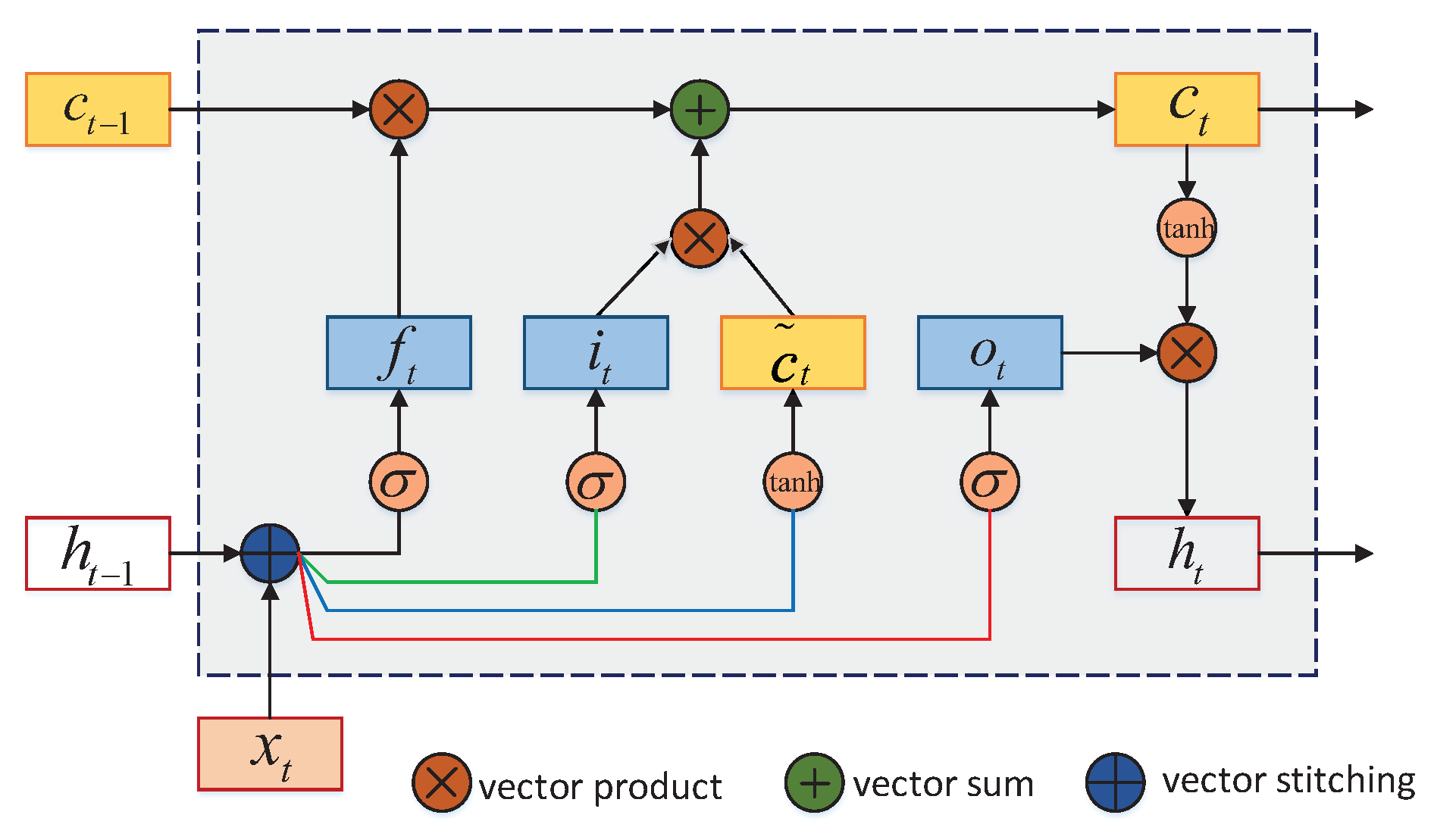
A long short-term memory (LSTM) network [22] is a variant of RNN, which is an outstanding embodiment of RNN based on the gating mechanism. Figure 1 shows the structure of the loop unit of a LSTM. By applying the LSTM loop unit of the gating mechanism, the entire network can establish long-term timing dependencies to better control the path of information transmission. The equations of the LSTM model can be briefly described as:

$$\left[\begin{array}{c}{\tilde{c}}_t\\ o_t\\ i_t\\ f_t\end{array}\right]=\left[\begin{array}{c}\tanh \\ \sigma \\ \sigma \\ \sigma \end{array}\right]\left(M\left[\begin{array}{c}{x}_t\\ h_{t-1}\end{array}\right]+b\right),$$

(8)

$$c_t=f_t\odot c_{t-1}+i_t\odot {\tilde{c}}_t,$$

(9)

$$h_t=o_t\odot \tanh \left(c_t\right),$$

(10)

where $x_t\in {\mathbb{R}}^e$ is the input at the current time; $M\in \mathbb{R}{}^{4d\times (d+e)}$ and $b\in \mathbb{R}{}^{4d}$ are the network parameters; $\sigma (·)$ is the Logistic function, with output interval $(0,1)$; $h_{t-1}$ is the external state at the previous time; ⊙ is the product of vector elements; $c_{t-1}$ is the memory unit at the previous moment; and ${\tilde{c}}_t$ is the candidate state obtained by the non-linear function. At each time t, the internal state $c_t$ of the LSTM records historical information up to the current time. The three gates used to control the path of information transmission are $f_t$, $i_t$, and $o_t$. The functions of three gates are:

• The forget gate $f_t$ controls how much information the previous state $c_{t-1}$ needs to forget;
• The input gate $i_t$ controls how much information the candidate state ${\tilde{c}}_t$ needs to be saved at the current moment; and
• The output gate $o_t$ controls how much information the internal state $c_{t-1}$ of the current moment needs to be output to the external state $h_{t-1}$.

In our algorithm, the purpose of the LSTM is to estimate the conditional probability $p(y_1,\dots ,y_{T^{\prime }}\left|x_1,\dots ,x_T\right.)$, where $(x_1,\dots ,x_T)$ is the input sequence, $y_1,\dots ,y_{T^{\prime }}$ is the corresponding output sequence, and the length $T^{\prime }$ may be different from T. The LSTM first obtains a fixed dimension representation X of the input sequence $(x_1,\dots ,x_T)$ (given by the last hidden state of the LSTM), then calculates $y_1,\dots ,y_{T^{\prime }}$, whose initial hidden state is set to $x_1,\dots ,x_T$:

$$p(y_1,\dots ,y_{T^{\prime }}|x_1,\dots ,x_T)=\prod _{t=1}^{T^{\prime }}p\left(y_t\right|X,y_1,\dots ,y_{t-1}),$$

(11)

where each $p\left(y_t\right|X,y_1,\dots ,y_{t-1})$ distribution is represented by the softmax of all variables in the input Max-cut problem matrix.

3.2. Encoder–Decoder Model

The encoder–decoder model is also called the asynchronous sequence-to-sequence model; that is, the input sequence and the output sequence neither need to have a strict correspondence relationship, nor do they need to maintain the same length. Compared with traditional structures, it greatly expands the application scope of the model. It can directly model sequence problems in a pure data-driven manner and can train the model using an end-to-end method. It can be seen that it is very suitable for solving combinatorial optimization problems.

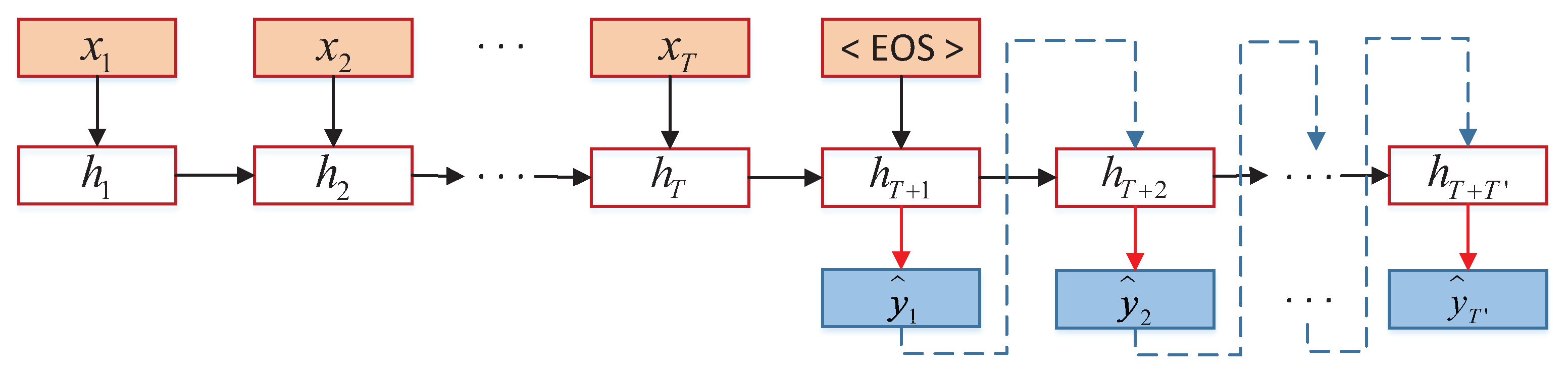
In the encoder–decoder model (shown in Figure 2), the input is a sequence $x_{1:T}=(x_1,\dots ,x_T)$ of length T, and the output is a sequence $y_{1:T^{\prime }}=(y_1,\dots ,y_{T^{\prime }})$ of length $T^{\prime }$. The implementation process is realized by first encoding and then decoding. Firstly, a sample x is input into an RNN (encoder) at different times to obtain its encoding $h_T$. Secondly, another RNN (decoder) is used to obtain the output sequence ${\widehat{y}}_{1:T^{\prime }}$. In order to establish the dependence between the output sequences, a non-linear autoregressive model is usually used in the decoder:

$$h_t=f_1(h_{t-1},x_t),\forall t\in [1,T],$$

(12)

$$h_{T+t}=f_2(h_{T+t-1},{\widehat{y}}_{t-1}),\forall t\in [1,T^{\prime }],$$

(13)

$$y_t=g\left(h_{T+t}\right),\forall t\in [1,T^{\prime }],$$

(14)

where $f_1(·)$ and $f_2(·)$ are RNNs used as encoder and decoder, respectively; $g(·)$ is a classifier; and ${\widehat{y}}_t$ are vector representations used to predict the output.

3.3. Pointer Network

The amount of information that can be stored in a neural network is called the network capacity. Generally speaking, if more information needs to be stored, then more neurons are needed or the network must be more complicated, which will cause the number of necessary parameters of the neural network to increase exponentially. Although general RNNs have strong capabilities, when dealing with complex tasks, such as processing large amounts of input information or complex computing processes, the computing power of computers is still a bottleneck that limits the development of neural networks.

In order to reduce the computational complexity, we use the mechanisms of the human brain to solve the information overload problem. In such a way, we add an attention mechanism to the RNN. When the computing power is limited, it is used as a resource allocation scheme to allocate computing resources to more important tasks.

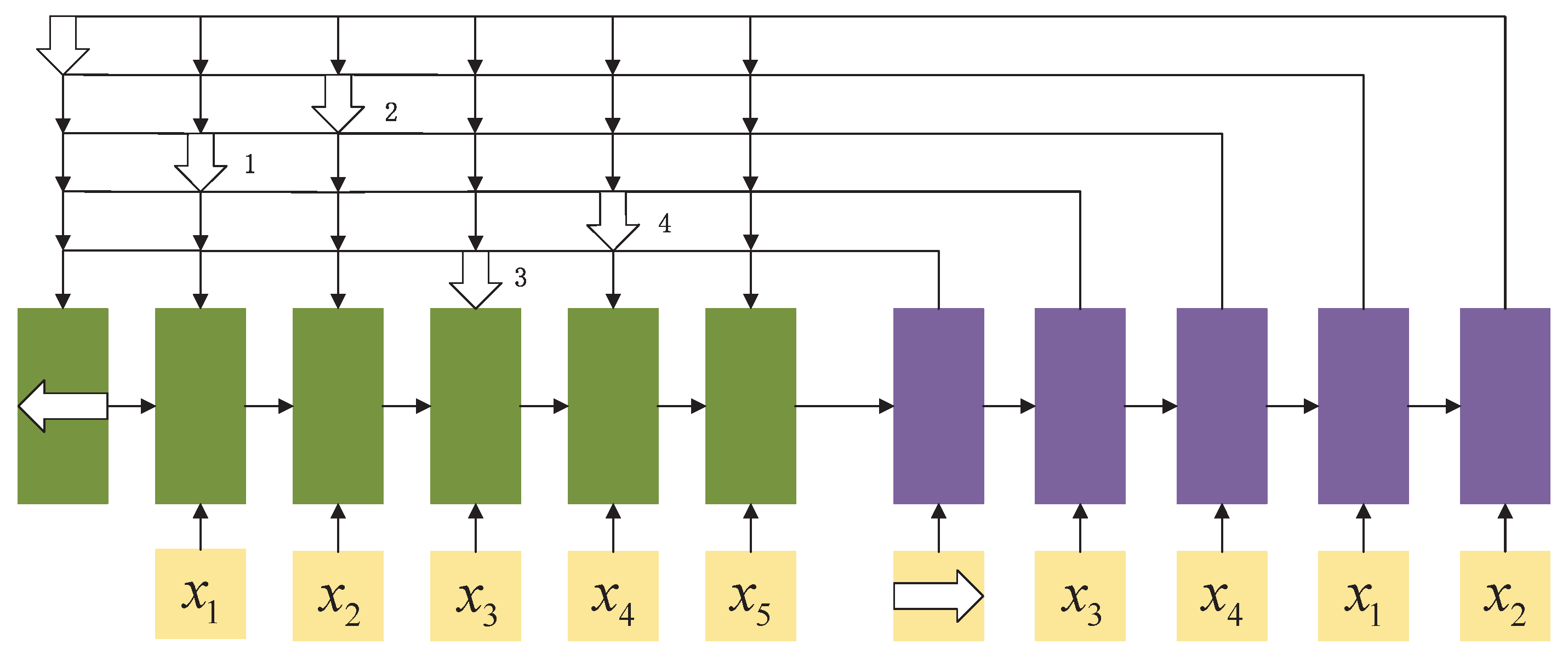
A pointer network is a typical application for combining an attention mechanism and a neural network. We use the attention distribution as a soft pointer to indicate the location of relevant information. In order to save computing resources, it is not necessary to input all the information into the neural network, only the information related to the task needs to be selected from the input sequence X. A pointer network [9] is also an asynchronous sequence-to-sequence model. The input is a sequence $X=x_1,\dots ,x_T$ of length T, and the output is a sequence $y_{1:T^{\prime }}=y_1,y_2,\dots ,y_{T^{\prime }}$. Unlike general sequence-to-sequence tasks, the output sequence here is the index of the input sequence. For example, when the input is a group of out-of-order numbers, the output is the index of the input number sequence sorted by size (e.g., if the input is 20, 5, 10, then the output is 1, 3, 2).

The conditional probability $p\left(y_{1:T^{\prime }}\left|x_{1:T}\right.\right)$ can be written as:

$$\begin{array}{c}p\left(y_{1:T^{\prime }}\left|x_{1:T}\right.\right)={\displaystyle \prod _{i=1}^m}p(y_i\left|y_{1:i-1}\right.,x_{1:T})\hfill \\ \approx {\displaystyle \prod _{i=1}^m}p\left(y_i\left|x_{y_1},\dots ,x_{y_{i-1}},x_{1:T}\right.\right),\hfill \end{array}$$

(15)

where the conditional probability $p\left(y_i\left|x_{y_1},\dots ,x_{y_{i-1}},x_{1:T}\right.\right)$ can be calculated using the attention distribution. Suppose that an RNN is used to encode $x_{y_1},\dots ,x_{y_{i-1}},x_{1:T}$ to obtain the vector $h_i$, then

$$p(y_i\left|y_{1:i-1}\right.,x_{1:T})=\mathrm{softmax}\left(s_{i,j}\right),$$

(16)

where $s_{i,j}$ is the unnormalized attention distribution of each input vector at the ith step of the encoding process,

$$s_{i,j}=v^T\tanh (U_1{x}_j+U_2{h}_i),\forall j\in [1,T],$$

(17)

where v, $U_1$, and $U_2$ are learnable parameters.

Figure 3 shows an example of a pointer network.

4. Learning Mechanism

Machine learning methods can be classified according to different criteria. Generally speaking, according to the information provided by the training samples and different feedback mechanisms, we classify machine learning algorithms into three categories: supervised learning, unsupervised learning, and reinforcement learning. Our algorithm uses supervised learning (SL) and reinforcement learning (RL) to train the pointer network model to obtain the solution of the Max-cut problem, which will be described in detail below.

4.1. Supervised Learning

4.1.1. Input and Output Design

The feature of the Max-cut problem is that its variable is either 0 or 1, such the problem is equivalent to selecting a set of variables from all variables with a value of 1 to maximize the objective function. This is a typical choice problem in combinatorial optimization problems. The goal of supervised learning is to learn the relationship between the input x and the output y by modeling $y=f(x;\theta )$ or $p(y\left|x\right.;\theta )$. For the Max-cut problem, the pointer network uses an $n\times n$ symmetric matrix Q to represent the input sequence of the n nodes, where $q_{ij}$ is an element in the symmetric matrix, which represents the weight of the connection between vertex i vertex and vertex j ($q_{ij}\ge 0$, $q_{ij}=0$ means there is no connection between vertex i and vertex j). The output sequence of the pointer network is represented by $X=x_1,x_2,\dots ,x_n$, which contains two variables; that is 0 and 1. Vertices with 0 and vertices with 1 are divided into two different sets. The result of summing weights with all edges across the two cut sets is the solution to the Max-cut problem.

The following example is used to explain the input and output design of the pointer network to solve the Max-cut problem.

Example 1.

$$\begin{array}{c}f\left(x\right)=3x_1{x}_2+4x_1{x}_4+5x_2{x}_3+2x_2{x}_4+x_3{x}_4\hfill \\ x_i\in \{0,1\},(i=1,\dots ,4)\hfill \end{array}.$$

(18)

The symmetric matrix Q of the above problem can be expressed as:

$$Q=\left(\begin{array}{cccc}0& 3& 0& 4\\ 3& 0& 5& 2\\ 0& 5& 0& 1\\ 4& 2& 1& 0\end{array}\right),$$

and the characteristics of the variables $x_1$, $x_2$, $x_3$, and $x_4$ are represented by the vectors $q_1={(0,3,0,4)}^T$, $q_2={(3,0,5,2)}^T$, $q_3={(0,5,0,1)}^T$, and $q_4={(4,2,1,0)}^T$, respectively.

For the Max-cut problem, the optimal solution of the above example is x. The sequence $(q_1,q_2,q_3,q_4)$ is the input of the pointer network, and the known optimal solution is used to train the network model and guide the model to select $q_1$ and $q_3$. The input vector selected by the decoder represents the corresponding variable value of 1, while the corresponding variable value of the unselected vector is 0.

For the output part of the pointer network model, for the $n\times n$ matrix, we design a matrix of dimension $(n+1)$ to represent the network output. Exactly as in Example 1, the output result is a label that be described by the matrix $O_{label}$:

$$O_{label}=\left(\begin{array}{ccccc}0& 1& 0& 0& 0\\ 0& 0& 0& 1& 0\\ 1& 0& 0& 0& 0\\ 1& 0& 0& 0& 0\\ 1& 0& 0& 0& 0\end{array}\right).$$

The relationship between $O_{label}$ and the variable x is:

$$x_j=\left\{\begin{array}{c}1,\mathrm{if}{o}_{ij}=1,j\ne 0;\hfill \\ \mathrm{EOS},\mathrm{if}{o}_{ij}=1,j=0;\hfill \\ 0,\mathrm{others}.\hfill \end{array}\right.$$

(19)

We use $\mathrm{EOS}={\left(1,0,\cdots ,0\right)}^T$ to indicate the end of the pointer network solution process. After the model training is completed, the probability distribution of the softmax of the output matrix is obtained. The corresponding result may be as described by the matrix $O_{predict}$. In the solution phase, we select the one with the highest probability in the output probability distribution and set it to 1, and the rest of the positions to 0. According to the result of $O_{predict}$, the pointer network selects the variables $x_1$ and $x_3$ with a value of 1, and the remaining variables have a value of 0—which is consistent with the result selected by $O_{label}$:

$$O_{predict}=\left(\begin{array}{ccccc}0.03& 0.8& 0.02& 0.1& 0.05\\ 0.1& 0& 0.2& 0.7& 0\\ 0.9& 0.03& 0.03& 0.01& 0\\ 1& 0& 0& 0& 0\\ 1& 0& 0& 0& 0\end{array}\right).$$

4.1.2. Algorithm Design

When training deep neural networks, for N given training samples ${\left\{\left({\mathbf{x}}^{\left(n\right)},y^{\left(n\right)}\right)\right\}}_{n=1}^N$, the softmax regression in supervised learning uses cross entropy as a loss function and uses gradient descent to optimize the parameter matrix W. The goal of neural network training is to learn the parameters which minimize the value of the cross-entropy loss function. In practical applications, the mini-batch stochastic gradient descent (SGD) method has the advantages of fast convergence and small computational overhead, so, it has gradually become the main optimization algorithm used in large-scale machine learning [23]. Therefore, during the training process, we use mini-batch SGD. At each iteration, we randomly select a small number of training samples to calculate the gradient and update the parameters. Assuming that the number of samples per mini-batch is K, the training process of softmax regression is: initialize $W_0\leftarrow 0$, and then iteratively update by the following equation

$$W_{t+1}\leftarrow W_t+\alpha \left(\frac{1}{K}\sum _{n=1}^N{x}^{\left(n\right)}{(y^{\left(n\right)}-{\widehat{y}}_{W_t}^{\left(n\right)})}^T\right),$$

(20)

where $\alpha$ is the learning rate and ${\widehat{y}}_{W_t}^{\left(n\right)}$ is the output of the softmax regression model when the parameter is $W_t$.

The training process of mini-batch SGD is shown in Algorithm 2.

Algorithm 2 Mini-batch SGD of pointer network

Input: training set: $D={\left\{(x^{\left(n\right)},y^{\left(n\right)})\right\}}_{n=1}^N$; mini-batch size: K; number of training steps: L; learning rate: $\alpha$;

Output: optimal: W

1: random initial W; 2: repeat 3:     randomly reorder the samples in training set D; 4:     for$t=1,\dots ,L$do 5:         select samples $(x^{\left(n\right)},y^{\left(n\right)})$ from the training set D; 6:         update parameters: $W_{t+1}\leftarrow W_t+\alpha \left(\frac{1}{K}{\displaystyle \sum _{n=1}^N}{x}^{\left(n\right)}{(y^{\left(n\right)}-{\widehat{y}}_{W_t}^{\left(n\right)})}^T\right)$; 7:     end for 8: until the error rate of model $f(x;W)$ no longer decreases.

4.2. Reinforcement Learning

Reinforcement learning is a very attractive method in machine learning. It can be described as an agent continuously learning from interaction with the environment to achieve a specific goal (such as obtaining the maximum reward value). The difference between reinforcement learning and supervised learning is that reinforcement learning does not need to give the “correct” strategy as supervised information, it only needs to give the return of the strategy and then adjust the strategy to achieve the maximum expected return. Reinforcement learning is closer to the nature of biological learning and can cope with a variety of complex scenarios, thus coming closer to the goal of general artificial intelligence systems.

The basic elements in reinforcement learning include:

• The $agent$ can sense the state of the external environment and the reward of feedback, then make decisions;
• The $environment$ is everything outside the $agent$, which is affected by the actions of the $agent$ by changing its state and feeding the corresponding reward back to the $agent$;
• s is a description of the $environment$, which can be discrete or continuous, and its state space is S;
• a is a description of the behavior of the $agent$, which can be discrete or continuous, and its action space is A;
• The reward $r(s,a,s^{\prime })$ is a scalar function—that is, after the agent makes an action a based on the current state s, the environment will give a reward to the agent. This reward is related to the state $s^{\prime }$ at the next moment.

For simplicity, we consider the interactions between $agent$ and $environment$ as a discrete time-series in this paper. Figure 4 shows the interaction between an $agent$ and an $environment$.

4.2.1. Input and Output Design

The pointer network input under reinforcement learning is similar to that under supervised learning. The only difference is that, when applying reinforcement learning, a special symbol $Split$ needs to be added, as reinforcement learning only focuses on those variables selected before the variable $Split$. $Split$ is a separator that divides a variable into two types. We use the following rules: when inputting into the pointer network, all variables before $Split$ are set to 1, and all variables after $Split$ are set to 0. We use the zero vector to represent the $Split$. Therefore, in order to change the n-dimensional matrix Q into $n+1$ dimensions, we add a row and a column of 0 to the last row and the last column of matrix Q. Under this rule, taking Example 1 as an example, to convert the matrix Q into the matrix P, the input sequence of the pointer network is $(p_1,p_2,p_3,p_4,Split)$:

$$P=\left(\begin{array}{ccccc}0& 3& 0& 4& 0\\ 3& 0& 5& 2& 0\\ 0& 5& 0& 1& 0\\ 4& 2& 1& 0& 0\\ 0& 0& 0& 0& 0\end{array}\right).$$

Similar to supervised learning, at the output of the pointer network, a symbol $\mathrm{EOS}$ is added to divide the set of output vertices. As in Example 1, the output of the pointer network is $\left(1,3,\mathrm{EOS},2,4\right)$, which means that the four vertices are divided into two sets, which are $\left(1,3\right)$ and $\left(2,4\right)$. The numbers in front of $\mathrm{EOS}$ indicate that the value at these vertex positions is 1, and the numbers after $\mathrm{EOS}$ indicate that the value at these positions is 0. Thus, the max-cut value can be calculated according to the divided sets, and it is this value that is used as the reward in reinforcement learning.

4.2.2. Actor–Critic Algorithm

The actor–critic algorithm is a reinforcement learning method which combines a policy gradient and temporal difference learning. We combine the input–output structure characteristics of the Max-cut problem with the actor–critic algorithm in reinforcement learning to train the pointer network model. The actor–critic algorithm used for solving such combinatorial optimization problems uses the same pointer network encoder for both the actor network and the critic network. First, the actor network encodes the input sequence. Next, the decoder part selects the variable with value 1, according to the probability. The critic network encodes the input sequence, then predicts the optimal value of the Max-cut problem using a value function.

In the actor–critic algorithm, $\varphi \left(s\right)$ is the input to the actor network, which corresponds to the given symmetric matrix Q in the Max-cut problem; that is, Q is used as the input sequence of the actor network. The actor refers to the policy function ${\pi }_{\theta }(s,a)$, which can learn a strategy to obtain the highest possible reward. For the Max-cut problem, ${\pi }_{\theta }(s,a)$ represents the strategy scheme in which variables are selected as 1. The critic refers to the value function $V_{\varphi }\left(s\right)$, which estimates the value function of the current strategy. With the help of the value function, the actor–critic algorithm can update the parameters in a single step, without having to wait until the end of the round to update. In the actor–critic algorithm, the policy function ${\pi }_{\theta }(s,a)$ and the value function $V_{\varphi }\left(s\right)$ are both functions that need to be learned simultaneously during the training process.

Assuming the return $G\left({\tau }_{t:T}\right)$ from time t, we use Equation (21) to approximate it:

$$\widehat{G}\left({\tau }_{t:T}\right)=r_{t+1}+\gamma V_{\varphi }\left(s_{t+1}\right),$$

(21)

where $s_{t+1}$ is the state at $t+1$ and $r_{t+1}$ is the instant reward.

In each step of the update, the strategy function ${\pi }_{\theta }(s,a)$ and the value function $V_{\varphi }\left(s\right)$ are learned. On one hand, the parameter $\varphi$ is updated, such that the value function $V_{\varphi }\left(s_t\right)$ is close to the estimated real return $\widehat{G}\left({\tau }_{t:T}\right)$:

$$\underset{\varphi }{min}{\left(\widehat{G}\left({\tau }_{t:T}\right)-V_{\varphi }\left(s_t\right)\right)}^2.$$

(22)

On the other hand, the value function $V_{\varphi }\left(s_t\right)$ is used as a basis function to update the parameter, in order to reduce the variance of the policy gradient:

$$\theta \leftarrow \theta +\alpha {\gamma }^t\left(\widehat{G}\left({\tau }_{t:T}\right)-V_{\varphi }\left(s_t\right)\right)\frac{\partial }{\partial \theta }log{\pi }_{\theta }\left(a_t|s_t\right).$$

(23)

In each update step, the actor performs an action a, according to the current environment state s and the strategy ${\pi }_{\theta }\left(a\left|s\right.\right)$; the environment state becomes $s^{\prime }$ and the actor obtains an instant reward r. The critic (value function $V_{\varphi }\left(s\right)$) adjusts its own scoring standard, according to the real reward given by the environment and the previous score $(r+\gamma V_{\varphi }\left(s^{\prime }\right))$, such that its own score is closer to the real return of the environment. The actor adjusts its strategy ${\pi }_{\theta }$ according to the critic’s score, and strives to do better next time. At the beginning of the training, actors performs randomly and critic gives random marks. Through continuous learning, the critic’s ratings become more and more accurate, and the actor’s movements become better and better.

Algorithm 3 shows the training process of the actor–critic algorithm.

Algorithm 3 Actor–critic algorithm

Input: state space: S; action space: A; differentiable strategy function: ${\pi }_{\theta }\left(a\left|s\right.\right)$; differentiable state value function: $V_{\varphi }\left(s\right)$; discount rate: $\gamma$; learning rate: $\alpha >0,\beta >0$;

Output: strategy: ${\pi }_{\theta }$

1: random initial $\theta$, $\varphi$; 2: repeat 3:     initial starting state s; 4:     $\lambda =1$; 5:     repeat 6:         In state s, select an action $a={\pi }_{\theta }\left(a\left|s\right.\right)$; 7:         perform the action a to get an instant reward r and a new state $s^{\prime }$; 8:         $\delta \leftarrow r+\gamma V_{\varphi }\left(s^{\prime }\right)-V_{\varphi }\left(s\right)$; 9:         $\varphi \leftarrow \varphi +\beta \delta \frac{\partial }{\partial \varphi }{V}_{\varphi }\left(s\right)$; 10:         $\theta \leftarrow \theta +\alpha \lambda \delta \frac{\partial }{\partial \theta }log{\pi }_{\theta }\left(a\right|s)$; 11:         $\lambda \leftarrow \gamma \lambda$; 12:         $s\leftarrow s^{\prime }$; 13:     until s is the termination state; 14: untilθ converges.

5. Experimental Results and Analysis

Based on the TensorFlow framework, this paper uses two learning strategies (supervised learning and reinforcement learning) to train and predict the Max-cut problem with a pointer network. The model is trained on a deep learning server platform consisting of two NVIDIA TITAN Xp GPUs and an Intel Core i9-7960X CPU.

The initial parameters in the pointer network are randomly generated by a uniform distribution in [−0.08, 0.08], and the initial learning rate is 0.001. During the training process, when supervised learning is applied to train the pointer network, the model uses a single-layer LSTM with 256 hidden units and is trained with mini-batch SGD. When applying reinforcement learning to train the pointer network, the model uses three layers of LSTMs, with each layer consisting of 128 hidden units, and is trained with the actor–critic algorithm. In the prediction stage, the heat parameter in the pointer network is set to 3, and the initial reward baseline is set to 100. The model tested during the prediction phase is the last iteration of the training phase. For the Max-cut problem of different dimensions, except for increasing the sequence length, the other hyperparameter settings are the same. In the implementation, we use the Adam algorithm to adjust the learning rate. Adam algorithm can make effective dynamic adjustments to the model to make the changes in hyperparameters relatively stable [24].

We constructed a data set based on the method mentioned in Section 2.2 (using the {−1,1} quadratic programming problem transformed into the Max-cut problem), which we refer to as the Zhou data set. In order not to lose generality, we also used the Binary quadratic and Max cut Libraries (Biq Mac Library), which are the most commonly used benchmark generators for the Max-cut problem. We performed experiments on the Zhou data set and the Biq Mac Library data set, respectively.

5.1. Experiments on Zhou Data Set

According to the method for randomly generating Max-cut problems in Section 2.2, a large number of Max-cut problems with known exact solutions were obtained, which we formed into data sets with specified input and output formats. The training set and the test set are both data generated from the same probability distribution, and the density of the input matrix Q in the data sample is 94.6%. Each sample in the training and test sets is unique. Then, we divided the data sets randomly into training and test sets according to the ratio of 10:1. For different dimensions, the training set contained 1000 samples and the test set contained 100 samples. The maximum number of training iterations was set to 100,000. The accuracy of the solution trained by the model is defined as:

$$\mathrm{Accuracy}=\frac{v\left(\mathrm{Ptr}-\mathrm{Net}\right)}{v\left(\mathrm{Opt}\right)}\times 100\%,$$

(24)

where $v\left(\mathrm{Ptr}-\mathrm{Net}\right)$ is the solution of trained pointer network model, and $v\left(\mathrm{Opt}\right)$ is the optimal value of the Max-cut problem.

We first used supervised learning to train the pointer network on the 10-, 30-, 50-, 60-, 70-, 80-, 90-, 100-, 150-, and 200-dimensional Max-cut problems, respectively.

Table 1. Average accuracies and training times for Max-cut problems with different dimensions by SL.

Dimensions	Average Accuracy	Average Training Time
10	100%	1:13:20
30	98.78%	2:12:35
50	97.56%	5:29:16
60	94.51%	6:37:10
70	90.95%	7:33:42
80	88.64%	8:39:08
90	86.35%	9:58:06
100	80.50%	11:14:57
150	74.94%	14:52:46
200	71.95%	19:28:25

shows average accuracy of the Max-cut problem of the above dimensions. And the detailed experimental results are listed in

Table 2. Detailed solutions and accuracies for Max-cut problems with different dimensions by supervised learning (SL).

Sample	Optimum	Solution	Accuracy				Sample	Optimum	Solution	Accuracy
S10.1	330	330	100%				S80.1	85,462	74,634	87.33%
S10.2	281	281	100%				S80.2	94,552	83,357	88.16%
S10.3	240	240	100%				S80.3	100,512	82,782	82.36%
S10.4	236	236	100%				S80.4	92,108	83,735	90.91%
S10.5	171	171	100%				S80.5	89,311	79,299	88.79%
S10.6	124	124	100%				S80.6	100,862	97,624	97.79%
S10.7	208	208	100%				S80.7	88,919	81,996	92.21%
S10.8	230	230	100%				S80.8	91,045	79,974	87.84%
S10.9	245	245	100%				S80.9	87,873	75,870	86.34%
S10.10	257	257	100%				S80.10	111,327	95,374	85.67%
S30.1	4861	4861	100%				S90.1	136,959	114,251	83.42%
S30.2	5820	5698	97.90%				S90.2	134,022	124,033	92.55%
S30.3	4708	4617	98.07%				S90.3	145,727	115,448	79.22%
S30.4	6123	6123	100%				S90.4	132,287	117,391	88.74%
S30.5	6033	6008	99.59%				S90.5	134,420	126,341	93.99%
S30.6	5380	5342	99.29%				S90.6	133,817	116,491	87.05%
S30.7	6927	6799	98.15%				S90.7	142,957	123,292	86.24%
S30.8	4914	4741	96.48%				S90.8	120,026	104,207	86.82%
S30.9	6401	6340	99.05%				S90.9	145,635	120,749	82.91%
S30.10	5185	5147	99.27%				S90.10	141,741	117,019	82.56%
S50.1	24,468	23,386	95.58%				S100.1	174,947	144,963	82.86%
S50.2	22,462	21,646	96.37%				S100.2	199,441	181,966	91.24%
S50.3	23,246	23,246	100%				S100.3	166,682	130,995	78.59%
S50.4	19,776	19,273	97.46%				S100.4	179,885	146,426	81.40%
S50.5	25,057	23,947	95.57%				S100.5	184,363	146,653	79.55%
S50.6	27,510	27,037	98.28%				S100.6	191,636	165,283	86.25%
S50.7	26,698	26,368	98.76%				S100.7	189,959	136,784	72.01%
S50.8	20,627	20,261	98.23%				S100.8	177,545	144,373	81.32%
S50.9	20,493	20,213	98.63%				S100.9	181,022	145,642	80.46%
S50.10	22,130	21,404	96.72%				S100.10	189,239	134,965	71.32%
S60.1	43,173	40,062	92.79%				S150.1	542,081	453,348	83.63%
S60.2	42,057	39,280	93.40%				S150.2	571,793	390,333	68.26%
S60.3	43,190	40,360	93.45%				S150.3	678,393	551,327	81.27%
S60.4	54,174	53,138	98.09%				S150.4	574,523	481,574	83.82%
S60.5	43,638	40,180	92.08%				S150.5	545,008	412,718	75.73%
S60.6	38,255	37,333	97.59%				S150.6	613,130	467,820	76.30%
S60.7	52,689	49,260	93.49%				S150.7	545,500	354,314	64.95%
S60.8	43,902	40,741	92.80%				S150.8	632,578	521,155	82.39%
S60.9	39,098	37,980	97.14%				S150.9	612,560	349,406	57.04%
S60.10	41,005	38,655	94.27%				S150.10	630,733	479,420	76.01%
S70.1	64,914	59,371	91.46%				S200.1	1,444,264	1,080,545	74.82%
S70.2	63,306	62,872	99.31%				S200.2	1,488,701	1,006,851	67.63%
S70.3	71,127	62,855	88.37%				S200.3	1,368,359	1,052,517	76.92%
S70.4	65,673	57,286	87.23%				S200.4	1,352,301	1,102,923	81.56%
S70.5	59,045	54,864	92.92%				S200.5	1,309,815	1,152,570	87.99%
S70.6	60,016	50,337	83.87%				S200.6	1,338,423	928,162	69.35%
S70.7	63,158	57,117	90.44%				S200.7	1,311,058	805,257	61.42%
S70.8	63,478	59,211	93.28%				S200.8	1,462,304	822,691	56.26%
S70.9	67,019	60,871	90.83%				S200.9	1,350,077	1,114,423	82.55%
S70.10	70,616	64,818	91.79%				S200.10	1,347,381	822,037	61.01%

.

Then the pointer network based on reinforcement learning was also trained with the Zhou data set, on 10-, 50-, 150-, 200-, 250-, and 300-dimensional Max-cut problems.

Table 3. Average accuracies and training times for Max-cut problems with different dimensions by RL.

Dimensions	Average Accuracy	Average Training Time
10	100%	0:10:07
50	98.28%	0:23:03
100	96.32%	0:42:33
150	95.06%	1:03:57
200	92.38%	1:27:18
250	89.88%	1:53:28
300	87.64%	2:21:30

shows the average accuracy of the Max-cut problem for the above dimensions. And the detailed experimental results are listed in

Table 4. Detailed solutions and accuracies for Max-cut problems with different dimensions by reinforcement learning (RL).

Sample	Optimum	Solution	Accuracy				Sample	Optimum	Solution	Accuracy
R10.1	233	233	100%				R150.6	584,968	572,689	97.90%
R10.2	248	248	100%				R150.7	553,878	453,361	81.86%
R10.3	193	193	100%				R150.8	618,615	583,545	94.33%
R10.4	192	192	100%				R150.9	529,739	522,427	98.62%
R10.5	302	302	100%				R150.10	559,414	513,463	91.79%
R10.6	187	187	100%				R200.1	1,274,866	1,267,884	99.45%
R10.7	341	341	100%				R200.2	1,392,200	1,165,174	83.69%
R10.8	133	133	100%				R200.3	1,358,320	1,345,870	99.07%
R10.9	301	301	100%				R200.4	1,320,006	1,118,705	84.75%
R10.10	272	272	100%				R200.5	1,368,199	1,020,056	74.55%
R50.1	25,565	25,302	98.97%				R200.6	1,397,432	1,292,628	92.50%
R50.2	22,528	22,441	99.61%				R200.7	1,421,061	1,420,172	99.94%
R50.3	25,426	24,783	97.47%				R200.8	1,376,229	1,357,875	98.67%
R50.4	25,787	25,425	98.60%				R200.9	1,344,436	1,266,442	94.20%
R50.5	21,030	19,755	93.94%				R200.10	1,388,152	1,332,225	95.97%
R50.6	25,079	24,614	98.15%				R250.1	2,590,918	2,242,263	86.54%
R50.7	22,077	21,820	98.84%				R250.2	2,700,294	2,503,768	92.72%
R50.8	28,899	28,715	99.36%				R250.3	2,542,443	2,230,460	87.73%
R50.9	29,101	28,614	98.33%				R250.4	2,542,413	2,357,060	92.71%
R50.10	25,729	25,607	99.53%				R250.5	2,702,833	2,547,463	94.25%
R100.1	187,805	182,369	97.02%				R250.6	2,764,901	2,750,197	99.47%
R100.2	197,470	193,171	97.82%				R250.7	2,777,948	2,027,296	72.98%
R100.3	187,495	185,929	99.16%				R250.8	2,671,835	2,530,103	94.70%
R100.4	216,339	211,431	97.73%				R250.9	2,593,131	2,031,284	78.33%
R100.5	161,961	161,067	99.45%				R250.10	2,596,843	2,579,798	99.34%
R100.6	178,737	176,723	98.87%				R300.1	4,430,263	3,858,903	87.10%
R100.7	183,560	183,315	99.87%				R300.2	4,363,482	2,344,354	53.73%
R100.8	155,038	154,292	99.52%				R300.3	4,459,682	4,248,761	95.27%
R100.9	191,120	142,059	74.33%				R300.4	4,562,319	2,369,015	51.93%
R100.10	174,202	173,729	99.73%				R300.5	4,404,895	4,113,113	93.38%
R150.1	568,452	554,128	97.48%				R300.6	4,497,912	4,483,644	99.68%
R150.2	549,303	542,731	98.80%				R300.7	4,364,640	4,298,760	98.49%
R150.3	672,601	628,655	93.47%				R300.8	4,589,744	4,372,106	95.26%
R150.4	590,417	553,860	93.81%				R300.9	4,655,631	4,652,613	99.94%
R150.5	563,674	561,554	99.62%				R300.10	4,956,332	4,944,887	99.77%

.

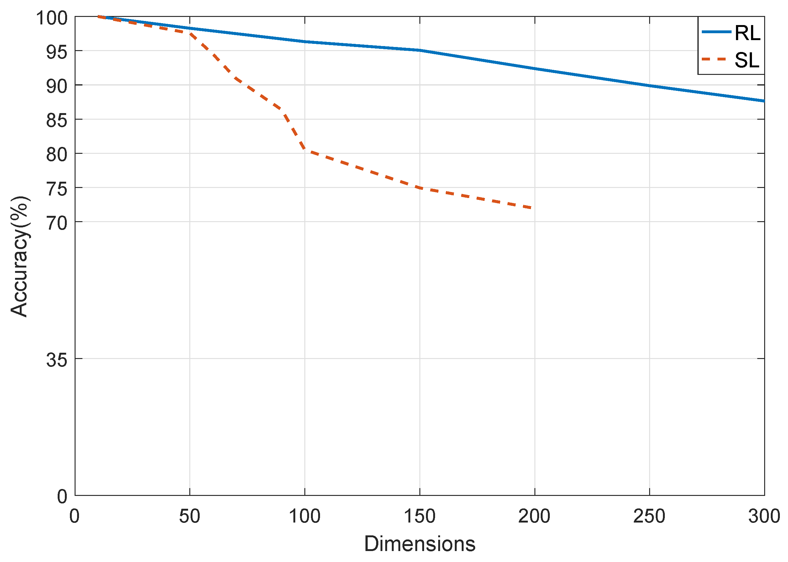
It can be seen, from Table 1 and Table 3 that, regardless of whether supervised learning or reinforcement learning was used, the average accuracy of the pointer network solution decreased as the number of dimensions increased. However, the average accuracy of reinforcement learning decreased very slightly. Secondly, by comparing the two tables, we find that the pointer network model obtained through reinforcement learning was more accurate than that obtained by supervised learning. Finally, it can be seen that the time taken to train the model with reinforcement learning was faster than that for supervised learning. Figure 5 shows the accuracy of the solution for the Max-cut problem samples trained with supervised learning and reinforcement learning.

5.2. Experiments on Biq Mac Library

In order to further verify the generalization ability of the pointer network model, ten groups of 60-, 80-, and 100-dimensional Max-cut samples were selected from the Biq Mac Library (http://biqmac.uni-klu.ac.at/biqmaclib.html). As the Max-cut problem data set of each dimension in the Biq Mac Library only has ten groups of data, the amount of data was not enough to train the pointer network (training the pointer network model requires at least 100 groups of data), so we only used the Biq Mac Library as the test set; the Zhou data set was still used as the training set.

Table 5. Solution and accuracy on Biq Mac Library data set by RL.

Sample	Optimum	Solution	Accuracy				Sample	Optimum	Solution	Accuracy
R60.1	536	441	82.28%				R80.6	926	817	88.23%
R60.2	532	478	89.85%				R80.7	929	773	83.21%
R60.3	529	463	87.52%				R80.8	929	785	84.50%
R60.4	538	478	88.85%				R80.9	925	830	89.73%
R60.5	527	486	92.22%				R80.10	923	640	69.34%
R60.6	533	479	89.87%				R100.1	2019	1530	75.78%
R60.7	531	438	82.49%				R100.2	2060	1507	73.16%
R60.8	535	473	88.41%				R100.3	2032	1461	71.90%
R60.9	530	468	88.30%				R100.4	2067	1573	76.10%
R60.10	533	483	90.62%				R100.5	2039	1433	70.28%
R80.1	929	829	89.24%				R100.6	2108	1483	70.35%
R80.2	941	753	80.02%				R100.7	2032	1464	72.04%
R80.3	934	824	88.22%				R100.8	2074	1585	76.42%
R80.4	923	819	88.73%				R100.9	2022	1477	73.05%
R80.5	932	805	86.37%				R100.10	2005	1446	72.20%

shows the detailed experimental results of the Max-cut problem with 60, 80, and 100 dimensions using the Biq Mac Library by reinforcement learning.

The average prediction results are shown in

Table 6. Average accuracies of different dimensional Max-cut problems using the Biq Mac Library by RL.

Dimensions	Average Accuracy
60	88.05%
80	84.76%
100	73.09%

.

It can be seen, from Table 3 and Table 6, that the average accuracies when predicting the Biq Mac Library using reinforcement learning were lower than the accuracies on Zhou dataset. This is because the Biq Mac Library is composed of data samples with different distributions, which can better characterize the essential characteristics of the Max-cut problem. We believe that, in future research, if the model can be trained on a larger training set with the distribution of the Biq Mac Library, its performance can be definitely improved.

6. Conclusions

In this paper, we proposed an effective deep learning method based on a pointer network for the Max-cut problem. We first analyzed the structural characteristics of the Max-cut problem and introduced a method to generate a large data set of Max-cut problems. Then, the algorithmic frameworks for training the pointer network model under two learning strategies (supervised learning and reinforcement learning) were introduced in detail. We applied supervised learning and reinforcement learning strategies separately to train the pointer network model, and experimented with Max-cut problems with different dimensions. The experimental results revealed that, for the low-dimensional Max-cut problem (below 50 dimensions), the models trained by supervised learning and reinforcement learning both have high accuracy and that the accuracies are basically consistent. For high-dimensional cases (above 50 dimensions), the accuracy of the solution in the training mode using reinforcement learning was significantly better than that with supervised learning. This illustrates that reinforcement learning can better discover the essential characteristics behind the Max-cut problem and can mine better optimal solutions from the data. This important finding will instruct us to further improve the performance and potential of pointer networks as a deep learning method for Max-cut problems and other combinatorial optimization problems in future research.