Diagnostic Analytics for an Autoregressive Model under the Skew-Normal Distribution


1
School of Statistics and Information, Shanghai University of International Business and Economics, Shanghai 201620, China
2
School of Mathematics, Shanghai University of Finance and Economics, Shanghai 200433, China
3
School of Industrial Engineering, Pontificia Universidad Católica de Valparaíso, Valparaíso 2362807, Chile
4
Faculty of Science and Technology, University of Canberra, Bruce, ACT 2617, Australia
5
School of Engineering in Statistics, Universidad Católica del Maule, Talca 3466706, Chile
*
Author to whom correspondence should be addressed.
Mathematics 2020, 8(5), 693; https://0-doi-org.brum.beds.ac.uk/10.3390/math8050693
Submission received: 19 March 2020
/
Revised: 20 April 2020
/
Accepted: 22 April 2020
/
Published: 2 May 2020
(This article belongs to the Special Issue Statistical Simulation and Computation)
Abstract
:Autoregressive models have played an important role in time series. In this paper, an autoregressive model based on the skew-normal distribution is considered. The estimation of its parameters is carried out by using the expectation–maximization algorithm, whereas the diagnostic analytics are conducted by means of the local influence method. Normal curvatures for the model under four perturbation schemes are established. Simulation studies are conducted to evaluate the performance of the proposed procedure. In addition, an empirical example involving weekly financial return data are analyzed using the procedure with the proposed diagnostic analytics, which has improved the model fit.
1. Introduction
For time series data analysis, autoregressive (AR) modeling is an essential technique and has been applied in many areas including biology, chemistry, earth sciences, economics, education, engineering, finance, health, medicine, and physics; see, for example, [1,2] for recent accounts of time series modeling and applications. Issues related to estimation and testing for AR models are extensive and well-established; see [3,4] for related issues to statistical diagnostics which are of equal importance. Local influence diagnostics is the study of how relevant minor perturbations impact the fit of the model and the results of statistical inference. This has become a useful statistical methodology after [5] introduced the idea of local influence to aid in the identification of potentially influential observations. Diagnostic analytics is used in a number of regression and time series models. Among others, Refs. [6,7,8,9,10,11,12,13,14,15] investigated the local influence of linear or nonlinear regression models under non-normal distributional assumptions. In a framework of time series data, Refs. [16,17,18] considered influence diagnostics for AR and vector AR models under normal or elliptical distributions.
A standard assumption for time series models is that their errors are mutually independent and follow normal or symmetric distributions, as studied in [16,17,18]. However, it is known that certain financial and other datasets feature errors with skewed distributions. In order to deal with such data, the skew-normal (SN) distribution and its scale-mixtures have provided an appealing alternative and can therefore be adopted. Their properties, extensions, and applications are becoming increasingly popular; see [19,20,21,22,23,24,25,26]. In addition, Refs. [27,28,29] studied SN linear, linear mixed, and nonlinear models. Ref. [8] analyzed diagnostics in the nonlinear model with scale mixtures of SN and AR errors. For particular financial applications, Ref. [30] looked at asset pricing issues with return data following SN models. To our knowledge, no study on influence diagnostics in AR time series models under SN distributions have been reported. Therefore, the objective of the present paper is to formulate an AR model under the SN distribution (SN AR model) and to derive diagnostic analytics with applications to financial data. We use the matrix differential calculus pioneered by [31] to establish the mathematical results used in our data analysis. We implement the maximum likelihood (ML) method with the expectation–maximization (EM) algorithm to estimate the SN AR model parameters, whereas the local influence method with four perturbation schemes is used for the diagnostic analytics. The EM algorithm has now become a popular iterative technique for the ML estimation method with incomplete data; see [32,33]. The paper proceeds as follows. In Section 2, the SN AR model is introduced and the ML estimations of the model parameters are derived. Section 3 presents the local influence method and establishes normal curvatures under four perturbation schemes. In Section 4, a simulation study and an empirical example involving an AR model are presented, while the effectiveness of the proposed diagnostics is illustrated and discussed. Our concluding remarks are addressed in Section 5. The derivations of the normal curvatures are presented in the Appendix A.
2. An SN AR Model and its Parameter Estimation
2.1. The SN AR Model
A random variable Y is said to follow an SN distribution with location parameter , scale parameter and skewness parameter , which is denoted by , if its probability density function is given by
where and are the standard normal probability density and cumulative distribution functions, respectively. We see that, if , then the probability density function of Y defined in (1) reduces to the normal probability density function. If , then and , where .
Let be generated by a stationary AR(p) process given by
where is a time series, with being the p initial values for , such that is the vector of SN AR(p) covariates; is a regression coefficient, for , such that is a regression coefficient vector, and is the scalar error term which follows an SN distribution, that is, , where is the scale parameter and is the skewness parameter. Thus, is the vector of SN AR(p) model parameters. Note that we do not include an intercept in the SN model above. The expected value of is not zero, due to the assumption that the expected value of the underlying normal distribution is zero. Then, we choose the non-zero expected value of as an approximate to replace an intercept for the SN model.
2.2. ML Estimation
Finding the ML estimate of the parameter vector by direct maximization of the log-likelihood can potentially be a difficult task, so we implement the EM algorithm for this estimation. Let denote the complete data, with being the observed data and the missing data. We use the notation for the random vectors associated with , and , respectively. Starting from as the initial estimate, we can get by running the two steps of the EM algorithm iteratively as defined below.
In order to implement the EM algorithm, consider the stochastic representation given by
where , with HN being used to indicate the half normal distribution. In addition, both and are independent random variables which follow a standard normal distribution. Note that, from (3), we have and . Hence, by considering , and as the observed, missing and complete data sets, respectively, we have the complete-data log-likelihood function for given by
Therefore, for the E-step of the EM algorithm, given the current estimate and based on (4), we can calculate the function as
where , , and , .
Note that equations in (4) and (5) are obtained from the probability density function given in (1) and after calculating the expected value of (4). In addition, is different from . For the M-step, we update by the Newton–Raphson iteration , where denotes the gradient vector and denotes the Hessian matrix. As it is known, a suitable initial value is important and difficult to find in numerical computation. Thus, we can get considering as the ordinary least squares (OLS) estimate and then can be computed as until .
2.3. The Hessian Matrix
Next, we compute the Hessian matrix evaluated at the ML estimate using
For the SN AR(p) model, we have the Hessian matrix given by
where is the ML estimate of . The expression for and the other submatrices are presented in Appendix A.1.
3. Influence Analysis for the SN AR Model
3.1. Local Influence
Let denote the log-likelihood function for the model given in (2), which is the postulated model, where is a vector of unknown parameters with its ML estimate . Let denote a vector of perturbations confined to some open subset of and let denote a non-perturbation vector, with q as a suitable number of dimensions and , or , or a third choice, depending on the context. Then, and represent the log-likelihood functions of the postulated and perturbed models, respectively. Note that .
We suppose that is twice continuously differentiable in a neighborhood of . We are interested in the comparison of and using the local influence method idea, which is to investigate the degree of inference affected by those minor changes in the corresponding perturbations. Ref. [5] used likelihood displacement (LD) to assess the influence of the perturbation defined as . Here, large values of indicate that and differ considerably in relation to the contours of the non-perturbed log-likelihood function . The idea is based on studying the local behavior of and the normal curvature in a unit-length direction vector l, where . According to [5], the normal curvature used to examine the local influence of the perturbation vector at is , with
where l is a vector of unit length, is the observed information matrix for the postulated model, is the perturbation matrix for the perturbed model, and and are evaluated at and . The suggestion is to make the local influence diagnostic analytics by finding the maximum curvature , where corresponds to the largest absolute eigenvalue and its associated eigenvector of the matrix . If the absolute value of the ith element of is the largest, then the ith observation in the data may be the most influential. To examine the magnitude of influence, it is useful to have a benchmark value for and for the elements of , see [10,18,34].
3.2. Local Influence for the SN AR Model
Next, we conduct a local influence diagnostic analytics for the SN AR(p) model. Due to the complexity of the SN distribution, we obtain the ML estimates based on the EM algorithm. As suggested by [29,34], the Q function and a Q function obtained similarly as LD can be used to replacethe log-likelihood function and likelihood displacement in the method of [5], in order to assess the influence of the perturbation. Thus, the normal curvature should be changed to be
with
where l is a vector of unit length, and , and are , and matrices, respectively. In addition, and need to be evaluated at and .
The method examines the total local influence , where is a unit-length vector with one at the tth position and zeros elsewhere. We denote . Since is not invariant under a uniform change of scale, Ref. [34] proposed the conformal normal curvature ). An interesting property of the conformal normal curvature is that, for any unit-length direction l, we have , which allows comparison of curvatures among different models.
In order to determine if the tth observation is influential, Ref. [34] proposed to classify the tth observation as possibly influential if is greater than the benchmark , where is the sample standard error of , for , and is a certain constant. Depending on the specific application, may be taken to be a suitably selected positive value.
The forms given in (8) are used to obtain our normal curvature results under the four perturbation schemes, namely the case-weights, data, variance parameter, and skewness parameter schemes. The matrices and need to be established for each scheme.
We employ the matrix differential calculus proposed by [31] to establish these algebraic results in the following sections. We present their derivations in their respective Appendix A.
3.3. Perturbation Matrices
3.3.1. Perturbation of Case-Weights
Assume that a minor perturbation is made on the SN AR(p) model, with being replaced by , where is the weight. Let denote the perturbation vector and denote the non-perturbation vector. Then, the complete-data log-likelihood function of the perturbed model is given by
For the SN AR model in the perturbation of case-weights, the perturbation matrix must be evaluated at and after taking derivatives, obtaining
where
3.3.2. Perturbation of Data
Assume that a perturbation replaces by . Let denote the perturbation vector and the non-perturbation vector. The perturbed AR model can be written as , where and . Then, the complete-data log-likelihood function of the perturbed model is given by
Thus, the perturbed Q function is expressed as
For the SN AR model in the perturbation of data, we have
where , and is as in the data perturbation.
3.3.3. Perturbation of Scale
Assume that the variance parameter in the model is replaced by , meaning that . Let denote the perturbation vector and denote the non-perturbation vector. Then, the complete-data log-likelihood function of the perturbed model is given by
Thus, the perturbed Q function is expressed as
For the SN AR model with the perturbation of variance parameter, we have
where , and is as in data perturbation.
3.3.4. Perturbation of Skewness
Considering the particular skewed feature of the distribution, we may investigate the effect on the model fit by making a minor change of the skewness parameter . In our perturbed model, we propose to replace by . Let denote the perturbation vector and denote the non-perturbation vector. Then, the complete-data log-likelihood function of the perturbed model is given by
Thus, the perturbed Q function is expressed as
For the SN AR model with the perturbation of the skewness parameter, we have
where and , are as in the data perturbation.
4. Numerical Results
4.1. Simulation Study I: Effectiveness of the Diagnostics
For our simulation, we consider an AR model as specified in Section 2 given by
where we choose , and . We generate observations. Now, we compare the performance of the ML estimates in the presence of five perturbed or shifted observations among three different scenarios with .
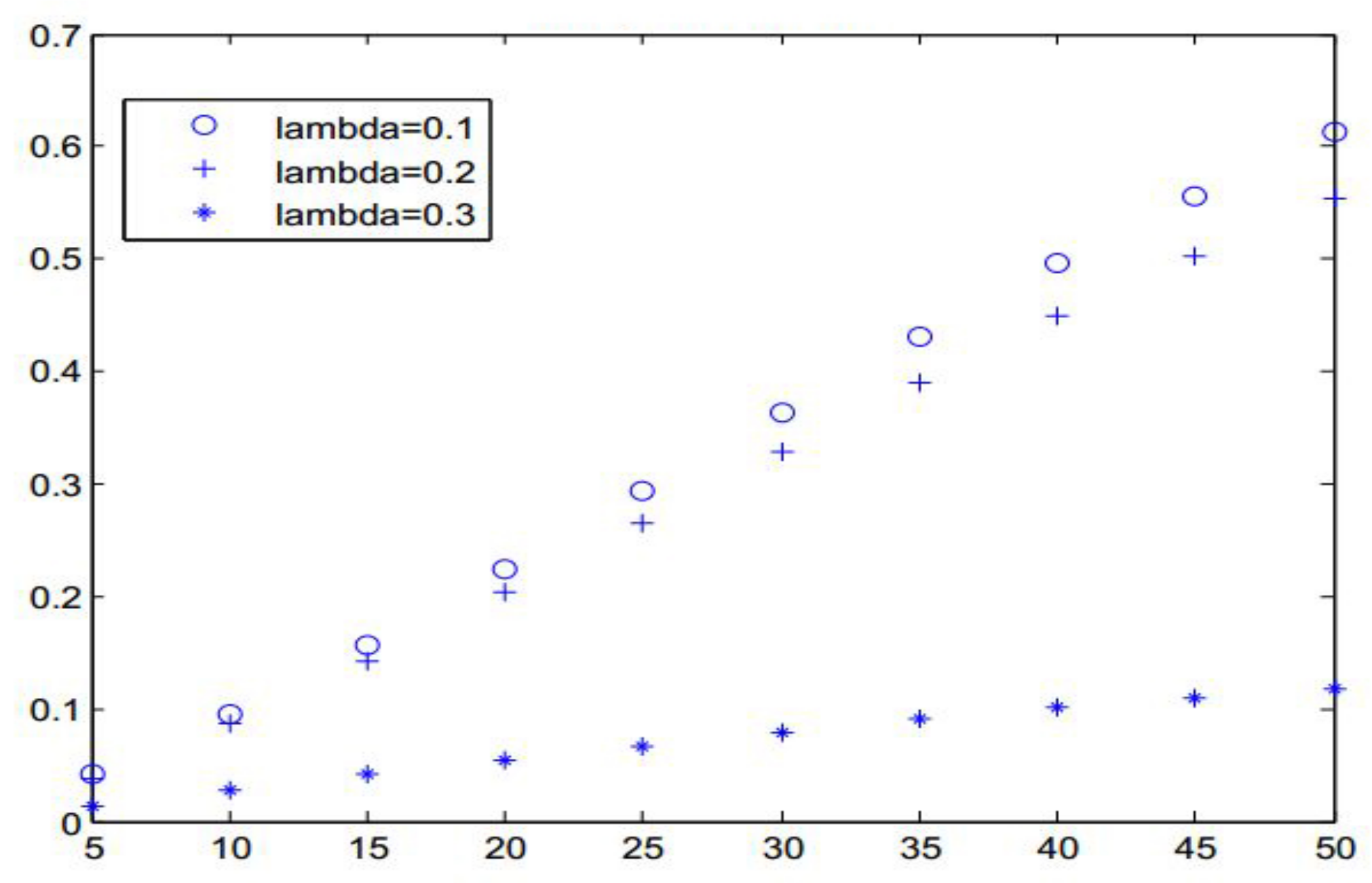
We perturb the value by , where and in order to guarantee the presence of outliers. We calculate the ML estimate of under the perturbed and non-perturbed data, by fitting both data sets under the AR(1) model with , respectively. Then, we compute the relative changes of the estimates as , where is the estimate of under the perturbed data and is the estimate of under the non-perturbed data. The above computation in MATLAB (version 9.3, MathWorks, US) runs five iterations to converge in less than 60 s on a PC. Our experience indicates that the computation runs up to 10 iterations to converge in less than 120 s for even . Figure 1 shows the effectiveness of the influence diagnostics.
4.2. Simulation Study II: Comparing SN and Normal Distributions
We perform a numerical simulation to examine the effectiveness of our method under SN distributions. The results under the SN and normal distributions are compared as follows:
- Step 1. We use the simulated data with perturbed by , where and . We fit an AR(1) model under normality to the data, and obtain the fitted AR(1) model given by where .
- Step 2. We conduct a local influence diagnostic analytics under the normal distribution using the diagnostic results given by [18].
As presented, twenty-four influential observations are detected by the local influence diagnostic analytics under the SN distribution, which is more than the twenty influential values detected by the local influence analytics under the normal distribution. These results are informative and as expected. We see that the influential values (that is, cases #62, #153, #201 and #301) are less than zero.
As we understand, when for the SN distribution is larger than zero, it is easier to find possible influential values less than zero due to the difference in patterns between the SN distribution and the normal distribution. This indicates that the diagnostic results under the SN distribution established in Section 3 work well.
4.3. Real-World Data Analysis
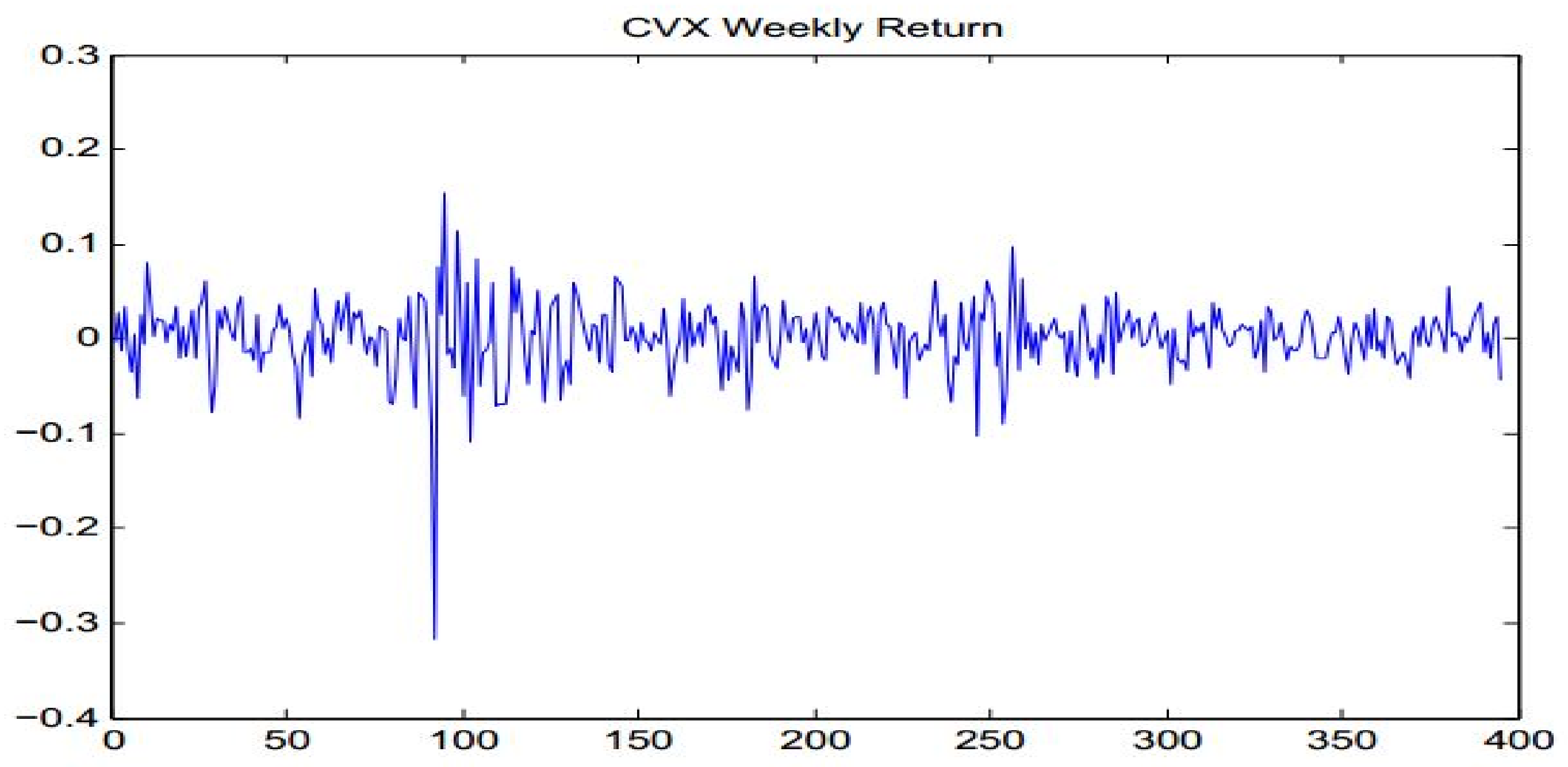
We conduct an empirical example of financial data based on our results presented in Section 2 and Section 3. We choose Chevron shares (hereinafter referred to as CVX weekly financial return data), which were collected from 12 January 2007 to 1 August 2014 to construct the AR models. Figure 3 shows the log transformation of this data set (a total of 395 observations).
We first determine the order of the AR model, using the following steps:
- Step 1. We assume the data are subject to an AR model, for , given by
- Step 2. For the ith equation given in (17), we let be the OLS estimate of , where the superscript denotes the estimates for the AR(i) model. Then, the residual is defined as The estimated variance for the AR(i) model is expressed as .
- Step 3. We use the ith and th equations given in (17) to test versus , that is, we test the AR(i) model versus the AR() model. The test statistic is defined as
For our model, follows an asymptotically chi-square distribution with one degree of freedom, that is, .
We calculate by (18), for , and present the result in Table 2. As the 99th percentile of the chi-square distribution with one degree of freedom is 6.635 ( from Table 2), we select the order of the AR(p) model to be .
From the EM algorithm detailed in Section 2, we can find the estimate of parameter given by
Since the absolute values of , and all are less than 1, we can accept that the CVX time series is stationary for the AR(3) model. Thus, we obtain a predictive model in the fitted SN AR(3) structure given by
with , , and .
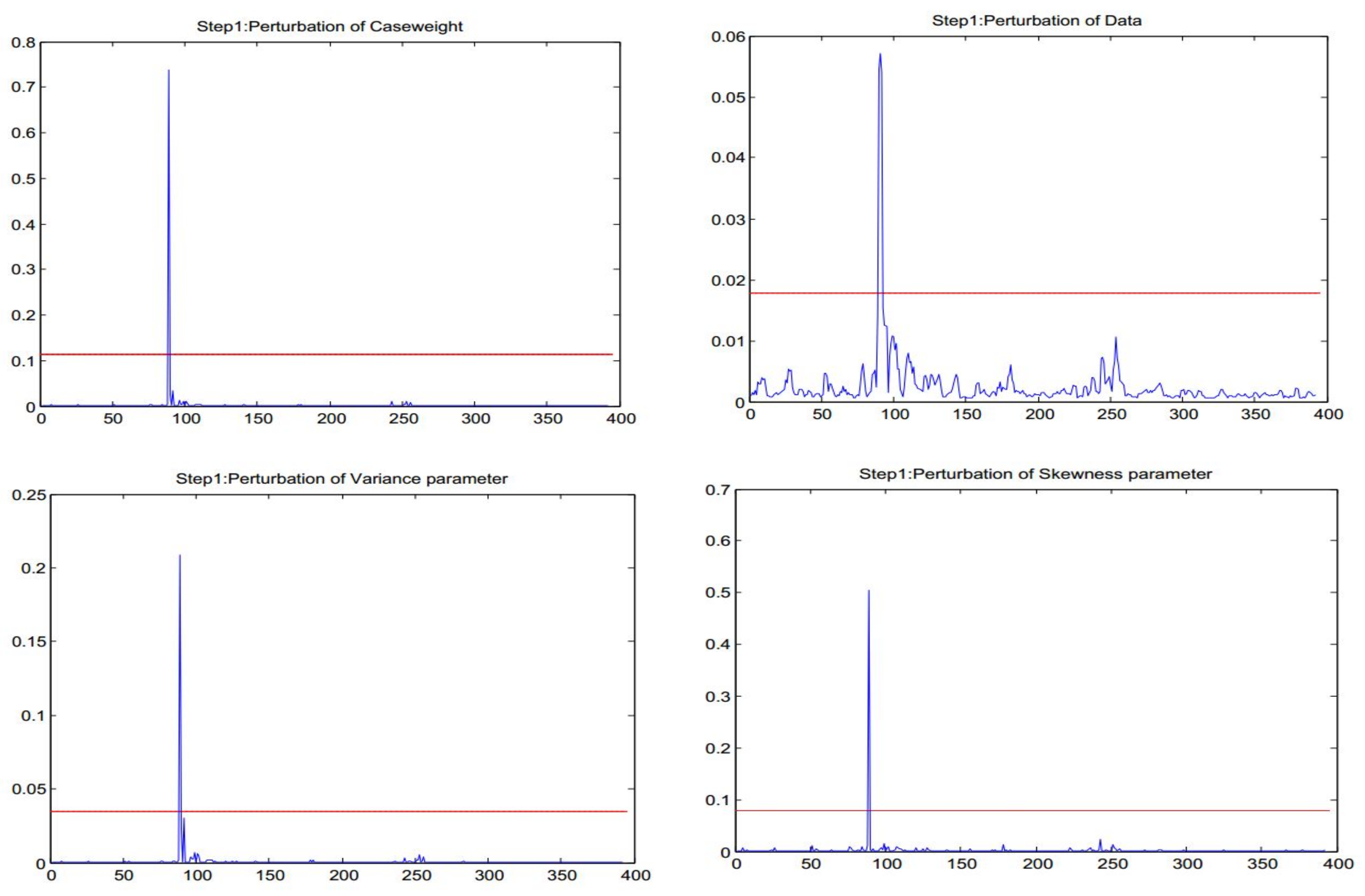
By applying the method in Section 3, we can conduct influence analysis for the SN AR(3) model. After calculating the observed Hessian matrix and the matrices for the four perturbation schemes of case-weights, data, variance parameter, and skewness parameter, we obtain the diagnostics matrices , , , and , respectively. In this case, we select the benchmark as , with the values of 0.1144, 0.0178, 0.0347, and 0.0791 established in the simulation study for the four perturbation schemes, respectively.
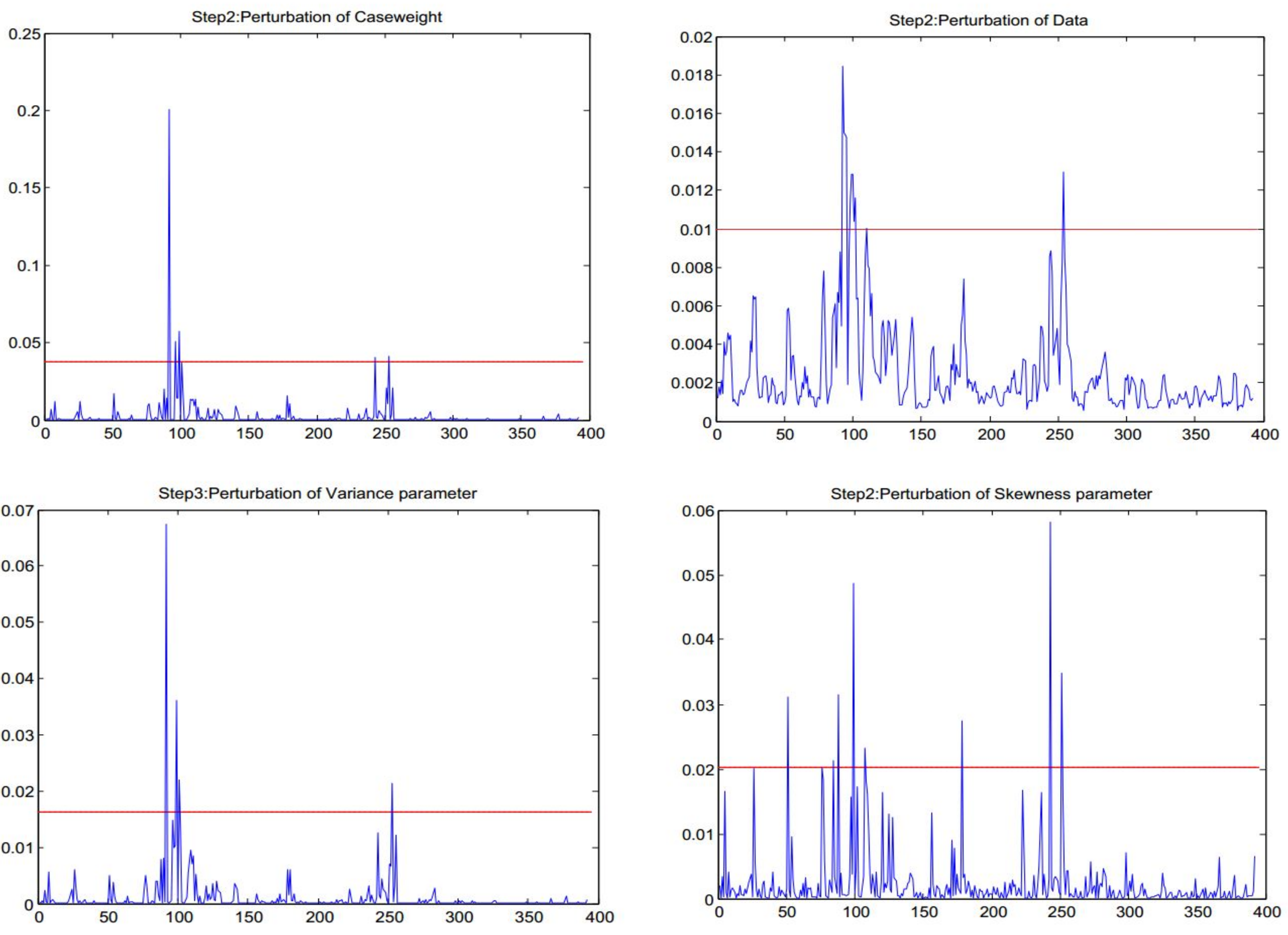
In Figure 4, the straight line represents the benchmark value which determines whether an observation is potentially influential. The observation is justified to be potentially influential when its diagnostic value exceeds the benchmark.
Firstly, we only find case #92 to be potentially influential. The other potential influential observations may be masked by case #92. Similar to a step-wise diagnostic procedure proposed by [6], a second step of identification of influential observations is conducted. In the second rstep, we replace the value of case #92 by the average of cases #91 and #93 to get a new time series.
We re-fit an AR model in the same manner as done previously in the first step. For the new time series, the parameters in the SN AR model are again estimated by applying the EM-algorithm with the order also selected to be three. Thus, we present the new SN AR(3) model as
with , , . Since the absolute values of
, and are all less than one, we can accept the CVX time series to be stationary for the AR(3) model. For the new AR(3) model, we conduct influence analysis. We select the benchmark as again, with the four values of 0.0377, 0.0100, 0.0162, and 0.0203 for the corresponding perturbation schemes, respectively. Thus, twenty-two influence observations are detected in Figure 5, summarized in Table 3. It tallies the observations which are identified to be potentially influential for CVX, and an "*" in Table 3 indicates that the observation has been identified via the assigned perturbation scheme. It is worth noting that the points shown in Table 3 correspond to a number of material historical events. Many of these points relate to events around the 2008 global financial crisis. For example, on September 7 2008, the US Treasury Department announced to take over Fannie Mae and Freddie Mac. On 3 October 2008, the Bush administration signed a total of up to 700 billion dollars in a financial rescue plan. This shows the effectiveness of our procedure in identifying potentially influential observations to improve modeling outcomes.
5. Conclusions
In this paper, we have researched the influence diagnostics in the AR(p) model under skew-normal distributions. We have obtained the normal curvatures for the model under four perturbation schemes, including the newly proposed perturbation of skewness. We have conducted a Monte Carlo simulation study to obtain approximate benchmark values for determining those possible influential points, and use them to analyze the weekly log-returns of Chevron. The findings outlined in this paper suggest that our local influence approach in the AR(p) model effectively identifies potentially influential observations to improve the fit of the model.
Note that we have made a new application of the matrix differential calculus developed by [31] in mathematical optimization and data analysis. In particular, this paper focuses on the detection of local (rather than global) influential observations. The extension of the current study to identify global influential observations will be considered in the future.
Author Contributions
Data curation, Y.L.; formal analysis, G.M. and S.L.; investigation, G.M., V.L. and A.T.; methodology, V.L., S.L. and A.T.; writing–original draft, V.L.; writing–review and editing, S.L. and A.T. All authors have read and agreed to the published version of the manuscript.
Funding
This research was supported partially by grant “Fondecyt 1200525” from the National Commission for Scientific and Technological Research of the Chilean government.
Acknowledgments
The authors would also like to thank the Editor and Reviewers for their constructive comments which led to improve the presentation of the manuscript.
Conflicts of Interest
The authors declare no conflict of interest.
Appendix A
Based on the matrix differential calculus presented by [31], we establish the derivatives involved in our calculations.
Appendix A.1. The Hessian Matrix
For the function , we have
where
The first-order derivatives related to in (7) are given by
The second-order derivatives related to in (7) are given by
Appendix A.2. Perturbation Matrix for Case-Weights
For the function given in (10), we have
The first-order derivatives related to in (11) are given by
The second-order derivatives related to in (11) are given by
Noting that , we obtain (11).
Appendix A.3. Perturbation Matrix for Data
For the function given in (12), we have
The first-order derivatives related to in (13) are given by
The second-order derivatives related to in (13) are given by
Noting that , we obtain (13).
Appendix A.4. Perturbation Matrix for Scale
For the function given in (14), we have
The first-order derivatives related to in (15) are given by
The second-order derivatives related to in (15) are given by
Noting that , we obtain (15).
Appendix A.5. Perturbation Matrix for Skewness
For the function given in (16), we have
The first-order derivatives related to in (16) are given by
The second-order derivatives related to in (16) are given by
Noting that , we obtain (16).
References
- Hyndman, R.J.; Athanasopoulos, G. Forecasting: Principles and Practice; OTexts: Melbourne, Australia, 2018. [Google Scholar]
- Liu, T.; Liu, S.; Shi, L. Time Series Analysis Using SAS Enterprise Guide; Springer: Singapore, 2020. [Google Scholar]
- Li, W.K. Diagnostic Checks in Time Series; Chapman and Hall/CRC: Boca Raton, FL, USA, 2004. [Google Scholar]
- Liu, S.; Welsh, A.H. Regression diagnostics. In International Encyclopedia of Statistical Science; Lovric, M., Ed.; Springer: Berlin/Heidelberg, Germany, 2011; pp. 1206–1208. [Google Scholar]
- Cook, D. Assessment of local influence. J. R. Stat. Soc. B 1986, 48, 133–169. [Google Scholar] [CrossRef]
- Shi, L.; Huang, M. Stepwise local influence analysis. Comput. Stat. Data Anal. 2011, 55, 973–982. [Google Scholar] [CrossRef]
- Lu, J.; Shi, L.; Chen, F. Outlier detection in time series models using local influence method. Comm. Stat. Theor. Meth. 2012, 41, 2202–2220. [Google Scholar] [CrossRef]
- Cao, C.Z.; Lin, J.G.; Shi, J.Q. Diagnostics on nonlinear model with scale mixtures of skew-normal and first-order autoregressive errors. Statistics 2014, 48, 1033–1047. [Google Scholar] [CrossRef]
- Leiva, V.; Liu, S.; Shi, L.; Cysneiros, F.J.A. Diagnostics in elliptical regression models with stochastic restrictions applied to econometrics. J. Appl. Stat. 2016, 43, 627–642. [Google Scholar] [CrossRef]
- Liu, S.; Leiva, V.; Ma, T.; Welsh, A.H. Influence diagnostic analysis in the possibly heteroskedastic linear model with exact restrictions. Stat. Meth. Appl. 2016, 25, 227–249. [Google Scholar] [CrossRef] [Green Version]
- Liu, S.; Ma, T.; SenGupta, A.; Shimizu, K.; Wang, M.Z. Influence diagnostics in possibly asymmetric circular-linear multivariate regression models. Sankhya B 2017, 79, 76–93. [Google Scholar] [CrossRef]
- Garcia-Papani, F.; Leiva, V.; Ruggeri, F.; Uribe-Opazo, M.A. Kriging with external drift in a Birnbaum-Saunders geostatistical model. Stoch. Environ. Res. Risk Assess. 2019, 32, 1517–1530. [Google Scholar] [CrossRef]
- Leao, J.; Leiva, V.; Saulo, H.; Tomazella, V. Incorporation of frailties into a cure rate regression model and its diagnostics and application to melanoma data. Stat. Med. 2018, 37, 4421–4440. [Google Scholar] [CrossRef]
- Tapia, A.; Leiva, V.; Diaz, M.P.; Giampaoli, V. Influence diagnostics in mixed effects logistic regression models. TEST 2019, 28, 920–942. [Google Scholar] [CrossRef]
- Tapia, H.; Giampaoli, V.; Diaz, M.P.; Leiva, V. Sensitivity analysis of longitudinal count responses: A local influence approach and application to medical data. J. Appl. Stat. 2019, 46, 1021–1042. [Google Scholar] [CrossRef]
- Liu, S. On diagnostics in conditionally heteroskedastic time series models under elliptical distributions. J. Appl. Prob. 2004, 41, 393–405. [Google Scholar] [CrossRef]
- Zevallos, M.; Santos, B.; Hotta, L.K. A note on influence diagnostics in AR(1) time series models. J. Stat. Plan. Inference 2012, 142, 2999–3007. [Google Scholar] [CrossRef]
- Liu, Y.; Ji, G.; Liu, S. Influence diagnostics in a vector autoregressive model. J. Stat. Comput. Simul. 2015, 85, 2632–2655. [Google Scholar] [CrossRef]
- Azzalini, A. A class of distribution which includes the normal ones. Scand. J. Stat. 1985, 12, 171–178. [Google Scholar]
- Eling, M. Fitting insurance claims to skewed distributions: Are the skew-normal and skew-student good models? Insur. Math. Econ. 2012, 51, 239–248. [Google Scholar] [CrossRef]
- Azzalini, A. The Skew-Normal and Related Families; Cambridge University Press: Cambridge, UK, 2014. [Google Scholar]
- Arnold, B.C.; Gomez, H.W.; Varela, H.; Vidal, I. Univariate and bivariate models related to the generalized epsilon-skew-Cauchy distribution. Symmetry 2019, 11, 794. [Google Scholar] [CrossRef] [Green Version]
- Cysneiros, F.J.A.; Leiva, V.; Liu, S.; Marchant, C.; Scalco, P. A Cobb-Douglas type model with stochastic restrictions: Formulation, local influence diagnostics and data analytics in economics. Qual. Quant. 2019, 53, 1693–1719. [Google Scholar] [CrossRef]
- Huerta, M.; Leiva, V.; Liu, S.; Rodriguez, M.; Villegas, D. On a partial least squares regression model for asymmetric data with a chemical application in mining. Chem. Intell. Lab. Syst. 2019, 190, 55–68. [Google Scholar] [CrossRef]
- Ventura, M.; Saulo, H.; Leiva, V.; Monsueto, S. Log-symmetric regression models: Information criteria, application to movie business and industry data with economic implications. Appl. Stoch. Models Bus. Ind. 2019, 35, 963–977. [Google Scholar] [CrossRef]
- Maleki, M.; Arellano-Valle, R.V. Maximum a-posteriori estimation of autoregressive processes based on finite mixtures of scale-mixtures of skew-normal distributions. J. Stat. Comput. Simul. 2017, 87, 1061–1083. [Google Scholar] [CrossRef]
- Bolfarine, H.; Montenegro, L.C.; Lachos, V.H. Influence diagnostics for skew-normal linear mixed models. Indian J. Stat. 2007, 69, 648–670. [Google Scholar]
- Xie, F.C.; Lin, J.G.; Wei, B.C. Diagnostics for skew-normal nonlinear regression models with AR(1) errors. Comput. Stat. Data Anal. 2009, 53, 4403–4416. [Google Scholar] [CrossRef]
- Garay, A.M.; Lachos, V.H.; Labra, F.V.; Ortega, E.M.M. Statistical diagnostics for nonlinear regression models based on scale mixtures of skew-normal distributions. J. Stat. Comput. Simul. 2014, 84, 1761–1778. [Google Scholar] [CrossRef]
- Carmichael, B.; Coën, A. Asset pricing with skewed-normal return. Finance Res. Lett. 2013, 10, 50–57. [Google Scholar] [CrossRef]
- Magnus, J.R.; Neudecker, H. Matrix Differential Calculus with Applications in Statistics and Econometrics; Wiley: Chichester, UK, 2019. [Google Scholar]
- Dempster, A.P.; Laird, N.M.; Rubin, D.B. Maximum likelihood from incomplete data via the EM algorithm. J. R. Stat. Soc. B 1977, 39, 1–38. [Google Scholar]
- McLachlan, G.; Krishnan, T. The EM Algorithm and Extensions; Wiley: New York, NY, USA, 1997. [Google Scholar]
- Poon, W.Y.; Poon, Y.S. Conformal normal curvature and assessment of local influence. J. R. Stat. Soc. B 1999, 61, 51–61. [Google Scholar] [CrossRef]
Figure 1.
Relative change of estimate of against d.

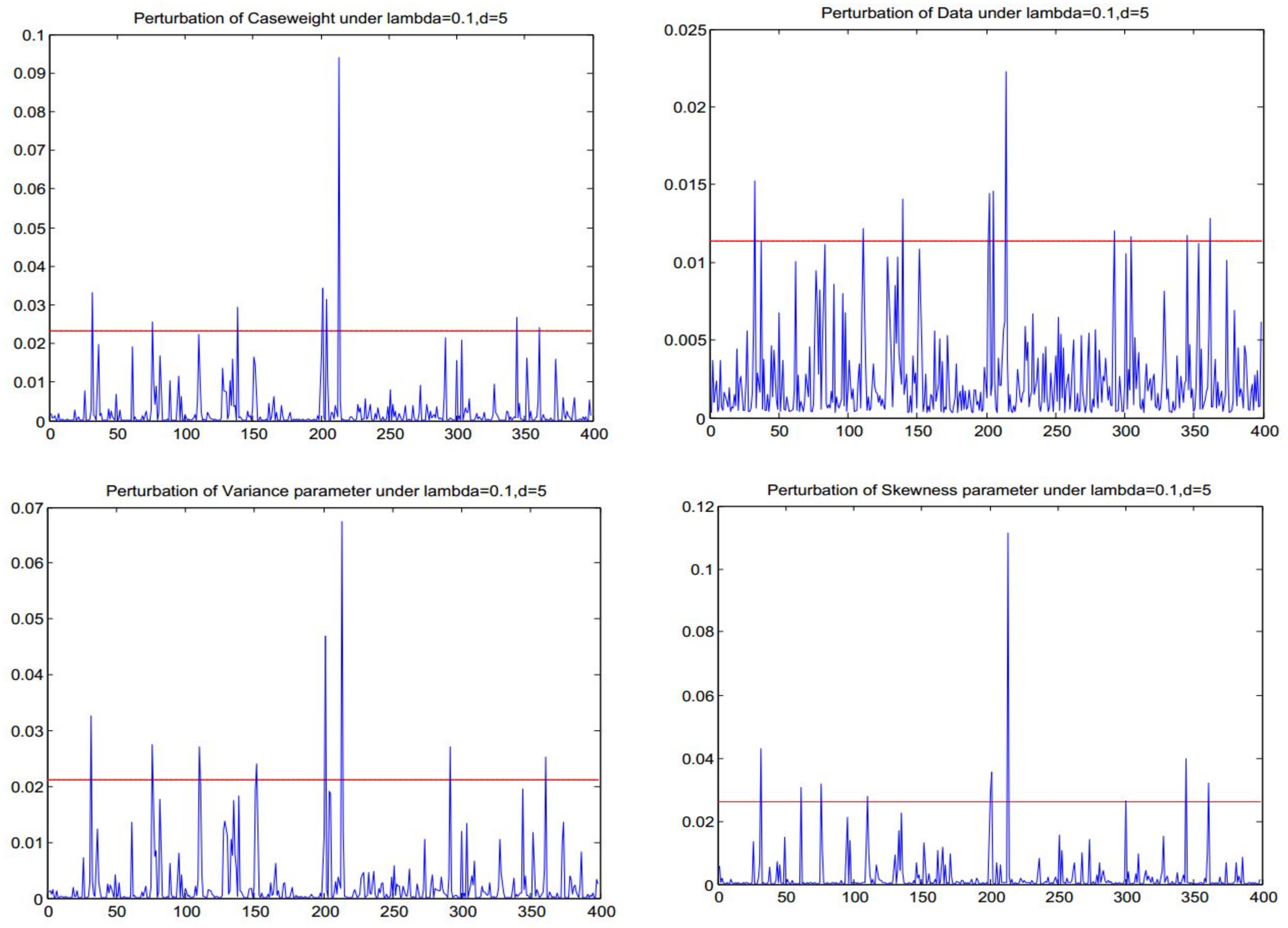
Figure 2.
Diagnostics for the perturbations of case-weights, data, variance and skewness.

Figure 3.
CVX weekly log-returns.

Figure 4.
Diagnostics for the perturbations of case-weights, data, variance, and skewness in the SN AR(3) model [step 1].
Figure 4.
Diagnostics for the perturbations of case-weights, data, variance, and skewness in the SN AR(3) model [step 1].

Figure 5.
Diagnostics for the perturbations of case-weights, data, variance, and skewness in the SN AR(3) model [step 2].
Figure 5.
Diagnostics for the perturbations of case-weights, data, variance, and skewness in the SN AR(3) model [step 2].


Table 1.
Local influence results for normal and SN models.
| ID | Index under the Normal Model | Index under the SN Model | Observed Value |
|---|---|---|---|
| 1 | 33 | 33 | −0.334 |
| 2 | 34 | 34 | 0.030 |
| 3 | - | 62 | −0.271 |
| 4 | 77 | 77 | −0.260 |
| 5 | 111 | 111 | −0.297 |
| 6 | 112 | 112 | −0.225 |
| 7 | 140 | 140 | 0.319 |
| 8 | 141 | 141 | 0.089 |
| 9 | - | 153 | −0.175 |
| 10 | - | 201 | −0.269 |
| 11 | 202 | 202 | −0.326 |
| 12 | 203 | 203 | −0.090 |
| 13 | 205 | 205 | 0.328 |
| 14 | 206 | 206 | −0.124 |
| 15 | 214 | 214 | −0.406 |
| 16 | 215 | 215 | −0.159 |
| 17 | 293 | 293 | 0.296 |
| 18 | 294 | 294 | −0.012 |
| 19 | - | 301 | −0.278 |
| 20 | 306 | 306 | 0.043 |
| 21 | 345 | 345 | −0.293 |
| 22 | 346 | 346 | −0.092 |
| 23 | 362 | 362 | −0.307 |
| 24 | 363 | 363 | −0.048 |
Table 2.
Test statistic , for using CVX data.
| Order | 1 | 2 | 3 | 4 | 5 | 6 | 7 |
|---|---|---|---|---|---|---|---|
| −0.3826 | −1.001 | 16.9551 | 2.9495 | −1.6675 | −1.9619 | 8.9958 |
Table 3.
Summary of the curvature-based diagnostic analytics.
| ID | Time | CVXs Return | Case-Weights | Data | Variance | Skewness |
|---|---|---|---|---|---|---|
| 54 | 2008-01-18 | −8.286% | * | |||
| 79 | 2008-07-11 | −6.687% | * | |||
| 87 | 2008-09-05 | −7.329% | * | |||
| 91 | 2008-10-03 | −9.109% | * | |||
| 92 | 2008-10-10 | −31.674% | * | * | * | * |
| 95 | 2008-10-31 | 15.4665% | * | * | ||
| 96 | 2008-11-07 | −1.54% | * | |||
| 97 | 2008-11-14 | −1.067% | * | |||
| 98 | 2008-11-21 | −3.06% | * | |||
| 99 | 2008-11-28 | 11.4104% | * | |||
| 101 | 2008-12-12 | 5.9723% | * | |||
| 102 | 2008-12-19 | −10.888% | * | * | * | * |
| 103 | 2008-12-26 | −0.708% | * | |||
| 104 | 2009-01-02 | 8.4069% | * | |||
| 105 | 2009-01-09 | −4.956% | * | * | ||
| 110 | 2009-02-13 | −7.152% | * | |||
| 113 | 2009-03-06 | −4.102% | * | |||
| 181 | 2010-06-25 | −7.505% | * | |||
| 246 | 2011-09-23 | −10.154% | * | * | ||
| 254 | 2011-11-18 | −8.955% | * | |||
| 256 | 2011-12-02 | 9.6993% | * | |||
| 257 | 2011-12-09 | 2.4863% | * |
© 2020 by the authors. Licensee MDPI, Basel, Switzerland. This article is an open access article distributed under the terms and conditions of the Creative Commons Attribution (CC BY) license (http://creativecommons.org/licenses/by/4.0/).
Share and Cite
MDPI and ACS Style
Liu, Y.; Mao, G.; Leiva, V.; Liu, S.; Tapia, A. Diagnostic Analytics for an Autoregressive Model under the Skew-Normal Distribution. Mathematics 2020, 8, 693. https://0-doi-org.brum.beds.ac.uk/10.3390/math8050693
AMA Style
Liu Y, Mao G, Leiva V, Liu S, Tapia A. Diagnostic Analytics for an Autoregressive Model under the Skew-Normal Distribution. Mathematics. 2020; 8(5):693. https://0-doi-org.brum.beds.ac.uk/10.3390/math8050693
Chicago/Turabian StyleLiu, Yonghui, Guohua Mao, Víctor Leiva, Shuangzhe Liu, and Alejandra Tapia. 2020. "Diagnostic Analytics for an Autoregressive Model under the Skew-Normal Distribution" Mathematics 8, no. 5: 693. https://0-doi-org.brum.beds.ac.uk/10.3390/math8050693
Note that from the first issue of 2016, this journal uses article numbers instead of page numbers. See further details here.