A Second-Order Well-Balanced Finite Volume Scheme for the Multilayer Shallow Water Model with Variable Density

Abstract

In this work, we consider a multilayer shallow water model with variable density. It consists of a system of hyperbolic equations with non-conservative products that takes into account the pressure variations due to density fluctuations in a stratified fluid. A second-order finite volume method that combines a hydrostatic reconstruction technique with a MUSCL second order reconstruction operator is developed. The scheme is well-balanced for the lake-at-rest steady state solutions. Additionally, hints on how to preserve a general class of stationary solutions corresponding to a stratified density profile are also provided. Some numerical results are presented, including validation with laboratory data that show the efficiency and accuracy of the approach introduced here. Finally, a comparison between two different parallelization strategies on GPU is presented.

1. Introduction

Shallow-water (or Saint–Venant) type systems are among the most widely used models to study geophysical flows (see [1,2]). However, these types of models have a main limitation or drawback: the consideration of an averaged horizontal velocity while neglecting the vertical components. In order to overcome this limitation, multilayer shallow water models have been developed in recent years. This multilayer approach allows for capturing complex vertical effects and profiles that single layer shallow water models cannot (see [3,4,5]). These multilayer models have been applied by several authors for different geophysical problems, like tsunamis ([6,7,8,9,10]), flooding events ([11,12,13,14,15]), or storm-surges ([16,17,18]).

One possible approach to introduce multilayer shallow water models is the one described by Audusse et al. in [19]. There, the domain is discretized in the vertical direction with an a priori arbitrary number of layers. In each layer, similar assumptions as in the classical shallow water framework are made: the velocity is averaged in the vertical direction, vertical effects are neglected, and the pressure is assumed hydrostatic. In order to allow mass and momentum exchange between layers, an approximation of the vertical flux in the layer is incorporated into the model through non-conservative terms (see [20,21] or [4]). In this way, we are able to obtain a detailed vertical profile of the velocity. Recent developments in multilayer shallow water models concern the local change of the number of layers according to the presence of relevant vertical effects (see [22]).

Another approach to capture complex vertical profiles, but avoiding fully 3D models while calculating the free surface directly, are the so-called $\sigma$-coordinate models ([23]). In those models, as in the multilayer approach, the free surface is defined as a function of the horizontal coordinates. In this way, the free surface is always located at the upper boundary and can be derived from the standard free surface conditions. This simplification provides a new set of models that allows turbulence, solute transport, and also short wave propagation (see [24,25,26]).

A further step in the development of the multilayer shallow-water models is given by the derivation of multilayer shallow water models with non-hydrostatic pressure (see [27,28] or [29]). These models include effects due to the vertical acceleration of the fluid that are derived from the Boussinesq-type wave equations. By doing so, the dispersive properties of the model are enhanced and simulation of more physical effects becomes possible at the cost of a greater computational effort.

While multilayer shallow-water models can satisfactorily capture vertical stratification due to velocity, they fail to provide an adequate solution when the stratification is due to general changes in density, like the ones due to variations in temperature and/or salinity. The examples of density driven currents in natural geophysical flows are numerous. One classical example is at the Strait of Gibraltar, where two currents, one from the Atlantic Ocean and the other from the Mediterranean Sea, meet. These two flows are different in terms of temperature and salinity. The water from the Mediterranean sea has more salinity due to greater evaporation. Thus, the Mediterranean flow is denser and tends to flow under the current from the Atlantic Ocean. Capturing the vertical profile in this situation is impossible for standard shallow water equations, and it is necessary to apply a model that takes into account these buoyancy effects.

In this framework, several authors have proposed multilayer shallow water models with variable density. In [30,31], for instance, the differences in density are due to suspended sediment. In [32], the authors propose a multilayer shallow water model that takes into account density variations due to a given tracer such as the temperature.

Here, we shall consider a similar model to the one presented in [32]. The main differences concern the derivation, where we propose a slightly different approximation of the exchange terms between layers, and especially in the numerical discretization of the model. Moreover, we also propose a parallel implementation on GPUs.

The model considered is quite different from other approximations that assume immiscible layers (see [33,34]) or consider the water entrainment as an heuristic-dependent source term (see [35]). Here, we allow the density variations to circulate freely between the layers. Let us remark that the layers are just a means of capturing a complex vertical profile and do not correspond to physical layers.

Concerning the numerical approximation of shallow water type models, a relevant issue is the exact preservation of some equilibrium states. In particular, in the simulation of geophysical flows, an important problem consists of a perturbation of these equilibrium states. The design of numerical schemes that are well-balanced, that is, that preserve the stationary solutions of the model exactly, is of great importance for the long-term numerical stability of the simulation. The exact preservation of these stationary solutions, especially for the shallow water equations, is a relevant research topic (see [36,37,38], or [39], and the references therein ).

In this work, we propose a path-conservative numerical scheme based on a modified hydrostatic reconstruction ([40]) combined with a second order reconstruction procedure. The well-balanced properties of the scheme are also discussed.

The paper is organized as follows. In Section 2, we describe the governing equations of the problem, we provide a general formulation for the multilayer approach, we give the general expression of the multilayer model and we present some relevant stationary solutions. Section 3 is dedicated to introduce the second-order numerical scheme used to discretize the multilayer system. The proposed numerical scheme is a well-balanced path-conservative second order numerical scheme based on a modified hydrostatic reconstruction. Moreover, hints on how to preserve a general class of stationary solutions corresponding to a stratified density profile are also given. In Section 4, we present some numerical tests, including comparison between the model and a laboratory experiment. Section 5 summarizes some conclusions. Finally, in Appendix A, a study of performance and computational cost for different parallelization strategies is addressed and in Appendix B, a thorough description of the model derivation is provided.

2. Governing Equations and Model

The free surface Navier–Stokes equation in a d-dimensional space ($d=2,3$) are considered. We denote by $\mathit{v}=(\mathit{u},w)$ the velocity function with $\mathit{u}\in {\mathbb{R}}^{d-1}$ the horizontal components of the velocity and w the vertical one. We will consider two continuity equations: one corresponding to an incompressible flow with constant density ${\rho }_0$ and the other corresponding to the advected flow with variable density, $\rho$,

$$\begin{array}{ccc}\hfill \nabla ·\mathit{v}& =& 0,\hfill \\ \hfill {\partial }_t\rho +\nabla ·\left(\rho \mathit{v}\right)& =& 0,\hfill \\ \hfill {\partial }_t\left(\rho \mathit{v}\right)+\nabla ·(\rho \mathit{v}\otimes \mathit{v})& =& -g\rho \mathit{k}+\nabla ·\Sigma ,\hfill \end{array}$$

(1)

where $\mathit{k}={(\mathbf{0},1)}^T$, g is the constant gravity function, $\rho$ is the total density of the fluid, and the total stress tensor is given by $\Sigma =-p\mathit{I}+\mathit{T}$, with $\mathit{I}$ the identity tensor, p the pressure term, and $\mathit{T}$ the tensor corresponding to the viscous terms,

$$\mathit{T}=\left(\begin{array}{cc}{\mathit{T}}_{\mathit{H}}& T_{xz}\\ T_{xz}^{\prime }& T_{zz}\end{array}\right).$$

(2)

We shall decompose the total density $\rho$ as the sum of a reference density, denoted by ${\rho }_0,$ and the corresponding variation from that reference density, denoted by ${\rho }_1$,

$$\rho ={\rho }_0+{\rho }_1.$$

(3)

If we now divide (1) by ${\rho }_0$, we obtain the following system:

$$\begin{array}{ccc}\hfill \nabla ·\mathit{v}& =& 0,\hfill \\ \hfill {\partial }_t\left(\theta \right)+\nabla ·\left(\theta \mathit{v}\right)& =& 0,\hfill \\ \hfill {\partial }_t\left(\theta \mathit{v}\right)+\nabla ·(\theta \mathit{v}\otimes \mathit{v})& =& -g\theta \mathit{k}+\frac{1}{{\rho }_0}\nabla ·\Sigma ,\hfill \end{array}$$

(4)

with

$$\theta =\frac{\rho }{{\rho }_0}=1+\frac{{\rho }_1}{{\rho }_0}.$$

(5)

We shall now consider a multilayer shallow water approach to system (4). In the multilayer approach, the fluid domain ${\mathsf{\Omega }}_F\left(t\right)$ is divided along the vertical dimension into a set of $M\in {\mathbb{N}}^{\ast }$ layers of thickness $h_{\alpha }(t,x)$ with $M+1$ smooth interfaces ${\mathsf{\Gamma }}_{\alpha +\frac{1}{2}}\left(t\right),$ which shall be described as (see Figure 1):

$${\mathsf{\Gamma }}_{\alpha +\frac{1}{2}}\left(t\right)=\left\{(\mathit{x},z)\in {\mathsf{\Omega }}_F\left(t\right),\mathrm{such}\mathrm{that}z=z_{\alpha +\frac{1}{2}}(t,\mathit{x})\right\},\alpha =0,1,\dots ,M.$$

The layers will be then described as

$${\mathsf{\Omega }}_{\alpha }\left(t\right)=\left\{(\mathit{x},z)\in {\mathsf{\Omega }}_F\left(t\right),\mathrm{such}\mathrm{that}{z}_{\alpha -\frac{1}{2}}(t,\mathit{x})<z<z_{\alpha +\frac{1}{2}}(t,\mathit{x})\right\},\alpha =1,\dots ,M.$$

We shall denote by $z_B=z_{\frac{1}{2}}$ and $z_S=z_{M+\frac{1}{2}}$ the bottom and the free-surface, respectively. Let us define $h_{\alpha }=z_{\alpha +\frac{1}{2}}-z_{\alpha -\frac{1}{2}}$ as the thickness of each layer. The total height of the fluid column is then given by ${\displaystyle h=z_S-z_B={\displaystyle \sum _{\alpha =1}^M}{h}_{\alpha }}$.

Following the usual approach in multilayer shallow water models, we consider the horizontal velocity and relative density fluctuations to be independent of the vertical variable z:

$${\mathit{v}}_{|{\mathsf{\Omega }}_{\alpha }\left(t\right)}:={\mathit{v}}_{\alpha }:={({\mathit{u}}_{\alpha },w_{\alpha })}^{\prime },{\theta }_{|{\mathsf{\Omega }}_{\alpha }}:={\theta }_{\alpha },p_{|{\mathsf{\Omega }}_{\alpha }}:=p_{\alpha },$$

where ${\mathit{u}}_{\alpha }$ is the horizontal velocity and $w_{\alpha }$ is the vertical one. We also assume that both $w_{\alpha }$ and $p_{\alpha }$ are linear in z inside each layer. Moreover, we suppose that pressure is also continuous at the interfaces and hydrostatic pressure is assumed, so that

$$p_{\alpha }(t,x,z)=p_{\alpha +\frac{1}{2}}+{\theta }_{\alpha }g(z_{\alpha +\frac{1}{2}}-z),$$

(6)

with

$$p_{\alpha +\frac{1}{2}}(t,x)=p_S(t,x)+g{\displaystyle \sum _{\beta =\alpha +1}^M}{\theta }_{\beta }{h}_{\beta }(t,x).$$

(7)

Here, the component $p_{\alpha +\frac{1}{2}}$ is the hydrostatic pressure at ${\mathsf{\Gamma }}_{\alpha +\frac{1}{2}}\left(t\right)$ and $p_S$ denotes the pressure at the free surface. Therefore, the unknowns of the system are the depths of the layers, the density fluctuation, and the horizontal velocities in each layer. Remark that ${\partial }_z{w}_{\alpha }=-\nabla ·{\mathit{u}}_{\alpha }$ and therefore it is not considered as an unknown. As it is usual in multilayer shallow water type systems, we shall consider $l_{\alpha }\in (0,1),\alpha =1,\dots ,M$ such that ${\displaystyle {\displaystyle \sum _{\alpha =1}^M}{l}_{\alpha }=1.}$ Then, the layer thickness is assumed to be proportional to the total depth, so that $h_{\alpha }=l_{\alpha }h$.

There is no hope for such a particular set $\left({\mathit{v}}_{\alpha },{\theta }_{\alpha },p_{\alpha }\right)$ to be a solution of the complete equations in the layer ${\mathsf{\Omega }}_{\alpha }\left(t\right)$. Instead, we shall consider a reduced weak formulation with particular test functions. A detailed derivation of the vertical integration procedure can be found in [20,30], or [4]. A thorough derivation of this specific model is given in Appendix B. For the sake of simplicity, from now on, we will suppose $d=2$ and merely present the final version of the model, where the horizontal viscosity terms have been neglected

$$\{\begin{array}{c}{\partial }_{t}h+{\partial }_x\left(h{\displaystyle \sum _{\beta =1}^M}{l}_{\beta }{u}_{\beta }\right)=0,\hfill \\ {\partial }_t\left(h{\theta }_{\alpha }\right)+{\partial }_x\left(h{\theta }_{\alpha }{u}_{\alpha }\right)=\frac{1}{l_{\alpha }}\left({\theta }_{\alpha +\frac{1}{2}}{G}_{\alpha +\frac{1}{2}}-{\theta }_{\alpha -\frac{1}{2}}{G}_{\alpha -\frac{1}{2}}\right),\hfill \\ {\partial }_t\left(h{\theta }_{\alpha }{u}_{\alpha }\right)+{\partial }_x\left(h{\theta }_{\alpha }{u}_{\alpha }^2\right)+gh{\theta }_{\alpha }{\partial }_x\eta \hfill \\ +gh\left({\displaystyle \sum _{\beta =\alpha +1}^M}{l}_{\beta }({\theta }_{\beta }-{\theta }_{\alpha }){\partial }_{x}h\right)+gh{\displaystyle \sum _{\beta =\alpha +1}^M}{l}_{\beta }h{\partial }_x{\theta }_{\beta }+\frac{1}{2}g{l}_{\alpha }{h}^2{\partial }_x{\theta }_{\alpha }\hfill \\ =\frac{1}{l_{\alpha }}\left(u_{\alpha +\frac{1}{2}}{\theta }_{\alpha +\frac{1}{2}}{G}_{\alpha +\frac{1}{2}}-u_{\alpha -\frac{1}{2}}{\theta }_{\alpha -\frac{1}{2}}{G}_{\alpha -\frac{1}{2}}\right),\hfill \end{array}$$

(8)

where $\eta =h+b$ is the free surface and $G_{\alpha \pm \frac{1}{2}}$$\alpha =1,\dots ,M-1$, are the mass exchange terms between layers, defined by

$$G_{\alpha +\frac{1}{2}}={\displaystyle \sum _{\beta =1}^{\alpha }}{l}_{\beta }\left({\partial }_{t}h+{\partial }_x\left(h{u}_{\beta }\right)\right)={\displaystyle \sum _{\beta =1}^{\alpha }}{l}_{\beta }\left({\partial }_x\left(h{u}_{\beta }\right)-{\partial }_x\left(h{\displaystyle \sum _{\gamma =1}^M}{l}_{\gamma }{u}_{\gamma }\right)\right).$$

(9)

We will also consider no mass exchange at the bottom and the free surface, that is, $G_{\frac{1}{2}}=G_{M+\frac{1}{2}}=0$. In addition, ${\theta }_{\alpha +\frac{1}{2}}$ and $u_{\alpha +\frac{1}{2}}$ are some approximation of u and $\theta$ at the interfaces ${\mathsf{\Gamma }}_{\alpha +\frac{1}{2}}$, $\alpha =1,\dots ,M-1$. Typically,

$$u_{\alpha +\frac{1}{2}}=\frac{u_{\alpha +1}+u_{\alpha }}{2},{\theta }_{\alpha +\frac{1}{2}}=\frac{{\theta }_{\alpha +1}+{\theta }_{\alpha }}{2},\alpha =1,\dots ,M-1,$$

with $u_{\frac{1}{2}}=u_1$, $u_{M+\frac{1}{2}}=u_M$ and ${\theta }_{\frac{1}{2}}={\theta }_1$, ${\theta }_{M+\frac{1}{2}}={\theta }_M$.

System (8) may be rewritten in the following form:

$$\{\begin{array}{c}{\partial }_{t}h+{\partial }_x\left(h{\displaystyle \sum _{\beta =1}^M}{l}_{\beta }{u}_{\beta }\right)=0,\hfill \\ {\partial }_t\left(h{\theta }_{\alpha }\right)+{\partial }_x\left(h{\theta }_{\alpha }{u}_{\alpha }\right)=\frac{1}{l_{\alpha }}\left({\theta }_{\alpha +\frac{1}{2}}{G}_{\alpha +\frac{1}{2}}-{\theta }_{\alpha -\frac{1}{2}}{G}_{\alpha -\frac{1}{2}}\right),\hfill \\ {\partial }_t\left(h{\theta }_{\alpha }{u}_{\alpha }\right)+{\partial }_x\left(h{\theta }_{\alpha }{u}_{\alpha }^2\right)+gh{\theta }_{\alpha }{\partial }_x\eta +\frac{g{l}_{\alpha }}{2}\left(h{\partial }_x\left(h{\theta }_{\alpha }\right)-h{\theta }_{\alpha }{\partial }_{x}h\right)\hfill \\ +g{\displaystyle \sum _{\beta =\alpha +1}^M}{l}_{\beta }\left(h{\partial }_x\left(h{\theta }_{\beta }\right)-h{\theta }_{\alpha }{\partial }_{x}h\right)=\frac{1}{l_{\alpha }}\left(u_{\alpha +\frac{1}{2}}{\theta }_{\alpha +\frac{1}{2}}{G}_{\alpha +\frac{1}{2}}-u_{\alpha -\frac{1}{2}}{\theta }_{\alpha -\frac{1}{2}}{G}_{\alpha -\frac{1}{2}}\right).\hfill \end{array}$$

(10)

Note that pressure terms have been rewritten and reduce to

$$\begin{array}{cc}{P}_{\alpha }:=g\frac{l_{\alpha }}{2}{\partial }_x\left(h^2{\theta }_{\alpha }\right)+h{\partial }_x{p}_{\alpha +\frac{1}{2}}+gh{\theta }_{\alpha }{\partial }_x{z}_{\alpha -\frac{1}{2}}\hfill & \\ & \hfill =gh{\theta }_{\alpha }{\partial }_x\eta +\frac{g{l}_{\alpha }}{2}\left(h{\partial }_x\left(h{\theta }_{\alpha }\right)-h{\theta }_{\alpha }{\partial }_{x}h\right)+g{\displaystyle \sum _{\beta =\alpha +1}^M}{l}_{\beta }\left(h{\partial }_x\left(h{\theta }_{\beta }\right)-h{\theta }_{\alpha }{\partial }_{x}h\right).\end{array}$$

One can easily check that system (10) has non-trivial stationary solutions. Here, we are interested in the particular stationary solutions that satisfy $u_{\alpha }=0$, $\alpha =1,\dots ,M.$ For this particular case, one can distinguish two families of stationary solutions: the one corresponding to the choice of a constant relative density function ${\theta }_{\alpha }=K$, $\alpha =1,\dots ,M$, and the more general case where ${\theta }_{\alpha }$ is not constant.

In the first case, the stationary solution reduces to the well-known lake-at-rest stationary solutions, characterized in this case by

$$u_{\alpha }=0,{\theta }_{\alpha }=K_1,\eta =h+b=K_2,$$

(11)

where $K_1\ge 1$ and $K_2$ are two given constants.

For the second more general case, we shall consider smooth stationary solutions. Then, given two known smooth functions $b\left(x\right)$ and $h\left(x\right)\ge 0$, the stationary solutions are characterized as the regular solutions of the following ODE system:

$$\frac{l_{\alpha }}{2}{\left({\theta }_{\alpha }\right)}^{\prime }+{\displaystyle \sum _{\beta =\alpha +1}^M}{l}_{\beta }{\left({\theta }_{\beta }\right)}^{\prime }=-\frac{1}{h}\left({\theta }_{\alpha }{(h+b)}^{\prime }+{\displaystyle \sum _{\beta =\alpha +1}^M}{l}_{\beta }({\theta }_{\beta }-{\theta }_{\alpha })h^{\prime }\right),\alpha =1,\dots ,M.$$

(12)

Note that the ODE (12) can be solved by an iterative procedure: starting from $\alpha =M$, where the equation only depends on ${\theta }_M$,

$${\left({\theta }_M\right)}^{\prime }=\frac{2}{h{l}_M}{(h+b)}^{\prime }{\theta }_M,$$

and then continue to solve downwards on $\alpha$ so that once that ${\theta }_M,{\theta }_{M-1},\dots ,{\theta }_{\alpha +1}$ have been calculated, (12) corresponds to a scalar ODE for ${\theta }_{\alpha }$ that may be solved.

Note that there exists a trivial class of stationary solutions for the original system (4), which corresponds to a stratified fluid with constant free surface, that is,

$$u=0,\eta \left(x\right)=b\left(x\right)+h\left(x\right)=K,\theta \left(z\right)={\theta }_{surface}+\alpha (\eta -z).$$

(13)

Unfortunately, these types of solutions are not an exact solution of (12). Therefore, they are not stationary solutions for the multilayer system (10), except for the case of constant bottom $b\left(x\right)=cst$. This is due to the particular choice of the vertical discretization used in the multilayer approach. The layers are proportional to the total thickness and the variables have been averaged inside the layer. As a result, averaging of stratified solutions does not result in a stratified solution (space independent of $\theta$) for the multilayer system, unless the bottom and free surface are constant.

Nevertheless, stationary stratified solutions (13) may be approximated in the multilayer framework by the following set of stationary solutions:

$$\begin{array}{c}{u}_{\alpha }=0,\eta \left(x\right)=b\left(x\right)+h\left(x\right)=K,\\ {\theta }_M\left(x\right)={\overline{\theta }}_M\ge 1,\\ {\displaystyle {\theta }_{\alpha }\left(x\right)={\overline{\theta }}_{\alpha }{h}^{2(M-\alpha )}\left(x\right)+{\displaystyle \sum _{\beta =\alpha +1}^M}{S}_{2(M-\beta )}(M-\alpha +1){\overline{\theta }}_{\beta }{h}^{2(M-\beta )}\left(x\right),}\end{array}$$

(14)

with

$$\begin{array}{ccc}\hfill S_{\beta }\left(\alpha \right)& =& (\beta +1)·A_{\frac{\beta +2}{2}+1}\left(\alpha \right)\hfill \\ \hfill A_p\left(k\right)& =& \left\{\begin{array}{cc}1\hfill & \mathrm{if}p\ge k,\hfill \\ (p-1){\displaystyle {\prod }_{\gamma =2}^{k-p}}(1+(p-2)C_{\gamma })\hfill & \mathrm{if}p<k,\hfill \end{array}\right.\hfill \\ \hfill C_{\gamma }& =& C_{\gamma -1}-\frac{1}{Q_{\gamma }}\hfill \\ \hfill Q_{\gamma }& =& Q_{\gamma -1}+i+1\hfill \\ \hfill C_0& =& Q_0=1\hfill \end{array}$$

Here, ${\overline{\theta }}_{\alpha }$ are given constants that should be properly chosen to determine a physical stable solution.

The stationary solutions (14) have been obtained from (12) by the iterative procedure described before.

Figure 2 and Figure 3 show a particular realization of these types of stationary solutions. In particular, we see the vertical distribution of ${\theta }_{\alpha }\left(x\right)$, $\alpha =1,\dots ,M$, along a given channel for the values $M=5$, $M=10$, $M=50$, and $M=100$. We see from the pictures that (14) converges to (13) as $M\to +\infty$.

The study of the hyperbolicity of the proposed model (10) is not an easy task. The model is hyperbolic for the case $M=1$ but remains an open question in general. Nevertheless, numerical simulations show that the eigenvalues of the system are real. It is possible to give an upper and lower bound for the largest and smallest wave speed, ${\lambda }_{max}$, ${\lambda }_{min},$ respectively. Following [31], the minimum and maximum of the wave speeds are bounded by:

$${\lambda }_{min}\ge \overline{u}-\mathsf{\Psi },{\lambda }_{max}\le \overline{u}+\mathsf{\Psi }$$

(15)

where

$$\mathsf{\Psi }=\sqrt{\frac{2M-1}{2M}\left(2{\displaystyle \sum _{\alpha =1}^M}{(\overline{u}-u_{\alpha })}^2+gh\left(1+\frac{1}{M}{\displaystyle \sum _{\beta =1}^M}(2\beta -1){\theta }_{\beta }\right)\right)},$$

(16)

and

$$\overline{u}=\frac{1}{M}{\displaystyle \sum _{\alpha =1}^M}{u}_{\alpha }.$$

(17)

3. Numerical Scheme

The full system (10) can be written in the form of an hyperbolic system with conservative fluxes and non-conservative products as follows:

$${\partial }_t\mathit{w}+{\partial }_x{\mathit{F}}_C\left(\mathit{w}\right)+\mathit{P}(\mathit{w},\eta ,{\partial }_x\mathit{w},{\partial }_x\eta )-\mathit{T}(\mathit{w},{\partial }_x\mathit{w})=\mathbf{0},$$

(18)

where $\mathit{w}$ is the vector of the conserved variables,

$$\mathit{w}=(h|h{\theta }_{\alpha }{|h{\theta }_{\alpha }{u}_{\alpha })}^T\in {\mathbb{R}}^{2M+1}.$$

(19)

Remark that the Einstein notation is used to represent the block structures in the previous vector.

We denote by ${\mathit{F}}_C\left(\mathit{w}\right)$ the advected or transport flux, given by

$${\mathit{F}}_C\left(\mathit{w}\right)={\left(h{\displaystyle \sum _{\beta =1}^M}{l}_{\beta }{u}_{\beta }|h{\theta }_{\alpha }{u}_{\alpha }|h{\theta }_{\alpha }{u}_{\alpha }^2\right)}^T\in {\mathbb{R}}^{2M+1}.$$

(20)

Here, $\mathit{P}(\mathit{w},\eta ,{\partial }_x\mathit{w},{\partial }_x\eta )$ corresponds to the pressure term, which depend on the relative density and the free surface, and is defined by

$$\mathit{P}(\mathit{w},\eta ,{\partial }_x\mathit{w},{\partial }_x\eta )=\left(0|\mathbf{0}|P_{\alpha }\right)\in {\mathbb{R}}^{2M+1},$$

(21)

where

$$P_{\alpha }=gh{\theta }_{\alpha }{\partial }_x\eta +\frac{g{l}_{\alpha }}{2}(h{\partial }_{x}h{\theta }_{\alpha }-h{\theta }_{\alpha }{\partial }_{x}h)+g{\displaystyle \sum _{\beta =\alpha +1}^M}{l}_{\beta }(h{\partial }_{x}h{\theta }_{\beta }-h{\theta }_{\alpha }{\partial }_{x}h).$$

Finally, the terms $\mathit{T}(\mathit{w},{\partial }_x\mathit{w})$ correspond to the mass, density, and momentum exchange between layers:

$$\begin{array}{c}\mathit{T}(\mathit{w},{\partial }_x\mathit{w})=\hfill \\ \hfill {\left({\displaystyle 0|\frac{1}{l_{\alpha }}({\theta }_{\alpha +\frac{1}{2}}{G}_{\alpha +\frac{1}{2}}-{\theta }_{\alpha -\frac{1}{2}}{G}_{\alpha -\frac{1}{2}})|\frac{1}{l_{\alpha }}(u_{\alpha +\frac{1}{2}}{\theta }_{\alpha +\frac{1}{2}}{G}_{\alpha +\frac{1}{2}}-u_{\alpha -\frac{1}{2}}{\theta }_{\alpha -\frac{1}{2}}{G}_{\alpha -\frac{1}{2}})}\right)}^T\in {\mathbb{R}}^{2M+1}.\end{array}$$

(22)

We recall that $G_{\alpha +\frac{1}{2}}$ is described by (9).

We will consider a well-balanced second-order finite volume scheme where pressure terms are discretized using the path-conservative framework introduced by Parés [41]. First, we describe the first order solver and then present its extension to second order, which is done by means of a reconstruction operator that preserves the well-balanced properties of the first order scheme.

Let us suppose, for simplicity, a uniform discretization of the domain in computational cells $I_i=[x_{i-\frac{1}{2}},x_{i+\frac{1}{2}}]$, with a constant length of $\mathsf{\Delta }x=x_{i+\frac{1}{2}}-x_{i-\frac{1}{2}}$. We denote by ${\mathit{w}}_i^n$ the cell average approximation of the solution at time $t_n=n\mathsf{\Delta }t$ given by the numerical scheme:

$${\mathit{w}}_i^n\approx \frac{1}{\mathsf{\Delta }x}{\int }_{x_{i-\frac{1}{2}}}^{x_{i+\frac{1}{2}}}\mathit{w}(x,t_n)dx.$$

Let us also denote by $z_{B,i}$ the approximation of cell average of the bottom bathymetry at cell $I_i$, that is,

$$z_{B,i}\approx \frac{1}{\mathsf{\Delta }x}{\int }_{x_{i-\frac{1}{2}}}^{x_{i+\frac{1}{2}}}{z}_B\left(x\right)dx.$$

In what follows, for any variable f, we shall define its average at the intercell $i+\frac{1}{2}$ as:

$$\overline{f}\equiv {\overline{f}}_{i+\frac{1}{2}}=\frac{1}{2}\left(f_i+f_{i+1}\right).$$

(23)

In particular, for a variable $f_{\alpha }$ defined within the layer $\alpha$, we shall write

$${\overline{f_{\alpha }}}_{,i+\frac{1}{2}}=\frac{1}{2}\left(f_{\alpha ,i}+f_{\alpha ,i+1}\right).$$

(24)

The difference at the intercell $i+\frac{1}{2}$ will be written as

$$\mathsf{\Delta }f\equiv {\left(\mathsf{\Delta }f\right)}_{i+\frac{1}{2}}=f_{i+1}-f_i.$$

We shall denote the average of a variable $f_{\alpha }$ at the layer interface $\alpha +\frac{1}{2}$ by

$${〈f〉}_{\alpha +\frac{1}{2}}=\frac{1}{2}\left(f_{\alpha +1}+f_{\alpha }\right).$$

(25)

In addition, at the bottom or free surface interfaces, we shall assume

$${〈f〉}_{\frac{1}{2}}=f_1,{〈f〉}_{M+\frac{1}{2}}=f_M.$$

3.1. First Order HLL-Type Scheme

Following [42], we define a HLL-type scheme for (18) by

$${\mathit{w}}_i^{n+1}={\mathit{w}}_i^n-\frac{\mathsf{\Delta }t}{\mathsf{\Delta }x}\left({\mathit{D}}_{i-\frac{1}{2}}^{+}({\mathit{w}}_{i-1}^n,{\mathit{w}}_i^n,z_{B,i-1},z_{B,i})+{\mathit{D}}_{i+\frac{1}{2}}^{-}({\mathit{w}}_i^n,{\mathit{w}}_{i+1}^n,z_{B,i},z_{B,i+1})\right),$$

(26)

where

$$\begin{array}{ccc}\hfill {\mathit{D}}_{i+\frac{1}{2}}^{-}& =& \frac{1}{2}\left((1-{\alpha }_{1,i+\frac{1}{2}}){\mathit{E}}_{i+\frac{1}{2}}-{\alpha }_{0,i+\frac{1}{2}}({\mathit{w}}_{i+1}-{\mathit{w}}_i)\right)+{\mathit{F}}_C\left({\mathit{w}}_i\right),\hfill \\ \hfill {\mathit{D}}_{i+\frac{1}{2}}^{+}& =& \frac{1}{2}\left((1+{\alpha }_{1,i+\frac{1}{2}}){\mathit{E}}_{i+\frac{1}{2}}+{\alpha }_{0,i+\frac{1}{2}}({\mathit{w}}_{i+1}-{\mathit{w}}_i)\right)-{\mathit{F}}_C\left({\mathit{w}}_{i+1}\right),\hfill \end{array}$$

and

$${\mathit{E}}_{i+\frac{1}{2}}={\mathit{F}}_C\left({\mathit{w}}_{i+1}\right)-{\mathit{F}}_C\left({\mathit{w}}_i\right)+{\mathit{P}}_{i+\frac{1}{2}}-{\mathit{T}}_{i+\frac{1}{2}},$$

with

$${\mathit{P}}_{i+\frac{1}{2}}=\left(\begin{array}{c}0\\ \mathbf{0}\\ {\displaystyle g\overline{h{\theta }_{\alpha }}\mathsf{\Delta }\eta +\frac{g{l}_{\alpha }}{2}(\overline{h}\mathsf{\Delta }\left(h{\theta }_{\alpha }\right)-\overline{h{\theta }_{\alpha }}\mathsf{\Delta }h)+g{\displaystyle \sum _{\beta =\alpha +1}^M}{l}_{\beta }(\overline{h}\mathsf{\Delta }\left(h{\theta }_{\beta }\right)-\overline{h{\theta }_{\alpha }}\mathsf{\Delta }h)}\end{array}\right).$$

Remark that in order to make the notation less cumbersome, we have neglected the subindex $i+\frac{1}{2}$, so that here $\overline{h}$ stands for ${\overline{h}}_{i+\frac{1}{2}}$, $\mathsf{\Delta }h$ stands for ${\left(\mathsf{\Delta }h\right)}_{i+\frac{1}{2}}$ and so on.

The term ${\mathit{T}}_{i+\frac{1}{2}}$ corresponds to the approximation of the exchange between layers at the layer interfaces on the intercell $i+\frac{1}{2}$,

$${\mathit{T}}_{i+\frac{1}{2}}=\left(\begin{array}{c}0\\ {\displaystyle \frac{1}{l_{\alpha }}({〈\overline{\theta }〉}_{\alpha +\frac{1}{2}}\widetilde{G_{\alpha +\frac{1}{2}}}-{〈\overline{\theta }〉}_{\alpha -\frac{1}{2}}\widetilde{G_{\alpha -\frac{1}{2}}})}\\ {\displaystyle \frac{1}{l_{\alpha }}({〈\overline{u}〉}_{\alpha +\frac{1}{2}}{〈\overline{\theta }〉}_{\alpha +\frac{1}{2}}\widetilde{G_{\alpha +\frac{1}{2}}}-{〈\overline{u}〉}_{\alpha -\frac{1}{2}}{〈\overline{\theta }〉}_{\alpha -\frac{1}{2}}\widetilde{G_{\alpha -\frac{1}{2}}})}\end{array}\right),$$

where again to simplify notation, we denote

$${〈\overline{\theta }〉}_{\alpha +\frac{1}{2}}={〈{\overline{\theta }}_{i+\frac{1}{2}}〉}_{\alpha +\frac{1}{2}}=\frac{1}{2}\left({\overline{{\theta }_{\alpha +1}}}_{,i+\frac{1}{2}}+{\overline{{\theta }_{\alpha }}}_{,i+\frac{1}{2}}\right)=\frac{1}{4}\left({\theta }_{\alpha +1,i}+{\theta }_{\alpha +1,i+1}+{\theta }_{\alpha ,i}+{\theta }_{\alpha ,i+1}\right),$$

and analogously for ${〈\overline{u}〉}_{\alpha +\frac{1}{2}}.$

Finally, $\widetilde{G_{\frac{1}{2}}}=\widetilde{G_{M+\frac{1}{2}}}=0$ and

$$\widetilde{G_{\alpha +\frac{1}{2}}}={\widetilde{\left(G_{\alpha +\frac{1}{2}}\right)}}_{i+\frac{1}{2}}={\displaystyle \sum _{\beta =1}^{\alpha }}{l}_{\beta }\left(\mathsf{\Delta }\left(h{u}_{\beta }\right)-\mathsf{\Delta }\left({\displaystyle \sum _{\gamma =1}^M}{l}_{\gamma }h{u}_{\gamma }\right)\right)1\le \alpha <M.$$

The coefficients ${\alpha }_{0,i+\frac{1}{2}}$ and ${\alpha }_{1,1+/2}$ are related with the numerical viscosity of the scheme and are defined in terms of the upper and lower bounds of the maximum and minimum of the waves speeds (see [42] for more details):

$${\alpha }_{0,i+\frac{1}{2}}=\frac{{\lambda }_{i+\frac{1}{2}}^{+}|{\lambda }_{i+\frac{1}{2}}^{-}|-{\lambda }_{i+\frac{1}{2}}^{-}|{\lambda }_{i+\frac{1}{2}}^{+}|}{{\lambda }_{i+\frac{1}{2}}^{+}-{\lambda }_{i+\frac{1}{2}}^{-}},{\alpha }_{1,i+\frac{1}{2}}=\frac{|{\lambda }_{i+\frac{1}{2}}^{+}|-|{\lambda }_{i+\frac{1}{2}}^{-}|}{{\lambda }_{i+\frac{1}{2}}^{+}-{\lambda }_{i+\frac{1}{2}}^{-}},$$

where

$${\lambda }_{i+\frac{1}{2}}^{\pm }={\overline{u}}_{i+\frac{1}{2}}\pm {\mathsf{\Psi }}_{i+\frac{1}{2}},$$

with

$${\overline{u}}_{i+\frac{1}{2}}=\frac{1}{M}{\displaystyle \sum _{\alpha =1}^M}{\overline{u_{\alpha }}}_{,i+\frac{1}{2}},$$

and

$${\mathsf{\Psi }}_{i+\frac{1}{2}}=\sqrt{\frac{2M-1}{2M}\left(2{\displaystyle \sum _{\alpha =1}^M}{({\overline{u}}_{i+\frac{1}{2}}-{\overline{u_{\alpha }}}_{,i+\frac{1}{2}})}^2+g\overline{h_{i+\frac{1}{2}}}\left(1+\frac{1}{M}{\displaystyle \sum _{\beta =1}^M}(2\beta -1){\overline{{\theta }_{\beta }}}_{,i+\frac{1}{2}}\right)\right)}.$$

3.2. Hydrostatic Reconstruction

The numerical scheme defined previously is not well-balanced in the sense that it cannot preserve lake-at-rest steady states as the numerical viscosity term ${\alpha }_{0,i+1/2}({\mathit{w}}_{i+1}-{\mathit{w}}_i)$ does not vanish. In order to obtain a well-balanced scheme, we will combine it with a modified hydrostatic reconstruction technique [43]. Given the states ${\mathit{w}}_i^n$ and ${\mathit{w}}_{i+1}^n$, and $z_{B,i}$ and $z_{B,i+1}$, we shall define the reconstructed states at the interfaces ${\mathit{w}}_{i+\frac{1}{2}}^{HR,\pm }$ and $z_{B,1+/2}$. To do so, we consider

$$z_{B,i+\frac{1}{2}}=max\left(z_{B,i},z_{B,i+1}\right),$$

(27)

and

$$h_{i+\frac{1}{2}}^{HR,-}={\left(h_i^n+z_{B,i}-z_{B,i+\frac{1}{2}}\right)}_{+},h_{i+\frac{1}{2}}^{HR,+}={\left(h_{i+1}^n+z_{B,i+1}-z_{B,i+\frac{1}{2}}\right)}_{+},$$

(28)

where ${\left(f\right)}_{+}$ is the positive part of f. Using (28), we define

$${\mathit{w}}_{i+\frac{1}{2}}^{HR,\pm }={\left(h_{i+\frac{1}{2}}^{HR,\pm }|h_{i+\frac{1}{2}}^{HR,\pm }{\theta }_{\alpha ,i}|h_{i+\frac{1}{2}}^{HR,\pm }{\theta }_{\alpha ,i}{u}_{\alpha ,i}\right)}^T\in {\mathbb{R}}^{2M+1}.$$

(29)

Note that in (28), the reconstructed heights have been defined as $h^{HR}={(·)}_{+},$ that is, using the positive part of the values therein. In [43], the authors show that the hydrostatic reconstruction technique is positive provided that the underlying conservative scheme used is positive. To prove this fact, the authors prove that it is essential to preserve the positivity of the reconstructed water heights, which justifies the use of the positive part. Remark that in general, for smooth topographies, one would have that the jumps of the bottom at cell interfaces are small and therefore the positive part is not needed when h is positive. Nevertheless, in the presence of big gradients of the bottom, this is needed in order to avoid non-physical negative water thickness.

In order to maintain an easier notation, we denote by

$${\theta }_{\alpha ,i}={({\theta }_1,\dots ,{\theta }_M)}_i^T,{\theta }_{\alpha ,i}{u}_{\alpha ,i}={({\theta }_1{u}_1,\dots ,{\theta }_M{u}_M)}_i^T$$

the cell averages of the vectors ${\theta }_{\alpha }$ and ${\theta }_{\alpha }{u}_{\alpha }$ on the cell $I_i$.

Remark that the averages and differences (23)–(25) are now defined in terms of the reconstructed variables, that is,

$$\overline{f}=\frac{1}{2}(f_{i+\frac{1}{2}}^{HR+}+f_{i+\frac{1}{2}}^{HR-}),\mathsf{\Delta }f=\frac{1}{2}(f_{i+\frac{1}{2}}^{HR+}-f_{i+\frac{1}{2}}^{HR-})$$

(30)

and also

$${\displaystyle \overline{f^{+}}=\frac{f_{i+\frac{1}{2}}^{HR,+}+f_{i+1}}{2},\overline{f^{-}}=\frac{f_i+f_{i+\frac{1}{2}}^{HR,-}}{2},}$$

(31)

and

$$\mathsf{\Delta }{f}^{+}=f_{i+\frac{1}{2}}^{HR,+}-f_{i+1},\mathsf{\Delta }{f}^{-}=f_i-f_{i+\frac{1}{2}}^{HR,-}.$$

(32)

Now, we can redefine the numerical scheme (26) in the following way:

$$\begin{array}{cc}{\mathit{w}}_i^{n+1}={\mathit{w}}_i^n-\frac{\mathsf{\Delta }t}{\mathsf{\Delta }x}\left({\mathit{D}}_{i-\frac{1}{2}}^{+}({\mathit{w}}_{i-\frac{1}{2}}^{HR-},{\mathit{w}}_{i-\frac{1}{2}}^{HR+},z_{B,i-\frac{1}{2}},z_{B,i-\frac{1}{2}})\right.\hfill & \\ & \hfill \left.+{\mathit{D}}_{i+\frac{1}{2}}^{-}({\mathit{w}}_{i+\frac{1}{2}}^{HR-},{\mathit{w}}_{i+\frac{1}{2}}^{HR+},z_{B,i+\frac{1}{2}},z_{B,i+\frac{1}{2}})+{\mathit{S}}_{i-\frac{1}{2}}^{+}+{\mathit{S}}_{i+\frac{1}{2}}^{-}\right),\end{array}$$

(33)

where ${\mathit{D}}_{i+\frac{1}{2}}^{\pm }$ are defined in Section 3.1. We remark that the terms $g\overline{h{\theta }_{\alpha }}\mathsf{\Delta }\eta$ in ${\mathit{P}}_{i+1/2}$, reduce now to $g\overline{h{\theta }_{\alpha }}\mathsf{\Delta }h$.

Finally, the term ${\mathit{S}}_{i+\frac{1}{2}}^{\pm }$ corresponds to the corrections due to the use of the hydrostatic reconstruction and guarantee the consistency of the scheme as well as the well-balanced property:

$${\mathit{S}}_{i+\frac{1}{2}}^{\pm }={\mathit{P}}_{i+\frac{1}{2}}^{\pm }-{\mathit{T}}_{i+\frac{1}{2}}^{\pm },$$

where

$${\mathit{P}}_{i+\frac{1}{2}}^{\pm }={\left(0\left|\mathbf{0}\right|P_{\alpha ,i+\frac{1}{2}}^{\pm }\right)}^T\in {\mathbb{R}}^{2M+1},$$

with

$${\displaystyle P_{\alpha ,i+\frac{1}{2}}^{\pm }=g{\displaystyle \sum _{\beta =\alpha +1}^M}{l}_{\beta }\overline{h^{\pm }}{\mathsf{\Delta }}^{\pm }h({\theta }_{\beta ,i+(\frac{1}{2}\pm \frac{1}{2})}-{\theta }_{\alpha ,i+(\frac{1}{2}\pm \frac{1}{2})}).}$$

Remark 1.

The term $P_{\alpha ,i+\frac{1}{2}}^{\pm }$ comes from the evaluation of the integral of

$$P=gh{\theta }_{\alpha }{\partial }_x\eta +\frac{g{l}_{\alpha }}{2}\left(h{\partial }_x\left(h{\theta }_{\alpha }\right)-h{\theta }_{\alpha }{\partial }_{x}h\right)+g{\displaystyle \sum _{\beta =\alpha +1}^M}{l}_{\beta }\left(h{\partial }_x\left(h{\theta }_{\beta }\right)-h{\theta }_{\alpha }{\partial }_{x}h\right),$$

between the center of the cell and the intercell along the path that defines the reconstruction (see [40,44]). Thanks to the definitions (29), we have that $u_{\alpha },$${\theta }_{\alpha }$, and η remain constant, which justifies the given definition for $P_{\alpha ,i+\frac{1}{2}}^{\pm }$.

The term ${\mathit{T}}_{i+\frac{1}{2}}^{\pm }$ is defined by

$${\mathit{T}}_{i+\frac{1}{2}}^{\pm }=\left(\begin{array}{c}0\\ {\displaystyle \frac{1}{l_{\alpha }}\left({\left({〈\theta 〉}_{\alpha +\frac{1}{2}}\right)}_{i+(\frac{1}{2}\pm \frac{1}{2})}{G}_{\alpha +\frac{1}{2}}^{\pm }-{\left({〈\theta 〉}_{\alpha -\frac{1}{2}}\right)}_{i+(\frac{1}{2}\pm \frac{1}{2})}{G}_{\alpha -\frac{1}{2}}^{\pm }\right)}\\ {\displaystyle \frac{1}{l_{\alpha }}\left({\left({〈u〉}_{\alpha +\frac{1}{2}}{〈\theta 〉}_{\alpha +\frac{1}{2}}\right)}_{i+(\frac{1}{2}\pm \frac{1}{2})}{G}_{\alpha +\frac{1}{2}}^{\pm }-{\left({〈u〉}_{\alpha -\frac{1}{2}}{〈\theta 〉}_{\alpha -\frac{1}{2}}\right)}_{i+(\frac{1}{2}\pm \frac{1}{2})}{G}_{\alpha -\frac{1}{2}}^{\pm }\right)}\end{array}\right).$$

We recall that

$${\left({〈f〉}_{\alpha +\frac{1}{2}}\right)}_{i+(\frac{1}{2}\pm \frac{1}{2})}=\frac{1}{2}\left(f_{\alpha ,i+(\frac{1}{2}\pm \frac{1}{2})}+f_{\alpha +1,i+(\frac{1}{2}\pm \frac{1}{2})}\right),$$

for any variable f.

In addition, finally, $G_{\alpha +\frac{1}{2}}^{\pm }$ are defined as

$$G_{\alpha +\frac{1}{2}}^{\pm }={\displaystyle \sum _{\beta =1}^{\alpha }}{l}_{\beta }{\mathsf{\Delta }}^{-}h\left(u_{\beta ,i+(\frac{1}{2}\pm \frac{1}{2})}-{\displaystyle \sum _{\gamma =1}^M}{l}_{\gamma }{u}_{\gamma ,i+(\frac{1}{2}\pm \frac{1}{2})}\right),$$

with $G_{\frac{1}{2}}^{\pm }=G_{M+\frac{1}{2}}^{\pm }=0.$

The resulting numerical scheme (33) is then first order accurate in space and time, well-balanced for the stationary solution corresponding to water at rest and constant density and positive preserving for the water high with the standard $CFL-1/2$ restriction.

In fact, it is trivial to check that the scheme is well-balanced for the stationary solution corresponding to water at rest: indeed, ${\mathit{D}}_{i+\frac{1}{2}}^{\pm }=\mathbf{0}$ as ${\mathit{F}}_C({\mathit{w}}_{i+\frac{1}{2}}^{HR,+})={\mathit{F}}_C({\mathit{w}}_{i+\frac{1}{2}}^{HR,-})=\mathbf{0}$, ${\mathit{T}}_{i+\frac{1}{2}}={\mathit{T}}_{i+\frac{1}{2}}^{\pm }=\mathbf{0}$ and $u_{\alpha ,i}=0$, for all i and $1\le \alpha \le M$. The discretization of the pressure terms, ${\mathit{P}}_{i+\frac{1}{2}}$ and ${\mathit{P}}_{i/2}^{\pm }$, is also zero if ${\theta }_{\alpha ,i}$ are a constant value and $\mathsf{\Delta }h=h_{i+\frac{1}{2}}^{HR,+}-h_{i+\frac{1}{2}}^{HR,-}=0$ as $h_{i+\frac{1}{2}}^{HR,+}=h_{i+\frac{1}{2}}^{HR,-}$ in a water at rest solution with constant relative density. Finally, the positivity of the numerical scheme is a consequence of the fact that the scheme for the equation of the total thickness corresponds to a HLL scheme, therefore positivity is granted under a suitable CFL condition.

3.3. Upwind Approximation of the Exchange Terms between Layers

The numerical scheme defined previously has a major drawback: we cannot ensure that ${\theta }_{\alpha }\ge 1$ for $1\le \alpha \le M$, which could result in non-physical solutions. In fact, if we consider the following initial condition that corresponds to a dam break in relative density with $M=4$ layers:

$$\begin{array}{c}{\displaystyle u_{\alpha }=0,h(x,0)=1-\frac{1}{2}{e}^{-x^2},z_B\left(x\right)=\frac{1}{2}{e}^{-x^2},}\\ {\theta }_{\alpha }(x,0)=\left\{\begin{array}{cc}1\hfill & \mathrm{if} x<0,\hfill \\ 1.01\hfill & \mathrm{if} x\ge 0,\hfill \end{array}\right.\end{array}$$

(34)

the previous numerical scheme produces a numerical solution where ${\theta }_2$ is clearly below the unity, which conflicts with (5). This is shown in Figure 4.

According to [32], this could be solved if the exchange terms between layers ${\mathit{T}}_{i+\frac{1}{2}}$ and ${\mathit{T}}_{i+\frac{1}{2}}^{\pm }$ are properly discretized. In what follows, we describe an upwind discretization of those terms.

The exchange terms between layers in (10) could be seen as the vertical flux between layers. However, by writing this flux as non-conservative products, we lose information about the direction of these vertical fluxes, leading to non-physical solutions. In order to incorporate this directional information, we perform an upwind approximation of the exchange terms between layers as proposed in [32].

In particular, we propose to discretize them as follows:

$${\mathit{T}}_{i+\frac{1}{2}}=\left(\begin{array}{c}0\\ {\displaystyle \frac{1}{l_{\alpha }}\left({\left(\theta G\right)}_{\alpha +\frac{1}{2},i+\frac{1}{2}}^{UP}-{\left(\theta G\right)}_{\alpha -\frac{1}{2},i+\frac{1}{2}}^{UP}\right)}\\ {\displaystyle \frac{1}{l_{\alpha }}\left({\left(u\theta G\right)}_{\alpha +\frac{1}{2},i+\frac{1}{2}}^{UP}-{\left(u\theta G\right)}_{\alpha -\frac{1}{2},i+\frac{1}{2}}^{UP}\right)}\end{array}\right),$$

where

$${\left(\theta G\right)}_{\alpha +\frac{1}{2},i+\frac{1}{2}}^{UP}={〈\theta 〉}_{\alpha +\frac{1}{2},i+\frac{1}{2}}\widetilde{G_{\alpha +\frac{1}{2}}}-\frac{1}{2}|\widetilde{G_{\alpha +\frac{1}{2}}}|({\overline{{\theta }_{\alpha +1}}}_{,i+\frac{1}{2}}-{\overline{{\theta }_{\alpha }}}_{,i+\frac{1}{2}}),$$

$${\left(u\theta G\right)}_{\alpha +\frac{1}{2},i+\frac{1}{2}}^{UP}={〈u\theta 〉}_{\alpha +\frac{1}{2},i+\frac{1}{2}}\widetilde{G_{\alpha +\frac{1}{2}}}-\frac{1}{2}|\widetilde{G_{\alpha +\frac{1}{2}}}|({\overline{{\left(u\theta \right)}_{\alpha +1}}}_{,i+\frac{1}{2}}-{\overline{{\left(u\theta \right)}_{\alpha }}}_{,i+\frac{1}{2}}),$$

and

$${\mathit{T}}_{i+\frac{1}{2}}^{\pm }=\left(\begin{array}{c}0\\ {\displaystyle \frac{1}{l_{\alpha }}\left({\left(\theta G\right)}_{\alpha +\frac{1}{2}}^{U{P}^{\pm }}-{\left(\theta G\right)}_{\alpha -\frac{1}{2}}^{U{P}^{\pm }}\right)}\\ {\displaystyle \frac{1}{l_{\alpha }}\left({\left(u\theta G\right)}_{\alpha +\frac{1}{2}}^{UP\pm }-{\left(u\theta G\right)}_{\alpha -\frac{1}{2}}^{UP\pm }\right)}\end{array}\right),$$

where

$${\left(\theta G\right)}_{\alpha +\frac{1}{2}}^{UP\pm }={〈\theta 〉}_{\alpha +\frac{1}{2},i+(\frac{1}{2}\pm \frac{1}{2})}{G}_{\alpha +\frac{1}{2}}^{\pm }-\frac{1}{2}|G_{\alpha +\frac{1}{2}}^{\pm }|({\theta }_{\alpha +1,+(\frac{1}{2}\pm \frac{1}{2})}-{\theta }_{\alpha ,+(\frac{1}{2}\pm \frac{1}{2})}),$$

$${\left(u\theta G\right)}_{\alpha +\frac{1}{2}}^{UP\pm }={〈u\theta 〉}_{\alpha +\frac{1}{2},i+(\frac{1}{2}\pm \frac{1}{2})}{G}_{\alpha +\frac{1}{2}}^{\pm }-\frac{1}{2}|G_{\alpha +\frac{1}{2}}^{\pm }|({\left(u\theta \right)}_{\alpha +1,+(\frac{1}{2}\pm \frac{1}{2})}-{\left(u\theta \right)}_{\alpha ,+(\frac{1}{2}\pm \frac{1}{2})}),$$

with ${\left(\theta G\right)}_{\frac{1}{2},i+\frac{1}{2}}^{UP}={\left(\theta G\right)}_{M+\frac{1}{2},i+\frac{1}{2}}^{UP}={\left(u\theta G\right)}_{\frac{1}{2},i+\frac{1}{2}}^{UP}={\left(u\theta G\right)}_{M+\frac{1}{2},i+\frac{1}{2}}^{UP}=0,$ and ${\left(\theta G\right)}_{\frac{1}{2}}^{UP\pm }={\left(\theta G\right)}_{M+\frac{1}{2}}^{UP\pm }={\left(u\theta G\right)}_{\frac{1}{2}}^{UP\pm }={\left(u\theta G\right)}_{M+\frac{1}{2}}^{UP\pm }=0.$

Note that this numerical treatment is equivalent to adding the following vertical diffusion terms to the system:

$${\partial }_z\left(h_{\alpha }|G|{\partial }_z\theta \right),\mathrm{and} {\partial }_z\left(h_{\alpha }|G|{\partial }_z\left(u\theta \right)\right).$$

Now, if we reproduce the previous numerical example, we obtain that ${\theta }_{\alpha }\ge 1$, as it can be seen in Figure 5.

Remark 2.

Summing up all the equations for $l_{\alpha }h{\theta }_{\alpha }$, the terms in ${\mathit{T}}_{i+\frac{1}{2}}^{\pm }$ cancel out. This means that, in fact, the scheme reduces to a classical HLL scheme for the variable ${\displaystyle {\displaystyle \sum _{\alpha =1}^M}{l}_{\alpha }h{\theta }_{\alpha }}$. Therefore, by following the usual arguments used for HLL, one could prove that ${\displaystyle {\displaystyle \sum _{\alpha =1}^M}{l}_{\alpha }{\theta }_{\alpha }\ge 1.}$ We could not formally prove that ${\theta }_{\alpha }\ge 1$. Nevertheless, the numerical experiments carried out verified that these properties are fulfilled.

3.4. Second Order Approximation

In order to achieve second order in space, we combine the previous first order numerical scheme with a second order reconstruction operator at each cell, that is, at each time step $t^n$ and at each cell $I_i=[x_{i-\frac{1}{2}},x_{i+\frac{1}{2}}]$, we define a regular reconstruction function ${\mathit{R}}_i^t\left(x\right)=\mathit{w}(x,t)+O\left(\mathsf{\Delta }{x}^2\right),x\in I_i$. ${\mathit{R}}_i^t\left(x\right)$ is defined from the cell averages $\{{\mathit{w}}_j\left(t\right),j\in {\mathcal{S}}_i\}$, where ${\mathcal{S}}_i$ is called the stencil of the reconstruction operator. We also use the standard notation:

$$\underset{x\to x_{i-\frac{1}{2}}^{+}}{lim}{\mathit{R}}_i^t\left(x\right)={\mathit{w}}_{i-\frac{1}{2}}^{+}\left(t\right),\underset{x\to x_{i+\frac{1}{2}}^{-}}{lim}{\mathit{R}}_i^t\left(x\right)={\mathit{w}}_{i+\frac{1}{2}}^{-}\left(t\right).$$

Following [39], the natural extension of the first order numerical scheme (33) may be written as follows:

$$\begin{array}{ccc}\hfill {\mathit{w}}_i^{\prime }\left(t\right)& =& -\frac{1}{\mathsf{\Delta }x}\left({\mathit{D}}_{i-\frac{1}{2}}^{+}\left(t\right)+{\mathit{D}}_{i+\frac{1}{2}}^{-}\left(t\right)\right),\hfill \\ & & -\frac{1}{\mathsf{\Delta }x}{\int }_{x_{i-\frac{1}{2}}}^{x_{i+\frac{1}{2}}}\left(\mathit{P}({\mathit{R}}_i^t,R_i^{\eta ,t},{\partial }_x{\mathit{R}}_i^t,{\partial }_x{R}_i^{\eta ,t})-\mathit{T}({\mathit{R}}_i^t,{\partial }_x{\mathit{R}}_i^t)\right)dx,\hfill \end{array}$$

(35)

where

$$\begin{array}{ccc}\hfill {\mathit{D}}_{i-\frac{1}{2}}^{+}\left(t\right)& =& {\mathit{D}}_{i-\frac{1}{2}}^{+}({\mathit{w}}_{i-\frac{1}{2}}^{-}\left(t\right),{\mathit{w}}_{i-\frac{1}{2}}^{+}\left(t\right),z_{B,i-\frac{1}{2}}^{-},z_{B,i-\frac{1}{2}}^{+}),\hfill \\ \hfill {\mathit{D}}_{i+\frac{1}{2}}^{-}\left(t\right)& =& {\mathit{D}}_{i+\frac{1}{2}}^{-}({\mathit{w}}_{i+\frac{1}{2}}^{-}\left(t\right),{\mathit{w}}_{i+\frac{1}{2}}^{+}\left(t\right),z_{B,i+\frac{1}{2}}^{-},z_{B,i+\frac{1}{2}}^{+}).\hfill \end{array}$$

In what follows, for the sake of simplicity, we shall drop the dependence on time.

Remark 3.

The evaluation of the numerical scheme (33) on the reconstructed states ${\mathit{w}}_{i-\frac{1}{2}}^{\pm }$, $z_{B,i-\frac{1}{2}}^{\pm }$ means that one has to perform the hydrostatic reconstruction procedure (27)–(29) from the reconstructed states. More explicitly, the hydrostatic reconstructed states become

$$z_{B,i+\frac{1}{2}}=max\left(z_{B,i+\frac{1}{2}}^{-},z_{B,i+\frac{1}{2}}^{+}\right)$$

(36)

and

$$h_{i+\frac{1}{2}}^{HR,-}={\left(h_{i+\frac{1}{2}}^{-}+z_{B,i+\frac{1}{2}}^{-}-z_{B,i+\frac{1}{2}}\right)}_{+},h_{i+\frac{1}{2}}^{HR,+}={\left(h_{i+\frac{1}{2}}^{+}+z_{B,i+\frac{1}{2}}^{+}-z_{B,i+\frac{1}{2}}\right)}_{+}.$$

(37)

In the previous expression, the notation $h^{HR}={(·)}_{+}$ denotes the positive part while $z_{B,i+\frac{1}{2}}^{\pm }$ are the reconstructed values of the bathymetry $z_B$ at $x_{i+\frac{1}{2}}$ for the cells $I_{i+1}$ and $I_i$, respectively. That is, we consider a reconstruction operator for the bottom $R_i^{z_B}\left(x\right)=z_B\left(x\right)+O\left(\mathsf{\Delta }{x}^2\right),x\in I_i$ and denote by,

$$\underset{x\to x_{i-\frac{1}{2}}^{+}}{lim}{R}_i^{z_B}\left(x\right)=z_{B,i-\frac{1}{2}}^{+},\underset{x\to x_{i+\frac{1}{2}}^{-}}{lim}{R}_i^{z_B}\left(x\right)=z_{B,i+\frac{1}{2}}^{-}.$$

We shall denote the components of ${\mathit{R}}_i=(R^h|R_{\alpha }^{h\theta }|R_{\alpha }^{h\theta u}).$

According to [39], in order to preserve the well-balanced properties of the first order numerical scheme, the reconstruction operators should be also well-balanced, that is, the reconstruction operators should preserve the stationary solutions corresponding to water at rest with constant density. More explicitly, for a lake-at-rest steady state solution, one should have

$$R_i^h+R_i^{z_B}=cst.$$

Therefore, the reconstruction operator $R_i^{z_B}$ cannot be arbitrarily chosen. In practice, we consider a reconstruction operator for the free surface $R_i^{\eta },$ defined from the cell averages of the surface $\{{\eta }_j,j\in {\mathcal{S}}_i\}$. Then, define the bottom reconstruction operator by

$$R_i^{z_B}=R_i^{\eta }-R_i^h.$$

(38)

This grants that the reconstruction operator satisfies

$$R_i^h\left(x\right)+R_i^{z_B}\left(x\right)=R_i^{\eta }\left(x\right),$$

and the well-balanced property is achieved provided that $R_i^{\eta }$ reduces to a constant whenever the states ${\eta }_j$ in the stencil are constant.

In this work, we use the MUSCL reconstruction operator (see [45]). In each cell $I_i$, we define a piece-wise linear operator of the form

$${\mathit{R}}_i\left(x\right)={\mathit{w}}_i+{\mathit{\sigma }}_i(x-x_i),$$

(39)

where ${\mathit{\sigma }}_i$ is the vector which provides the slope of the reconstruction for each variable and $x_i$ is the center of cell $I_i$. As usual, it is also necessary to provide a slope limiter to avoid spurious oscillations at jump discontinuities, while keeping the second order accuracy when the solution is smooth. In this work, we use an average limiter (avg), defined by

$${\left[{\mathit{\sigma }}_i\right]}_k=avg\left(\frac{{[{\mathit{w}}_{i+1}-{\mathit{w}}_i]}_k}{\mathsf{\Delta }x},\frac{{[{\mathit{w}}_i-{\mathit{w}}_{i-1}]}_k}{\mathsf{\Delta }x}\right),$$

(40)

where the subindex k refers the k-th component of the vector and the $avg$ operator is defined as

$$avg(a,b)=\left\{\begin{array}{cc}{\displaystyle \frac{|a|b+a|b|}{|a|+|b|}}\hfill & \mathrm{if}|a|+|b|>0,\hfill \\ 0\hfill & \mathrm{otherwise}.\hfill \end{array}\right.$$

(41)

Let us detail the reconstruction procedure for the conserved variables and the bathymetry:

• First, we consider the reconstruction of the water depth h and free surface $\eta$ that is $R_i^h\left(x\right)$ and $R_i^{\eta }\left(x\right)$ and the reconstruction of the bathymetry is recovered by setting $R^{z_B}\left(x\right)=R_i^{\eta }\left(x\right)-R_i^h\left(x\right)$. In order to guarantee the positivity of the water depth during the reconstruction, we use the technique introduced in [46].
• Next, we consider the reconstruction of the relative density ${\theta }_{\alpha }$ at each cell, $R_i^{{\theta }_{\alpha }}\left(x\right)$. Let us denote by ${\sigma }_i^{{\theta }_{\alpha }}$ the slope of the reconstruction of ${\theta }_{\alpha }$ and ${\sigma }_i^h$ the corresponding slope for the water depth. Then, we define $R_i^{h{\theta }_{\alpha }}\left(x\right)={\left(h{\theta }_{\alpha }\right)}_i+{\sigma }_i^{h{\theta }_{\alpha }}(x-x_i)$ where

  $${\sigma }_i^{h{\theta }_{\alpha }}={\theta }_{\alpha ,i}{\sigma }_i^h+h_i{\sigma }_i^{{\theta }_{\alpha }}.$$
  Again, we follow [46] to guarantee that $R_i^{{\theta }_{\alpha }}\left(x\right)\ge 1$, $x\in I_i$.
• Finally, we consider the reconstruction of the velocity $u_{\alpha }$ at each cell. Let us denote by ${\sigma }_i^{u_{\alpha }}$ the slope of the reconstruction of $u_{\alpha }$ at the cell $I_i$, then we define $R_i^{h{\theta }_{\alpha }{u}_{\alpha }}\left(x\right)={\left(h{\theta }_{\alpha }{u}_{\alpha }\right)}_i+{\sigma }_i^{h{\theta }_{\alpha }{u}_{\alpha }}(x-x_i)$ where

  $${\sigma }_i^{h{\theta }_{\alpha }{u}_{\alpha }}=u_{\alpha ,i}{\sigma }_i^{h{\theta }_{\alpha }}+{\left(h{\theta }_{\alpha }\right)}_i{\sigma }_i^{u_{\alpha }}.$$

Remark 4.

The definition of ${\sigma }_i^{h{\theta }_{\alpha }}$ and ${\sigma }_i^{h{\theta }_{\alpha }{u}_{\alpha }}$ grants that

$${\sigma }_i^{h{\theta }_{\alpha }}={\partial }_x{R}_i^{h{\theta }_{\alpha }}=R_i^h\left(x_i\right){\partial }_x{R}_i^{{\theta }_{\alpha }}+R_i^{{\theta }_{\alpha }}\left(x_i\right){\partial }_x{R}_i^h,$$

$${\sigma }_i^{h{\theta }_{\alpha }{u}_{\alpha }}={\partial }_x{R}_i^{h{\theta }_{\alpha }}=R_i^{u_{\alpha }}\left(x_i\right){\partial }_x{R}_i^{h{\theta }_{\alpha }}+R_i^{h{\theta }_{\alpha }}\left(x_i\right){\partial }_x{R}_i^{u_{\alpha }}.$$

The integral term in (35) is approximated by the middle point quadrature formula that results in:

$$\frac{1}{\mathsf{\Delta }x}{\int }_{x_{i-\frac{1}{2}}}^{x_{i+\frac{1}{2}}}\left(\mathit{P}(R_i,R_i^{\eta },{\partial }_x{R}_i,{\partial }_x{R}_i^{\eta })-\mathit{T}(R_i,{\partial }_x{R}_i)\right)dx\approx {\mathit{P}}_i-{\mathit{T}}_i,$$

where

$${\mathit{P}}_i=\left(\begin{array}{c}0\\ \mathbf{0}\\ {\displaystyle g{\left(h{\theta }_{\alpha }\right)}_i{\sigma }_i^{\eta }+\frac{g{l}_{\alpha }}{2}(h_i{\sigma }_i^{h{\theta }_{\alpha }}-{\left(h{\theta }_{\alpha }\right)}_i{\sigma }_i^h)+g{\displaystyle \sum _{\beta =\alpha +1}^M}{l}_{\beta }(h_i{\sigma }_i^{h{\theta }_{\beta }}-{\left(h{\theta }_{\alpha }\right)}_i{\sigma }_i^h)}\end{array}\right).$$

$${\mathit{T}}_i=\left(\begin{array}{c}0\\ {\displaystyle \frac{1}{l_{\alpha }}\left({\overline{\overline{\theta G}}}_{\alpha +\frac{1}{2}}-{\overline{\overline{\theta G}}}_{\alpha -\frac{1}{2}}\right)}\\ {\displaystyle \frac{1}{l_{\alpha }}\left({\overline{\overline{u\theta G}}}_{\alpha +\frac{1}{2}}-{\overline{\overline{u\theta G}}}_{\alpha -\frac{1}{2}}\right)}\end{array}\right),$$

where

$${\overline{\overline{\theta G}}}_{\alpha +\frac{1}{2}}={〈\theta 〉}_{\alpha +\frac{1}{2},i}\overline{G_{\alpha +\frac{1}{2},i}}-\frac{1}{2}|\overline{G_{\alpha +\frac{1}{2},i}}|({\theta }_{\alpha +1,i}-{\theta }_{\alpha ,i}),1\le \alpha <M,$$

$${\overline{\overline{u\theta G}}}_{\alpha +\frac{1}{2}}={〈u\theta 〉}_{\alpha +\frac{1}{2},i}\overline{G_{\alpha +\frac{1}{2},i}}-\frac{1}{2}|\overline{G_{\alpha +\frac{1}{2},i}}|({\left(u\theta \right)}_{\alpha +1,i}-{\left(u\theta \right)}_{\alpha ,i}),1\le \alpha <M,$$

with

$${\overline{G_{\alpha +\frac{1}{2}}}}_i={\displaystyle \sum _{\beta =1}^{\alpha }}{l}_{\beta }\left({\sigma }_i^{h{u}_{\beta }}-{\displaystyle \sum _{\gamma =1}^M}{l}_{\gamma }{\sigma }_i^{h{u}_{\gamma }}\right),$$

and

$${\sigma }_i^{h{u}_{\alpha }}=h_i{\sigma }_i^{u_{\alpha }}+u_{\alpha ,i}{\sigma }_i^h.$$

We shall consider ${\overline{\overline{\theta G}}}_{\frac{1}{2}}={\overline{\overline{u\theta G}}}_{\frac{1}{2}}=0$ and ${\overline{\overline{\theta G}}}_{M+\frac{1}{2}}={\overline{\overline{u\theta G}}}_{M+\frac{1}{2}}=0$.

Finally, the second order in time is achieved via a total variation diminish (TVD) Runge–Kutta method (see [47]).

The second order numerical scheme is thus well-balanced for the stationary solution corresponding to water at rest and constant density and positive preserving for the water depth.

4. Numerical Tests

In this section, we present several numerical simulations with the main objective to show the capabilities of the model and of the numerical scheme previously presented. Unless stated otherwise, the second order scheme is used. The first two numerical subsections will show the accuracy and well-balanced properties of the scheme. Then, an academic test case with a smooth distribution of relative density is shown in Section 4.3. The numerical strategy will be validated in Section 4.4, which corresponds to a lock-exchange in density that generates a gravity current, where laboratory data are available. In particular, the influence of the number of layers on the accuracy of the results will be discussed. The numerical test presented in Section 4.5 also corresponds to a dam break problem in density but with a non-constant bathymetry function, where we will show that the model is able to reproduce the general behaviour of this type of problem. Finally, a 2D problem will be considered in Section 4.6.

4.1. Order of Accuracy Test

The objective of this numerical test is to check numerically the order of accuracy of the numerical scheme. We consider a 5-layer simulation with an initial condition given by:

$$u_{\alpha }(x,0)=0,{\theta }_{\alpha }(x,0)=1+0.05e^{-4x^2},1\le \alpha \le 5,$$

$$h(x,0)=1.0-0.5e^{-x^2}+0.1e^{-10x^2},$$

and the bathymetry is given by

$$z_b\left(x\right)=0.5e^{-x^2}.$$

The CFL parameter is set to 0.5 and the final time is $t=0.5$ s. Periodic boundary conditions are set.

The errors and order of accuracy are shown in

Table 1. Order of accuracy for the first order scheme.

	h		$\mathit{h}{\mathit{\theta }}_1$		$\mathit{h}{\mathit{\theta }}_1{\mathit{u}}_1$
N. Cells	Error	Order	Error	Order	Error	Order
25	5.97 $\times {10}^{-2}$	-	4.74 $\times {10}^{-2}$	-	2.14 $\times {10}^{-1}$	-
50	4.51 $\times {10}^{-2}$	0.41	3.71 $\times {10}^{-2}$	0.35	1.72 $\times {10}^{-1}$	0.31
100	2.82 $\times {10}^{-2}$	0.68	2.46 $\times {10}^{-2}$	0.59	1.13 $\times {10}^{-1}$	0.61
200	1.60 $\times {10}^{-2}$	0.82	1.50 $\times {10}^{-2}$	0.72	6.57 $\times {10}^{-2}$	0.78
400	8.16 $\times {10}^{-3}$	0.97	8.03 $\times {10}^{-3}$	0.90	3.38 $\times {10}^{-2}$	0.96

and

Table 2. Order of accuracy for the second order scheme.

	h		$\mathit{h}{\mathit{\theta }}_1$		$\mathit{h}{\mathit{\theta }}_1{\mathit{u}}_1$
N. Cells	Error	Order	Error	Order	Error	Order
25	2.18 $\times {10}^{-3}$	-	2.32 $\times {10}^{-2}$	-	5.92 $\times {10}^{-2}$	-
50	1.17 $\times {10}^{-2}$	0.90	1.34 $\times {10}^{-2}$	0.79	3.77 $\times {10}^{-2}$	0.64
100	5.06 $\times {10}^{-3}$	1.21	5.47 $\times {10}^{-3}$	1.29	1.73 $\times {10}^{-2}$	1.12
200	1.53 $\times {10}^{-3}$	1.72	1.57 $\times {10}^{-3}$	1.80	5.21 $\times {10}^{-3}$	1.74
400	3.82 $\times {10}^{-4}$	2.00	3.87 $\times {10}^{-4}$	2.02	1.30 $\times {10}^{-3}$	2.00

for h, $h{\theta }_1$, and $h{\theta }_1{u}_1$ for a horizontal discretization of 25, 50, 100, 200, and 400 volume cells for the first and second order schemes, respectively. The numerical solutions are compared to a reference solution, which has been computed with the same numerical scheme on a fine mesh of 3200 volume cells. Similar results are obtained for $h{\theta }_{\alpha }$ and $h{\theta }_{\alpha }{u}_{\alpha }$, for $\alpha >1$. Here, $h{\theta }_1$ has been chosen in particular due to the fact that the pressure term for $\alpha =1$ is the most sophisticated one, as it depends on $h{\theta }_{\alpha }$, $1\le \alpha \le 5$.

Figure 6 shows the free surface (left) and the velocities $u_{\alpha }$, $1\le \alpha \le 5$ at the final time $t=0.5$ s for the second order scheme using the 200 cell mesh.

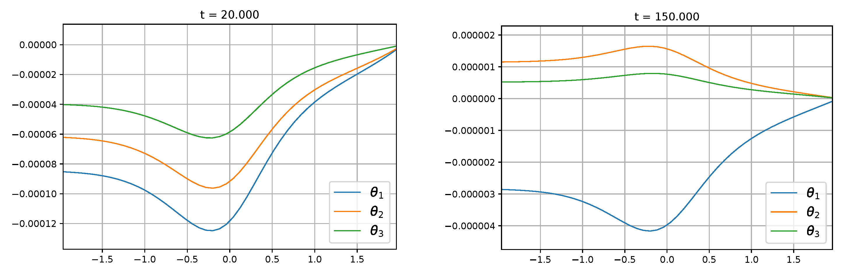
4.2. Well-Balanced Test

In order to show the well-balance properties of the numerical scheme, we perform a numerical simulation of a lake-at-rest steady test. We set the following bathymetry function,

$$b\left(x\right)=\frac{1}{2}{e}^{-x^2},$$

and a constant free surface $\eta =2$. In this problem, the relative density is set to 1, and the initial velocity is zero. Figure 7 (left) depicts the free surface and bathymetry at $t=150$ s, unchanged with respect to the initial condition. Figure 7 (right) shows a zoom on the surface and we can see that the model is exact up to machine precision, even for long time simulations.

A more interesting situation corresponds to the stratified solution described by (14). Let us consider here a particular solution of this family with three layers ($1\le \alpha \le 3$):

$$\begin{array}{c}{u}_{\alpha }=0,\eta \left(x\right)=1,z_b\left(x\right)=\frac{1}{2}{e}^{-x^2},h\left(x\right)=1-z_b\left(x\right),\\ \begin{array}{cc}{\theta }_1\left(x\right)\hfill & =h{\left(x\right)}^4{K}_3+3h{\left(x\right)}^2{K}_2+K_1,\hfill \\ {\theta }_2\left(x\right)\hfill & =h{\left(x\right)}^2{K}_2+K_1,\hfill \\ {\theta }_3\left(x\right)\hfill & =K_1.\hfill \end{array}\end{array}$$

(42)

The constant values $K_i$ are chosen in order to have a stable stratified profile in the vertical direction, that is, ${\theta }_3\left(x\right)\le {\theta }_2\left(x\right)\le {\theta }_1\left(x\right)$. Here, we consider $K_1=1.01$, $K_2=0.02$ and $K_3=0$. Note that, if a stratification expression like (13) is used, then the coefficients $K_i$ tends to zero with the increasing of the number of layers.

The numerical scheme described in Section 3 cannot preserve the steady state (42). Figure 8 shows the free surface and velocities at $t=10$ s when (42) is given as initial condition on the domain $[-5,5]$, discretized with 200 cells.

Nevertheless, it is possible to modify scheme (35) or (33) in order to improve their well-balanced properties and, in particular, to preserve this stationary solution. Following [48], it is possible to modify the reconstruction procedure in such a way that these particular solutions are preserved. Remark that here we are focusing on preserving just this particular solution. The procedure is briefly described in what follows. Future and ongoing works will aim at generalizing the technique so that the numerical scheme is able to preserve a larger family of steady states.

Let us modify (35) in order to improve its well-balanced property and, in particular, to preserve the stationary solution (42). We denote by ${\mathit{w}}_e\left(x\right)$ this particular stationary solution. According to [48], the first stage is to define a reconstruction operator that preserves ${\mathit{w}}_e\left(x\right)$. The idea is quite simple: first define the fluctuation with respect to ${\mathit{w}}_e\left(x\right)$ that is at each cell and at each time step we compute the quantities,

$${\mathit{w}}_{f,i}^n\left(t\right)={\mathit{w}}_i^n-{\mathit{w}}_e\left(x_i\right),$$

where $x_i$ is the center of the cell $I_i$. Note that ${\mathit{w}}_e\left(x_i\right)$ is the evaluation of the stationary solution at the center of the cell that is a second order approximation of its cell average on the cell $I_i$. Next, we apply the standard second order reconstruction previously described to the fluctuations ${\mathit{w}}_{f,i}^n$. Let us denote these reconstructions by ${\mathit{R}}_i^f\left(x\right)$. Finally, the reconstruction for $\mathit{w}$ is defined as follows:

$${\mathit{R}}_i\left(x\right)={\mathit{w}}_e\left(x\right)+{\mathit{R}}_i^f\left(x\right).$$

Special care should be taken for the quadrature formula applied for the integral appearing in (35). Again, we follow [48] in order to propose a quadrature formula that preserves the well-balanced character of the reconstruction and, therefore, of the numerical scheme.

Now, if we apply (35) with the previous reconstruction procedure, the numerical scheme also preserves the stationary solution (42). Figure 9 shows the errors for the relative density and velocities at time $t=150s$ when compared to the exact steady state and those are of the order of the machine precision.

Now, let us consider a small perturbation on the stationary solution (42), where now we consider

$$\eta (x,0)=1+\frac{1}{10}{e}^{-10x^2},$$

as the initial free surface. The relative densities ${\theta }_{\alpha }$ and velocities $u_{\alpha }$ remain the same. The initial free surface and relative densities are shown in Figure 10. We consider the same domain as previously, discretized with the same number of cells. The relative densities and the free surface are fixed as the right boundary condition, while open boundary conditions are considered on the left. Figure 11 and Figure 12 show the difference of the relative density with respect to the one given by the steady state. As it can be seen, the relative density slowly converges to the stationary solution up to machine precision (see Figure 12).

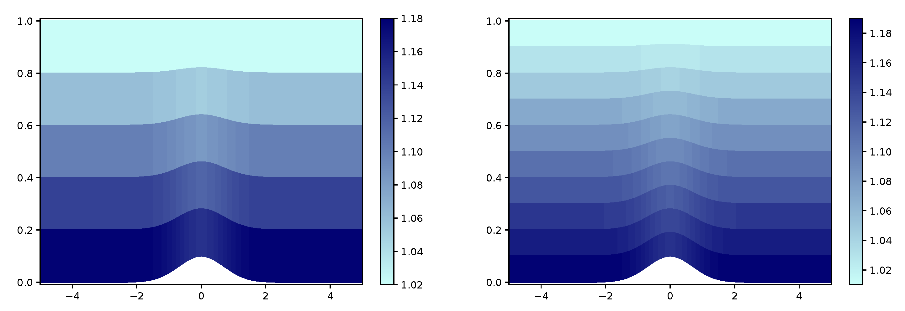
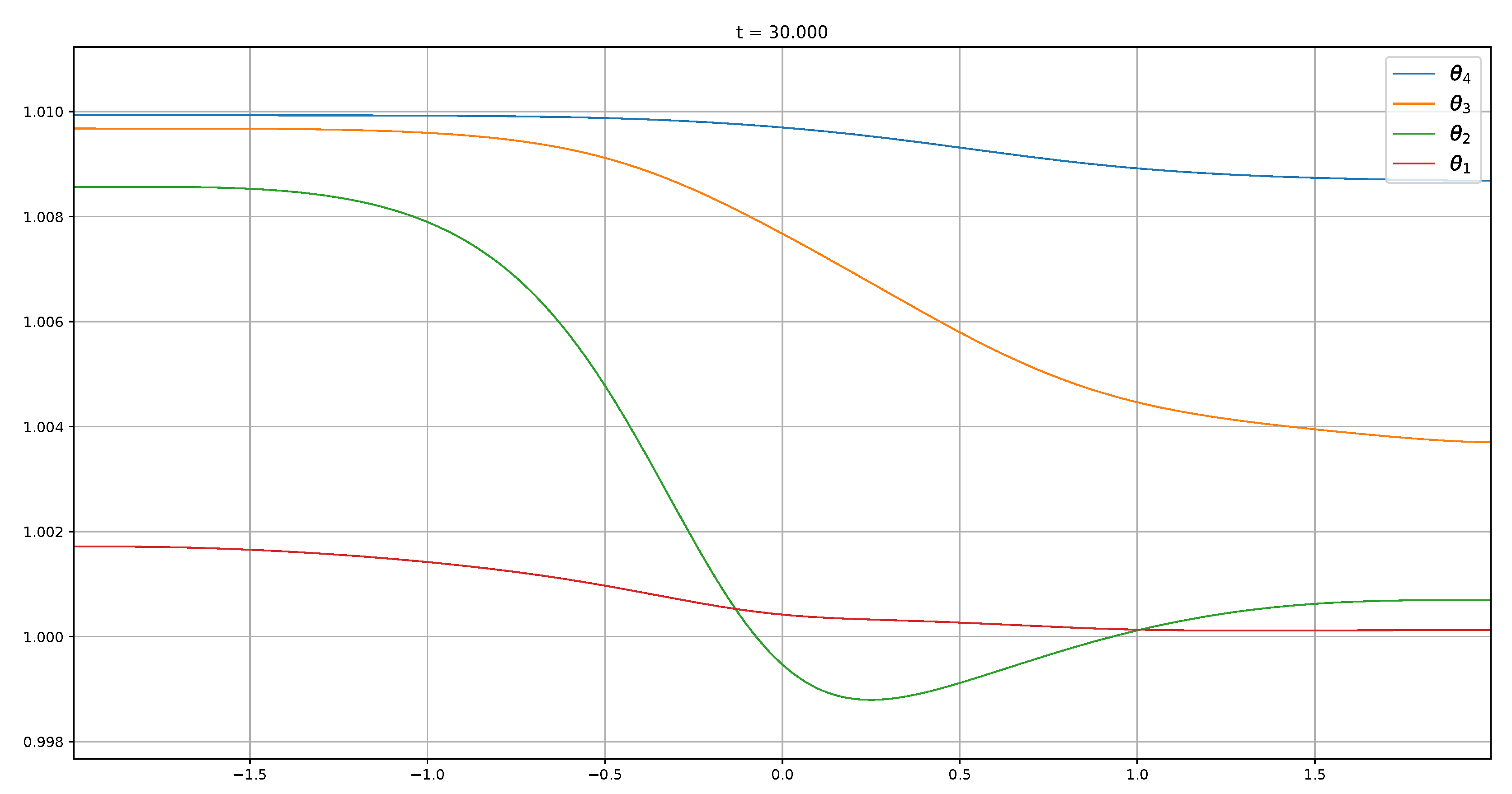
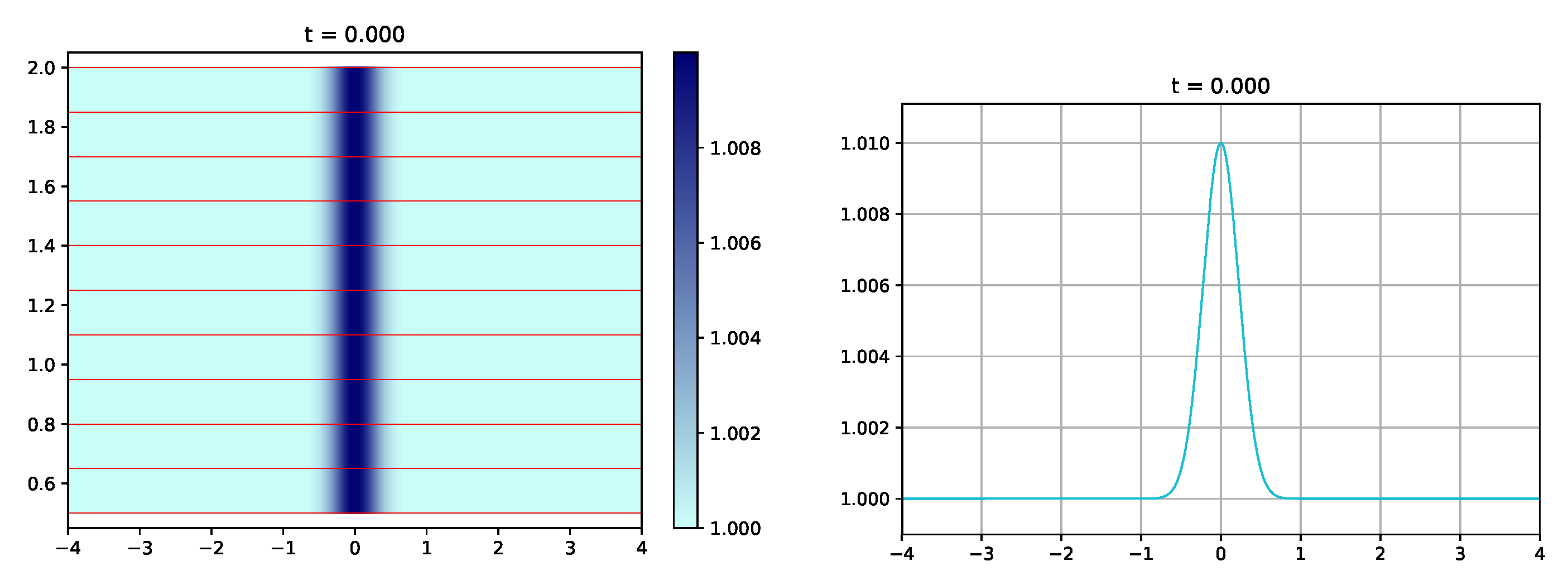
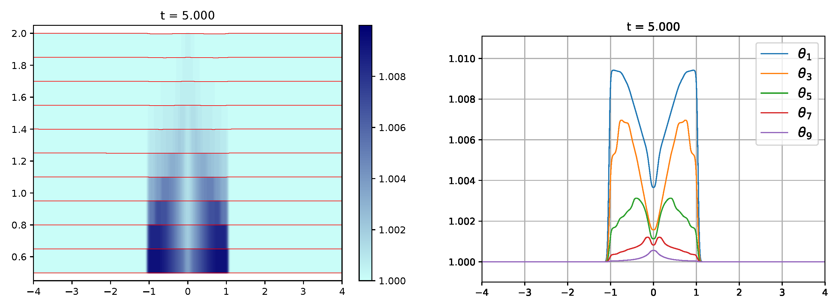
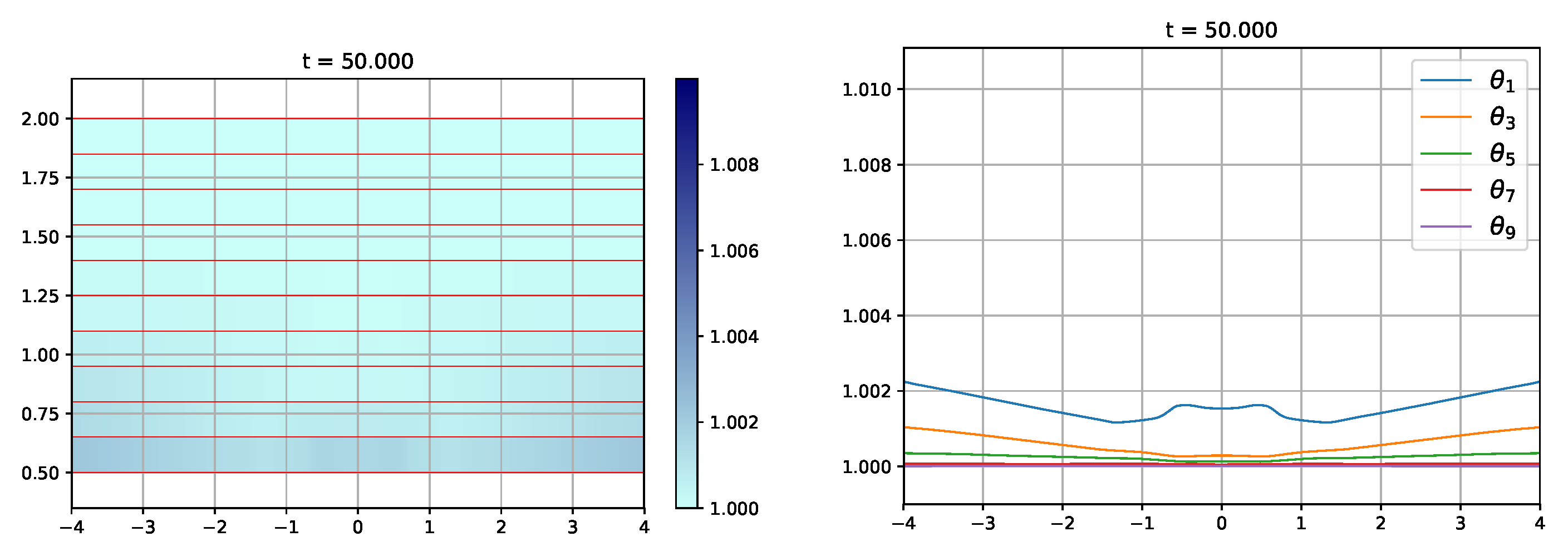
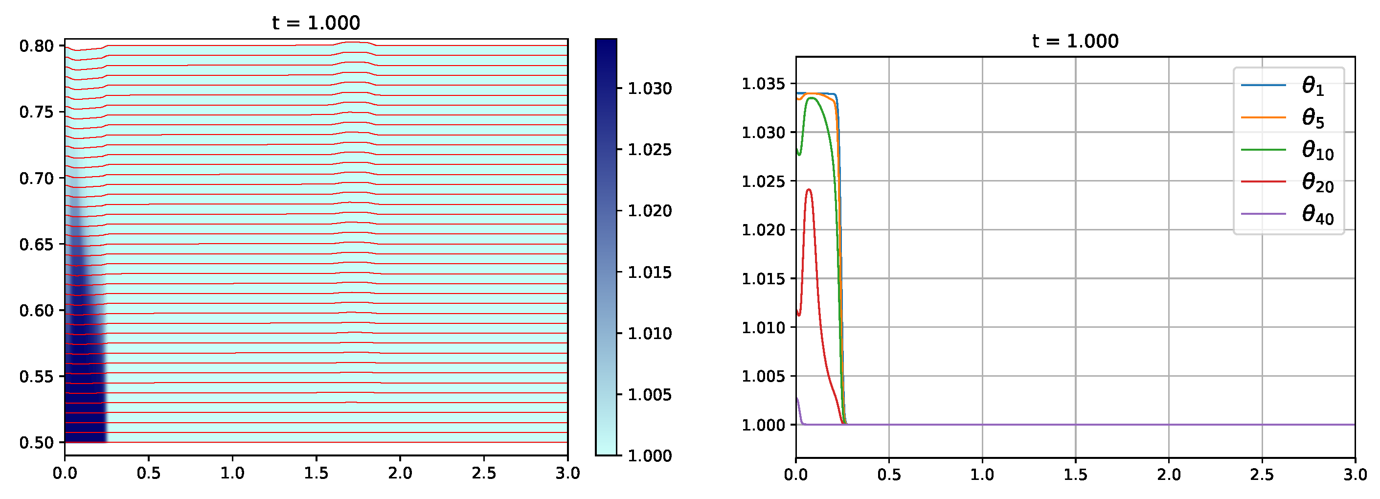
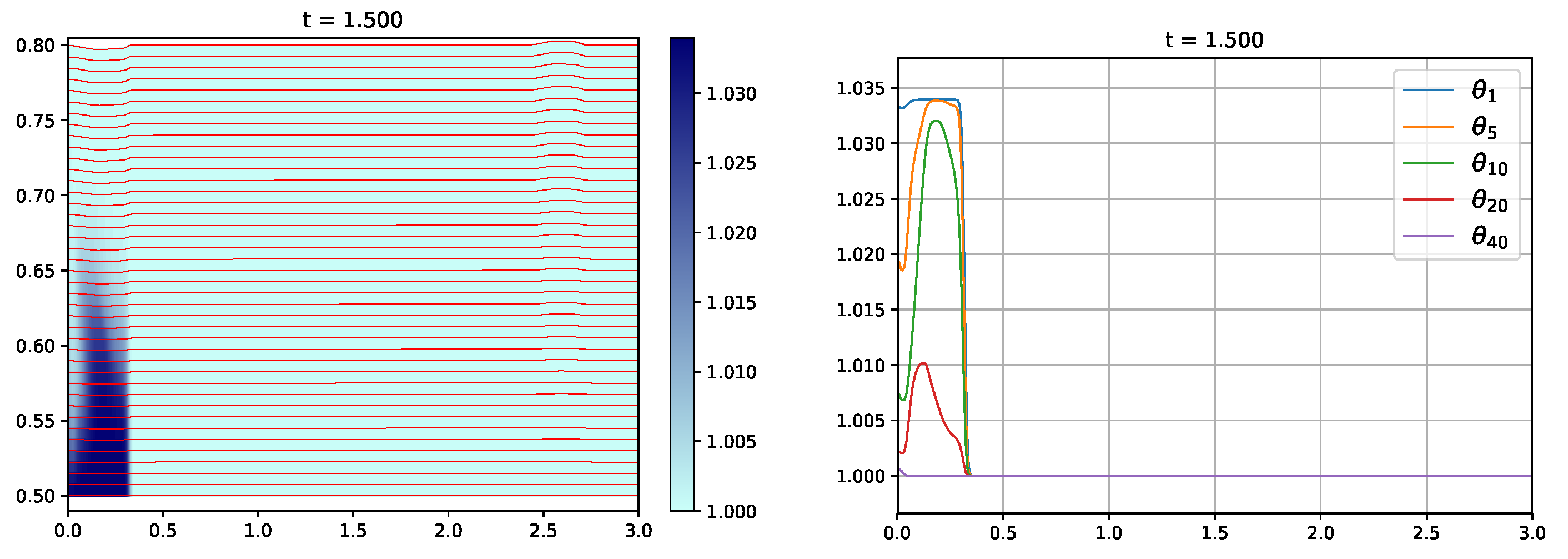
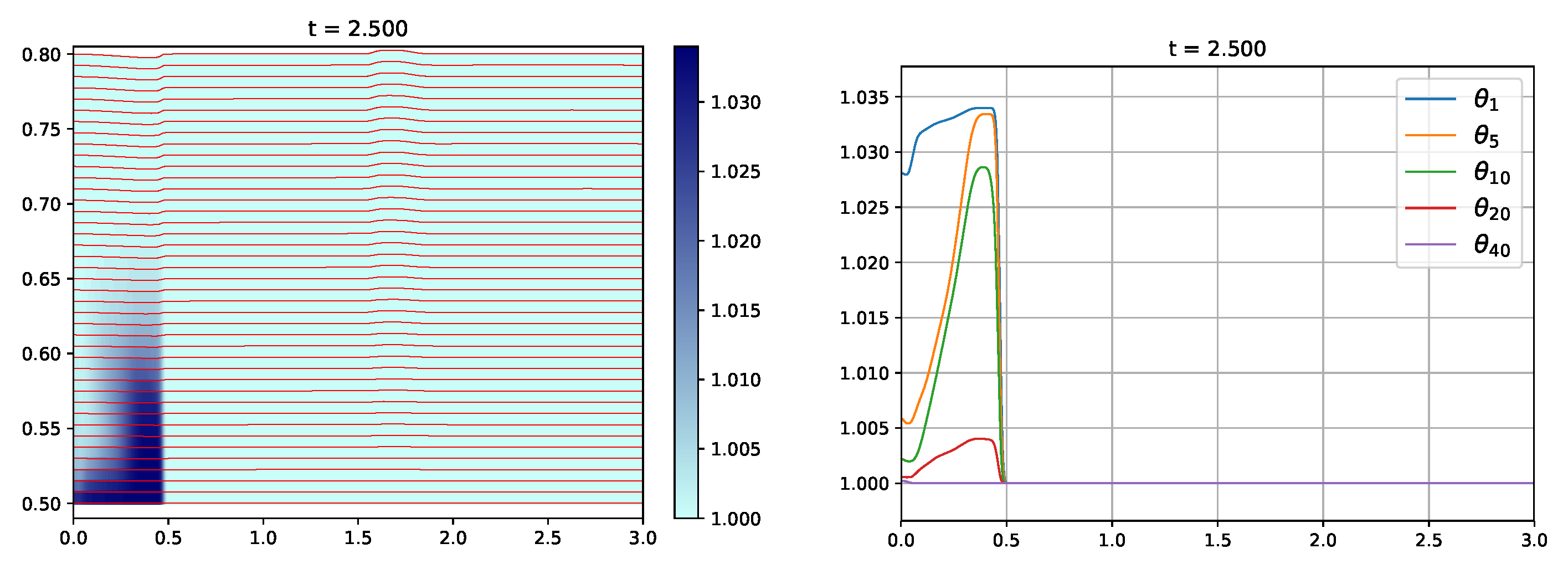
4.3. Simulation for a Smooth Distribution of Relative Density

We perform now a simulation with a smooth profile for the relative density $\theta$. We fix the domain $[-4,4],$ discretized with 800 volume cells and we choose $M=10$ layers. The relative density $\theta$ is initially equal in all the layers and given by

$${\theta }_{\alpha }(t=0,x)=1+\frac{1}{100}{e}^{-10x^2},$$

while the bathymetry and the free surface are constant and equal to $0.5$ and $1.5$, respectively. We consider open boundary conditions. The initial condition is shown in Figure 13. Figure 14, Figure 15, Figure 16 and Figure 17 show the evolution of the relative density for different times. We see that the relative density tends to go downwards and towards the sides, but, at different velocities, due to the difference of pressure between layers, forming a shock (see Figure 16). Eventually, for large times, the solution becomes stratified in layers (see Figure 17). A dual representation has been chosen for the relative density. On the right-hand side of the figure, we show the graph of the relative density for a choice of some layers, so that they are representative of the evolution of the problem. On the left-hand side, we show the relative density within the layers through a heat map.

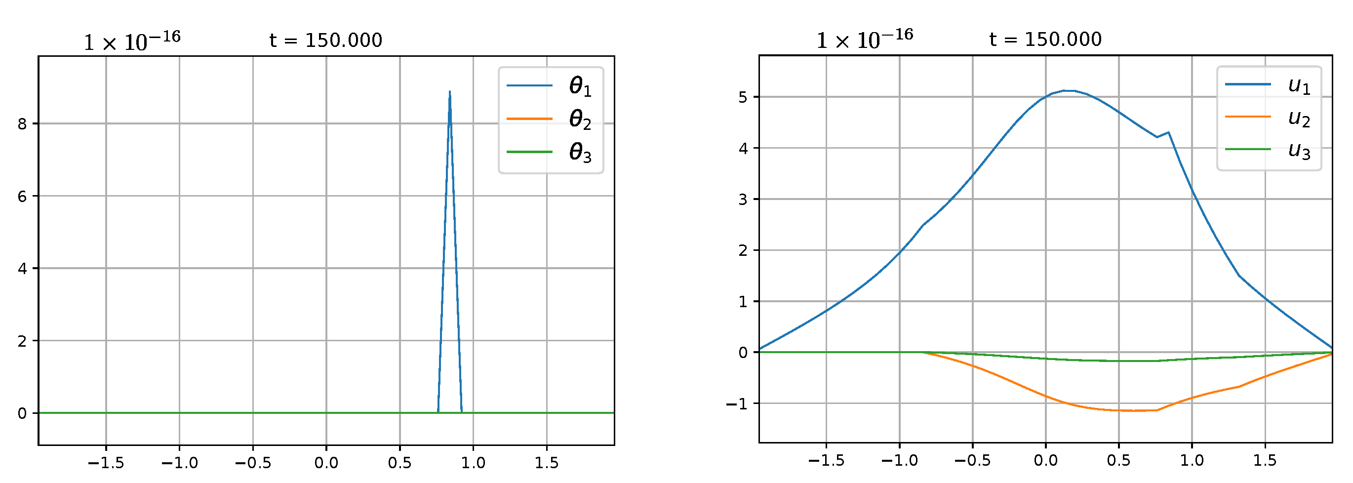
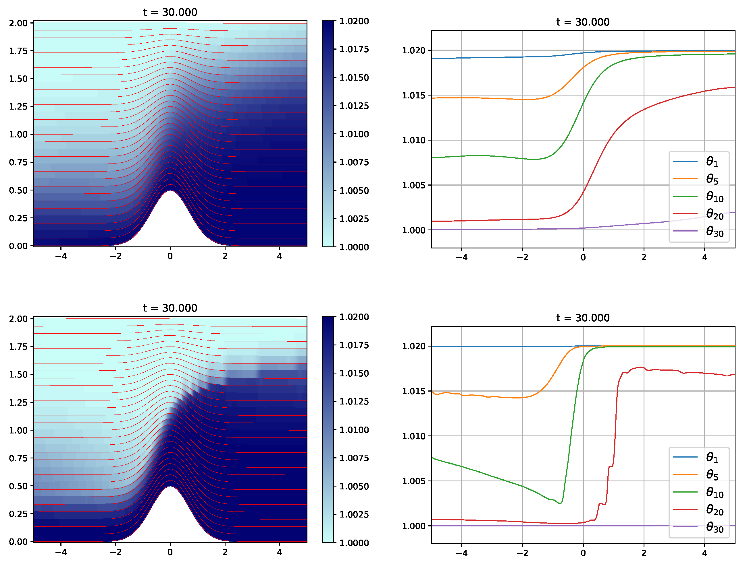
4.4. Simulation of a Lock-Exchange in a Flat Channel

We propose now to perform the test corresponding to the experimental data presented in [35]. There, the authors propose a laboratory experiment in a 3 m long channel, where a gatebox of length $0.1$ m is placed within the channel containing a fluid with density ${\rho }_1.$ The rest of the channel contains a fluid of density ${\rho }_0,$ with ${\rho }_1>{\rho }_0$ The gate box is opened and its fluid is released into the flume. The density ${\rho }_0$ is 1000 kg/m${}^3$ while ${\rho }_1$ is 1034 kg/m${}^3$. Thus, we consider

$$\theta \left(x\right)=\left\{\begin{array}{c}1.034\mathrm{if}x\le 0.1,\hfill \\ 1.0\mathrm{if}x>0.1.\hfill \end{array}\right.$$

(43)

The initial height of the water is constant and equal to $0.3$ m while the bathymetry is the constant function $b=0.5$. This initial condition is shown in Figure 18. We consider the domain in $[0,3]$ discretized with 800 volume cells. We impose reflecting no-slip boundary conditions.

For the particular case of $M=40$ layers, we show in Figure 19, Figure 20, Figure 21, Figure 22, Figure 23, Figure 24 and Figure 25 the evolution of the density distribution at different times. We observe how a shock is formed once the fluid in the gate box is released. The propagation of this shock corresponds to the front position described earlier. The relative density profile at the left boundary of the channel is not an effect of the numerical treatment of the reflecting no-slip boundary conditions. A similar effect can be also observed in the laboratory experiment performed in [35].

In [35], the authors obtain the position of the head of the gravity current with respect to time. In Figure 26 and Figure 27, we can see the comparison for the front position between the experimental data and the results obtained with the numerical approach presented here. The numerical simulations have been obtained using $M=15,20,30$, and 40 layers. We see that the larger the number of layers, the better agreement we have between experimental and numerical data. Even for $M=20$, the results are quite good, despite the fact that non-hydrostatic effects, usually present in such situations (see [49]), are not taken into account.

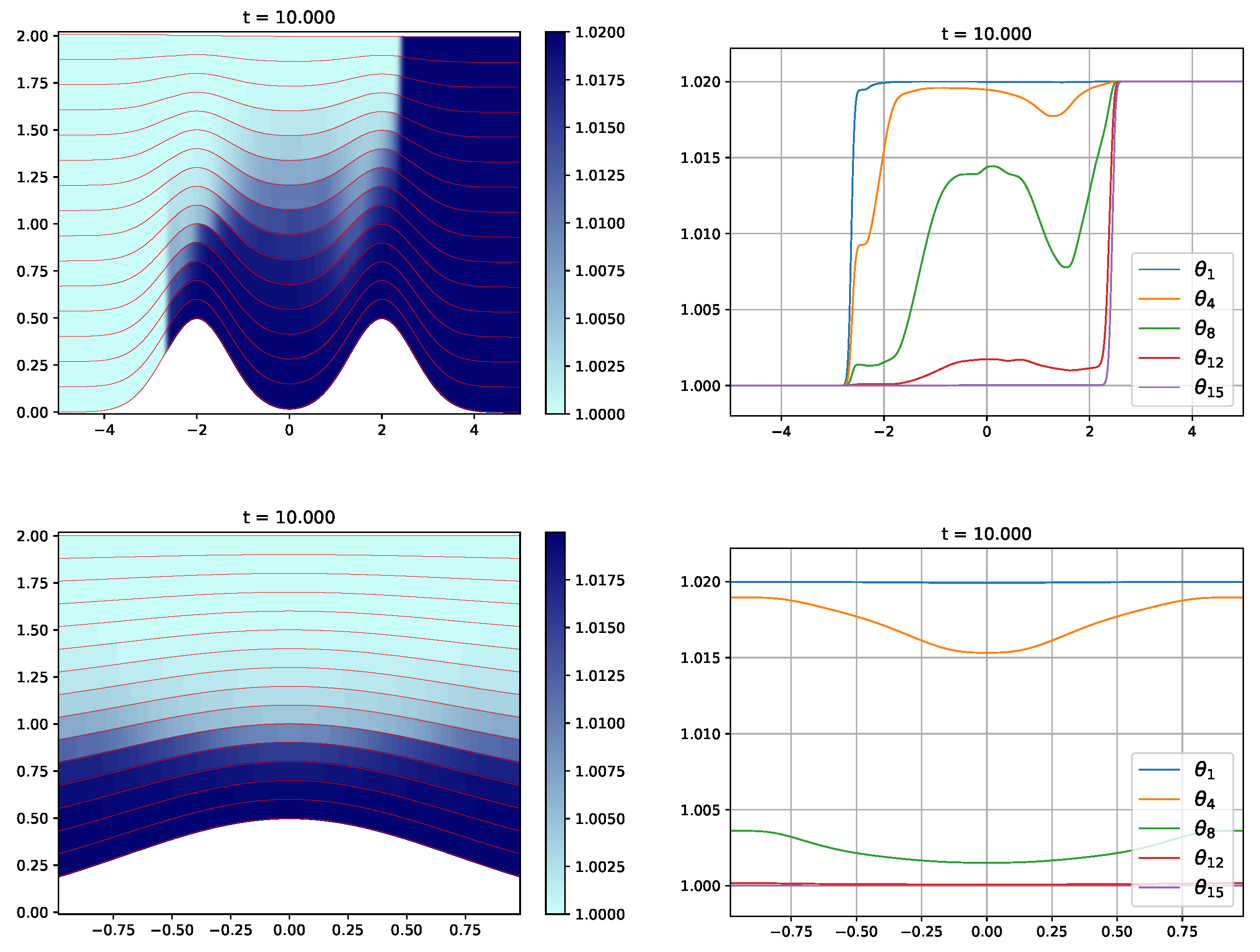
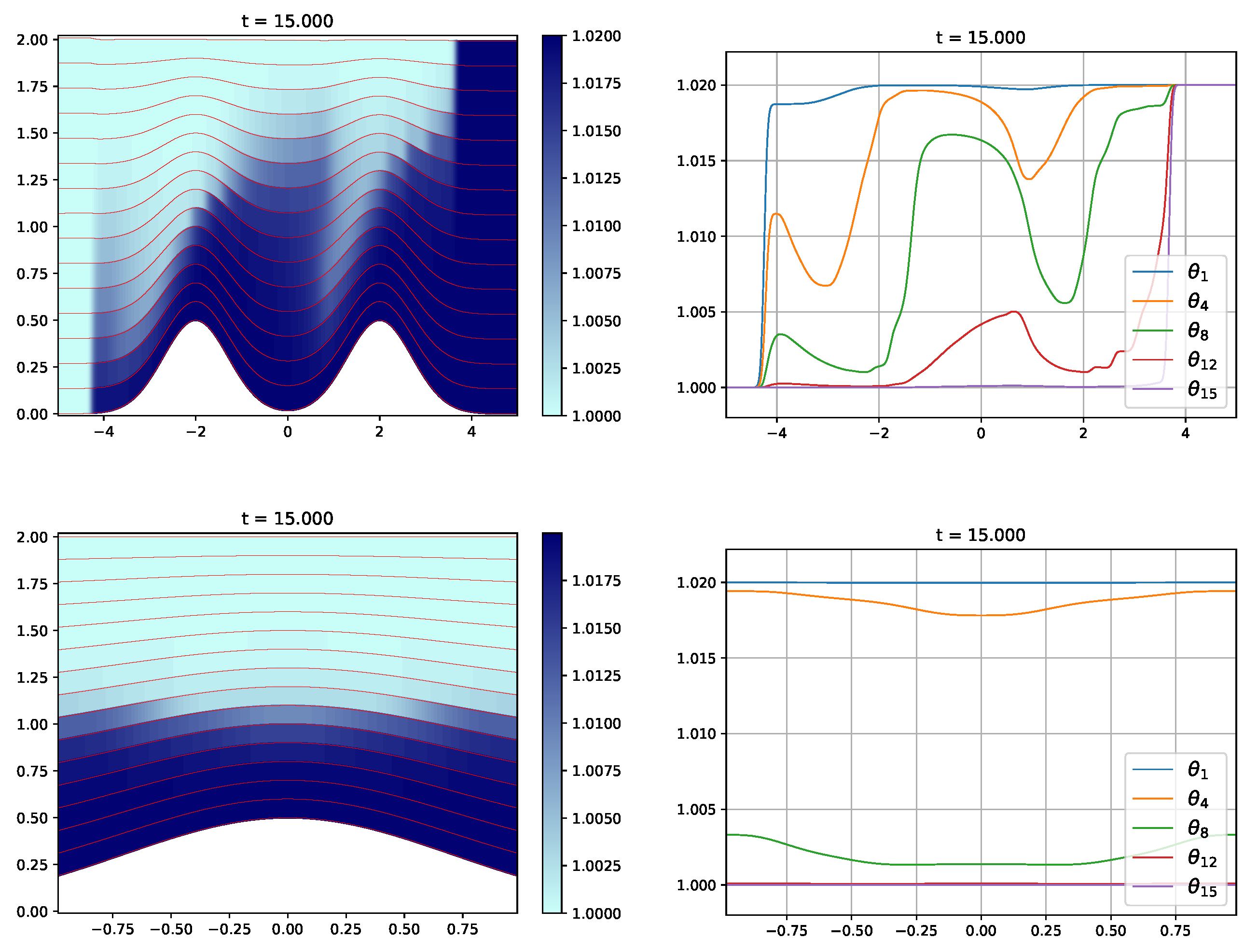
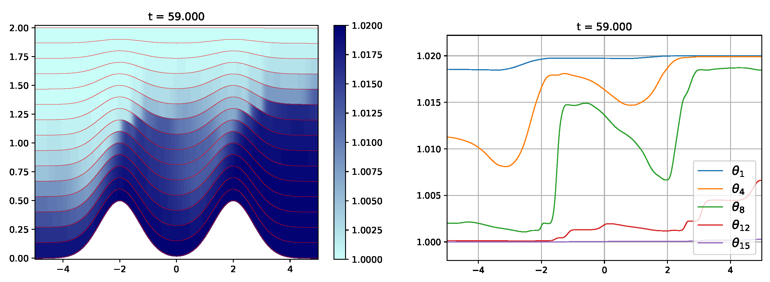
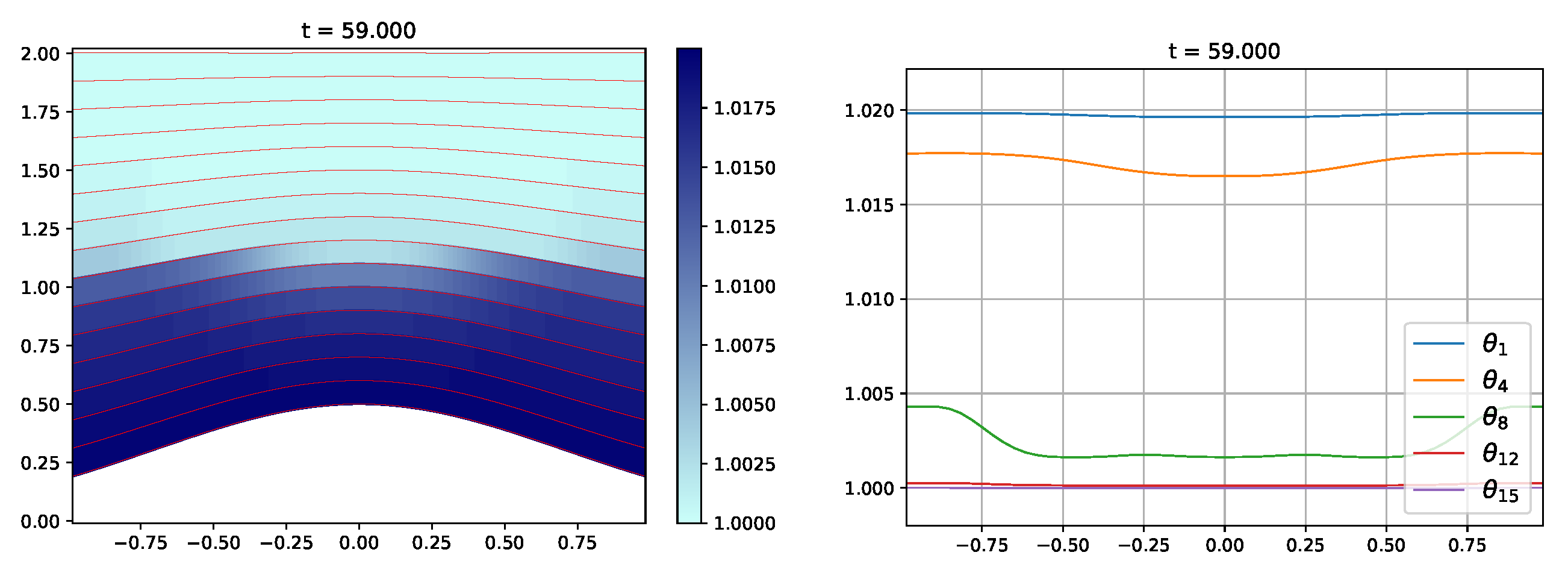
4.5. Simulation of a Dam Break Problem with a Non Constant Bathymetry Function

We consider the domain $[-5,5]$ and a bathymetry function given by

$$z_B\left(x\right)=\frac{1}{2}{e}^{-x^2},$$

(44)

and a constant free surface $\eta =2$ m. A dam break problem in the relative density is considered as an initial condition by setting

$$\theta \left(x\right)=\left\{\begin{array}{c}1.0\mathrm{if}x\le 0,\hfill \\ 1.02\mathrm{if}x>0.\hfill \end{array}\right.$$

(45)

We fix $M=30$ as the number of layers and discretize the domain with 1000 volume cells. Free-flow open boundary conditions are considered. The initial condition is shown in Figure 28 while the evolution of the fluid is depicted in Figure 29, Figure 30, Figure 31, Figure 32 and Figure 33 for different times. In this test, we also compare the first and second order schemes. In particular, we observe a sharp transition of density over the obstacle, especially in the second order case. This kind of profile is common in gravity currents over obstacles (see [50]).

4.6. Simulation of a Dam Break Problem in Two Dimensions

As we have said, although the models and numerical scheme are introduced for the 1D case for the sake of simplicity, everything can be easily extended to the 2D case. To illustrate this fact, we show here a 2D simulation. We fix the domain $(x,y)\in [-5,5]\times [-1,1]$ where non-constant bottom is considered described by

$$z_B(x,y)=\frac{1}{2}{e}^{-({(x+2)}^2+y^2)}+\frac{1}{2}{e}^{-({(x-2)}^2+y^2)}.$$

A constant free surface equal to 2 meters is considered initially. The relative density distribution is set as

$${\theta }_{\alpha }(t=0,x,y)=\left\{\begin{array}{c}1.0\mathrm{if}x\le 0,\hfill \\ 1.02\mathrm{if}x>0.\hfill \end{array}\right.$$

(46)

The domain discretized with 36,000 uniform cells with $\mathsf{\Delta }x=1/60$ and $\mathsf{\Delta }y=1/30$. We impose reflecting no-slip boundary condition at the horizontal walls and free-flow boundary conditions at the vertical ones. We use $M=15$ layers. The initial condition can be seen in Figure 34 and time evolution of the fluid is shown in Figure 35, Figure 36, Figure 37 and Figure 38, where cuts for the $y=0$ and $x=-2$ planes are considered. Figure 39 and Figure 40 also show the upper view of the density distribution for the layer 7. These results are second order accurate.

The numerical simulations performed in this section show that the numerical Section 3 is both robust and accurate, and that the model Section 2 is useful to better understand flows with density fluctuations.

5. Conclusions

We have presented a multilayer shallow water model with variable density. We propose first and second order numerical schemes that preserve the stationary solutions corresponding to water at rest with constant density. Some insight has been briefly given on how to modify the scheme in order to preserve some stratified stationary solutions. The numerical scheme is also positive preserving for the water height. According to the numerical experiments, it seems that it also satisfies the maximum principle for ${\theta }_{\alpha }$. The numerical tests performed are promising, showing robustness and great agreement with laboratory experimental data. The model used and the numerical strategy introduced here will certainly help with a better understanding of density driven currents in geophysical flows.

References

1. De St. Venant, B. Theorie du mouvement non-permanent des eaux avec application aux crues des rivers et a l’introduntion des Marees dans leur lit. Acad. Sci. Comptes Redus 1871, 73, 148–154. [Google Scholar]
2. Cushman-Roisin, B.; Beckers, J.M. Introduction to Geophysical Fluid Dynamics: Physical and Numerical Aspects; Academic Press: Cambridge, MA, USA, 2011. [Google Scholar]
3. Audusse, E.; Bristeau, M.O. Finite-Volume Solvers for a Multilayer Saint–Venant System. Appl. Math. Comput. Sci. 2007, 17, 311–320. [Google Scholar] [CrossRef] [Green Version]
4. Audusse, E.; Bristeau, M.O.; Perthame, B.; Sainte-Marie, J. A multilayer Saint–Venant system with mass exchanges for shallow water flows. Derivation and numerical validation. ESAIM Math. Model. Numer. Anal. 2011, 45, 169–200. [Google Scholar] [CrossRef]
5. Gosse, L. A well-balanced scheme using non-conservative products designed for hyperbolic systems of conservation laws with source terms. Math. Model. Methods Appl. Sci. 2001, 11, 339–365. [Google Scholar] [CrossRef] [Green Version]
6. Macias, J.; Castro, M.J.; González-Vida, J.M.; de la Asunción, M.; Ortega, S. HySEA: An operational GPU-based model for Tsunami Early Warning Systems. In Proceedings of the EGU General Assembly 2014, Vienna, Austria, 27 April–2 May 2014; p. 14217. [Google Scholar]
7. de la Asunción, M.; Castro, M.; Mantas, J.; Ortega, S. Numerical simulation of tsunamis generated by landslides on multiple GPUs. Adv. Eng. Softw. 2016, 99, 59–72. [Google Scholar] [CrossRef]
8. LeVeque, R.J.; George, D.L.; Berger, M.J. Tsunami modelling with adaptively refined finite volume methods. Acta Numer. 2011, 20, 211–289. [Google Scholar] [CrossRef] [Green Version]
9. Barthélemy, E. Nonlinear shallow water theories for coastal waves. Surv. Geophys. 2004, 25, 315–337. [Google Scholar] [CrossRef]
10. Lastra, M.; Mantas, J.M.; Ureña, C.; Castro, M.J.; García-Rodríguez, J.A. Simulation of shallow-water systems using graphics processing units. Math. Comput. Simul. 2009, 80, 598–618. [Google Scholar] [CrossRef]
11. Brufau, P.; Vázquez-Cendón, M.; García-Navarro, P. A numerical model for the flooding and drying of irregular domains. Int. J. Numer. Methods Fluids 2002, 39, 247–275. [Google Scholar] [CrossRef]
12. Gonzalez-Sanchis, M.; Murillo, J.; Latorre, B.; Comin, F.; Garcia-Navarro, P. Transient Two-Dimensional Simulation of Real Flood Events in a Mediterranean Floodplain. J. Hydraul. Eng. ASCE 2012, 138, 629–641. [Google Scholar] [CrossRef] [Green Version]
13. Ersoy, M.; Lakkis, O.; Townsend, P. A Saint–Venant shallow water model for overland flows with precipitation and recharge. arXiv 2017, arXiv:1705.05470. [Google Scholar]
14. Martínez-Cantó, R.; Hidalgo, A. A Methodology Based on Numerical Simulation to Study River Floods. Application to Lower River Omaña Basin. Water Resour. 2019, 46, 844–852. [Google Scholar] [CrossRef]
15. Ersoy, M.; Lakkis, O.; Townsend, P. Numerical simulation of flood inundation using a well-balanced kinetic scheme for the shallow water equations with bulk recharge and discharge. In Proceedings of the EGU General Assembly 2016, Vienna, Austria, 17 April–22 April 2016; Volume 18. [Google Scholar]
16. Dawson, C.; Kubatko, E.J.; Westerink, J.J.; Trahan, C.; Mirabito, C.; Michoski, C.; Panda, N. Discontinuous Galerkin methods for modeling hurricane storm surge. Adv. Water Resour. 2011, 34, 1165–1176. [Google Scholar] [CrossRef] [Green Version]
17. Mandli, K.T.; Dawson, C.N. Adaptive mesh refinement for storm surge. Ocean Model. 2014, 75, 36–50. [Google Scholar] [CrossRef] [Green Version]
18. Tanaka, S.; Bunya, S.; Westerink, J.J.; Dawson, C.; Luettich, R.A. Scalability of an unstructured grid continuous Galerkin based hurricane storm surge model. J. Sci. Comput. 2011, 46, 329–358. [Google Scholar] [CrossRef]
19. Audusse, E.; Bristeau, M.O. A well-balanced positivity preserving “second-order” scheme for shallow water flows on unstructured meshes. J. Comput. Phys. 2005, 206, 311–333. [Google Scholar] [CrossRef]
20. Fernández-Nieto, E.D.; Koné, E.H.; Chacón Rebollo, T. A Multilayer Method for the Hydrostatic Navier–Stokes Equations: A Particular Weak Solution. J. Sci. Comput. 2014, 60, 408–437. [Google Scholar] [CrossRef] [Green Version]
21. Audusse, E.; Bristeau, M.; Decoene, A. Numerical simulations of 3D free surface flows by a multilayer Saint–Venant model. Int. J. Numer. Methods Fluids 2008, 56, 331–350. [Google Scholar] [CrossRef]
22. Bonaventura, L.; Fernández-Nieto, E.D.; Garres-Díaz, J.; Narbona-Reina, G. Multilayer shallow water models with locally variable number of layers and semi-implicit time discretization. J. Comput. Phys. 2018, 364, 209–234. [Google Scholar] [CrossRef] [Green Version]
23. Casulli, V.; Stelling, G.S. Numerical simulation of 3D quasi-hydrostatic, free-surface flows. J. Hydraul. Eng. 1998, 124, 678–686. [Google Scholar] [CrossRef]
24. Casulli, V. A semi-implicit finite difference method for non-hydrostatic, free-surface flows. Int. J. Numer. Methods Fluids 1999, 30, 425–440. [Google Scholar] [CrossRef]
25. Casulli, V.; Zanolli, P. Semi-implicit numerical modeling of nonhydrostatic free-surface flows for environmental problems. Math. Comput. Model. 2002, 36, 1131–1149. [Google Scholar] [CrossRef]
26. Ma, G.; Shi, F.; Kirby, J.T. Shock-capturing non-hydrostatic model for fully dispersive surface wave processes. Ocean Model. 2012, 43, 22–35. [Google Scholar] [CrossRef]
27. Bristeau, M.O.; Mangeney, A.; Sainte-Marie, J.; Seguin, N. An energy-consistent depth-averaged Euler system: Derivation and properties. arXiv 2014, arXiv:1406.6565. [Google Scholar] [CrossRef]
28. Fernández-Nieto, E.D.; Parisot, M.; Penel, Y.; Sainte-Marie, J. A hierarchy of dispersive layer-averaged approximations of Euler equations for free surface flows. Commun. Math. Sci. 2018, 16, 1169–1202. [Google Scholar] [CrossRef] [Green Version]
29. Tumolo, G.; Bonaventura, L. Simulations of Non-hydrostatic Flows by an Efficient and Accurate p-Adaptive DG Method. In Numerical Methods for Flows: FEF 2017 Selected Contributions; Springer International Publishing: Cham, Switzerland, 2020; pp. 41–53. [Google Scholar] [CrossRef]
30. de Luna, T.M.; Fernández Nieto, E.; Castro Díaz, M.J. Derivation of a Multilayer Approach to Model Suspended Sediment Transport: Application to Hyperpycnal and Hypopycnal Plumes. Commun. Comput. Phys. 2017, 22, 1439–1485. [Google Scholar] [CrossRef] [Green Version]
31. Bürger, R.; Fernández-Nieto, E.D.; Andrés Osores, V. A dynamic multilayer shallow water model for polydisperse sedimentation. ESAIM Math. Model. Numer. Anal. 2019. [Google Scholar] [CrossRef] [Green Version]
32. Audusse, E.; Bristeau, M.O.; Pelanti, M.; Sainte-Marie, J. Approximation of the hydrostatic Navier–Stokes system for density stratified flows by a multilayer model: Kinetic interpretation and numerical solution. J. Comput. Phys. 2011, 230, 3453–3478. [Google Scholar] [CrossRef]
33. Bouchut, F.; Zeitlin, V. A robust well-balanced scheme for multi-layer shallow water equations. Discret. Contin. Dyn. Syst. Ser. B 2010, 13, 739–758. [Google Scholar] [CrossRef] [Green Version]
34. Castro, M.; Macías, J.; Parés, C. A Q-scheme for a class of systems of coupled conservation laws with source term. Application to a two-layer 1D shallow water system. ESAIM Math. Model. Numer. Anal. 2001, 35, 107–127. [Google Scholar] [CrossRef] [Green Version]
35. Adduce, C.; Sciortino, G.; Proietti, S. Gravity Currents Produced by Lock Exchanges: Experiments and Simulations with a Two-Layer Shallow-Water Model with Entrainment. J. Hydraul. Eng. 2012, 138, 111–121. [Google Scholar] [CrossRef]
36. Bermúdez, A.; Vázquez, M.E. Upwind methods for hyperbolic conservation laws with source terms. Comput. Fluids 1994, 23, 1049–1071. [Google Scholar] [CrossRef]
37. Creaco, E.; Campisano, A.; Khe, A.; Modica, C.; Russo, G. Head reconstruction method to balance flux and source terms in shallow water equations. J. Eng. Mech. 2010, 136, 517–523. [Google Scholar] [CrossRef]
38. Russo, G.; Khe, A. High order well-balanced schemes based on numerical reconstruction of the equilibrium variables. In Waves and Stability in Continuous Media; World Scientific: Singapore, 2010; pp. 230–241. [Google Scholar]
39. Castro, M.J.; de Luna, T.M.; Parés, C. Well-balanced schemes and path-conservative numerical methods. In Handbook of Numerical Analysis; Elsevier: Amsterdam, The Netherlands, 2017; Volume 18, pp. 131–175. [Google Scholar]
40. Castro, M.J.; Pardo Milanés, A.; Parés, C. Well-balanced numerical schemes based on a generalized hydrostatic reconstruction technique. Math. Model. Methods Appl. Sci. 2007, 17, 2055–2113. [Google Scholar] [CrossRef]
41. Parés, C. Numerical methods for nonconservative hyperbolic systems: A theoretical framework. SIAM J. Numer. Anal. 2006, 44, 300–321. [Google Scholar] [CrossRef]
42. Castro, M.; Fernández-Nieto, E. A Class of Computationally Fast First, Order Finite Volume Solvers: PVM Methods. SIAM J. Sci. Comput. 2012, 34. [Google Scholar] [CrossRef] [Green Version]
43. Audusse, E.; Bouchut, F.; Bristeau, M.O.; Klein, R.; Perthame, B. A Fast and Stable Well-Balanced Scheme with Hydrostatic Reconstruction for Shallow Water Flows. SIAM J. Sci. Comput. 2004, 25, 2050–2065. [Google Scholar] [CrossRef]
44. Morales de Luna, T.; Castro Díaz, M.; Parés, C. Reliability of first order numerical schemes for solving shallow water system over abrupt topography. Appl. Math. Comput. 2013, 219, 9012–9032. [Google Scholar] [CrossRef] [Green Version]
45. Van Leer, B. Towards the ultimate conservative difference scheme. V. A second-order sequel to Godunov’s method. J. Comput. Phys. 1979, 32, 101–136. [Google Scholar] [CrossRef]
46. Zhang, X.; Shu, C.W. On maximum-principle-satisfying high order schemes for scalar conservation laws. J. Comput. Phys. 2010, 229, 3091–3120. [Google Scholar] [CrossRef]
47. Gottlieb, S.; Shu, C.W. Total Variation Diminishing Runge–Kutta Schemes. Math. Comput. 1996, 67. [Google Scholar] [CrossRef] [Green Version]
48. Castro, M.J.; Parés, C. Well-Balanced High-Order Finite Volume Methods for Systems of Balance Laws. J. Sci. Comput. 2020, 82, 48. [Google Scholar] [CrossRef]
49. Escalante, C.; de Luna, T.M.; Castro, M. Non-hydrostatic pressure shallow flows: GPU implementation using finite volume and finite difference scheme. Appl. Math. Comput. 2018, 338, 631–659. [Google Scholar] [CrossRef] [Green Version]
50. Lane-Serff, G.F.; Beal, L.M.; Hadfield, T.D. Gravity current flow over obstacles. J. Fluid Mech. 1995, 292, 39–53. [Google Scholar] [CrossRef]
51. Chandrasekaran, S.; Juckeland, G. OpenACC for Programmers: Concepts and Strategies; Addison-Wesley Professional: Boston, MA, USA, 2017. [Google Scholar]
52. Christgau, S.; Spazier, J.; Schnor, B.; Hammitzsch, M.; Babeyko, A.; Waechter, J. A comparison of CUDA and OpenACC: Accelerating the Tsunami Simulation EasyWave. In Proceedings of the ARCS 2014—2014 Workshop Proceedings on Architecture of Computing Systems, Luebeck, Germany, 25–28 February 2014; pp. 1–5. [Google Scholar]
53. Hoshino, T.; Maruyama, N.; Matsuoka, S.; Takaki, R. CUDA vs OpenACC: Performance Case Studies with Kernel Benchmarks and a Memory-Bound CFD Application. In Proceedings of the 2013 13th IEEE/ACM International Symposium on Cluster, Cloud, and Grid Computing, Delft, The Netherlands, 13–16 May 2013; pp. 136–143. [Google Scholar]
54. Mantas, J.M.; De la Asunción, M.; Castro, M.J. An introduction to GPU computing for numerical simulation. In Numerical Simulation in Physics and Engineering; Springer: Berlin, Germany, 2016; pp. 219–251. [Google Scholar]
Figure 1. Sketch of the multilayer approach.
Mathematics 08 00848 g001
Figure 2. Solution of the ODE (12) for an stratified fluid with M = 5 (left) and M = 10 (right).
Mathematics 08 00848 g002
Figure 3. Solution of the ODE (12) for an stratified fluid with M = 50 (left) and M = 100 (right).
Mathematics 08 00848 g003
Figure 4. Simulation with M = 4 number of layers for a version of the code without an upwind approximation. The relative density θ α is shown.
Mathematics 08 00848 g004
Figure 5. Simulation with M = 4 number of layers for a version of the code with an upwind approximation. The relative density θ α is shown.
Mathematics 08 00848 g005
Figure 6. Free surface (left) and velocities (right) at time t = 0.5 s for the second order scheme.
Mathematics 08 00848 g006
Figure 7. Free surface and bathymetry (left) and zoom of the free surface (right) at time t = 150 s.
Mathematics 08 00848 g007
Figure 8. Free surface (left) and velocities (right) at time t = 10 s: solution obtained with the numerical scheme (35).
Mathematics 08 00848 g008
Figure 9. Difference between the numerical solution at t = 100 s and the exact steady state solution for the relative density θ α (left) and velocities (right).
Mathematics 08 00848 g009
Figure 10. Initial condition for a perturbation of a well-balanced steady state with M = 3 layers. Free surface is on the left and relative densities on the right.
Mathematics 08 00848 g010
Figure 11. Difference on the relative density between the perturbed and unperturbed steady state.
Mathematics 08 00848 g011
Figure 12. Difference on the relative density between the perturbed and unperturbed steady state.
Mathematics 08 00848 g012
Figure 13. Relative density initial condition.
Mathematics 08 00848 g013
Figure 14. Evolution of the relative density at t = 2.5 s.
Mathematics 08 00848 g014
Figure 15. Evolution of the relative density at t = 5 s.
Mathematics 08 00848 g015
Figure 16. Evolution of the relative density at t = 10 s.
Mathematics 08 00848 g016
Figure 17. Evolution of the relative density at t = 50 s.
Mathematics 08 00848 g017
Figure 18. Initial condition.
Mathematics 08 00848 g018
Figure 19. Evolution of the density driven current at t = 0.5 s.
Mathematics 08 00848 g019
Figure 20. Evolution of the density driven current at t = 1 s.
Mathematics 08 00848 g020
Figure 21. Evolution of the density driven current at t = 1.5 s.
Mathematics 08 00848 g021
Figure 22. Evolution of the density driven current at t = 2.5 s.
Mathematics 08 00848 g022
Figure 23. Evolution of the density driven current at t = 5 s.
Mathematics 08 00848 g023
Figure 24. Evolution of the density driven current at t = 10 s.
Mathematics 08 00848 g024
Figure 25. Evolution of the density driven current at t = 20 s.
Mathematics 08 00848 g025
Figure 26. Evolution of the head of the gravity current over time. The left figure depicts the problem with M = 15 number of layers while the right shows the case with M = 20 .
Mathematics 08 00848 g026
Figure 27. Evolution of the head of the gravity current over time. The left figure depicts the problem with M = 30 number of layers while the right shows the case with M = 40 .
Mathematics 08 00848 g027
Figure 28. Initial condition.
Mathematics 08 00848 g028
Figure 29. Distribution of the relative density θ . The first row corresponds to the first order scheme and the second row to the second order scheme.
Mathematics 08 00848 g029
Figure 30. Distribution of the relative density θ . The first row corresponds to the first order scheme and the second row to the second order scheme.
Mathematics 08 00848 g030
Figure 31. Distribution of the relative density θ . The first row corresponds to the first order scheme and the second row to the second order scheme.
Mathematics 08 00848 g031
Figure 32. Distribution of the relative density θ . The first row corresponds to the first order scheme and the second row to the second order scheme.
Mathematics 08 00848 g032
Figure 33. Distribution of the relative density θ . The first row corresponds to the first order scheme and the second row to the second order scheme.
Mathematics 08 00848 g033
Figure 34. Initial condition for a cut in the planes y = 0 (upper row) and x = 2 (lower row).
Mathematics 08 00848 g034
Figure 35. Distribution of θ for a cut in the plane y = 0 (upper row) and x = 2 (lower row).
Mathematics 08 00848 g035
Figure 36. Distribution of θ for a cut in the plane y = 0 (upper row) and x = 2 (lower row).
Mathematics 08 00848 g036
Figure 37. Distribution of θ for a cut in the plane y = 0 (upper row) and x = 2 (lower row).
Mathematics 08 00848 g037
Figure 38. Distribution of θ for a cut in the plane y = 0 (upper row) and x = 2 (lower row).
Mathematics 08 00848 g038aMathematics 08 00848 g038b
Figure 39. Upper view of θ distribution in layer 7.
Mathematics 08 00848 g039
Figure 40. Upper view of θ distribution in layer 7.
Mathematics 08 00848 g040