The Transmuted Odd Fréchet-G Family of Distributions: Theory and Applications

Abstract

The last years, the odd Fréchet-G family has been considered with success in various statistical applications. This notoriety can be explained by its simple and flexible exponential-odd structure quite different to the other existing families, with the use of only one additional parameter. In counter part, some of its statistical properties suffer of a lack of adaptivity in the sense that they really depend on the choice of the baseline distribution. Hence, efforts have been made to relax this subjectivity by investigating extensions or generalizations of the odd transformation at the heart of the construction of this family, with the aim to reach new perspectives of applications as well. This study explores another possibility, based on the transformation of the whole cumulative distribution function of this family (while keeping the odd transformation intact), through the use of the quadratic rank transmutation that has proven itself in other contexts. We thus introduce and study a new family of flexible distributions called the transmuted odd Fréchet-G family. We show how the former odd Fréchet-G family is enriched by the proposed transformation through theoretical and practical results. We emphasize the special distribution based on the standard exponential distribution because of its desirable features for the statistical modeling. In particular, different kinds of monotonic and nonmonotonic shapes for the probability density and hazard rate functions are observed. Then, we show how the new family can be used in practice. We discuss in detail the parametric estimation of a special model, along with a simulation study. Practical data sets are handle with quite favorable results for the new modeling strategy.

1. Introduction

Nowadays, there is still a need for statistical models capable of extracting all the information from the data, in order to communicate on them and make them useful as well. This is particularly the case in engineering, economics, biological studies and environmental sciences. For this reason, several generations of statisticians have concentrated their efforts in improving the desirable properties of the probability distributions at the basis of these models, through various kinds of extensions or generalizations. In this regard, sophisticated mathematical modifications have emerged, with practical use encouraged by the modern informatics developments. A classical strategy consists in adding scale or shape parameter(s), also through the use of special functions (beta, gamma, hypergeometric, etc.), with the aim to make the former distribution more pliant on some important modeling aspects (mean, variance, tails of the distributions, skewness, kurtosis, etc.). Thus, new families of continuous distributions were proposed, including those developed in the following short list of references: [1,2,3,4,5,6,7,8,9,10].

In this study, a hybrid family of continuous distributions is constructed, on the basis of the so-called transmuted-G and odd Fréchet-G families. Alpha motivations behind this family are presented below. First of all, the transmuted-G (T-G) family by [9] is defined by the cumulative distribution function (cdf) and probability density function (pdf) given by

$$\begin{array}{c}\hfill F(x;\lambda ,\zeta )=H(x;\zeta )\left[1+\lambda -\lambda H(x;\zeta )\right],x\in \mathbb{R}\end{array}$$

(1)

and

$$\begin{array}{c}\hfill f(x;\lambda ,\zeta )=h(x;\zeta )\left[1+\lambda -2\lambda H(x;\zeta )\right],x\in \mathbb{R},\end{array}$$

(2)

respectively, where $\left|\lambda \right|\le 1$ (allowing negative value for $\lambda$), $H(x;\zeta )$ and $h(x;\zeta )$ are the cdf and pdf of a baseline continuous distribution, respectively, with $\zeta$ as parameter vector. The definition of $F(x;\lambda ,\zeta )$ is based on the concept of quadratic rank transmutation as described in [9]. As prime remark, one can notice that the cdf of the T-G family can be written as a two component mixture: one is the baseline cdf (obtained for $\lambda =0$) and the other is the exponentiated-G cdf (see [5]) with power parameter two (obtained for $\lambda =1$). Numerous studies proved that the simple polynomial structure behind the T-G family can improve the desirable characteristics of the baseline distribution and make the choice of the baseline distribution less determinant (see [11] (Introduction), and the references therein). In addition, the T-G family positively serves to generalize or extend other existing families. For notable studies in this regard, we refer the reader to the transmuted exponentiated generalized-G by [12], new transmuted-G family by [13], generalized transmuted-G family by [14], transmuted Weibull-G family by [15], transmuted odd Lindley-G family by [16], generalized transmuted-G family by [17], transmuted Gompertz-G family by [18], T transmuted-X family by [19], transmuted transmuted-G family by [20] and transmuted generalized odd generalized exponential-G family by [21], among others.

In parallel of these modern transmuted-G families, [7] proposed the odd Fréchet-G (OFr-G) family, constituting a new and simple family using the Fréchet distribution as main generator. More precisely, it is based on the cdf and pdf given by

$$\begin{array}{c}\hfill Q(x;\theta ,\zeta )=e^{-{\left[\frac{1-G(x;\zeta )}{G(x;\zeta )}\right]}^{\theta }},x\in \mathbb{R}\end{array}$$

(3)

and

$$\begin{array}{c}\hfill q(x;\theta ,\zeta )=\frac{\theta g(x;\zeta ){\left[1-G(x;\zeta )\right]}^{\theta -1}}{G{(x;\zeta )}^{\theta +1}}{e}^{-{\left[\frac{1-G(x;\zeta )}{G(x;\zeta )}\right]}^{\theta }},x\in \mathbb{R},\end{array}$$

(4)

respectively, where $\theta >0$ (a shape parameter), $G(x;\zeta )$ and $g(x;\zeta )$ are the cdf and pdf of a baseline continuous distribution with $\zeta$ as parameter vector, respectively. It is shown in [7] that the OFr-G family is easily applicable for modeling purposes. See also [22] where a special member of the OFr-G family, called the odd Féchet inverse exponential distribution, is applied with success. This was also discussed in several notable extensions and generalizations, as in [23] introducing the extended odd Fréchet family, [24] developing the Fréchet Topp Leone-G family, [25] for the generalized odd inverted-exponential-G family and [26] introducing the extended odd Fréchet-G family. However, all these families are based on thorough transformations of the odd function: $G(x;\zeta )/(1-G(x;\zeta \left)\right)$; none of them investigate a simple and direct modification of $Q(x;\theta ,\zeta )$. As praised in the previous paragraph about the T-G family, a motivated idea is to investigate the tunable quadratic rank transmutation. To the best of our knowledge, this direction of work remains new and promising in view of the respective qualities of the T-G and OFr-G families. We thus introduce the transmuted odd Fréchet-G (TOFr-G) family defined with the cdf and pdf given by Equations (1) and (2) with $H(x;\zeta )$ as Equation (3) and $h(x;\zeta )$ as Equation (4), i.e.,

$$\begin{array}{c}\hfill F(x;\lambda ,\theta ,\zeta )=e^{-{\left[\frac{1-G(x;\zeta )}{G(x;\zeta )}\right]}^{\theta }}\left\{1+\lambda -\lambda e^{-{\left[\frac{1-G(x;\zeta )}{G(x;\zeta )}\right]}^{\theta }}\right\},x\in \mathbb{R}\end{array}$$

(5)

and

$$\begin{array}{c}\hfill f(x;\lambda ,\theta ,\zeta )=\frac{\theta g(x;\zeta ){\left[1-G(x;\zeta )\right]}^{\theta -1}}{G{(x;\zeta )}^{\theta +1}}{e}^{-{\left[\frac{1-G(x;\zeta )}{G(x;\zeta )}\right]}^{\theta }}\left\{1+\lambda -2\lambda e^{-{\left[\frac{1-G(x;\zeta )}{G(x;\zeta )}\right]}^{\theta }}\right\},x\in \mathbb{R},\end{array}$$

(6)

respectively, where the notations of the previous paragraphs have been used. The attractive motivation behind the TOFr-G family is to improve the overall adaptability of the former OFr-G family, through the use of the quadratic rank transmutation, and more specially, the tuning of the additional parameter $\lambda$ (the OFr-G family being obtained with $\lambda =0$). In addition, this modification makes the choice of the baseline distribution less crucial; globally, the joint action of $\lambda$ and $\theta$ in the definition of Equations (5) and (6) ensures a high level of flexibility for important distributional characteristics, such as the mode(s), skewness, kurtosis, mean and variance. We illustrate this aspect by discussing in detail a special three-parameter distribution of the family defined with the (standard one-parameter) exponential model as baseline. A graphical analysis reveals that the corresponding probability density and hazard rate functions possess a large panel of monotonic and nonmonotonic shapes, making it desirable for data fitting, among others. Additionally, by considering real data sets of interest, we show that the corresponding model has a better fit behavior in comparison to the transmuted linear exponential distribution developed by [27], new generalized linear exponential proposed by [28], standard Fréchet model and standard exponential model. The gain in terms of statistical modeling is significant.

The rest of the study is structured by the following plan. In Section 2, we complete the presentation of the TOFr-G family by mentioning other important functions of interest, and some special members including the one based on the standard exponential distribution. The mathematical properties of the TOFr-G family are investigated in Section 3, deriving some useful, representation, measures and functions. Turning on the TOFr-G family as potential statistical models, the parametric estimation of the models are discussed via the maximum likelihood method in Section 4, with a simulation study guaranteeing their numerical performance. In Section 5, three practical data sets are analyzed, showing how useful the TOFr-G models can be. Some conclusions are provided in Section 6.

2. Some Complements on the TOFr-G Family

Here, some functions of the TOFr-G family are described, with discussions.

2.1. Other Functions of Interest

We now present some functions of the TOFr-G family having several applications in probability and statistics. First of all, the survival function of the TOFr-G family is given by

$$\begin{array}{c}\hfill S(x;\lambda ,\theta ,\zeta )=1-e^{-{\left[\frac{1-G(x;\zeta )}{G(x;\zeta )}\right]}^{\theta }}\left\{1+\lambda -\lambda e^{-{\left[\frac{1-G(x;\zeta )}{G(x;\zeta )}\right]}^{\theta }}\right\},x\in \mathbb{R}.\end{array}$$

In addition, the cumulative hazard function of the TOFr-G family is given as

$$\begin{array}{c}\hfill R(x;\lambda ,\theta ,\zeta )=-log\left\{1-e^{-{\left[\frac{1-G(x;\zeta )}{G(x;\zeta )}\right]}^{\theta }}\left\{1+\lambda -\lambda e^{-{\left[\frac{1-G(x;\zeta )}{G(x;\zeta )}\right]}^{\theta }}\right\}\right\},x\in \mathbb{R}.\end{array}$$

Finally, the hazard rate function (hrf) of the TOFr-G family is

$$\begin{array}{c}\hfill r(x;\lambda ,\theta ,\zeta )=\frac{\theta g(x;\zeta ){\left[1-G(x;\zeta )\right]}^{\theta -1}{e}^{-{\left[\frac{1-G(x;\zeta )}{G(x;\zeta )}\right]}^{\theta }}\left\{1+\lambda -2\lambda e^{-{\left[\frac{1-G(x;\zeta )}{G(x;\zeta )}\right]}^{\theta }}\right\}}{G{(x;\zeta )}^{\theta +1}\left\{1-e^{-{\left[\frac{1-G(x;\zeta )}{G(x;\zeta )}\right]}^{\theta }}\left\{1+\lambda -\lambda e^{-{\left[\frac{1-G(x;\zeta )}{G(x;\zeta )}\right]}^{\theta }}\right\}\right\}},x\in \mathbb{R}.\end{array}$$

(7)

When the baseline distribution is a lifetime distribution, i.e., with support on $(0,+\infty )$, these functions are particularly meaningful in survival and hazard analyzes. See [29] for instance.

2.2. Notable Members

Here, we introduce three special members of the TOFr-G family. In order to have tractable expressions for Equations (5) and (6), we select the following basic baseline distributions: the exponential, Lindley (see [30,31]) and Lomax (see [32]) distributions. They belong to the family of lifetime distributions. The cdfs and pdfs of these distributions are listed in

Table 1. Some examples of baseline lifetime distributions which can be used to define special members of the transmuted odd Fréchet-G (TOFr-G) family.

Distribution	$\mathit{\zeta }$	$\mathit{G}(\mathit{x};\mathit{\zeta })$	$\mathit{g}(\mathit{x};\mathit{\zeta })$	${\displaystyle \frac{1-\mathit{G}(\mathit{x};\mathit{\zeta })}{\mathit{G}(\mathit{x};\mathit{\zeta })}}$
Exponential	$\left(\beta \right)$	$1-e^{-\beta x}$	$\beta e^{-\beta x}$	${\displaystyle {(e^{\beta x}-1)}^{-1}}$
Lindley	$\left(a\right)$	${\displaystyle 1-\left(1+\frac{ax}{1+a}\right)e^{-ax}}$	${\displaystyle \frac{a^2}{1+a}}$$(1+x)e^{-ax}$	${\displaystyle \frac{1+a+ax}{(1+a)(e^{ax}-1)-ax}}$
Lomax	$(\alpha ,\rho )$	$1-{\left(1+\rho x\right)}^{-\alpha }$	$\alpha \rho {\left(1+\rho x\right)}^{-(\alpha +1)}$	${\displaystyle {\left[{\left(1+\rho x\right)}^{\alpha }-1\right]}^{-1}}$

, as well as the expression of the following central transformation: $[1-G(x;\zeta \left)\right]/G(x;\zeta )$.

The members of the TOFr-G family mentioned in Table 1 are described in detail below. Transmuted odd Fréchet exponential (TOFrE) distribution:

The cdf and pdf of the TOFrE distribution are given by

$$\begin{array}{c}\hfill F(x;\lambda ,\theta ,\beta )=e^{-{(e^{\beta x}-1)}^{-\theta }}\left[1+\lambda -\lambda e^{-{(e^{\beta x}-1)}^{-\theta }}\right],x>0\end{array}$$

and

$$\begin{array}{c}\hfill f(x;\lambda ,\theta ,\beta )=\theta \beta e^{\beta x}{(e^{\beta x}-1)}^{-(\theta +1)}{e}^{-{(e^{\beta x}-1)}^{-\theta }}\left[1+\lambda -2\lambda e^{-{(e^{\beta x}-1)}^{-\theta }}\right],x>0,\end{array}$$

respectively, where $\left|\lambda \right|\le 1$ and $\beta ,\theta >0$. The corresponding hrf can be expressed as

$$\begin{array}{c}\hfill h(x;\lambda ,\theta ,\beta )=\theta \beta e^{\beta x}{(e^{\beta x}-1)}^{-(\theta +1)}{e}^{-{(e^{\beta x}-1)}^{-\theta }}\frac{1+\lambda -2\lambda e^{-{(e^{\beta x}-1)}^{-\theta }}}{1-e^{-{(e^{\beta x}-1)}^{-\theta }}\left[1+\lambda -\lambda e^{-{(e^{\beta x}-1)}^{-\theta }}\right]},x>0.\end{array}$$

Transmuted odd Fréchet Lindley (TOFrLi) Distribution:The cdf and pdf of the TOFrLi distribution are given by

$$\begin{array}{c}\hfill F(x;\lambda ,\theta ,a)=e^{-{\left[\frac{1+a+ax}{(1+a)(e^{ax}-1)-ax}\right]}^{\theta }}\left\{1+\lambda -\lambda e^{-{\left[\frac{1+a+ax}{(1+a)(e^{ax}-1)-ax}\right]}^{\theta }}\right\},x>0\end{array}$$

and

$$\begin{array}{cc}\hfill f(x;\lambda ,\theta ,a)& =\frac{\theta a^2(1+a)(1+x)e^{ax}{\left(1+a+ax\right)}^{\theta -1}}{{\left[(1+a)(e^{ax}-1)-ax\right]}^{\theta +1}}{e}^{-{\left[\frac{1+a+ax}{(1+a)(e^{ax}-1)-ax}\right]}^{\theta }}\hfill \\ \hfill & \times \left\{1+\lambda -2\lambda e^{-{\left[\frac{1+a+ax}{(1+a)(e^{ax}-1)-ax}\right]}^{\theta }}\right\},x>0,\hfill \end{array}$$

respectively, where $\left|\lambda \right|\le 1$ and $\theta ,a>0$. Similarly, the hrf can be expressed by using Equation (7).

Transmuted odd Fréchet Lomax (TOFrLo) distribution:The cdf and pdf of the TOFrLo distribution are given by

$$\begin{array}{c}\hfill F(x;\lambda ,\theta ,\alpha ,\rho )=e^{-{\left[{\left(1+\rho x\right)}^{\alpha }-1\right]}^{-\theta }}\left\{1+\lambda -\lambda e^{-{\left[{\left(1+\rho x\right)}^{\alpha }-1\right]}^{-\theta }}\right\},x>0\end{array}$$

and

$$\begin{array}{cc}\hfill f(x;\lambda ,\theta ,\alpha ,\rho )& =\theta \alpha \rho {\left(1+\rho x\right)}^{\alpha -1}{\left[{\left(1+\rho x\right)}^{\alpha }-1\right]}^{-(\theta +1)}{e}^{-{\left[{\left(1+\rho x\right)}^{\alpha }-1\right]}^{-\theta }}\times \hfill \\ \hfill & \left\{1+\lambda -2\lambda e^{-{\left[{\left(1+\rho x\right)}^{\alpha }-1\right]}^{-\theta }}\right\},x>0,\hfill \end{array}$$

respectively, where $\left|\lambda \right|\le 1$ and $\theta ,\alpha ,\rho >0$. The expression of the hrf follows from Equation (7).

2.3. On the TOFrE Distribution

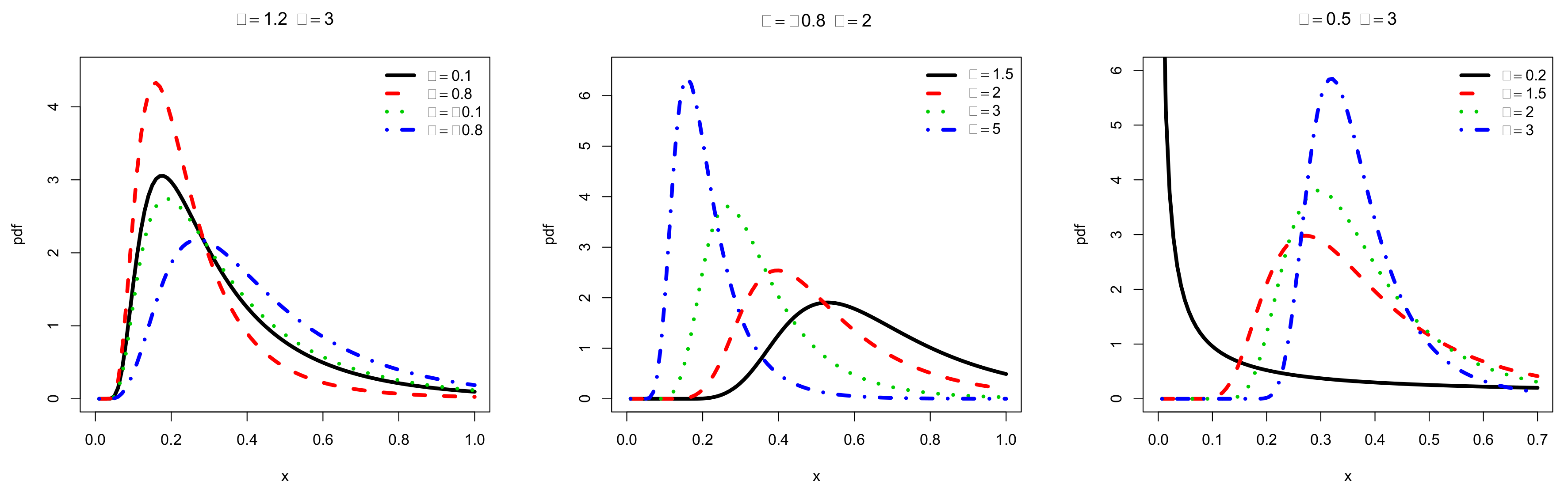
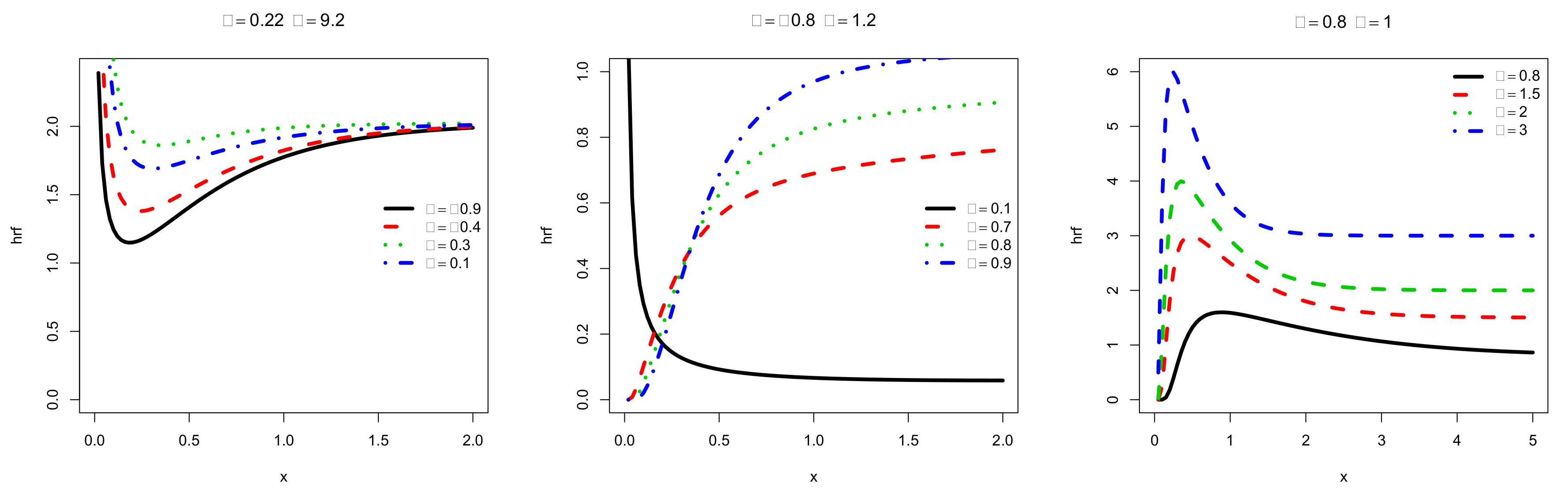
Motivated by an upstream investigation, we chose to put the light on the TOFrE distribution. As a first approach, we display some plots on the corresponding pdf and hrf. By fixing two parameters and varying the one that remains, Figure 1 and Figure 2 show some interesting shapes for the pdf and hrf, respectively.

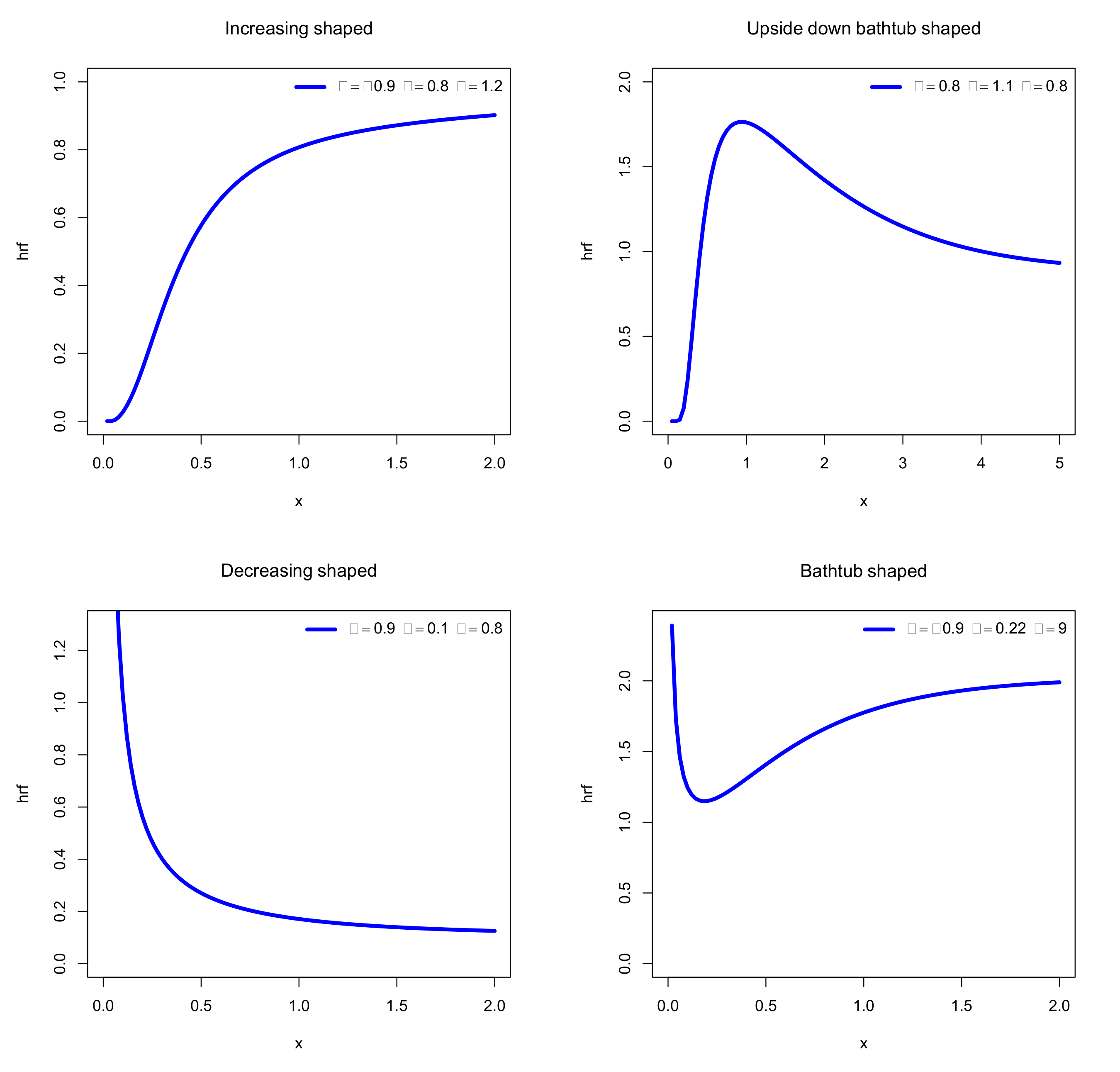
For the considered sets of parameters, we see in Figure 1 that $\lambda$ mainly influences the kurtosis of the distribution. In addition, $\beta$ impacts the central parameters (mean and mode) and kurtosis. For $\theta$, it has a strong effect on the skewness, making the pdf possibly decreasing. Additionally, the following desirable shapes are observed for modeling purposes: almost symmetrical, left or right skewed and reverse J shapes. From Figure 2, we deduce a similar high flexibilities for the hrf, showing bathtub, increasing, decreasing and reversed bathtub shapes, which are welcome for a deep analysis of any lifetime data. Due to their importance, these different shapes are highlighted in Figure 3.

In particular, the hrf of the TOFrE distribution revals to be more pliant than the hrf of the OFrW distribution, special distribution of the former OFr-G family based on the Weibull distribution (see [7] (Subsection 3.1 and Figure 2a)). In this sense, we gain to use the quadratic rank transmutation as described in the TOFr-G family (introducing the parameter $\lambda$), instead of considering the former OFr-G family with an extended baseline distribution (the Weibull distribution extends the exponential distribution, with the add of a shape parameter).

In the next section, thanks to its singular flexibility, an emphasis will be put on TOFrE distribution.

3. Some Results

Here, some mathematical aspects of the TOFr-G family are discussed, and specifically, alternative expressions for the corresponding pdf and cdf, various moments and related functions (incomplete moments, Lorenz curve, etc.).

Henceforth, X denotes a random variable (rv) having the cdf of the TOFr-G family.

3.1. Alternative Expression of the Pdf

Here, we establish a linear/series representation for the pdf of the TOFr-G family in terms of pdfs of the exponentiated-G family. As developed in detail in [33], it allows to provide series expansions of important related measures and functions, such as ordinary moments, moment generating function, incomplete moments and so on. From a practical treatment, we can derive precise approximations of them by replacing the infinite limit by any large integer. This remains an acceptable analytical approach, basically less opaque than using already implemented tools in mathematical softwares. Moreover, as mentioned in [33], the use of such series expansions can be more precise than numerical integration techniques.

Based on Equation (6), $f(x;\lambda ,\theta ,\zeta )$ can be written as

$$\begin{array}{cc}\hfill & f(x;\lambda ,\theta ,\zeta )=\hfill \\ \hfill & \frac{\theta (1+\lambda )g(x;\zeta ){\left[1-G(x;\zeta )\right]}^{\theta -1}}{G{(x;\zeta )}^{\theta +1}}{e}^{-{\left[\frac{1-G(x;\zeta )}{G(x;\zeta )}\right]}^{\theta }}-\frac{2\lambda \theta g(x;\zeta ){\left[1-G(x;\zeta )\right]}^{\theta -1}}{G{(x;\zeta )}^{\theta +1}}{e}^{-2{\left[\frac{1-G(x;\zeta )}{G(x;\zeta )}\right]}^{\theta }}.\hfill \end{array}$$

Now, the power series of the exponential function gives, for $a\in \{1,2\}$,

$$\begin{array}{c}\hfill e^{-a{\left[\frac{1-G(x;\zeta )}{G(x;\zeta )}\right]}^{\theta }}=\sum _{i=0}^{+\infty }\frac{{(-1)}^i{a}^i}{i!}{\left[\frac{1-G(x;\zeta )}{G(x;\zeta )}\right]}^{\theta i}.\end{array}$$

Therefore,

$$\begin{array}{cc}\hfill f(x;\lambda ,\theta ,\zeta )& =\frac{\theta g(x;\zeta ){\left[1-G(x;\zeta )\right]}^{\theta -1}}{G{(x;\zeta )}^{\theta +1}}\sum _{i=0}^{+\infty }\frac{{(-1)}^i}{i!}{\left[\frac{1-G(x;\zeta )}{G(x;\zeta )}\right]}^{\theta i}(1+\lambda -2^{i+1}\lambda )\hfill \\ \hfill & =\theta g(x;\zeta )\sum _{i=0}^{+\infty }\frac{{(-1)}^i}{i!}{\left[1-G(x;\zeta )\right]}^{\theta (i+1)-1}G{(x;\zeta )}^{-\theta (i+1)-1}(1+\lambda -2^{i+1}\lambda ).\hfill \end{array}$$

Now, the generalized binomial formula gives

$$\begin{array}{c}\hfill G{(x;\zeta )}^{-\theta (i+1)-1}=\sum _{j=0}^{+\infty }\left(\genfrac{}{}{0pt}{}{-\theta (i+1)-1}{j}\right){(-1)}^j{\left[1-G(x;\zeta )\right]}^j\end{array}$$

and

$$\begin{array}{c}\hfill {\left[1-G(x;\zeta )\right]}^{\theta (i+1)+j-1}=\sum _{k=0}^{+\infty }\left(\genfrac{}{}{0pt}{}{\theta (i+1)+j-1}{k}\right){(-1)}^{k}G{(x;\zeta )}^k.\end{array}$$

Hence,

$$\begin{array}{c}\hfill f(x;\lambda ,\theta ,\zeta )=\sum _{k=0}^{+\infty }{\varpi }_k{\pi }_{k+1}(x;\zeta ),\end{array}$$

(8)

where ${\pi }_{\upsilon }(x;\zeta )=\upsilon g(x;\zeta )G{(x;\zeta )}^{\upsilon -1}$ denotes the pdf of the exponentiated-G family (with $\upsilon$ as power parameter) and

$${\varpi }_k=\theta \frac{{(-1)}^k}{k+1}\sum _{i,j=0}^{+\infty }\left(\genfrac{}{}{0pt}{}{-\theta (i+1)-1}{j}\right)\left(\genfrac{}{}{0pt}{}{\theta (i+1)+j-1}{k}\right)\frac{{(-1)}^{i+j}}{i!}(1+\lambda -2^{i+1}\lambda ).$$

Similarly, upon integration over $(-\infty ,x)$, the cdf of the TOFr-G family can also be expressed as

$$\begin{array}{c}\hfill F(x;\lambda ,\theta ,\zeta )=\sum _{k=0}^{+\infty }{\varpi }_k{\Pi }_{k+1}(x;\zeta ),\end{array}$$

where ${\Pi }_{\upsilon }(x;\zeta )=G{(x;\zeta )}^{\upsilon }$ denotes the cdf of the exponentiated-G family (with $\upsilon$ as power parameter).

Some applications of the above results will be presented later.

3.2. Quantile Function

Like the cdf, the quantile function characterizes the distribution. It plays an essential role in many statistical applications. The quantile function of the TOFr-G family, say $Q(u;\lambda ,\theta ,\zeta )$, is defined as the inverse function of $F(x;\lambda ,\theta ,\zeta )$. After some algebra, we establish that

$$\begin{array}{c}\hfill Q(u;\lambda ,\theta ,\zeta )=\left\{\begin{array}{cc}{Q}_G\left[{\displaystyle \frac{1}{1+{\left[-log\left(u\right)\right]}^{1/\theta }};\zeta }\right]\hfill & \mathrm{for}\lambda =0,\hfill \\ Q_G\left[\frac{1}{1+{\left\{{\displaystyle -log\left[{\displaystyle \frac{\lambda +1-\sqrt{{(\lambda +1)}^2-4\lambda u}}{2\lambda }}\right]}\right\}}^{1/\theta }};\zeta \right]\hfill & \mathrm{for}\lambda \ne 0,\hfill \end{array}\right.,u\in (0,1),\end{array}$$

where $Q_G(u;\zeta )$ denotes the quantile function corresponding to the baseline distribution.

In the context of the TOFrE distribution, one has $Q_G(u;\zeta )=-(1/\beta )log(1-u)$. Among the possible applications involving $Q(u;\lambda ,\theta ,\zeta )$, we can easily generate values for X; for any realization u of an uniform rv over $(0,1)$, $Q(u;\lambda ,\theta ,\zeta )$ is a realization of X.

In addition, the quantile function allows to define of several shapes measures, as the pioneers Bowley skewness and Moors kurtosis [34,35].

3.3. On the Moments

Here, the moments of the TOFr-G family are discussed, with natural extensions.

Henceforth, $Z_{\upsilon }$ denotes a rv having the cdf and pdf given by ${\Pi }_{\upsilon }(x;\zeta )$ and ${\pi }_{\upsilon }(x;\zeta )$, respectively.

In addition, it is assumed that all the presented sums and integrals exist (in the convergence sense), which is not guarantee a priori since most of them depend on the definition of the baseline distribution.

3.3.1. Ordinary Moments

The ordinary moments of X are the essential ingredients to define important measures of the TOFr-G family, as the mean, variance, coefficients of variations of X, coefficients of skewness and kurtosis, among others. They are determined below. The r-th ordinary moment of the TOFr-G family can be obtained from Equation (8) as

$$\begin{array}{c}\hfill {\mu }_r^{\prime }=E\left(X^r\right)={\int }_{-\infty }^{+\infty }{x}^{r}f(x;\lambda ,\theta ,\zeta )dx=\sum _{k=0}^{+\infty }{\varpi }_{k}E\left(Z_{k+1}^r\right).\end{array}$$

(9)

In full generality, we have $E\left(Z_{\upsilon }^r\right)={\int }_{-\infty }^{+\infty }{x}^r{\pi }_{\upsilon }(x;\zeta )dx$. For instance, in the setting of the TOFrE distribution, the expression of $E\left(Z_{\upsilon }^r\right)$ can be found in [5] (Equation (2.1)), i.e.,

$$\begin{array}{c}\hfill E\left(Z_{\upsilon }^r\right)=\upsilon \frac{r!}{{\beta }^r}\sum _{i=0}^{+\infty }\left(\genfrac{}{}{0pt}{}{\upsilon -1}{i}\right){(-1)}^i\frac{1}{{(i+1)}^{r+1}}.\end{array}$$

From the computational point of view, the following approximation remains acceptable:

$$\begin{array}{c}\hfill E\left(Z_{\upsilon }^r\right)\approx \upsilon \frac{r!}{{\beta }^r}\sum _{i=0}^{40}\left(\genfrac{}{}{0pt}{}{\upsilon -1}{i}\right){(-1)}^i\frac{1}{{(i+1)}^{r+1}},\end{array}$$

(the choice of “40” remains subjective, any large integer can be chosen).

The mean and variance of X are, respectively, given by $\mu ={\mu }_1^{\prime }$ and ${\sigma }^2={\mu }_2^{\prime }-{\mu }^2$. Additionally, the coefficients of skewness and kurtosis are defined by $CS=({\mu }_3^{\prime }-3{\mu }_2^{\prime }\mu +2{\mu }^3)/{\sigma }^3$ and $CK=({\mu }_4^{\prime }-4{\mu }_3^{\prime }\mu +6{\mu }_2^{\prime }{\mu }^2-3{\mu }^4)/{\sigma }^4$.

Table 2. Some values of (${\mu }_r^{\prime }$, $r=1,2,3,4$), along with the variance ${\sigma }^2$, skewness and kurtosis of the TOFrE distribution.

$(\mathit{\lambda },\mathit{\beta },\mathit{\theta })$	${\mathit{\mu }}_1^{\prime }$	${\mathit{\mu }}_2^{\prime }$	${\mathit{\mu }}_3^{\prime }$	${\mathit{\mu }}_4^{\prime }$	${\mathit{\sigma }}^2$	$\mathit{CS}$	$\mathit{CK}$
$(0.2,0.1,2)$	8.5208	87.9640	1143.024	19,136.37	15.3599	2.1884	2.0754
$(0.2,0.5,2)$	1.7041	3.5185	9.1441	30.6181	0.6143	2.1884	78.3214
$(0.2,1,2)$	0.8520	0.8796	1.1430	1.9136	0.1535	2.1884	173.6290
$(0.2,2,2)$	0.4260	0.2199	0.1428	0.1196	0.0383	2.1884	364.2440
$(0.2,0.1,1)$	10.8193	193.5690	5308.916	201,920.7	76.5101	2.3295	4.4139
$(0.2,0.1,3)$	7.8912	68.3049	664.0159	7453.67	6.0334	2.0097	37.3967
$(0.2,0.5,3)$	1.5782	2.7321	5.3121	11.9258	0.2413	2.0097	392.7646
$(0.5,0.5,1)$	1.8889	5.9167	29.5311	212.9278	2.3484	2.6346	17.2340
$(0.9,0.5,1)$	1.5224	3.4820	12.2774	66.0656	1.1641	2.7319	28.9447
$(-0.2,0.5,1)$	2.5303	10.1774	59.7249	469.9344	3.7746	2.0276	10.0319
$(-0.5,0.5,1)$	2.8052	12.0034	72.6651	580.0805	4.1339	1.8796	8.9248
$(-0.9,0.5,1)$	3.1717	14.4381	89.9188	726.9419	4.3780	1.7850	8.5832
$(-0.9,2,2)$	0.5406	0.3445	0.2646	0.2486	0.0522	1.8322	384.4770
$(0.9,2,2)$	0.3531	0.1406	0.0653	0.0374	0.0159	2.2403	1144.3790

presents some of the measures above when X follows the TOFrE distribution. Several sets of parameters values are considered. Strong variations are mainly observed for the mean, variance and kurtosis. In particular, we see that $\beta$ has an important effect on the kurtosis, as already suggested by Figure 1. In line with what has been observed in Figure 1, the skewness remains oriented to the right, but with small variations.

3.3.2. Moment Generating Function

The moment generating function of the TOFr-G family can be obtained from Equation (8) as

$$\begin{array}{c}\hfill M\left(t\right)=E\left(e^{tX}\right)={\int }_{-\infty }^{+\infty }{e}^{tx}f(x;\lambda ,\theta ,\zeta )dx=\sum _{k=0}^{+\infty }{\varpi }_{k}E\left(e^{t{Z}_{k+1}}\right).\end{array}$$

Now, one can notice that $E\left(e^{t{Z}_{\upsilon }}\right)={\int }_{-\infty }^{+\infty }{e}^{tx}{\pi }_{\upsilon }(x;\zeta )dx$. If necessary, we can also express it as $E\left(e^{t{Z}_{\upsilon }}\right)=\upsilon {\int }_0^1{u}^{\upsilon -1}{e}^{t{Q}_G(u;\zeta )}du$.

In the setting of the TOFrE distribution, the expression of $E\left(e^{t{Z}_{\upsilon }}\right)$ can be found in [5] (Equation (2.3)), i.e., for $t\in (0,\beta )$,

$$\begin{array}{c}\hfill E\left(e^{t{Z}_{\upsilon }}\right)=\frac{\Gamma \left(\upsilon +1\right)\Gamma \left({\displaystyle 1-\frac{t}{\beta }}\right)}{\Gamma \left({\displaystyle \upsilon -\frac{t}{\beta }+1}\right)},\end{array}$$

where $\Gamma \left(x\right)={\int }_0^{+\infty }{t}^{x-1}{e}^{-t}dt$, $x>0$, denotes the gamma function.

3.4. Incomplete Moments and Application

Some functions are useful for prediction purposes in lifetime models, finding numerous applications in demography, economics, econometrics, insurance, reliability and medicine. Several of them can be defined through the use of incomplete moments, as discussed below.

3.4.1. Incomplete Moments

Thanks to Equation (8), the $r^{th}$ incomplete moments of X evaluated at $t\ge 0$ can be expressed as

$$\begin{array}{c}\hfill {\vartheta }_r\left(t\right)=E\left(X^r{1}_{\{X\le t\}}\right)={\int }_{-\infty }^t{x}^{r}f(x;\lambda ,\theta ,\zeta )dx=\sum _{k=0}^{+\infty }{\varpi }_{k}E\left(Z_{k+1}^r{1}_{\{Z_{k+1}\le t\}}\right),\end{array}$$

(10)

where, in full generality, $E\left(Z_{\upsilon }^r{1}_{\{Z_{\upsilon }\le t\}}\right)={\int }_{-\infty }^t{x}^r{\pi }_{\upsilon }(x;\zeta )dx$. For instance, in the framework of the TOFrE distribution, we can show that

$$\begin{array}{c}\hfill E\left(Z_{\upsilon }^r{1}_{\{Z_{\upsilon }\le t\}}\right)=\upsilon \frac{1}{{\beta }^r}\sum _{i=0}^{+\infty }\left(\genfrac{}{}{0pt}{}{\upsilon -1}{i}\right){(-1)}^i\frac{\gamma (r+1,t(i+1\left)\beta \right)}{{(i+1)}^{r+1}},\end{array}$$

where $\gamma (x,y)={\int }_0^y{t}^{x-1}{e}^{-t}dt$, $x>0$, $y\ge 0$, denotes the lower incomplete gamma function. Alternatively, we can use the following representation: $E\left(Z_{\upsilon }^r{1}_{\{Z_{\upsilon }\le t\}}\right)=\upsilon {\int }_0^{G(t;\zeta )}{u}^{\upsilon -1}{Q}_G{(u;\zeta )}^{r}du$.

Some functions defined with the incomplete moments are presented below.

3.4.2. Applications

On some residual life functions. The mean residual life and reversed residual life functions have many applications in applied sciences. In addition, as a significant theoretical result, it is proved that the mean residual life function characterizes the distribution (see [36]). See [37], and the references therein.

For the TOFr-G family, we can determine the r-th moment of the residual life. It corresponds to the function of t given as

$$\begin{array}{cc}\hfill {\mu }_r\left(t\right)& =E({(X-t)}^r\mid X>t)=\frac{E\left({(X-t)}^r{1}_{\{X>t\}}\right)}{P(X>t)}\hfill \\ \hfill & =\frac{1}{S(t;\lambda ,\theta ,\zeta )}\sum _{h=0}^r\left(\genfrac{}{}{0pt}{}{r}{h}\right){(-t)}^{r-h}\left[{\mu }_h^{\prime }-{\vartheta }_h\left(t\right)\right],\hfill \end{array}$$

where ${\mu }_h^{\prime }$ and ${\vartheta }_h\left(t\right)$ are given by Equations (9) and (10), respectively.

In particular, the mean residual life function is given as ${\mu }_1\left(t\right)$. In addition, as complementary function, the r-th moment of the reversed residual life is the function of t given by

$$\begin{array}{cc}\hfill m_r\left(t\right)& =E({(t-X)}^r\mid X\le t)=\frac{E\left({(t-X)}^r{1}_{\{X\le t\}}\right)}{P(X\le t)}\hfill \\ \hfill & =\frac{1}{F(t;\lambda ,\theta ,\zeta )}\sum _{h=0}^r\left(\genfrac{}{}{0pt}{}{r}{h}\right)t^{r-h}{(-1)}^h{\vartheta }_h\left(t\right).\hfill \end{array}$$

The mean reversed residual life function is defined by $m_1\left(t\right)$.

Mean deviations. The first incomplete moment allows to define some mean deviations, which find applications in income fields and property in economics (see [34]). In the context of the TOFr-G family, the mean deviation of X about the mean $\mu$ and the mean deviation of X about the median $M=Q(1/2;\lambda ,\theta ,\zeta )$ are defined as

$$\begin{array}{c}\hfill {\delta }_1=E\left(\right|X-\mu \left|\right)=2\mu F\left(\mu \right)-2{\vartheta }_1\left(\mu \right),{\delta }_2=E\left(\right|X-M\left|\right)=\mu -2{\vartheta }_1\left(M\right),\end{array}$$

respectively, where ${\vartheta }_1\left(t\right)$ is the first complete moment given by Equation (10) with $r=1$.

Bonferroni and Lorenz curves. Lorenz and Bonferroni curves are essential tools to determine inequality measures with numerous applications in medicine, reliability and demography. See [38], and the references therein. In the setting of the TOFr-G family, they are defined by

$$\begin{array}{c}\hfill L\left(p\right)=\frac{1}{\mu }{\vartheta }_1\left(q\right),B\left(p\right)=\frac{1}{p\mu }{\vartheta }_1\left(q\right),p\in (0,1),\end{array}$$

respectively, where ${\vartheta }_1\left(t\right)$ is the first complete moment given by Equation (10) with $r=1$ and $q=Q(p;\lambda ,\theta ,\zeta )$.

4. Parametric Estimation

The parametric estimation of the TOFr-G model is now investigated, employing the famous maximum likelihood method.

4.1. Method

The maximum likelihood method provides attractive estimates of the model parameters, called the maximum likelihood estimates (MLEs). They enjoy some asymptotic properties allowing the construction of confidence intervals and some test statistics. In the context of the TOFr-G family, the basics on the MLEs are presented below. Let $(x_1,\dots ,x_n)$ be a random sample of size n from X. Additionally, let $\psi =(\lambda ,\theta ,\zeta )$ be the vector of parameters, with $\zeta =({\zeta }_1,{\zeta }_2\dots )$, the vector of parameters of the baseline model. Then, the log-likelihood function for $\psi$ is given by

$$\begin{array}{cc}\hfill L_n\left(\psi \right)& =\frac{1}{n}\sum _{i=1}^{n}logf(x_i;\lambda ,\theta ,\zeta )=log\left(\theta \right)+\frac{1}{n}\sum _{i=1}^{n}logg(x_i;\zeta )+(\theta -1)\frac{1}{n}\sum _{i=1}^{n}log[1-G(x_i;\zeta )]\hfill \\ \hfill & -(\theta +1)\frac{1}{n}\sum _{i=1}^{n}logG(x_i;\zeta )-\frac{1}{n}\sum _{i=1}^n{\left[\frac{1-G(x_i;\zeta )}{G(x_i;\zeta )}\right]}^{\theta }+\frac{1}{n}\sum _{i=1}^{n}log\left\{1+\lambda -2\lambda e^{-{\left[\frac{1-G(x_i;\zeta )}{G(x_i;\zeta )}\right]}^{\theta }}\right\}.\hfill \end{array}$$

The vector of the MLEs of $\psi =(\lambda ,\theta ,\zeta )$, say $\widehat{\psi }=(\widehat{\lambda },\widehat{\theta },\widehat{\zeta })$, is defined by

$$\widehat{\psi }={argmax}_{\psi }{L}_n\left(\psi \right).$$

The use of any statistical software is possible to provide fine numerical evaluations of them. Now, let ${\psi }_r$ be the $r^{th}$ component of $\psi$ and $J_n\left(\psi \right)={\{-{\partial }^2{L}_n\left(\psi \right)/\partial {\psi }_r\partial {\psi }_s\}}_{r,s}$ be the sample information matrix corresponding to $\psi$ (assuming that $L_n\left(\psi \right)$ is two times differentiable). Then, by denoting ${\widehat{\psi }}_r$ the $r^{th}$ component of $\widehat{\psi }$ and using the asymptotic normality of the MLEs, an asymptotic two-sided confidence interval for ${\psi }_r$ at the level $100(1-\gamma )\%$ with $\gamma \in (0,1)$ is given by $AC{I}_r=\left[L{B}_r,U{B}_r\right]$, where $L{B}_r={\widehat{\psi }}_r-z_{1-\gamma /2}\sqrt{d_r/n}$, $U{B}_r={\widehat{\psi }}_r+z_{1-\gamma /2}\sqrt{d_r/n}$, with $d_r$ is the $r^{th}$ diagonal element of $J_n{\left(\widehat{\psi }\right)}^{-1}$ obtained from $x_1,\dots ,x_n$ and $z_{1-\gamma /2}$ satisfies $Q\left(z_{1-\gamma /2}\right)=1-\gamma /2$, where $Q\left(x\right)$ denotes the quantile function of the normal distribution $\mathcal{N}(0,1)$. The details can be found in the book of [39].

4.2. Numerical Study

This subsection provides a simulation study, offering a numerical check assessing the behavior of the MLEs for the TOFrE model parameters. We determine the mean squared errors (MSEs), as well as average lower bounds (LBs), average upper bounds (UBs) and average lengths (ALs) (i.e., defined by the following generic formula: AL = UB - LB), of the asymptotic two-sided confidence intervals of the model parameters (the levels $90\%$ and $95\%$ are considered). The software Mathematica 9 is used. The following scheme is adopted.

• We generate 1000 random samples $(x_1,\dots ,x_n)$ of size $n=100$, 200, 300 and 500 from the TOFrE distribution.
• We consider the following values for the “supposed true parameters”, with order: $(\theta ,\lambda ,\beta )$: Set1$(1.5,-0.5,2)$, Set2$(1.5,-0.3,1.5)$, Set3$(1.2,-0.5,1)$ and Set4$(1,-0.5,1.5)$.
• We calculate the numerical measures of interest.

Table 3. Numerical measures of interest of the TOFrE model for Set1 (1.5, −0.5, 2).

n	MLEs	MSEs	90%			95%
			LB	UB	AL	LB	UB	AL
100	1.493	0.012	1.275	1.71	0.435	1.233	1.752	0.519
	−0.408	0.075	−1.138	0.321	1.458	−1.277	0.461	1.738
	1.884	0.052	1.449	2.319	0.869	1.366	2.402	1.036
200	1.537	0.01	1.371	1.704	0.333	1.339	1.735	0.397
	−0.431	0.053	−0.951	0.09	1.042	−1.051	0.19	1.241
	1.965	0.032	1.639	2.292	0.653	1.577	2.354	0.778
300	1.457	0.008	1.328	1.585	0.257	1.303	1.61	0.306
	−0.413	0.046	−0.908	0.083	0.99	−1.002	0.177	1.18
	1.967	0.026	1.65	2.285	0.635	1.589	2.345	0.756
500	1.483	0.002	1.37	1.597	0.227	1.348	1.619	0.271
	−0.44	0.042	−0.85	−0.03	0.82	−0.928	0.048	0.977
	1.988	0.018	1.719	2.257	0.539	1.667	2.309	0.642

,

Table 4. Numerical measures of interest of the TOFrE model for Set2 (1.5, −0.3, 1.5).

n	MLEs	MSEs	90%			95%
			LB	UB	AL	LB	UB	AL
100	1.515	0.015	1.27	1.759	0.489	1.223	1.806	0.583
	−0.543	0.106	−1.242	0.157	1.4	−1.376	0.291	1.668
	1.604	0.032	1.228	1.98	0.752	1.156	2.052	0.896
200	1.511	0.011	1.363	1.66	0.297	1.334	1.688	0.354
	−0.214	0.081	−0.883	0.456	1.339	−1.012	0.584	1.596
	1.463	0.025	1.186	1.74	0.555	1.133	1.793	0.661
300	1.482	0.004	1.343	1.622	0.279	1.316	1.648	0.332
	−0.386	0.075	−0.907	0.135	1.042	−1.007	0.235	1.242
	1.544	0.021	1.288	1.799	0.51	1.24	1.847	0.608
500	1.477	0.004	1.378	1.576	0.198	1.359	1.595	0.236
	−0.363	0.066	−0.724	−0.002	0.721	−0.793	0.067	0.86
	1.54	0.019	1.365	1.715	0.35	1.331	1.749	0.417

,

Table 5. Numerical measures of interest of the TOFrE model for Set3 (1.2, −0.5, 1).

n	MLEs	MSEs	90%			95%
			LB	UB	AL	LB	UB	AL
100	1.211	0.014	1.039	1.383	0.344	1.006	1.416	0.41
	−0.475	0.093	−1.083	0.133	1.216	−1.199	0.25	1.449
	0.99	0.013	0.744	1.236	0.493	0.696	1.284	0.587
200	1.196	0.007	1.07	1.322	0.252	1.046	1.346	0.3
	−0.456	0.068	−0.983	0.07	1.053	−1.083	0.171	1.254
	0.992	0.01	0.789	1.196	0.407	0.75	1.235	0.484
300	1.19	0.003	1.082	1.299	0.217	1.061	1.32	0.259
	−0.545	0.062	−0.966	−0.125	0.841	−1.046	−0.045	1.002
	1.009	0.009	0.837	1.18	0.343	0.804	1.213	0.409
500	1.189	0.003	1.097	1.281	0.185	1.079	1.299	0.22
	−0.465	0.044	−0.833	−0.097	0.736	−0.904	−0.027	0.877
	1.001	0.009	0.854	1.149	0.295	0.825	1.177	0.351

and

Table 6. Numerical measures of interest of the TOFrE model for Set4 (1, −0.5, 1.5).

n	MLEs	MSEs	90%			95%
			LB	UB	AL	LB	UB	AL
100	0.983	0.007	0.859	1.106	0.247	0.835	1.13	0.295
	0.01	0.431	−0.602	0.621	1.223	−0.719	0.738	1.457
	1.19	0.12	0.871	1.508	0.637	0.81	1.569	0.759
200	1.002	0.007	0.886	1.118	0.233	0.864	1.141	0.277
	−0.307	0.229	−0.747	0.133	0.88	−0.832	0.217	1.049
	1.424	0.108	1.118	1.73	0.612	1.059	1.788	0.729
300	1.016	0.003	0.926	1.107	0.181	0.908	1.124	0.216
	−0.292	0.138	−0.727	0.144	0.87	−0.81	0.227	1.037
	1.378	0.043	1.114	1.643	0.529	1.063	1.694	0.631
500	0.997	0.003	0.925	1.07	0.145	0.911	1.084	0.173
	−0.365	0.12	−0.713	−0.018	0.695	−0.779	0.049	0.828
	1.457	0.033	1.227	1.688	0.462	1.183	1.732	0.55

list the obtained results.

For the considered sets of parameters, we see that the MLEs stabilize to the true parameters values as the sample size n increases. In addition, the ALs decrease in this case, which is coherent with the well-known theory of the MLEs. This confirms the pertinence of the use of the MLEs in the estimation of the TOFrE model parameters.

5. Applications

In this section, we use the TOFrE model for statistical analyzes of three notorious data sets; the two first data sets are with right exponential-like tails and the third one is with right heavy-like tail. In particular, we aim to compare the fits of the TOFrE model with those of the transmuted linear exponential distribution (TLE) (see [27]), new generalized linear exponential (NGLE) (see [28]), Fréchet (Fr) and exponential (E) models.

The maximum likelihood method is used for all the models, allowing to determine the following measures: AIC, CVM, AD and KS, i.e., Akaike information criterion, Cramer–von Mises, Anderson–Darling and Kolmogorov–Smirnov statistics. In addition, the p-value of the corresponding KS test is provided. The best model is the one with the smallest AIC, CVM, AD and KS values and the biggest p-value for the KS test. The calculations are performed by using the package maxLik proposed by the R software.

5.1. Data Sets I and II (Exponential Tail)

Let us now present our two first data sets of interest, both coming from real-life phenomena.

Data set I. The first data set, called Data set I, is obtained from [40] and comes from a reliability analysis. The data are also available at the following electronic address: https://chesneau.users.lmno.cnrs.fr/DatasetI.txt

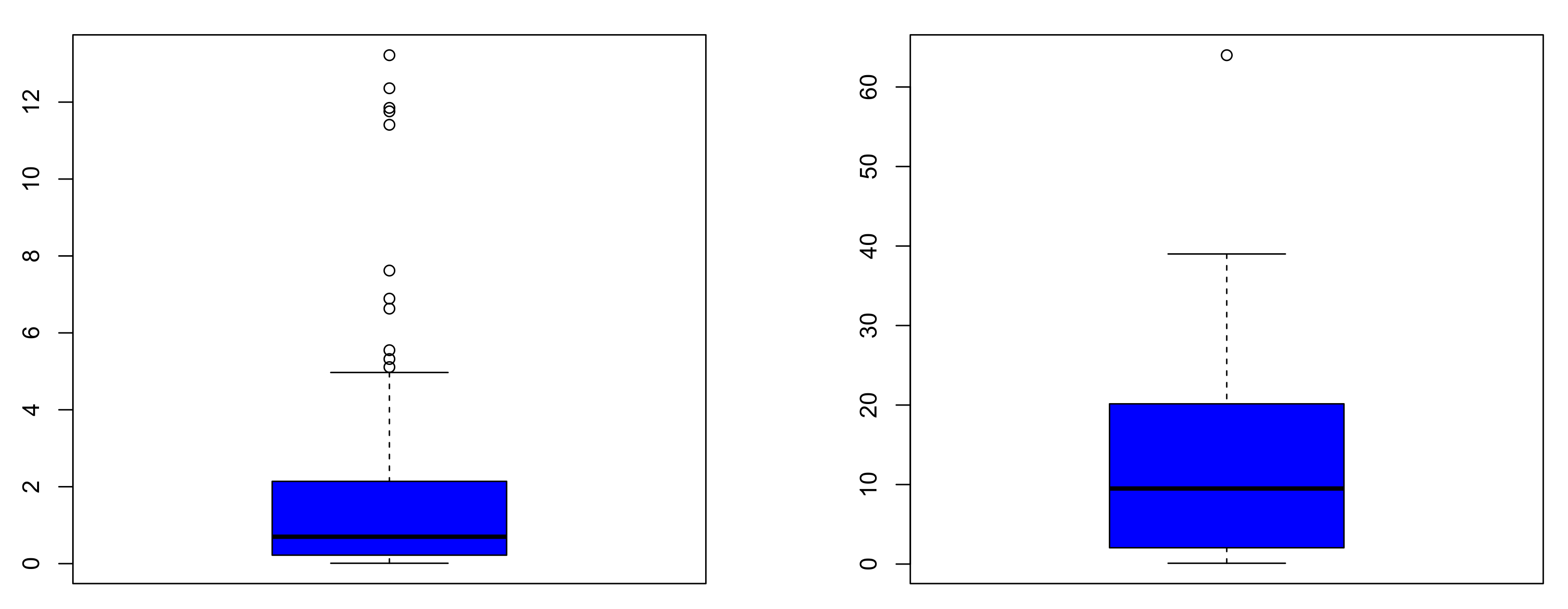
Data set II. The second data set, called Data set II, contains 72 measurements of excedances of the Wheaton river in Canada, between 1958 to 1984. These data were also considered by [41], among others. The data are also available at the following electronic address: https://chesneau.users.lmno.cnrs.fr/DatasetII.txt The basics statistics of these data sets are given in

Table 7. First statistical approaches of Data sets I and II.

Data Set	Number	Mean	Median	Standard Deviation	Skewness	Kurtosis
I	126	1.73	0.7	2.65	2.65	7.22
II	72	12.2	9.5	12.3	1.44	2.73

, with support of the corresponding boxplots in Figure 4.

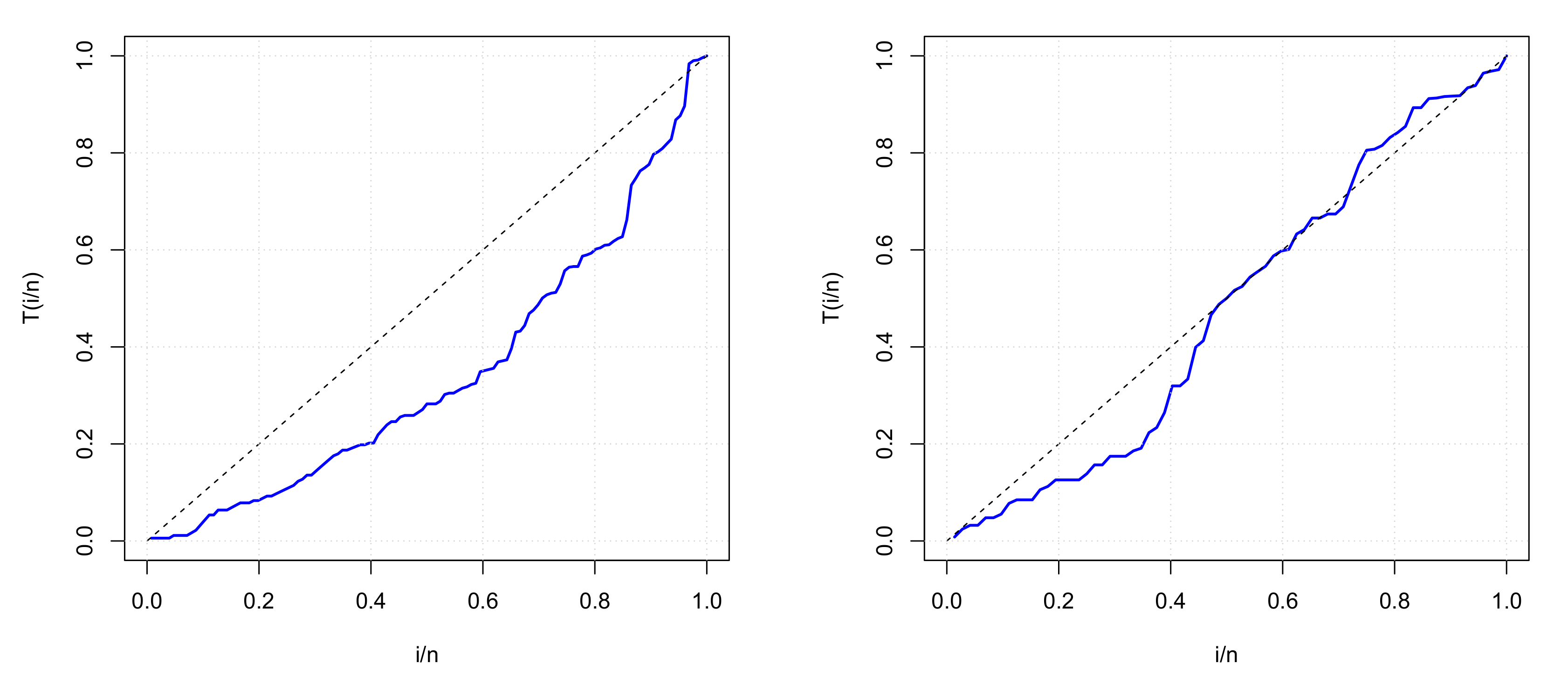
The main observable differences between the two data sets are in the central and dispersion parameters and also, in their right skewed nature: Data set I is highly right skewed whereas Data set II is moderately right skewed. We refine our descriptive analysis by showing the corresponding total time on test (TTT) plots in Figure 5 as introduced by [42].

These TTT plots reveal that Data set I has a concave TTT line, corresponding to a possible subjacent increasing hrf, whereas Data set II has concave-convex TTT line, corresponding to a possible subjacent bathtub-shaped hrf. These two cases are covered by the TOFrE model, motivating its use to analyze such data.

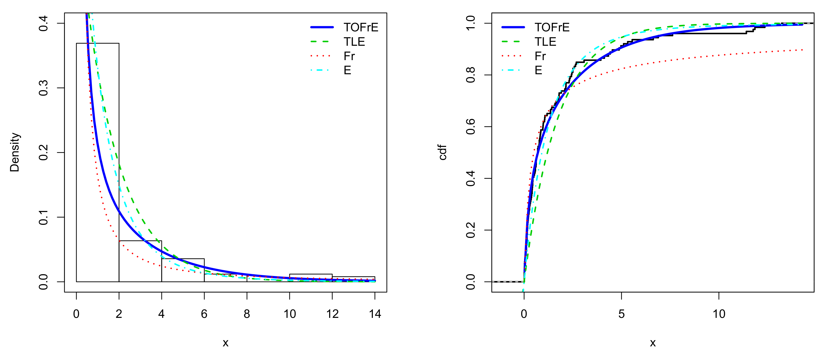
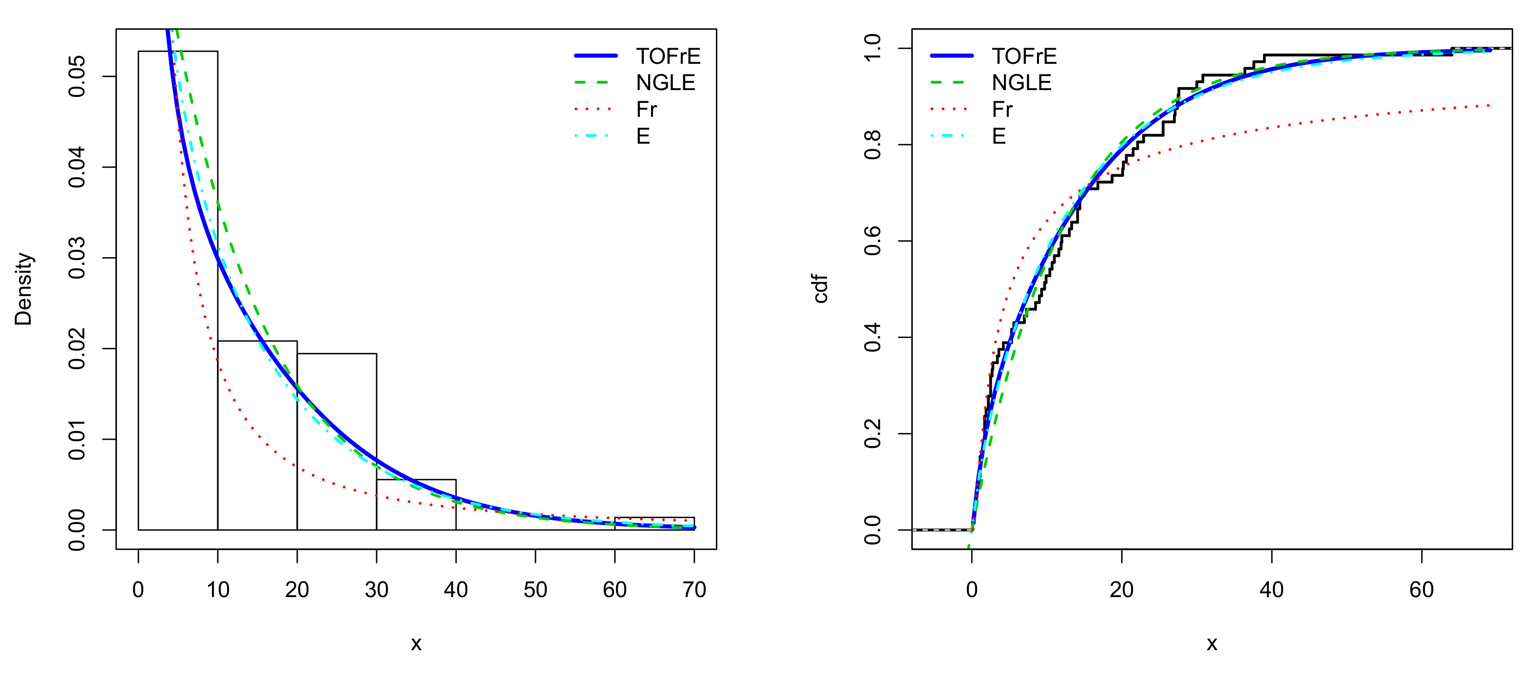
The MLEs of the model’s parameters along with their standard errors (SEs) are collected in

Table 8. Maximum likelihood estimates (MLEs) and standard errors (SEs) of the models for Data set I.

Model	Estimates (MLEs along with Their SEs)
TOFrE	0.7317	0.8173	0.3432
($\lambda ,\beta ,\theta$)	(0.2810)	(0.2433)	(0.0235)
TLE	0.5269	0.0281	0.5375
($\beta ,\theta ,\lambda$)	(0.0817)	(0.0093)	(0.1788)
Fr	0.2538	0.5509
($\alpha ,\theta$)	(0.0436)	(0.0343)
E	0.5794
($\theta$)	(0.0516)

and

Table 9. MLEs and SEs of the models for Data set II.

Model	Estimates (MLEs along with Their SEs)
TOFrE	−0.2624	0.2026	0.4131
($\lambda ,\beta ,\theta$)	(0.2869)	(0.0427)	(0.0490)
NGLE	73.8046	0.0580	0.0953	3.4822
($\alpha ,\beta ,\theta ,\gamma$)	(7.1652)	(0.0153)	(0.0557)	(2.1030)
Fr	2.8798	0.6520
($\alpha ,\theta$)	(0.5533)	(0.0538)
E	0.0819
($\theta$)	(0.0096)

for Data sets I and II, respectively.

Table 10. Numerical measures of fitness of the models for Data set I.

Model	AIC	CVM	AD	KS	KS p-Value
TOFrE	362.5496	0.1244	0.8897	0.0671	0.6215
TLE	373.8305	0.0669	0.4589	0.1070	0.1111
FR	401.8195	0.6067	4.1487	0.1236	0.0425
E	391.5131	0.1767	1.1156	0.1948	0.00014

and

Table 11. Numerical measures of fitness of the models for Data set II.

Model	AIC	CVM	AD	KS	KS p-Value
TOFrE	503.6547	0.0747	0.4277	0.0779	0.7739
NGLE	508.9127	0.1178	0.6623	0.0902	0.6008
FR	538.0378	0.4426	2.5965	0.1531	0.0682
E	506.2559	0.1305	0.7523	0.1422	0.1087

present the values of the criteria of fitness of the models for Data sets I and II, respectively.

From Table 10, we see that the TOFrE and TLE models are the best for Data set I. In particular, the TOFrE model possesses the lowest AIC and KS values, and has the biggest p-value for the KS test; it is the best under these two criteria. From Table 11, the TOFrE model is the best for Data set II; it possesses the lowest AIC, CVM, AD and KS values and has the biggest p-value for the KS test.

Now, we display the plots of the estimated pdfs and cdfs for Data sets I and II in Figure 6 and Figure 7, respectively. Visually, in comparison to the competitor models, the blue curves of the estimated fits of the TOFrE model are more close to the empirical pdfs and cdfs.

We complete this part by determining the confidence intervals of the TOFrE model parameters in

Table 12. Asymptotic two-sided confidence intervals of the TOFrE model parameters at level $90\%$ and $95\%$ for Data sets I and II, respectively.

Confidence Intervals	$\mathit{\lambda }$	$\mathit{\beta }$	$\mathit{\theta }$
$90\%$	[0.2694, 1]	[0.4170, 1.2175]	[0.3045, 0.3818]
$95\%$	[0.1809, 1]	[0.3404, 1.2941]	[0.2974, 0.3892]
Confidence intervals	$\lambda$	$\beta$	$\theta$
$90\%$	[−0.7343, 0.2095]	[0.1323, 0.2728]	[0.3324, 0.4937]
$95\%$	[−0.8247, 0.2999]	[0.1189, 0.2862]	[0.3170, 0.5091]

, as described in Section 4.

5.2. Data Set III (Heavy Tail)

We now consider a data set of different nature from insurance losses, called Data set III. It represents the vehicle insurance losses as considered in [43]. It is fully available at the electronic address: https://chesneau.users.lmno.cnrs.fr/DatasetIII.csv.

We may refer to [43] for all the necessary descriptive statistics. Thus, we aim to apply our statistical methodology to this new data set. As in [43], we also introduced the two following criteria: consistent Akaike information criterion (CAIC), and Hannan–Quinn information criterion (HQIC), which have the same interpretation to the AIC. The MLEs of the considered models are provided in

Table 13. MLEs and SEs of the models for Data set III.

Model	Estimates (MLEs along with Their SEs)
TOFrE	0.5223	0.1163	1.0867
($\lambda ,\beta ,\theta$)	(0.0342)	(0.0016)	(0.0122)
TLE	0.0312	0.0075	0.7629
($\beta ,\theta ,\lambda$)	(0.0014)	(0.00027	(0.0143)
Fr	4.6277	1.8279
($\alpha ,\theta$)	( 0.0279)	(0.0148)
E	0.1249
($\theta$)	(0.0013)

.

Table 14. Numerical measures of fitness of the models for Data set III.

Model	AIC	BIC	CAIC	HQIC	CVM	AD
TOFrE	51,239.82	51,261.18	51,239.82	51,247.08	3.2396	31.2062
TLE	55,344.72	55,366.08	55,344.72	55,351.98	49.78455	303.2997
FR	53,189.52	53,192.11	53,190.52	53,199.52	7.4961	53.22005
E	56,263.67	56,270.79	56,263.67	56,266.09	26.89552	176.5199

indicates the values of the considered criteria of fitness of the models for Data set III.

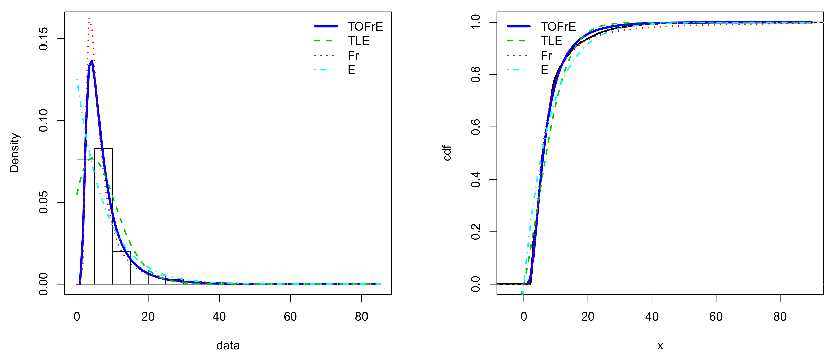
The numerical results in Table 14 show that the TOFrE model provides a better fit to the considered competitors. In addition, for the same data, it is better to the new heavy tailed Weibull (NHTW) model developed by [43], having the following values for the considered criteria: AIC $=67,278.87$, BIC $=67,300.22$, CAIC $=67,281.04$ and HQIC $=67,286.13$ (see [43] (Table 6)), which reveals to be better to other heavy tailed models, such as the Weibull, Kumaraswamy Weibull, Lomax, Marshall–Olkin Weibull and Burr-XII models.

The estimated pdfs and cdfs of the models for Data set III are sketched in Figure 8.

In the light of this study, thanks to all its numerous qualities, we hope that the TOFr-G family will seduce the practitioner for wider applications in applied sciences. As perspectives, the multivariate extensions of the TOFr-G family can be of interest for the construction of various regression models as well as clustering methods, allowing new possibilities for the analysis of big data.

6. Conclusions

In this paper, on the basis of the well-established transmuted-G and odd Fréchet-G families of distributions, we introduce a new family of distribution, called the transmuted odd Fréchet-G (TOFr-G) family. It contains a myriad of new flexible distributions, which can be turned as models to analyze a wide variety of data sets. We treat the theoretical and practical features of the TOFr-G family, with a focus on its member defined with the exponential distribution as baseline. We estimate the model parameters by the maximum likelihood method, showing that it gives convincing results via a simulation study. Then, three practical data sets are analyzed favorably by the proposed model. Among the possible applications, an interesting direction is to study heavy tailed distributions from the TOFr-G family and investigate results related to insurance, as performed in [44,45].

References

- Alzaatreh, A.; Lee, C.; Famoye, F. A new method for generating families of continuous distributions. Metron 2013, 71, 63–79. [Google Scholar] [CrossRef] [Green Version]
- Bantan, R.A.R.; Jamal, F.; Chesneau, C.; Elgarhy, M. Truncated inverted Kumaraswamy generated family of distributions with applications. Entropy 2019, 21, 1089. [Google Scholar] [CrossRef] [Green Version]
- Bourguignon, M.; Silva, R.B.; Cordeiro, G.M. The Weibull-G family of probability distributions. J. Data Sci. 2014, 12, 53–68. [Google Scholar]
- Cordeiro, G.M.; de Castro, M. A new family of generalized distributions. J. Stat. Comput. Simul. 2011, 81, 883–898. [Google Scholar] [CrossRef]
- Gupta, R.D.; Kundu, D. Exponentiated exponential family: An alternative to Gamma and Weibull distributions. Biom. J. 2001, 43, 117–130. [Google Scholar] [CrossRef]
- Eugene, N.; Lee, C.; Famoye, F. Beta-normal distribution and its applications. Commun. Stat. Theory Methods 2002, 31, 497–512. [Google Scholar] [CrossRef]
- Haq, M.A.; Elgarhy, M. The odd Fréchet-G family of probability distributions. J. Stat. Appl. Probab. 2018, 7, 189–203. [Google Scholar] [CrossRef]
- Marshall, A.; Olkin, I. A new method for adding a parameter to a family of distributions with applications to the exponential and Weibull families. Biometrika 1997, 84, 641–652. [Google Scholar] [CrossRef]
- Shaw, W.T.; Buckley, I.R. The Alchemy of Probability Distributions: Beyond Gram-Charlier Expansions, and a Skew-kurtotic-normal Distribution from a Rank Transmutation Map. arXiv 2009, arXiv:0901.0434. [Google Scholar]
- Zografos, K.; Balakrishnan, N. On families of beta- and generalized gamma-generated distributions and associated inference. Stat. Methodol. 2009, 6, 344–362. [Google Scholar] [CrossRef]
- Hameldarbandi, M.; Yilmaz, M. A new perspective of transmuted distribution. Commun. Fac. Sci. Univ. Ank. Ser. A1 Math. Stat. 2019, 68, 1144–1162. [Google Scholar] [CrossRef]
- Yousof, H.M.; Afify, A.Z.; Alizadeh, M.; Butt, N.S.; Hamedani, G.G.; Ali, M.M. The transmuted exponentiated generalized-G family of distributions. Pak. J. Stat. Oper. Res. 2015, 11, 441–464. [Google Scholar] [CrossRef]
- Bakouch, H.; Jamal, F.; Chesneau, C.; Nasir, A. A New Transmuted Family of Distributions: Properties and Estimation with Applications. 2017. Available online: https://hal.archives-ouvertes.fr/hal-01570370v3 (accessed on 1 May 2020).
- Nofal, Z.M.; Afify, A.Z.; Yousof, H. M; Cordeiro, G.M. The generalized transmuted-G family of distributions. Commun. Stat. Theory Methods 2017, 46, 4119–4136. [Google Scholar] [CrossRef]
- Alizadeh, M.; Rasekhi, M.; Yousof, H.M.; Hamedani, G.G. The transmuted Weibull-G family of distributions. Hacet. J. Math. Stat. 2018, 47, 1671–1689. [Google Scholar] [CrossRef]
- Reyad, H.; Jamal, F.; Othman, S.; Hamedani, G.G. The transmuted Odd Lindley-G family of distributions. Asian J. Probab. Stat. 2018, 1, 1–25. [Google Scholar] [CrossRef] [Green Version]
- Alizadeh, M.; Merovci, F.; Hamedani, G.G. Generalized transmuted family of distributions: Properties and applications. Hacet. J. Math. Stat. 2017, 46, 645–667. [Google Scholar] [CrossRef]
- Reyad, H.; Jamal, F.; Othman, S.; Hamedani, G.G. The transmuted Gompertz-G family of distributions: Properties and applications. Tbil. Math. J. 2018, 11, 47–67. [Google Scholar] [CrossRef]
- Jayakumar, K.; Babu, M.G. T-transmuted X family of distributions. Statistica 2017, 77, 251–276. [Google Scholar]
- Mansour, M.M.; Abd Elrazik, E.M.; Afify, A.Z.; Ahsanullah, M.; Altun, E. The transmuted transmuted-G family: Properties and applications. J. Nonlinear Sci. Appl. 2019, 12, 217–229. [Google Scholar] [CrossRef]
- Reyad, H.; Othman, S.; Ul Haq, M.A. The transmuted generalized odd generalized exponential-G family of distributions: Theory and applications. J. Data Sci. 2019, 17, 279–300. [Google Scholar]
- Alrajhi, S. The odd Fréchet inverse exponential distribution with application. J. Nonlinear Sci. Appl. 2019, 12, 535–542. [Google Scholar] [CrossRef] [Green Version]
- Nasiru, S. Extended odd Fréchet-G family of distributions. J. Probab. Stat. 2018, 1, 1–12. [Google Scholar] [CrossRef]
- Reyad, H.; Karkmaz, M.C.; Afify, A.Z.; Hamedani, G.G.; Othman, S. The Fréchet Topp Leone-G family of distributions: Properties, characterizations and applications. Ann. Data Sci. 2019. [Google Scholar] [CrossRef]
- Chesneau, C.; Djibrila, S. The generalized odd inverted exponential-G family of distributions: Properties and applications. Eurasian Bull. Math. 2019, 2, 86–110. [Google Scholar]
- Yousof, H.M.; Rasekhi, M.; Altun, E.; Alizadeh, M. The extended odd Fréchet family of distributions: Properties, applications and regression modeling. Int. J. Math. Comput. 2019, 30, 1–16. [Google Scholar]
- Tian, Y.; Tian, M.; Zhu, Q. Transmuted linear exponential distribution: A new generalization of the linear exponential distribution. Commun. Stat. Simul. Comput. 2014, 43, 2661–2677. [Google Scholar] [CrossRef]
- Tian, Y.; Tian, M.; Zhu, Q. A new generalized linear exponential distribution and its applications. Acta Math. Appl. Sin. Engl. Ser. 2014, 30, 1049–1062. [Google Scholar] [CrossRef]
- Klein, J.P.; Moeschberger, M.L. Survival Analysis: Techniques for Censored and Truncated Data, 2nd ed.; Springer: Cham, Switzerland, 2003. [Google Scholar]
- Lindley, D.V. Fiducial distributions and Bayes theorem. J. R. Stat. Soc. A 1958, 20, 102–107. [Google Scholar] [CrossRef]
- Lindley, D.V. Introduction to Probability and Statistics from a Bayesian Viewpoint, Part II: Inference; Cambridge University Press: New York, NY, USA, 1965. [Google Scholar]
- Lomax, K.S. Business Failures; Another example of the analysis of failure data. J. Am. Stat. Assoc. 1954, 49, 847–852. [Google Scholar] [CrossRef]
- Cordeiro, G.M.; Silva, R.B.; Nascimento, A.D.C. Recent Advances in Lifetime and Reliability Models; Bentham Books: Sharjah, UAE, 2020. [Google Scholar]
- Kenney, J.F.; Keeping, E.S. Mathematics of Statistics, 3rd ed.; Van Nostrand: Princeton, NJ, USA, 1962; Pt. 1; p. 101. [Google Scholar]
- Moors, J.J.A. A quantile alternative for kurtosis. J. R. Stat. Soc. Ser. D (Stat.) 1988, 37, 25–32. [Google Scholar] [CrossRef] [Green Version]
- Gupta, P.L.; Gupta, R.C. On the moments of residual life in reliability and some characterization results. Commun. Stat. Theory Methods 1983, 12, 449–461. [Google Scholar] [CrossRef]
- Lai, C.D.; Xie, M. Stochastic Aging and Dependence for Reliability; Springer: New York, NY, USA, 2006. [Google Scholar]
- Polisicchio, M.; Porro, F. A comparison between Lorenz L(p) curve and Zenga I(p) curve. Stat. Appl. 2009, 21, 289–301. [Google Scholar]
- Casella, G.; Berger, R.L. Statistical Inference, Duxbury Advanced Series; Thomson Learning: Pacific Grove, CA, USA, 2002. [Google Scholar]
- Coetzee, J.L. Reliability degradation and the equipment replacement problem. In Proceedings of the International Conference of Maintenance Societies (ICOMS 96), Melbourne, Australia, 22 May 1996. [Google Scholar]
- Choulakian, V.; Stephens, M.A. Goodness-of-fit for the generalized Pareto distribution. Technometrics 2001, 43, 478–484. [Google Scholar] [CrossRef]
- Aarset, M.V. How to identify bathtub hazard rate. IEEE Trans. Reliab. 1987, 36, 106–108. [Google Scholar] [CrossRef]
- Ahmad, Z.; Mahmoudi, E.; Dey, S. A new family of heavy tailed distributions with an application to the heavy tailed insurance loss data. Commun. Stat. Simul. Comput. 2020. [Google Scholar] [CrossRef]
- Gómez-Déniz, E.; Calderín-Ojeda, E. A Suitable Alternative to the Pareto Distribution. Hacet. J. Math. Stat. 2014, 43, 843–860. [Google Scholar]
- Gómez-Déniz, E.; Calderín-Ojeda, E. Modeling insurance data with the Pareto ArcTan distribution. ASTIN Bull. 2015, 45, 639–660. [Google Scholar] [CrossRef]
Figure 1.
A panel of shapes for the pdf of the transmuted odd Fréchet exponential (TOFrE) distribution.
Figure 2.
A panel of shapes for the hrf of the TOFrE distribution.
Figure 3.
Individual plots of the hazard rate function (hrf) of the TOFrE distribution for the main observed shapes.
Figure 4.
Box plots for Data sets I and II, respectively.
Figure 5.
Total time on test (TTT) plots for Data sets I and II, respectively.
Figure 6.
Plots of all the estimated pdfs and cdfs for Data set I.
Figure 7.
Plots of all the estimated pdfs and cdfs for Data set II.
Figure 8.
Plots of all the estimated pdfs and cdfs for Data set III.