Joint-Space Characterization of a Medical Parallel Robot Based on a Dual Quaternion Representation of SE(3)

 , ,
, , 
Abstract
:1. Introduction
2. Materials and Methods
2.1. The Study Parameters of SE(3)
2.2. Joint Space Caracterization
- (1)
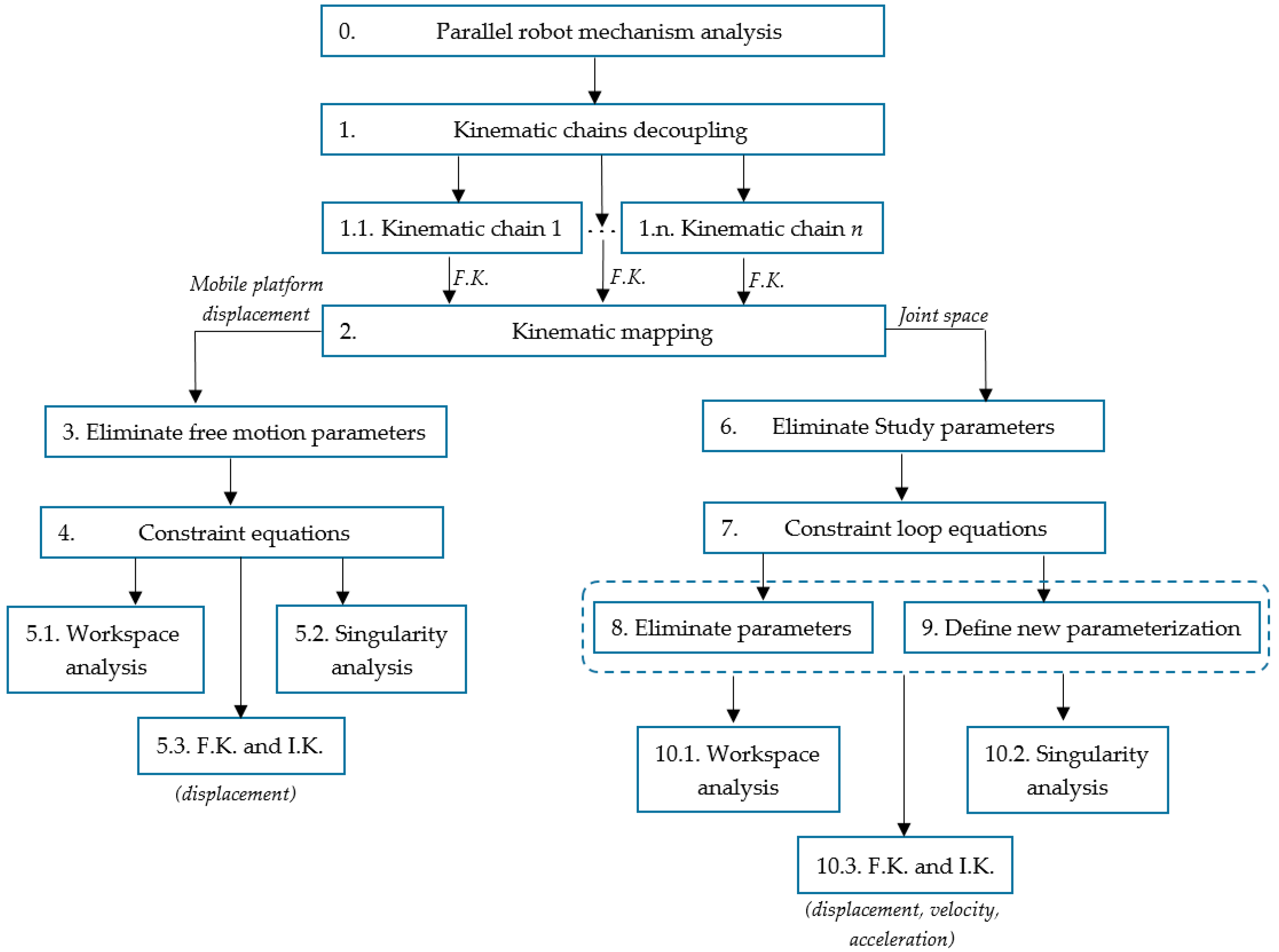
- The description of the joint space where certain dependencies are obtained: the method is suitable for applications were these dependencies are more important than the motion of a mobile platform (e.g., rehabilitation using exoskeletons based on a parallel mechanism). Furthermore, the constraints may be used in velocity and acceleration kinematics and also reveal the singularities of the mechanism.
- (2)
- The loop constraints may be used in defining new parameterizations e.g., assigning coordinate systems at any element in the mechanism (which is presented on a case study in Section 3).
2.3. Defining New Motion Parameterizations Based on the Joint-Space Characterization
- define the input motion parameters (the actuated joints denoted qi); at this point the passive joints and the active ones should be established;
- define the fixed coordinate frame and the mobile one, respectively; the fixed coordinate frame XYZ is defined as being attached to a chosen base and the mobile coordinate frame X’Y’Z’ is attached to the chosen mobile platform;
- define a mechanical “path” (denoted P, composed of joints and links), which connects the fixed frame with the mobile one; usually the shortest path yields the simpler equations, however it is not mandatory to define the shortest path (as it is illustrated in the example shown in Section 2.3);
- determine the motion parameters (denoted ai) within P;
- eliminate the unwanted motion parameters (denoted bi); the parameters bi are all the motion parameters that are not qi or ai;
- express the ai parameters with respect to the input parameters qi (fi represents an irrational function of the active joints qi):
- create a geometric parameterization of P; one example is to use the Denavit-Hartenberg convention; and,
- substitute ai into P; at this point, the relative displacement between the fixed coordinate frame XYZ and the mobile one X’Y’Z’ (with respect to the input parameters qi) is achieved. Consequently, the constraints of the mechanism are obtained vis-à-vis the newly defined parameterization.
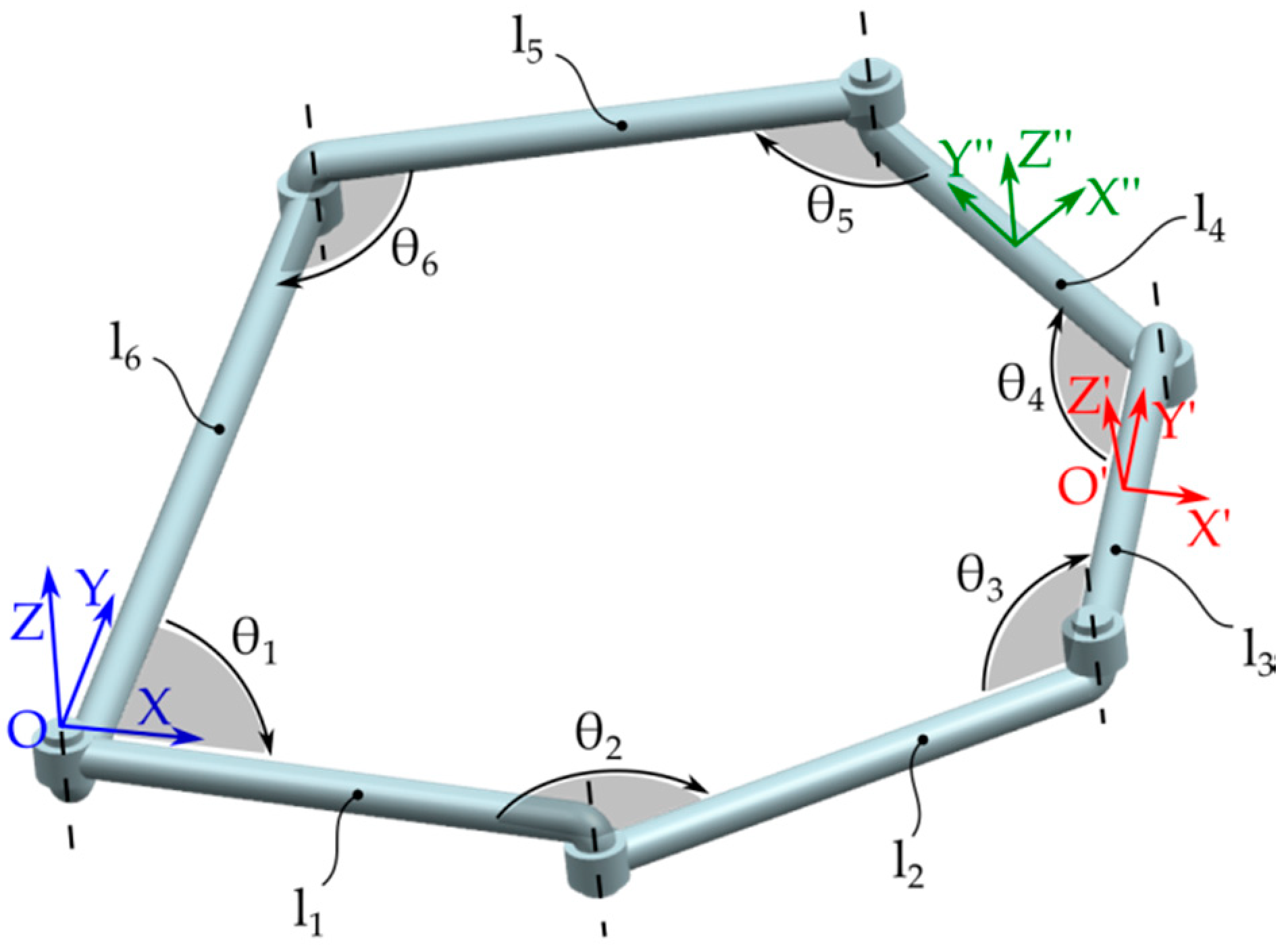
2.4. Joint Space Characterization of a 6-R Closed Loop Planar Parallel Mechanism
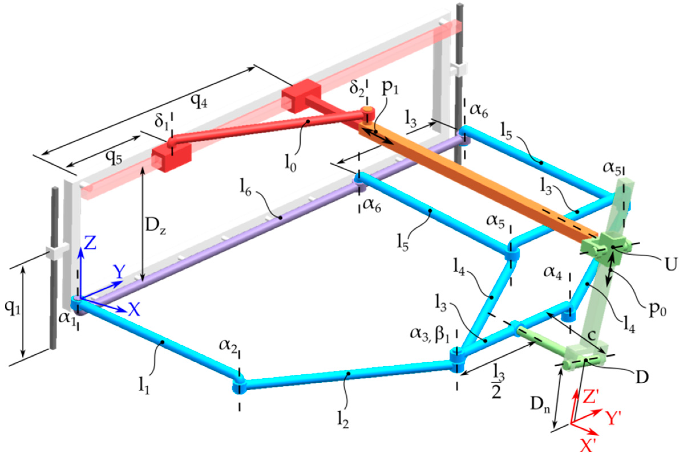
3. PRO-HEP-LCT Kinematics (a Case Study)
- the upper planar mechanism, which is a PRR-PP mechanism (prismatic-revolute-revolute chain coupled with a prismatic-prismatic chain where the underline represents the actuated joint). The upper planar mechanism creates two DOF pure translational motion (actuated by q4 and q5) in a plane parallel to XY plane;
- the lower planar chain, which is a 6R-3R mechanism, i.e., a 6R closed loop planar chain coupled with a 3R chain which creates pure translational 2 DOF motion (actuated by q2 and q3) in the XY plane; in the parameterization α1 and α6 are the tangent of half angles of the q2 and q3 active joint, respectively; and,
- the mobile platform, is a UPU mechanism with a prismatic joint in-between two universal joints which are connected to the upper and the lower planar mechanisms, respectively.
3.1. Joint Space Caracterization of the PRO-HEP-LCT Parallel Robotic System
3.1.1. The Lower Planar Mechanism
3.1.2. The Upper Planar Mechanism
3.1.3. The Mobile Platform Mechanism
3.2. Velocity Kinematics of the PRO-HEP-LCT Parallel Robotic System
3.3. Acceleration Kinematics of the PRO-HEP-LCT Parallel Robotic System
4. Numerical Results
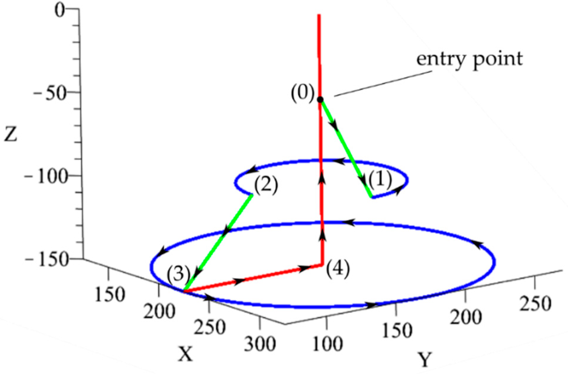
- the initial conditions are defined by the entry point (0) (see Figure 5) that has the Cartesian coordinates [X = 225, Y = 170, Z = 0] (dimensions in mm) where the US probe has the orientation [ϕ1 = 0°, ϕ1 = 45°] (dimensions in angular degrees);
- the entry point is defined as a Remote Center of Motion (RCM) point;
- the probe is inserted from point (0) to point (1) until it reaches Z = −50 by actuating the redundant DOF described by the Dn parameter;
- the tip of the probe is guided on a circular path (counter-clockwise direction) until it reaches the point (2) (a rotation of 3π/2);
- the probe is further inserted on a linear trajectory until it reaches the point (3) at Z = −100;
- the tip of the probe is guided on a full circle (counter-clockwise direction), from point (3) back to point (3);
- the tip of the probe is guided on a linear trajectory until it reaches the point (4); at this point, the tip of the probe has the Cartesian coordinates [X = 225, Y = 170, Z = −100] and the orientations [ϕ1 = 0°, ϕ1 = 0°]; and,
- the probe is retracted from the patients’ body.
5. Discussion
6. Conclusions
Author Contributions
Funding
Conflicts of Interest
References
- Klug, C.; Schmalstieg, D.; Gloor, T. A Complete Workflow for Automatic Forward Kinematics Model Extraction of Robotic Total Stations Using the Denavit-Hartenberg Convention. J. Intell Robot. Syst. 2019, 95, 311–329. [Google Scholar] [CrossRef] [Green Version]
- Faria, C.; Vilaça, J.L.; Monteiro, S.; Erlhagen, W.; Bicho, E. Automatic Denavit-Hartenberg Parameter Identification for Serial Manipulators. In Proceedings of the IECON 2019—45th Annual Conference of the IEEE Industrial Electronics Society, Lisbon, Portugal, 14–17 October 2019. [Google Scholar]
- Zhang, J.; Lian, B.; Song, Y. Geometric error analysis of an over-constrained parallel tracking mechanism using the screw theory. Chin. J. Aeronaut. 2019, 32, 1541–1554. [Google Scholar] [CrossRef]
- Yin, F.W.; Tian, W.J.; Liu, H.T.; Huang, T.; Chetwynd, D.G. A screw theory based approach to determining the identifiable parameters for calibration of parallel manipulators. Mech. Mach. Theory 2020, 145, 103665. [Google Scholar] [CrossRef]
- Angeles, J. Fundamentals of Robotic Mechanical Systems. In Theory Methods Algorithms; Springer: Berlin/Heidelberg, Germany, 2014; ISSN 978-3-319-01850-8. [Google Scholar]
- Husty, M.; Pfurner, M.; Schrocker, H.P.; Brunnthaler, K. Algebraic Methods in Mechanism Analysis and Synthesis. Robotica 2007, 25, 661–675. [Google Scholar] [CrossRef] [Green Version]
- Müller, A. An overview of formulae for the higher-order kinematics of lower-pair chains with applications in robotics and mechanism theory. Mech. Mach. Theory 2019, 142, 103594. [Google Scholar] [CrossRef]
- Husty, M.L.; Walter, D.R. Mechanism Constraints and Singularities—The Algebraic Formulation. In Singular Configurations of Mechanisms and Manipulators. CISM International Centre for Mechanical Sciences (Courses and Lectures); Müller, A., Zlatanov, D., Eds.; Springer: Berlin/Heidelberg, Germany, 2019. [Google Scholar]
- Sun, T.; Yang, S.; Lian, B. Finite and Instantaneous Screw Theory. Finite and Instantaneous Screw Theory in Robotic Mechanism; Springer Tracts in Mechanical Engineering; Springer: Singapore, 2020. [Google Scholar]
- Lin, P.; Huang, M.; Huang, H. Analytical Solution for Inverse Kinematics Using Dual Quaternions. IEEE Access 2019, 7, 166190–166202. [Google Scholar] [CrossRef]
- Pisla, D.; Birlescu, I.; Vaida, C.; Tucan, P.; Pisla, A.; Gherman, B.; Crisan, N.; Plitea, N. Algebraic modeling of kinematics and singularities for a prostate biopsy parallel robot. Proc. Rom. Acad. Ser. A 2018, 19, 489–497. [Google Scholar]
- Birlescu, I.; Vaida, C.; Pisla, A.; Carbone, G.; Pisla, D. Singularity Analysis of a Spherical Robot Used in Upper Limb Rehabilitation. Interdiscip. Appl. Kinemat. Mech. Mach. Sci. 2019, 71, 205–213. [Google Scholar]
- Birlescu, I. Studies Regarding the Safe Operation of Innovative Medical Parallel Robots. Ph.D. Thesis, Technical University of Cluj-Napoca, Cluj-Napoca, Romania, 2019. [Google Scholar]
- Ge, Q.J.; McCarthy, J.M. An Algebraic Formulation of Configuration-Space Obstacles for Spatial Robots. Proc. IEEE Int. Conf. Robot. Autom. 1990, 3, 1542–1547. [Google Scholar]
- Husty, M.; Birlescu, I.; Tucan, P.; Vaida, C.; Pisla, D. An algebraic parameterization approach for parallel robots analysis. Mech. Mach. Theory 2019, 140, 245257. [Google Scholar] [CrossRef]
- Chablat, D.; Rouillier, F.; Moroz, G. Workspace and joint space analysis of the 3-rps parallel robot. In Proceedings of the ASME 2014 International Design Engineering Technical Conferences & Computers and Information in Engineering Conference IDETC/CIE 2014, Buffalo, NY, USA, 17–20 August 2014. [Google Scholar]
- Pisla, D.; Birlescu, I.; Vaida, C.; Gherman, B.; Tucan, P.; Carbone, G.; Plitea, N. Parallel Robot for Lower Limb Rehabilitation. Patent Pending A/00334/04.06.2019, 4 June 2019. [Google Scholar]
- Pisla, D.; Gherman, B.; Nadas, I.; Pop, N.; Craciun, F.; Tucan, P.; Vaida, C.; Carbone, G. Innovative Parallel Robot for Lower Limb Rehabilitation. Patent Pending A00391/27.06.2019, 27 June 2019. [Google Scholar]
- Gherman, B.; Birlescu, I.; Plitea, N.; Carbone, G.; Tarnita, D.; Pisla, D. On the singularity-free workspace of a parallel robot for lower-limb rehabilitation. Proc. Rom. Acad. 2019, 20, 383–391. [Google Scholar]
- Vaida, C.; Birlescu, I.; Pisla, A.; Ulinici, I.; Tarnita, D.; Carbone, G.; Pisla, D. Systematic Design of a Parallel Robotic System for Lower Limb Rehabilitation. IEEE Access 2020, 8, 34522–34537. [Google Scholar] [CrossRef]
- Merlet, J.P. Parallel Robots. In Solid Mechanics and Its Applications; Springer: Berlin/Heidelberg, Germany, 2006; ISBN 978-1-4020-4133-4. [Google Scholar]
- Rangaprasad, A.S.; Sandipan, B. Analysis of Constraint Equations and Their Singularities. Adv. Robot Kinemat. 2014, 429–436. [Google Scholar] [CrossRef]
- Cox, D.; Little, J.; O’Shea, D. Ideals, Varieties and Algorithms. In An Introduction to Computational Algebraic Geometry and Commutative Algebra, 4th ed.; Springer: Berlin/Heidelberg, Germany, 2015; ISBN 978-3-319-16720-6. [Google Scholar]
- Birlescu, I.; Husty, M.; Vaida, C.; Gherman, B.; Ulinici, I.; Bogateanu, R.; Pisla, D. Motion parameterization of parallel robots used in lower limb rehabilitation. Adv. Robot Kinemat. 2020, in press. [Google Scholar]
- Plitea, N.; Pisla, D.; Vaida, C.; Gherman, B.; Tucan, P. Pro-Hep-LCT- Parallel robot for the minimally invasive treatment of hepatic carcinoma. Patent pending A1017/03.12.2018, 3 December 2018. [Google Scholar]
- Birlescu, I.; Husty, M.; Vaida, C.; Plitea, N.; Nayak, A.; Pisla, D. Complete Geometric Analysis Using the Study SE(3) Parameters for a Novel, Minimally Invasive Robot Used in Liver Cancer Treatment. Symmetry 2019, 11, 1491. [Google Scholar] [CrossRef] [Green Version]
- Gherman, B.; Birlescu, I.; Burz, A.; Pisla, D. Kinematic analysis of two innovative medical instruments for the robotic assisted treatment of non-resectable liver tumors. EUCOMES 2020, in press. [Google Scholar]
- Birlescu, I.; Gherman, B.; Burz, A.; Pisla, D. Automated medical instrument with multiple parallel needles for the intersitital brachytherapy. Patent pending A00710/06.11.2019, 6 November 2019. [Google Scholar]
- Birlescu, I.; Vaida, C.; Gherman, B.; Burz, A.; Tucan, P.; Plitea, N.; Pisla, D. Automated medical instrument for the manipulation of a laparoscopic ultasound probe. Unpublished patent 2020. [Google Scholar]
- Oliveira, A.S.; De Pieri, E.R.; Moreno, U.F. A new method of applying differential kinematics through dual quaternions. Robotica 2017, 35, 907–921. [Google Scholar] [CrossRef]
- Yang, X.L.; Wu, H.T.; Li, Y.; Kang, S.Z.; Chen, B. Computationally Efficient Inverse Dynamics of a Class of Six-DOF Parallel Robots: Dual Quaternion Approach. J. Intell. Robot. Syst. 2019, 94, 101–113. [Google Scholar] [CrossRef]
- Marinho, M.M.; Figueredo, L.F.C.; Adorno, B.V. A Dual Quaternion Linear-Quadratic Optimal Controller for Trajectory Tracking. In Proceedings of the 2015 IEEE/RSJ International Conference on Intelligent Robots and Systems (IROS), Hamburg, Germany, 28 September–2 October 2015. [Google Scholar]
- Vaida, C.; Plitea, N.; Al Hajjar, N.; Burz, A.; Graur, F.; Pisla, D. A new robotic assisted approach in minimally invasive treatment of liver tumours. Proc. Rom. Acad. Ser. A 2020, in press. [Google Scholar]
- Pisla, D.; Plitea, N.; Gherman, B.G.; Vaida, C.; Pisla, A.; Suciu, M. Kinematics and Design of a 5-DOF Parallel Robot Used in Minimally Invasive Surgery. In Advances in Robot Kinematics: Motion in Man and Machine; Springer: Berlin/Heidelberg, Germany, 2010. [Google Scholar]
- Pisla, D.; Plitea, N.; Vaida, C. Kinematic Modeling and Workspace Generation for a New Parallel Robot Used in Minimally Invasive Surgery. In Advances in Robot Kinematics: Analysis and Design; Springer: Berlin/Heidelberg, Germany, 2008. [Google Scholar]
- Pisla, D.; Gherman, B.; Plitea, N. PARASURG hybrid parallel robot for minimally invasive surgery. Chirurgia 2011, 106, 619–625. [Google Scholar]
- Plitea, N.; Pisla, D.; Vaida, C.; Gherman, B.; Szilaghyi, A.; Galdau, B.; Cocorean, D.; Covaciu, F. On the kinematics of a new parallel robot for brachytherapy. Proc. Rom. Acad. Ser. A 2014, 15, 354–361. [Google Scholar]
- Vaida, C.; Pisla, D.; Schadlbauer, J.; Husty, M.; Plitea, N. Kinematic Analysis of an Innovative Medical Parallel Robot Using Study Parameters. In New Trends in Medical and Service Robots: Human Centered Analysis, Control and Design, Mechanisms and Machine Science; Springer International Publishing: Cham, Switzerland, 2016; Volume 39, pp. 85–99. [Google Scholar]
- Gherman, B.; Vaida, C.; Pisla, D.; Plitea, N.; Gyurka, B.; Lese, D.; Glogoveanu, M. Singularities and workspace analysis for a parallel robot for minimally invasive surgery. In Proceedings of the 2010 IEEE International Conference on Automation, Quality and Testing, Robotics, Washington, DC, USA, 28–30 May 2010; pp. 319–324. [Google Scholar]
- Tarnita, D.; Pisla, D.; Geonea, I.; Vaida, C.I. Static and Dynamic Analysis of Osteoarthritic and Orthotic Human Knee. J. Bionic. Eng. 2019, 16, 514–525. [Google Scholar] [CrossRef]


| Symbol | Explicit form | Details |
|---|---|---|
| Q1(θ1) | [1:0:0:α1:0:0:0:0] | θ1 = π/2 → α1 = 0 1 |
| Q2(l1) | [1:0:0:0:0:−l1/2:0:0] | translation along OX |
| Q3(θ2) | [1:0:0:α2:0:0:0:0] | θ2 = π → α2 = 0 1 |
| Q4(l2) | [1:0:0:0:0:−l2/2:0:0] | translation along OX |
| Q5(θ3) | [1:0:0:α3:0:0:0:0] | θ3 = π/2 → α3 = 0 1 |
| Q6(l3/2) | [1:0:0:0:0:0:−l3/4:0] | translation along OY |
| Q7(l6) | [1:0:0:0:0:0:−l6/2:0] | translation along OY |
| Q8(θ6) | [1:0:0:α6:0:0:0:0] | θ6 = π/2 → α6 = 0 1 |
| Q9(l5) | [1:0:0:0:0:−l5/2:0:0] | translation along OX |
| Q10(θ5) | [1:0:0:α5:0:0:0:0] | θ5 = π → α5 = 0 1 |
| Q11(l4) | [1:0:0:0:0:−l4/2:0:0] | translation along OX |
| Q12(θ4) | [1:0:0:α4:0:0:0:0] | θ4 = π/2 → α4 = 0 1 |
| Q13(-l3/2) | [1:0:0:0:0:0:l3/4:0] | translation along OY |
| I-O | Symbol | Value | Assoc. Angle (°) |
|---|---|---|---|
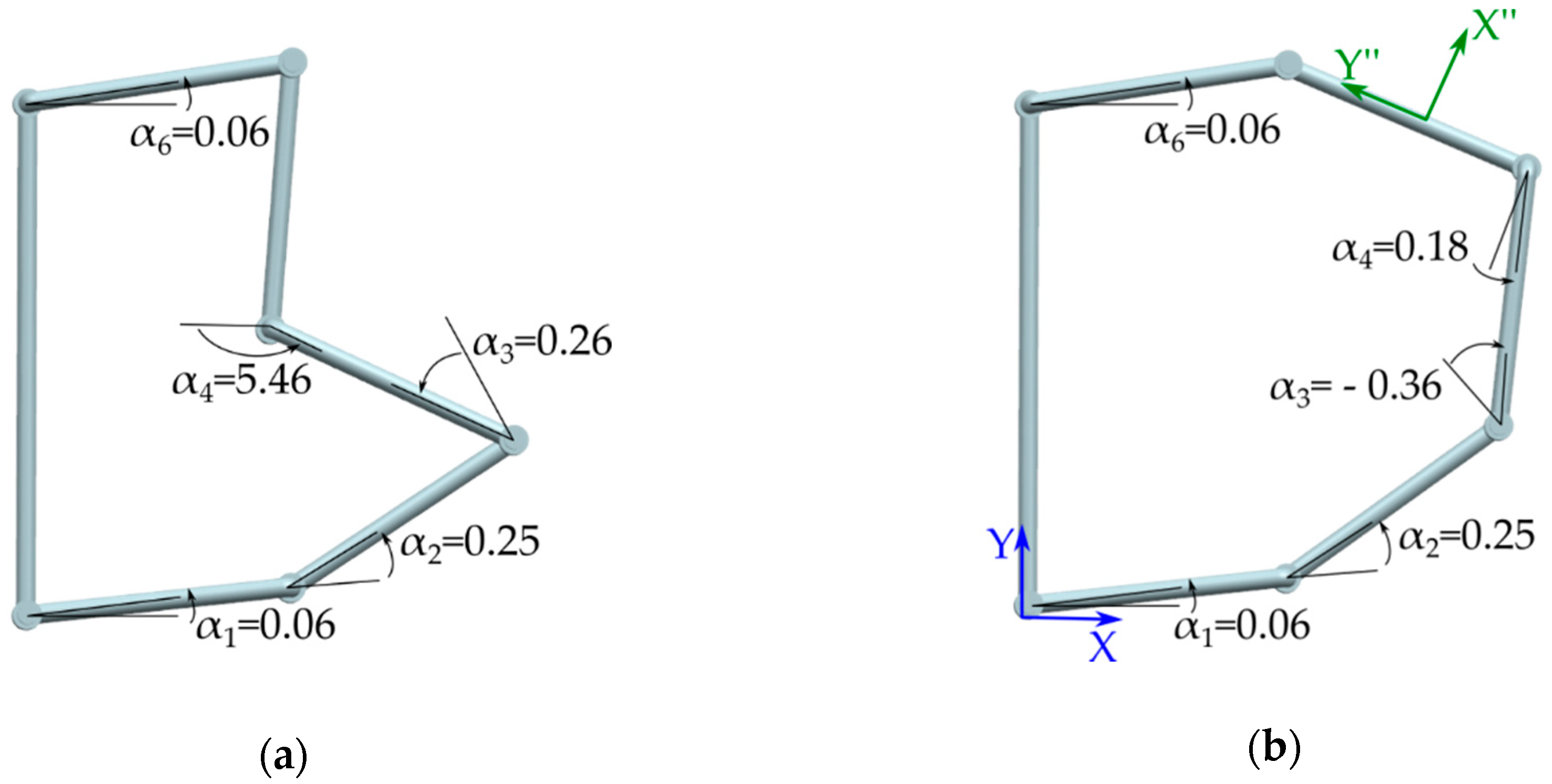
| I | α1 | 0.06 | θ1 = 6.9 |
| α2 | 0.25 | θ2 = 28.1 | |
| α6 | 0.06 | θ6 = 6.9 | |
| O | α3 | 0.26; −0.36 | θ3 = 29.5; θ3 = −39.7 |
| α4 | 5.46; 0.18 | θ4 = 159.2; θ4 = 20.8 |
| Symbol | Explicit form | Details |
|---|---|---|
| Q21(Dz) | [1:0:0:0:0:0:0:−Dz/2] | (geometric) translation along OZ |
| Q22(q5) | [1:0:0:0:0:0:−q5/2:0] | (active)translation along OY |
| Q23(δ1) | [1:0:0:δ1:0:0:0:0] | (passive)rotation about OZ |
| Q24(l0) | [1:0:0:0:0:−l0/2:0:0] | (geometric) translation along OX |
| Q25(δ2) | [1:0:0:δ2:0:0:0:0] | (passive) rotation about OZ |
| Q26(l0) | [1:0:0:0:0:0:0:−Dz/2] | (geometric) translation along OZ |
| Q27(q4) | [1:0:0:0:0:0:−q4/2:0] | (active)translation along OY |
| Q28(p1) | [1:0:0:0:0:−p1/2:0:0] | (free) translation along OX |
| Symbol | Explicit form | Details |
|---|---|---|
| Q29(Xd) | [1:0:0:0:0:−Xd/2:0:0] | (active) translation along OX |
| Q30(Yd) | [1:0:0:0:0:0:−Yd/2:0] | (active) translation along OY |
| Q31(c) | [1:0:0:0:0:−c/2:0:0] | (geometric) translation along OX |
| Q32(φ1) | [1:φ1:0:0:0:0:0:0] | (passive) rotation about OX |
| Q33(φ2) | [1:0:φ2:0:0:0:0:0] | (passive) rotation about OY |
| Q34(Dn) | [1:0:0:0:0:0:0:Dn/2] | (active) translation along OZ |
| Q35(Dz) | [1:0:0:0:0:0:0:−Dz/2] | (geometric) translation along OZ |
| Q36(Xu) | [1:0:0:0:0:−Xu/2:0:0] | (active) translation along OX |
| Q37(Yd) | [1:0:0:0:0:0:−Yu/2:0] | (active) translation along OY |
| Q38(λ1) | [1:λ1:0:0:0:0:0:0] | (passive) rotation about OX |
| Q39(λ2) | [1:0:λ2:0:0:0:0:0] | (passive) rotation about OY |
| Q40(p0) | [1:0:0:0:0:0:0:−p0/2] | (pasive) translation along OZ |
| Q41(Dn) | [1:0:0:0:0:0:0:Dn/2] | (active) translation along OZ |
© 2020 by the authors. Licensee MDPI, Basel, Switzerland. This article is an open access article distributed under the terms and conditions of the Creative Commons Attribution (CC BY) license (http://creativecommons.org/licenses/by/4.0/).
Share and Cite
Birlescu, I.; Husty, M.; Vaida, C.; Gherman, B.; Tucan, P.; Pisla, D. Joint-Space Characterization of a Medical Parallel Robot Based on a Dual Quaternion Representation of SE(3). Mathematics 2020, 8, 1086. https://0-doi-org.brum.beds.ac.uk/10.3390/math8071086
Birlescu I, Husty M, Vaida C, Gherman B, Tucan P, Pisla D. Joint-Space Characterization of a Medical Parallel Robot Based on a Dual Quaternion Representation of SE(3). Mathematics. 2020; 8(7):1086. https://0-doi-org.brum.beds.ac.uk/10.3390/math8071086
Chicago/Turabian StyleBirlescu, Iosif, Manfred Husty, Calin Vaida, Bogdan Gherman, Paul Tucan, and Doina Pisla. 2020. "Joint-Space Characterization of a Medical Parallel Robot Based on a Dual Quaternion Representation of SE(3)" Mathematics 8, no. 7: 1086. https://0-doi-org.brum.beds.ac.uk/10.3390/math8071086