Probabilistic Study of the Effect of Anti-Epileptic Drugs Under Uncertainty: Cost-Effectiveness Analysis

Abstract

Epilepsy is one of the most ancient diseases. Despite the efforts of scientists and doctors to improve the quality of live of epileptic patients, the disease is still a mystery in many senses. Anti-epileptic drugs are fundamental to reduce epileptic seizures but it have some adverse effects, which influence the quality of life outcomes of the patients. In this paper, we study the effectiveness of anti-epileptic drugs taking into account the inherent uncertainty. We establish a model, which allows to represent the natural history of epilepsy, using Markov chains. After randomizing the mathematical model, we compute the first probability density function of the solution stochastic process applying the random variable transformation technique. We also take advantage of this method to determine the distribution of some key quantities in medical decision, such as the time until a certain proportion of the population remains in each state and the incremental cost-effectiveness ratio. The study is completed computing all these quantities using data available in the literature. In addition, regarding the incremental cost-effectiveness ratio, different third generation anti-epileptic treatments are compared with the Brivaracetam, a new third generation anti-epileptic drug.

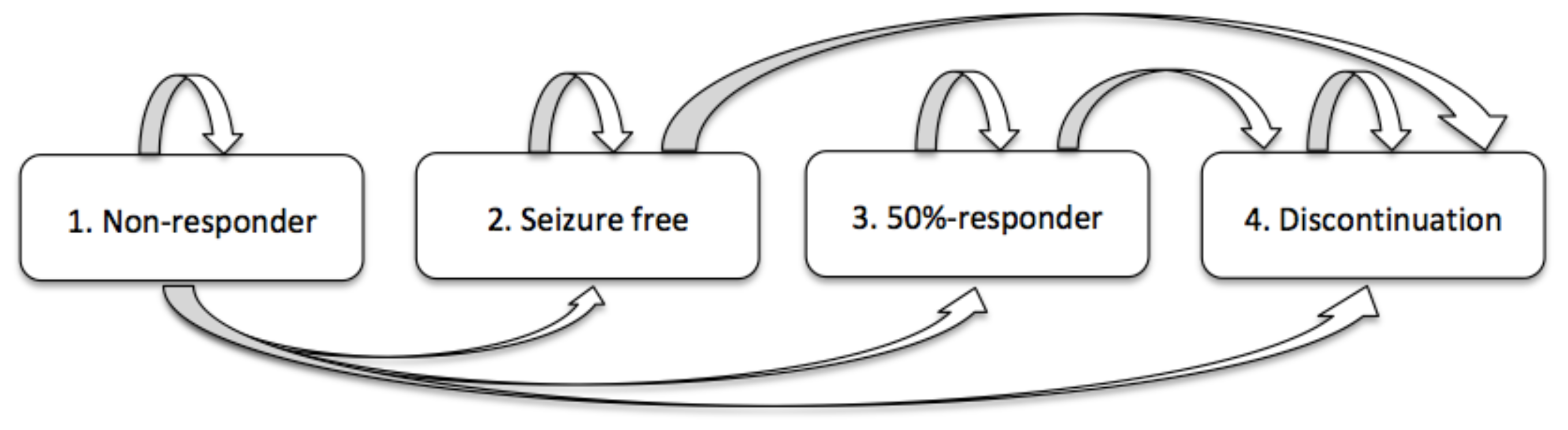
1. Motivation and Preliminaries

From 2000 B.C., multiple reports of epileptic seizures can be found [1]. Thus, epilepsy can be considered one of the most ancient diseases that we have knowledge. Nowadays, there is further awareness about this disease and with that more maintenance of the patients’ lives. Although patients can have much more quality of life, the disease is still a mystery in many senses. Then, it is essential to study it in greater depth. In short, epilepsy is a chronic brain disorder, characterized mainly by epileptic seizures, which are intermittent and unpredictable interruptions of normal brain function. These epileptic seizures are caused by abnormalities in the electrical signals in certain areas of the brain. Groups of neurons suddenly emit disorganized electrical signals, resulting in seizures and other strange symptoms and sensations that can lead to loss of consciousness [2].

Epilepsy is one of the most frequent chronic neurological diseases in the world. The World Health Organization estimates that it affects some 50 million people, a figure that is considerably higher if we contextualize it with Parkinson’s or dementia, which affects approximately 10 and 36 million people, respectively [3]. In Spain, it is estimated that around 370,000 people are affected [2,4]. There are two types of epileptic seizures, generalized seizures in which the epileptic discharge affects the entire surface of the brain at the same time and the partial or focal seizures in which the discharge begins in a part of the brain, nearly 60% of patients having partial-onset seizures [5]. Not everyone experiences all symptoms which may include: abnormal stiffness of the arm and/or leg; illusions and hallucinations; or confusion/exhaustion following cessation of seizure, among others. Anti-epileptic drugs (AEDs) effect is centred in reducing the quantity of epileptic seizures while minimizing long-term toxicity and adverse effects as far as possible [6].

The treatment of epilepsy is mainly performed with AEDs. At present, there are multiple AEDs available and the new generations have more efficiency and fewer adverse effects and interactions, see [7,8]. Over time different AEDs have appeared. Initially, only the four classic or first-generation (phenobarbital, phenytoin, carbamazepine, and sodium valproate) were available; later, eight second generation emerged (gabapentin, oxcarbazepine, topiramate, lamotrigine, vigabatrin, pregabalin, tiagabine, and levetiracetam). And in recent years, five third-generation drugs have become available (retigabine, eslicarbazepine, lacosamide, perampanel and zonisamide). In January 2016, the European Medicines Agency approved a new third generation AED, Brivaracetam, for the treatment of focal seizures as a concomitant therapy for people over 16 years of age [9]. The advantages offered by this medicine are its fixed cost independent of dose and that it does not need titration.

In this paper, we study from a probabilistic point of view the effectiveness of AEDs in epileptic patients. This analysis will be done in general for any treatment. We adopt a 2-year time horizon, as usual in epileptic studies. Due the severity of the health state among involved patients, a longer time perspective would be apprised as too uncertain. And, a shorter time horizon leads to limited comparability with previous relevant studies. We consider that patients are in any of the following states: 1. Non-responder (experiencing a reduction in seizure frequency less than 50%); 2. Seizure free; 3. Partial or 50%-responder (more than 50% reduction in seizure frequency); 4. Discontinuation. Patients discontinue the adjunctive treatment for seizures in case of adverse effects and they stay on standard monotherapy for the remaining two years. In Figure 1 the health stage transition of an epilepsy patient treated with AEDs is represented [10,11]. Notice that only relevant clinical transitions are considered in our study.

Now, we propose a method that mathematically simulates these health stage transitions (see Figure 1), which represents a relevant epilepsy outcome. Markov models have demonstrated to be a useful mathematical tool to represent model diseases [12,13]. With this in mind, let $\{x_n={(x_n^1,x_n^2,x_n^3,x_n^4)}^{\top },n=0,1,\dots \}$ be a Markov chain, where n is called the period or cycle. For this type of treatments, we can take a period length of three months. Each component $x_n^k$ lies in the interval $[0,1]$ and denotes the proportion of population (epileptic patients) in cycle n at state $k\in \{1,2,3,4\}$, corresponding to each stage considered, Figure 1. Moreover, as usual in Markovian models, they satisfy $x_n^1+x_n^2+x_n^3+x_n^4=1$ for every n. Now, following the classical theory of Markov chains [14], given $p_{ij}$, the probability of transition from the state i to the state j, the mathematical model can be described as follows

$$x_{n+1}=p{x}_n,p=\left(\begin{array}{cccc}1-p_{12}-p_{13}-p_{14}& 0& 0& 0\\ p_{12}& 1-p_{14}& 0& 0\\ p_{13}& 0& 1-p_{14}& 0\\ p_{14}& p_{14}& p_{14}& 1\end{array}\right),$$

(1)

where p is the so-called transition matrix. The entries of this matrix represent the probabilities either to shift from one state to another or to remain in the same state between two consecutive periods. In addition, probabilities $p_{12}$, $p_{13}$ and $p_{14}$ in model (1) are the probability of response, partial response and discontinuation with an anti-epileptic treatment, respectively. To obtain the model (1) we take into account that the states make up a closed system. Withdrawn or discontinuation is usually due to problems of intolerance to treatment. This justifies that $p_{14}=p_{24}=p_{34}$ have been taken in model (1), for more information on the topic see references [10,15]. In a Markov chain, we can determine the state $x_n$ from an initial condition $x_0$ and the transition matrix p. For the sake of simplicity, in the following, we take as initial condition $x_0={(1,0,0,0)}^{\top }$, that is, all population starts being no response to treatment. It is important to point out that all quantities in this contribution are studied without discount rate, r. This decision is made inasmuch as to take a discount is not recommended for budget impact analysis since the budget holder’s interest is in what impact is expected at each point in time. Thus, the budget impact analysis should present the financial streams at each budget period as undiscounted costs [16]. If the reader considers necessary to include this rate, each component in the matrix p must be divided by ${(1+r)}^{(j-1)}$, with $j=1,2,\dots n$, Then, with the new transition matrix the same argument can be followed.

In model (1), transition matrix p is usually considered a deterministic matrix which entries, the probabilities, are constants between 0 and 1. Scientists normally obtain these quantities from experiments, therefore, they contain a certain measurement error. In addition, there are some external factors which can affect the system, such as genetic factors. Most of the limitations of studies about chronic diseases, with probabilities of crisis with no explanation, are due to the uncertainty of the results depending on each patient. Because of the inherent complexity and uncertainty that involve their determination, it is more realistic to consider these parameters as Random Variables (RVs) rather than deterministic constants. Then, in this work, our objective is to study model (1) taking into account the uncertainty. The randomized binary Markov chain has been studied recently in [17], where authors analyse classical binary Markov chains by considering the components of the transition matrix and the initial conditions as randomized quantities. This theoretical idea has been also applied to analyse statistically the stroke disease [12]. As we have pointed out before, epilepsy is still not a well known disease that must be investigated to improve the quality of patients’ life. In this contribution, we study the effectiveness of AEDs with uncertainty in the formulation. Therefore, the main goal is to solve, from a probabilistic point of view, the resulting randomized model

$$X_{n+1}=P{X}_n,P=\left(\begin{array}{cccc}1-P_{12}-P_{13}-P_{14}& 0& 0& 0\\ P_{12}& 1-P_{14}& 0& 0\\ P_{13}& 0& 1-P_{14}& 0\\ P_{14}& P_{14}& P_{14}& 1\end{array}\right),$$

(2)

where $P_{12}$, $P_{13}$ and $P_{14}$ are considered absolutely continuous RVs defined on a common complete probability space ($\mathsf{\Omega }$,$\mathcal{F}$,$\mathbb{P}$), with joint probability density function $f_{P_{12},P_{13},P_{14}}(p_{12},p_{13},p_{14})$. As we observe in (1) and (2), to distinguish RVs from deterministic values, hereinafter RVs will be denoted by capital letters. In addition, to simplify the notation, we consider that the domain of the random vector $\left(P_{12},P_{13},P_{14}\right)$, ${\mathcal{D}}_{P_{12},P_{13},P_{14}}$, is a subset of ${\mathbb{R}}^3$. Notice that, as we will show later, in practice, the domain of each RV is included in the interval $[0,1]$, since it represents a probability.

Unlike deterministic theory, solving random Markov model (2) means not only to compute its solution, $X_n=\left(X_n^1,X_n^2,X_n^3,X_n^4\right)$. In this case, the solution is an SP, then, we shall compute valuable information about its statistical behaviour, such as the mean and the variance functions. Let $X_n^j$ be the solution SP corresponding to the stage j, more desirable is the determination of the 1-PDF, $f_1^j(x;n)$, since it gives us a complete probabilistic characterization of the solution SP in each period n. In particular, using the 1-PDF the mean and the variance can be easily computed

$${\mu }_{n,j}=\mathbb{E}\left[X_n^j\right]={\int }_{{\mathbb{R}}^3}x{f}_1^j(x;n)\mathrm{d}x,{\sigma }_{n,j}^2=\mathbb{V}\left[X_n^j\right]={\int }_{{\mathbb{R}}^3}{x}^2{f}_1^j(x;n)\mathrm{d}x-\mathbb{E}{\left[X_n^j\right]}^2.$$

(3)

Thereby, our objective is to compute the 1-PDF of each component of the solution SP $X_n$. With this aim, RVT technique will be applied. This approach permits to compute the PDF of a RV that comes from a one-to-one mapping of another RV which density is known. This method is stated in its multidimensional version in Theorem 1.

Theorem 1

(Multidimensional RVT method [18]). Let us consider $\mathbf{X}=(X_1,\dots ,X_m)$ and $\mathbf{Y}=(Y_1,\dots ,Y_m)$ two m-dimensional absolutely continuous random vectors defined on a complete probability space $(\mathsf{\Omega },\mathcal{F},\mathbb{P})$. Let $\mathbf{r}:{\mathbb{R}}^m\to {\mathbb{R}}^m$ be a one-to-one deterministic transformation of $\mathbf{X}$ into $\mathbf{Y}$, i.e., $\mathbf{Y}=\mathbf{r}\left(\mathbf{X}\right)$. Assume that $\mathbf{r}$ is continuous in $\mathbf{X}$ and has continuous partial derivatives with respect to $\mathbf{X}$. Then, if $f_{\mathbf{X}}\left(\mathbf{x}\right)$ denotes the joint probability density function of vector $\mathbf{X}$, and $\mathbf{s}={\mathbf{r}}^{-1}=(s_1(y_1,\dots ,y_m),\dots ,s_m(y_1,\dots ,y_m))$ represents the inverse mapping of $\mathbf{r}=(r_1(x_1,\dots ,x_m),\dots ,r_m(x_1,\dots ,x_m))$, the joint probability density function of random vector $\mathbf{Y}$ is given by

$$f_{\mathbf{Y}}\left(\mathbf{y}\right)=f_{\mathbf{X}}\left(\mathbf{s}\left(\mathbf{y}\right)\right)\left|J\right|,$$

(4)

where $\left|J\right|$, which is assumed to be different from zero, denotes the absolute value of the Jacobian defined by the determinant

$$J=det\left(\begin{array}{ccc}{\displaystyle \frac{\partial s_1(y_1,\dots ,y_m)}{\partial y_1}}& \dots & {\displaystyle \frac{\partial s_m(y_1,\dots ,y_m)}{\partial y_1}}\\ ⋮& \ddots & ⋮\\ {\displaystyle \frac{\partial s_1(y_1,\dots ,y_m)}{\partial y_m}}& \dots & {\displaystyle \frac{\partial s_m(y_1,\dots ,y_m)}{\partial y_m}}\end{array}\right).$$

(5)

Additionally, in this contribution, RVT technique is also applied to determine the distribution of two important quantities in medicine: the time until a fixed proportion of the population remains in each one of the four stages and the cost-effectiveness ratio.

This paper is organized as follows. Theoretical results are summed up in Section 2, where the randomized model (2) is solved. The 1-PDF of the solution SP of the randomized model is provided in Section 2.1. In addition, in Section 2.2 RVT technique is also applied to determine the PDF of the time until a fixed proportion of the population remains in each one of the four stages. To finish this section, in Section 2.3 the 1-PDF of a key quantity in medicine is also computed, the incremental cost-effectiveness ratio. In Section 3, we apply the theoretical ideas exposed in Section 2 to show the convenience of computing the 1-PDF. In particular, different AEDs are compared through a probabilistic cost-effectiveness analysis. In these simulations Brivaracetam AED is compared with Eslicarbazepine and Retigabine, which are third-generation AEDs. Finally, conclusions are drawn in Section 4.

2. Solving the Randomized Model

Taking as initial condition $X_0={(1,0,0,0)}^{\top }$, the solution SP, $X_n={\left(X_n^1,X_n^2,X_n^3,X_n^4\right)}^{\top }$ of the randomized model (2) is given by

$$X_n=P^n{X}_0=\left(\begin{array}{c}{\displaystyle {(1-P_{12}-P_{13}-P_{14})}^n}\\ {\displaystyle \frac{P_{12}({(1-P_{14})}^n-{(1-P_{12}-P_{13}-P_{14})}^n)}{P_{12}+P_{13}}}\\ {\displaystyle \frac{P_{13}({(1-P_{14})}^n-{(1-P_{12}-P_{13}-P_{14})}^n)}{P_{12}+P_{13}}}\\ {\displaystyle 1-{(1-P_{14})}^n}\end{array}\right).$$

(6)

But, as we have indicated previously, solving random model implies to give a complete statistical description of this solution. So, we will compute the 1-PDF of the solution SP.

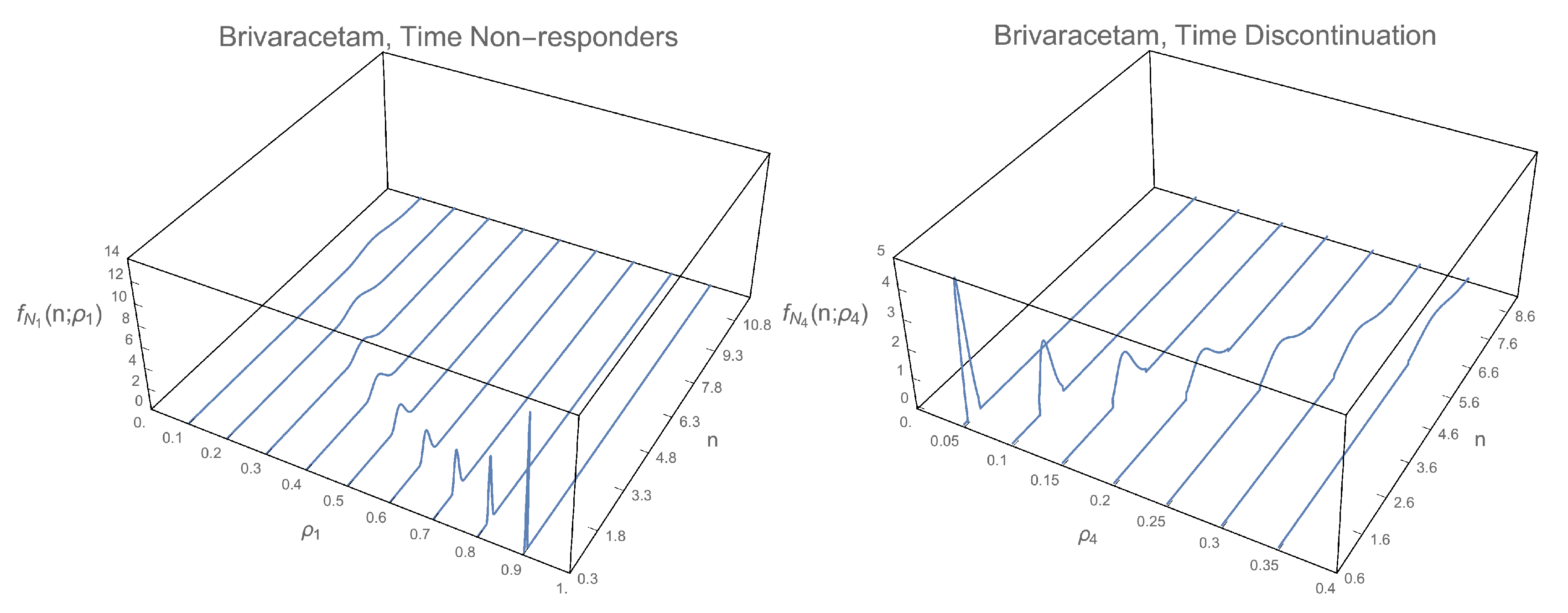
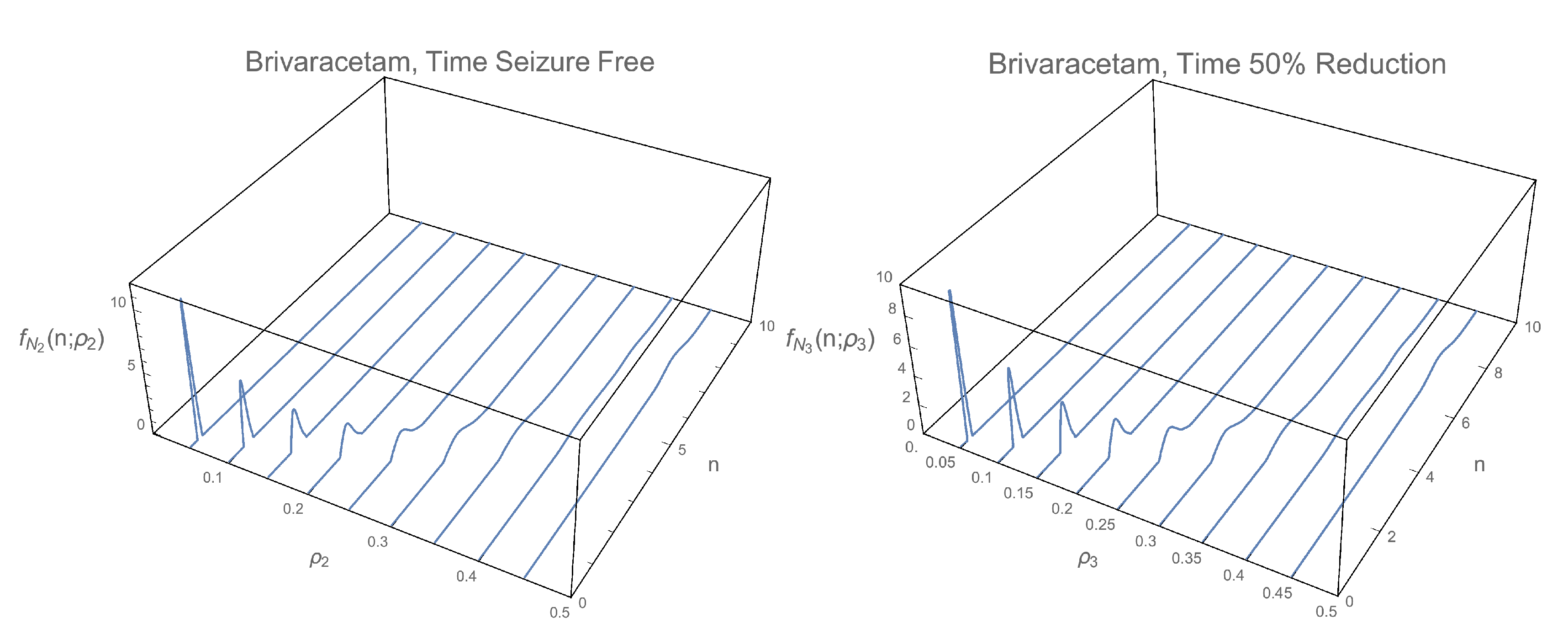
2.1. Computing the 1-PDF of $X_n$

In this subsection, we will apply RVT method, Theorem 1, to compute the 1-PDF of each stage $X_n^j$, with $j\in \{1,2,3,4\}$, considering that the joint PDF of random vector $\left(P_{12},P_{13},P_{14}\right)$, $f_{P_{12},P_{13},P_{14}}(p_{12},p_{13},p_{14})$, is known. Note that the procedure is analogous in each case. Therefore, to facilitate reading, the same structure is followed in any of them, clearly indicating the corresponding transformation.

2.1.1. 1-PDF of $X_n^1$

Firstly, we compute the 1-PDF of the proportion of non-responders $X_n^1={(1-P_{12}-P_{13}-P_{14})}^n$. Fixing the period $n>0$, we define the following mapping $\mathbf{r}:{\mathbb{R}}^3\to {\mathbb{R}}^3$

$$\begin{array}{c}{y}_1=r_1(p_{12},p_{13},p_{14})={(1-p_{12}-p_{13}-p_{14})}^n,\hfill \\ y_2=r_2(p_{12},p_{13},p_{14})=p_{13},\hfill \\ y_3=r_3(p_{12},p_{13},p_{14})=p_{14}.\hfill \end{array}$$

The inverse $\mathbf{s}:{\mathbb{R}}^3\to {\mathbb{R}}^3$ of the mapping $\mathbf{r}$ and the absolute value of its Jacobian are

$$\begin{array}{c}{p}_{12}=s_1(y_1,y_2,y_3)=1-y_1^{1/n}-y_2-y_3,\hfill \\ p_{13}=s_2(y_1,y_2,y_3)=y_2,\hfill \\ p_{14}=s_3(y_1,y_2,y_3)=y_3,\hfill \end{array}$$

and

$$\left|J\right|=\left|\frac{-y_1^{-1+1/n}}{n}\right|.$$

Thus, applying Theorem 1, the joint PDF of random vector $(Y_1,Y_2,Y_3)$ is

$$f_{Y_1,Y_2,Y_3}(y_1,y_2,y_3)=f_{P_{12},P_{13},P_{14}}\left(1-y_1^{1/n}-y_2-y_3,y_2,y_3\right)\left|\frac{-y_1^{-1+1/n}}{n}\right|.$$

The PDF of RV $Y_1=X_n^1$, n fixed, is obtained as the marginal PDF of $f_{Y_1,Y_2,Y_3}(y_1,y_2,y_3)$ with respect to $Y_2=P_{13}$ and $Y_3=P_{14}$

$$f_{Y_1}\left(y_1\right)={\int }_{{\mathbb{R}}^2}{f}_{P_{12},P_{13},P_{14}}\left(1-y_1^{1/n}-\delta -\eta ,\delta ,\eta \right)\left|\frac{-y_1^{-1+1/n}}{n}\right|\mathrm{d}\delta \mathrm{d}\eta .$$

Now, considering $n>0$ arbitrary, the 1-PDF of the solution SP $X_n^1=Y_1$ is given by

$$f_1^1(x;n)={\int }_{{\mathbb{R}}^2}{f}_{P_{12},P_{13},P_{14}}\left(1-x^{1/n}-\delta -\eta ,\delta ,\eta \right)\left|\frac{-x^{-1+1/n}}{n}\right|\mathrm{d}\delta \mathrm{d}\eta .$$

(7)

2.1.2. 1-PDF of $X_n^2$

To compute the 1-PDF of seizure free population $X_n^2=\frac{p_{12}({(1-p_{14})}^n-{(1-p_{12}-p_{13}-p_{14})}^n)}{p_{12}+p_{13}}$, given a fixed period $n>0$, we define the following mapping $\mathbf{r}:{\mathbb{R}}^3\to {\mathbb{R}}^3$,

$$\begin{array}{c}{\displaystyle y_1=r_1(p_{12},p_{13},p_{14})=\frac{p_{12}({(1-p_{14})}^n-{(1-p_{12}-p_{13}-p_{14})}^n)}{p_{12}+p_{13}},}\hfill \\ y_2=r_2(p_{12},p_{13},p_{14})=p_{12}+p_{13},\hfill \\ y_3=r_3(p_{12},p_{13},p_{14})=1-p_{14}.\hfill \end{array}$$

The inverse $\mathbf{s}:{\mathbb{R}}^3\to {\mathbb{R}}^3$ of the mapping $\mathbf{r}$ and the absolute value of its Jacobian is

$$\begin{array}{c}{\displaystyle p_{12}=s_1(y_1,y_2,y_3)=\frac{y_1{y}_2}{y_3^n-{(y_3-y_2)}^n},}\hfill \\ {\displaystyle p_{13}=s_2(y_1,y_2,y_3)=y_2\left(1-\frac{y_1}{y_3^n-{(y_3-y_2)}^n}\right),}\hfill \\ {\displaystyle p_{14}=s_3(y_1,y_2,y_3)=1-y_3,}\hfill \end{array}$$

and

$$\left|J\right|=\left|\frac{y_2}{y_3^n-{(y_3-y_2)}^n}\right|.$$

Therefore, according to Theorem 1, the joint PDF of random vector $(Y_1,Y_2,Y_3)$ is

$$f_{Y_1,Y_2,Y_3}(y_1,y_2,y_3)=f_{P_{12},P_{13},P_{14}}\left(\frac{y_1{y}_2}{y_3^n-{(y_3-y_2)}^n},y_2\left(1-\frac{y_1}{y_3^n-{(y_3-y_2)}^n}\right),1-y_3\right)\left|\frac{y_2}{y_3^n-{(y_3-y_2)}^n}\right|.$$

The PDF of RV $Y_1=X_n^2$, n fixed, is obtained marginalizing the PDF of $f_{Y_1,Y_2,Y_3}(y_1,y_2,y_3)$ with respect to $Y_2$ and $Y_3$

$$f_{Y_1}\left(y_1\right)={\int }_{{\mathbb{R}}^2}{f}_{P_{12},P_{13},P_{14}}\left(\frac{y_1\delta }{{\eta }^n-{(\eta -\delta )}^n},\delta \left(1-\frac{y_1}{{\eta }^n-{(\eta -\delta )}^n}\right),1-\eta \right)\left|\frac{\delta }{{\eta }^n-{(\eta -\delta )}^n}\right|\mathrm{d}\delta \mathrm{d}\eta .$$

Now, considering $n>0$ arbitrary, the 1-PDF of the solution SP $X_n^2=Y_1$ is given by

$$f_1^2(x;n)={\int }_{{\mathbb{R}}^2}{f}_{P_{12},P_{13},P_{14}}\left(\frac{x\delta }{{\eta }^n-{(\eta -\delta )}^n},\delta \left(1-\frac{x}{{\eta }^n-{(\eta -\delta )}^n}\right),1-\eta \right)\left|\frac{\delta }{{\eta }^n-{(\eta -\delta )}^n}\right|\mathrm{d}\delta \mathrm{d}\eta .$$

(8)

2.1.3. 1-PDF of $X_n^3$

Analogous to the previous case, the 1-PDF of partial responders $X_n^3=\frac{P_{13}({(1-P_{14})}^n-{(1-P_{12}-P_{13}-P_{14})}^n)}{P_{12}+P_{13}}$ is obtained considering a similar transformation

$$f_1^3(x;n)={\int }_{{\mathbb{R}}^2}{f}_{P_{12},P_{13},P_{14}}\left(\delta \left(1-\frac{x}{{\eta }^n-{(\eta -\delta )}^n}\right),\frac{x\delta }{{\eta }^n-{(\eta -\delta )}^n},1-\eta \right)\left|\frac{-\delta }{{\eta }^n-{(\eta -\delta )}^n}\right|\mathrm{d}\delta \mathrm{d}\eta .$$

(9)

2.1.4. 1-PDF of $X_n^4$

To conclude section, we obtain the 1-PDF of population with drug discontinuation symptoms $X_n^4=\left(1-{\left(1-p_{14}\right)}^n\right)$. Fixed $n>0$, we define the mapping $r:\mathbb{R}\to \mathbb{R}$ as

$$y=r\left(p_{14}\right)=1-{(1-p_{14})}^n.$$

The inverse $s:\mathbb{R}\to \mathbb{R}$ of the mapping r, and the absolute value of its Jacobian is

$$p_{14}=s\left(y\right)=1-{\left(1-y\right)}^{1/n}\mathrm{and}\left|J\right|=\left|\frac{{(1-y)}^{-1+1/n}}{n}\right|.$$

Applying RVT method, Theorem 1, the PDF of RV Y is

$$f_Y\left(y\right)=f_{P_{14}}\left(1-{\left(1-y\right)}^{1/n}\right)\left|\frac{{(1-y)}^{-1+1/n}}{n}\right|.$$

Now, considering $n>0$ arbitrary, the 1-PDF of the solution SP $X_n^4=Y$ is given by

$$f_1^4(x;n)=f_{P_{14}}\left(1-{\left(1-x\right)}^{1/n}\right)\left|\frac{{(1-x)}^{-1+1/n}}{n}\right|.$$

(10)

Notice that, by hypothesis, we know the joint distribution of random vector $(P_{12},P_{13},P_{14})$. From it, the PDF of RV $P_{14}$ can be easily calculated, marginalizing the joint PDF with regard to the other two RVs $P_{12}$ and $P_{13}$

$$f_{P_{14}}\left(p\right)={\int }_{{\mathbb{R}}^2}{f}_{P_{12},P_{13},P_{14}}(\delta ,\eta ,p)\mathrm{d}\delta \mathrm{d}\eta .$$

2.2. Computing the Pdf of the Time

We have determined the distribution of the number of individuals in each stage described in the Introduction, Section 1. From an applied point of view, it is advantageous to know when the proportion of persons in each stage attain a specific level. Let $N_j$ be the time until a given proportion of the population, ${\rho }_j$, remains in the stage $j\in \{1,2,3,4\}$, ${\rho }_j=X_{N_j}^j$. Here below, the PDF of $N_1$ and $N_4$ are computed. Notice that, distributions $N_2$ and $N_3$ are not determined applying RVT method since n cannot be easily isolated in

$${\rho }_i=\frac{p_{1i}({(1-p_{14})}^n-{(1-p_{12}-p_{13}-p_{14})}^n)}{p_{12}+p_{13}},i\in \{2,3\}.$$

Then, in these cases we have not an explicit expression for the time. In Section 3, we apply numerical methods to compute the probability distributions of $N_2$ and $N_3$. In particular, we use Newton-Raphson method, to calculate the roots of the non-linear equation previously indicated. The methodology is explained in detail in the numerical example, Section 3.

2.2.1. PDF of $N_1$

Let ${\rho }_1$ be a given non-responder population. If we consider $n=N_1$ an absolutely continuous RV, from expression (6), the exact solution is

$${\rho }_1={\left(1-P_{12}-P_{13}-P_{14}\right)}^{N_1}.$$

Isolating from that expression $N_1$

$$N_1=\frac{log\left({\rho }_1\right)}{log(1-P_{12}-P_{13}-P_{14})}.$$

Notice that $N_1$ is well defined since ${\rho }_1$ is a constant, which represent the proportion of non-responder population, i.e., is a fixed number between 0 and 1. Moreover, $1-P_{12}-P_{13}-P_{14}$ represents the probability of remains non-responder, therefore it also lies between 0 and 1. In addition, as $P_{12}$, $P_{13}$ and $P_{14}$ are continuous RVs then

$$\mathbb{P}\left[\omega \in \mathsf{\Omega }:1-P_{12}\left(\omega \right)-P_{13}\left(\omega \right)-P_{14}\left(\omega \right)=0\right]=0=\mathbb{P}\left[\omega \in \mathsf{\Omega }:1-P_{12}\left(\omega \right)-P_{13}\left(\omega \right)-P_{14}\left(\omega \right)=1\right].$$

Now, we apply Theorem 1 to the following transformation $\mathbf{r}:{\mathbb{R}}^3\to {\mathbb{R}}^3$

$$\begin{array}{c}{y}_1=r_1(p_{12},p_{13},p_{14})=\frac{log\left({\rho }_1\right)}{log(1-p_{12}-p_{13}-p_{14})},\hfill \\ y_2=r_2(p_{12},p_{13},p_{14})=p_{13},\hfill \\ y_3=r_3(p_{12},p_{13},p_{14})=p_{14}.\hfill \end{array}$$

The inverse $\mathbf{s}:{\mathbb{R}}^3\to {\mathbb{R}}^3$ of the mapping $\mathbf{r}$ and the absolute value of its Jacobian is

$$\begin{array}{c}{p}_{12}=s_1(y_1,y_2,y_3)=1-y_2-y_3-{\rho }_1^{1/y_1},\hfill \\ p_{13}=s_2(y_1,y_2,y_3)=y_2,\hfill \\ p_{14}=s_3(y_1,y_2,y_3)=y_3,\hfill \end{array}$$

and

$$\left|J\right|=\left|\frac{{\rho }_1^{1/y_1}log\left({\rho }_1\right)}{y_1^2}\right|.$$

Therefore, according to Theorem 1, the joint PDF of random vector $(Y_1,Y_2,Y_3)$ is

$$f_{Y_1,Y_2,Y_3}(y_1,y_2,y_3)=f_{P_{12},P_{13},P_{14}}\left(1-y_2-y_3-{\rho }_1^{1/y_1},y_2,y_3\right)\left|\frac{{\rho }_1^{1/y_1}log\left({\rho }_1\right)}{y_1^2}\right|.$$

The PDF of RV $Y_1=N_1$, is determined by marginalizing $f_{Y_1,Y_2,Y_3}(y_1,y_2,y_3)$ with respect to $(Y_2,Y_3)=(P_{13},P_{14})$

$$f_{N_1}(n;{\rho }_1)={\int }_{{\mathbb{R}}^2}{f}_{P_{12},P_{13},P_{14}}\left(1-\delta -\eta -{\rho }_1^{1/n},\delta ,\eta \right)\left|\frac{{\rho }_1^{1/n}log\left({\rho }_1\right)}{n^2}\right|\mathrm{d}\delta \mathrm{d}\eta .$$

(11)

2.2.2. PDF of $N_4$

To finish this subsection, we obtain the PDF of the RV $N_4$, this is, the time until a given proportion of the population with discontinuation symptoms, ${\rho }_4$, remains in the same stage,

$$N_4=\frac{log(1-{\rho }_4)}{log(1-P_{14})}.$$

Notice that, this formula is well defined since $\mathbb{P}[1-P_{14}\left(\omega \right)\le 0]=0$. In this case, we apply RVT method, Theorem 1, considering

$$n=r\left(p_{14}\right)=\frac{log(1-{\rho }_4)}{log(1-p_{14})},p_{14}=s\left(n\right)=1-{(1-{\rho }_4)}^{1/n},\mathrm{and}\left|J\right|=\left|\frac{{(1-{\rho }_4)}^{1/n}log(1-{\rho }_4)}{n^2}\right|.$$

Therefore, the PDF of RV $T=N_4$ is

$$f_{N_4}(n;{\rho }_4)=f_{P_{14}}\left(1-{(1-{\rho }_4)}^{1/n}\right)\left|\frac{{(1-{\rho }_4)}^{1/n}log(1-{\rho }_4)}{n^2}\right|.$$

Now, as previously, the PDF of the RV $P_{14}$ can be calculated from the joint PDF of the random vector $(P_{12},P_{13},P_{14})$

$$f_{P_{14}}\left(p\right)={\int }_{{\mathbb{R}}^2}{f}_{P_{12},P_{13},P_{14}}(\delta ,\eta ,p)\mathrm{d}\delta \mathrm{d}\eta .$$

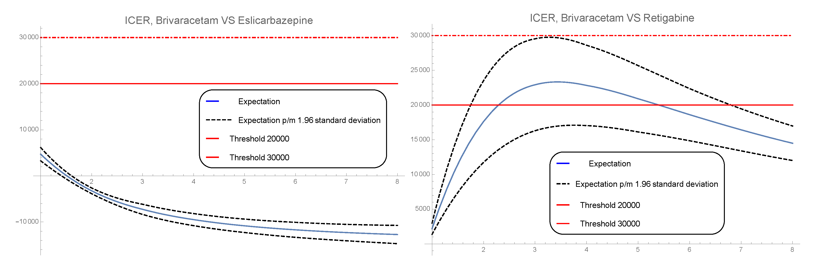
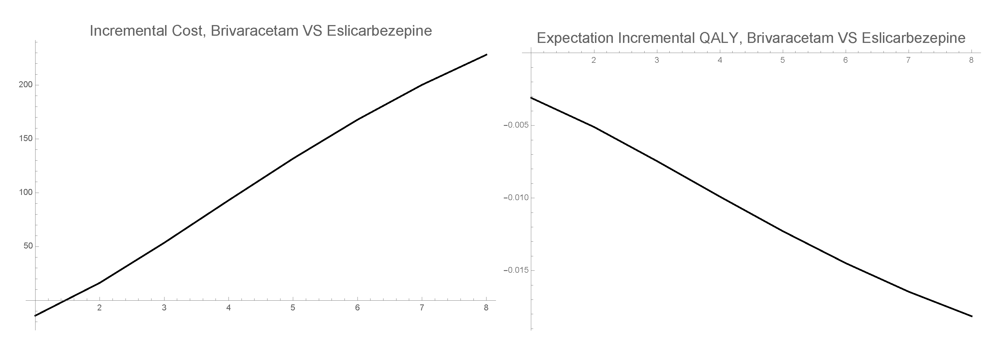
2.3. Computing the Approximated Pdf of the Incremental Cost-Effectiveness Ratio (Icer)

As it was pointed before, the main objective of AEDs is to improve the quality of life of patients. However, all AEDs cause uncomfortable adverse effects, which influence the quality of life outcomes of the patients, such as nausea, with a certain probability. We consider five adverse events, each one with an associated probability: Ataxia, $P_A$; Dizziness, $P_D$; Fatigue, $P_F$; Nausea, $P_N$; Somnolence, $P_S$. In this subsection, we obtain the 1-PDF of the ICER taking into account that the probabilities previously introduced, $P_A,P_D,P_F,P_N$ and $P_S$ are dependent absolutely continuous RVs with a known PDF. ICER is convenient to compare two different treatments taking into account the total cost and the quality of life of the patient. That is, a cost-effectiveness analysis is useful to prioritize sanitary interventions taking into account available resources [19,20]. The ICER is the ratio of the increment of cost over the increment of effectiveness between two treatments

$$\mathrm{ICER}=\frac{c_2-c_1}{E_2-E_1},$$

(12)

where $c_i$ and $E_i$ are the total cost and the effectiveness of the alternative $i\in \{1,2\}$, respectively. In the following, we treat with two treatments, that is, we have two populations, X and Y, and in each population four states. In addition, the treatment is studied in n cycles. Therefore, respect with the population we have $8n$ RVs. To these RVs we must add the ones corresponding to the adverse effects in each population. Then, we deal in total with $8n+10$ RVs. Computationally, this is infeasible, thus we are going to compute approximations of the PDF of the ICER. These approximations are calculated considering in the following the expectation of each $X_j^i$ and $Y_j^i$ for $j\in 1,\dots ,n$ and $i\in 1,2,3,4$, $\mathbb{E}\left[X_j^i\right]$ and $\mathbb{E}\left[Y_j^i\right]$. As we know the PDF of each RV, see Section 2.2, this expectation can be easily computed. In this manner, we will finally work with 10 RVs.

Now, we shall define the cost and the effectiveness in Formula (12). The effectiveness of each treatment is the so-called QALY, and it is the sum of the effectiveness at each stage. In addition, the effectiveness of each of the four stages is the sum of the effectiveness in each period until the value n of the total of quarters considered. Furthermore, the effectiveness can be defined as the product of the corresponding number of patients by the utility. Then, we define the effectiveness per cycle as

$$E=0.25\sum _{j=1}^n\left(\sum _{i=1}^4{u}_j^i+U_j^{*}\right),$$

(13)

where we multiply by 0.25 since normally the utilities are given per year and we consider 3 month periods. In expression (13) $U_j^{*}$ denotes the total QALY reduction given by adverse events

$$U_j^{*}=U_{j,A}+U_{j,D}+U_{j,F}+U_{j,N}+U_{j,S},$$

being, for example for the Ataxia event $U_{j,A}=\left(\mathbb{E}\left[X_{j-1}^2\right]+\mathbb{E}\left[X_{j-1}^3\right]\right)P_A{u}_A$, $j\ge 2$, and $P_A{u}_A$ with $j=1$, being $u_A\le 0$ the utility reduction of the Ataxia. On the other hand, $u_j^i$ is considered a deterministic value, and it represents the utility in each period j for each stage i: $u_j^i=\mathbb{E}\left[X_j^i\right]u_i$, where $u_i$ is the utility in each stage $i\in \{1,2,3,4\}$. Now, we define the cost function as the sum of the costs in each stage for each period

$$c=\sum _{j=1}^n\left(\sum _{i=1}^4\mathbb{E}\left[X_j^i\right]\left(\left(c_D+c_A\right)90+c^i\right)\right)-\sum _{j=2}^n\mathbb{E}\left[X_{j-1}^4\right]c_{D}90+c_T-d_{NE}{C}_D,$$

or, applying the Markovian property, ${\sum }_{i=1}^4{X}_j^i=1$, equivalently

$$c=n\left(c_D+c_A\right)90+\sum _{j=1}^n\left(\sum _{i=1}^4\mathbb{E}\left[X_j^i\right]c^i\right)-90c_D\sum _{j=2}^n\mathbb{E}\left[X_{j-1}^4\right]+c_T-d_{NE}{C}_D,$$

(14)

where $c_D$, $c_A$ and $c_T$ are treatment costs defined as

• $c_D$ is the daily AEDs cost.
• $c_A$ is the average cost of concomitant Monotherapy.
• $c_T$ is the Titration total cost.

In addition, $c^i$ denotes the quarterly cost service utilization, including the cost of inpatient care, emergency visit, an outpatient visit to the neurologist, etc. The value $c^i$ depend on the number of crisis of the patient. Notice that $c_D$ and $c_A$ are multiplied by 90, since both values are given per day, and we work in three month periods (3 months = 90 days). In expression (14), the value $d_{NE}$ corresponds with the total days until the patient is within a therapeutic dosage range.

Let $X_j$ and $Y_j$ be the solutions SPs of people subjected to first and second treatments, respectively. Therefore, ICER can be obtained from Formulas (12)–(14) taking into account these two different treatments

$$\mathrm{ICER}=\frac{k}{q+q_1\left(P_{A,1}{u}_A+P_{D,1}{u}_D+P_{F,1}{u}_F+P_{N,1}{u}_N+P_{S,1}{u}_S\right)-q_2\left(P_{A,2}{u}_A+P_{D,2}{u}_D+P_{F,2}{u}_F+P_{N,2}{u}_N+P_{S,2}{u}_S\right)},$$

(15)

being, for example, $P_{A,i}$ the probability of Ataxia with the treatment i and the values k, $q_1$ and $q_2$ deterministic constants that can be obtained from the cost and the effectiveness previously defined

$$\begin{array}{cc}k=c_X-c_Y,\hfill & {\displaystyle q=0.25\sum _{j=1}^n\sum _{i=1}^4\left(\mathbb{E}\left[X_j^i\right]-\mathbb{E}\left[Y_j^i\right]\right)u_i,}\hfill \\ {\displaystyle q_1=0.25\left(1+\sum _{j=2}^n\left(\mathbb{E}\left[X_{j-1}^2\right]+\mathbb{E}\left[X_{j-1}^3\right]\right)\right),}\hfill & {\displaystyle q_2=0.25\left(1+\sum _{j=2}^n\left(\mathbb{E}\left[Y_{j-1}^2\right]+\mathbb{E}\left[Y_{j-1}^3\right]\right)\right),}\hfill \end{array}$$

where $c_X$ and $c_Y$ are the cost of treatment for population X and Y, respectively.

In the following, to simplify the notation, we consider only two adverse effects, Ataxia and Dizziness. The same argument can be followed with the five events previously introduced as well as if another one needs to be considered. Now, RVT technique, Theorem 1, is applied to compute the 1-PDF of the ICER. Let $n>0$ fixed, we define the mapping $\mathbf{r}:{\mathbb{R}}^4\to {\mathbb{R}}^4$,

$$\begin{array}{c}{\displaystyle y_1=r_1(p_{A,1},p_{A,2},p_{D,1},p_{D,2})=\frac{k}{q+q_1\left(p_{A,1}{u}_A+p_{D,1}{u}_D\right)-q_2\left(p_{A,2}{u}_A+p_{D,2}{u}_D\right)},}\hfill \\ {\displaystyle y_2=r_2(p_{A,1},p_{A,2},p_{D,1},p_{D,2})=p_{A,2},}\hfill \\ y_3=r_3(p_{A,1},p_{A,2},p_{D,1},p_{D,2})=p_{D,1},\hfill \\ y_4=r_4(p_{A,1},p_{A,2},p_{D,1},p_{D,2})=p_{D,2},\hfill \end{array}$$

The inverse $\mathbf{s}:{\mathbb{R}}^4\to {\mathbb{R}}^4$ of the mapping $\mathbf{r}$ and the absolute value of its Jacobian are

$$\begin{array}{c}{\displaystyle p_{A,1}=s_1(y_1,y_2,y_3,y_4)=\left(\left(\frac{k}{y_1}-q+q_2(y_2{u}_A+y_4{u}_D)\right)\frac{1}{q_1}-y_3{u}_D\right)\frac{1}{u_A},}\hfill \\ {\displaystyle p_{A,2}=s_2(y_1,y_2,y_3,y_4)=y_2,}\hfill \\ {\displaystyle p_{D,1}=s_3(y_1,y_2,y_3,y_4)=y_3,}\hfill \\ {\displaystyle p_{D,2}=s_3(y_1,y_2,y_3,y_4)=y_4.}\hfill \end{array}$$

and

$$\left|J\right|=\left|\frac{-k}{u_A{q}_1{y}_1^2}\right|.$$

Therefore, according to Theorem 1, and taking n arbitrary the 1-PDF of the ICER is

$$f_1^{\mathrm{ICER}}(x;n)={\int }_{{\mathbb{R}}^3}{f}_{AE}\left(\left(\left(\frac{k}{x}-q+q_2(\eta u_A+\mu u_D)\right)\frac{1}{q_1}-\delta u_D\right)\frac{1}{u_A},\eta ,\delta ,\mu \right)\left|\frac{-k}{u_A{q}_1{x}^2}\right|\mathrm{d}\eta \mathrm{d}\delta \mathrm{d}\mu ,$$

(16)

being $f_{A}E$ the PDF of the random vector $(P_{A,1},P_{A,2},P_{D,1},P_{D,2})$.

3. Numerical Example

In this section, we show the capability of the theoretical findings previously established, which have been obtained applying the RVT method. We divide the numerical simulations using real data into three parts, as in the theory, 1-PDF of the solution SP, PDF of the time and 1-PDF of the ICER. As it has been pointed at the introduction Brivaracetam is a new third-generation AED, then it is interesting to analyse, from a probabilistic point of view this treatment. As indicated in the introduction, the main advantages of this medicine are its fixed cost, independent of dose, and it does not need tritation.

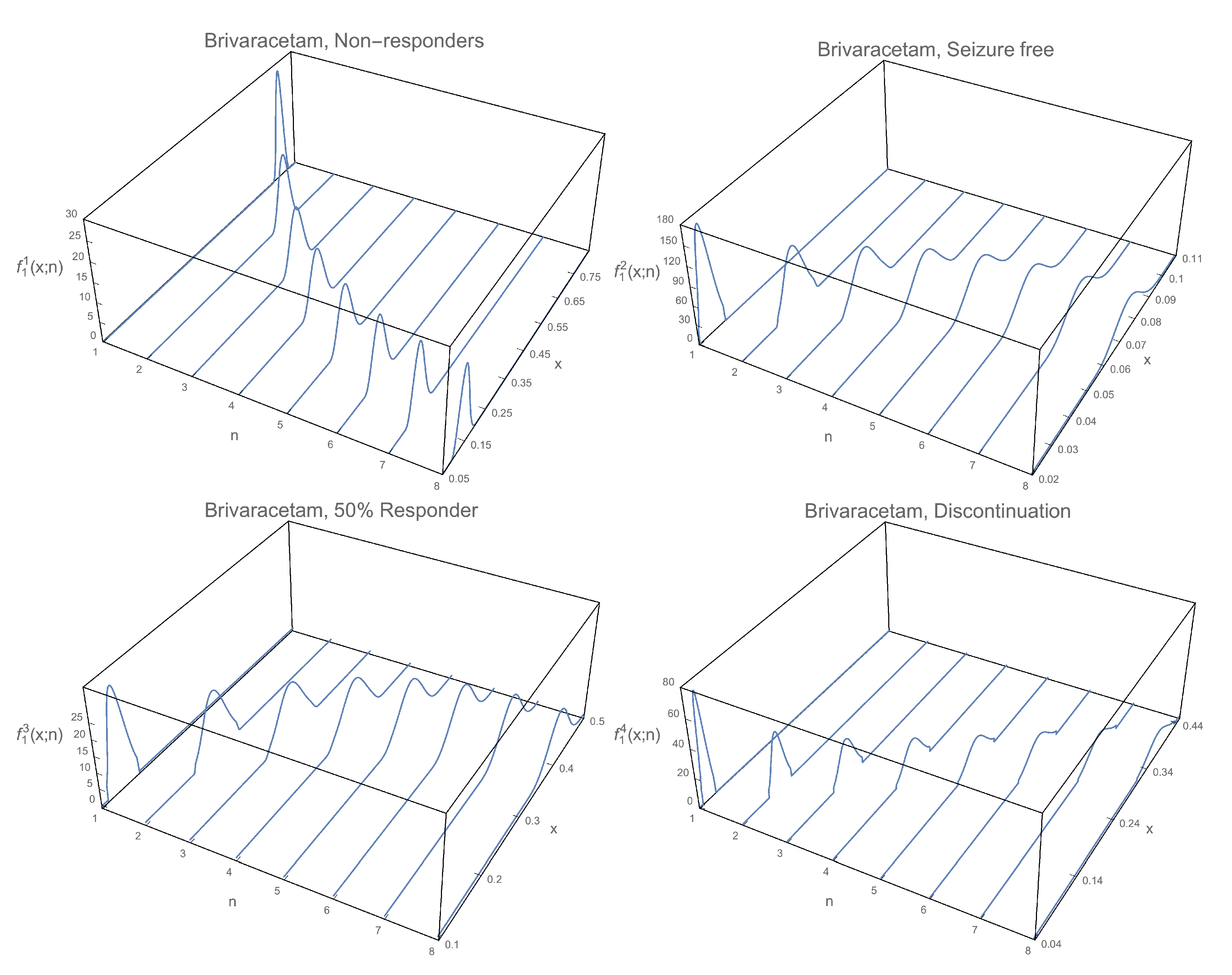
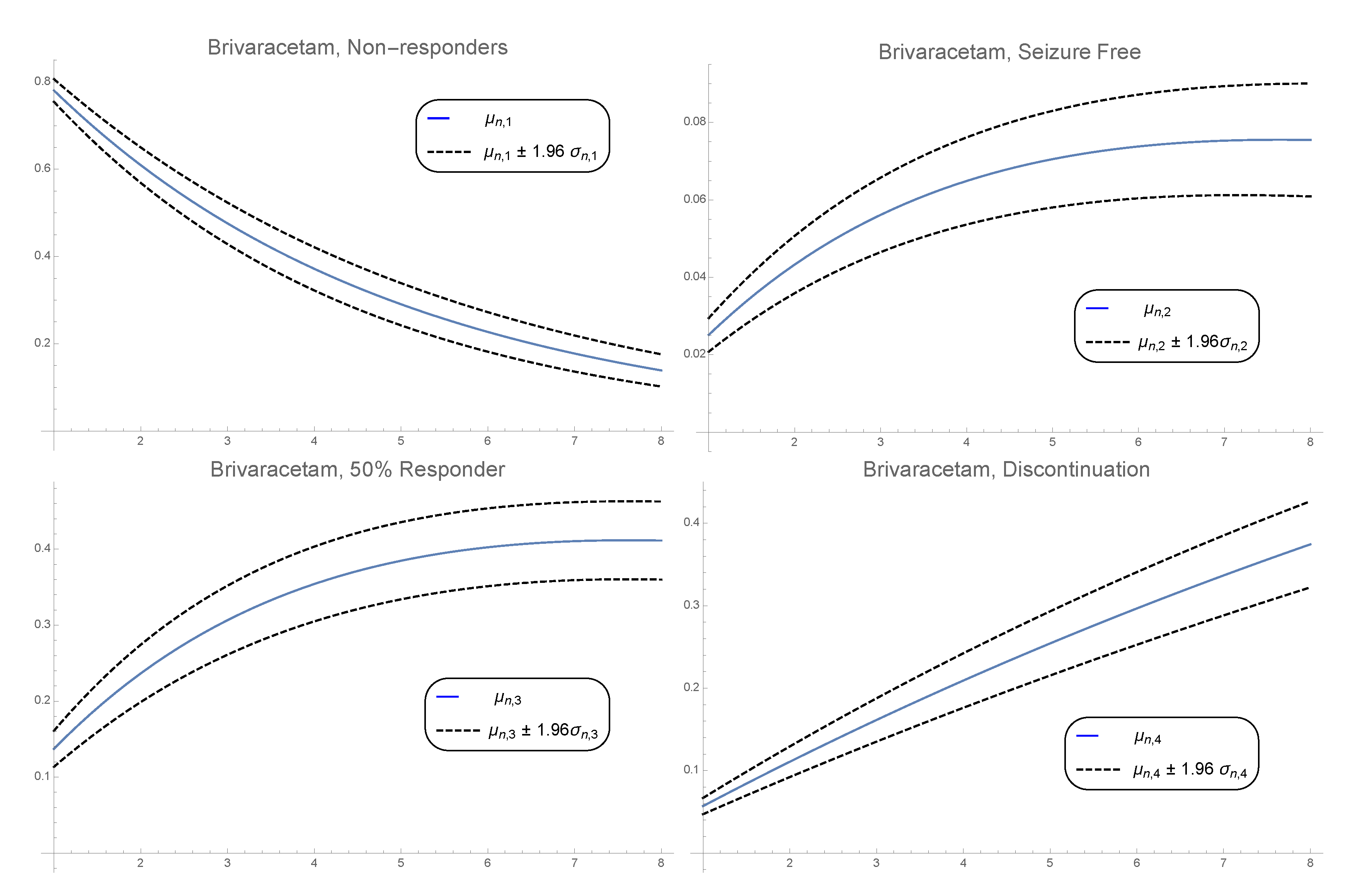
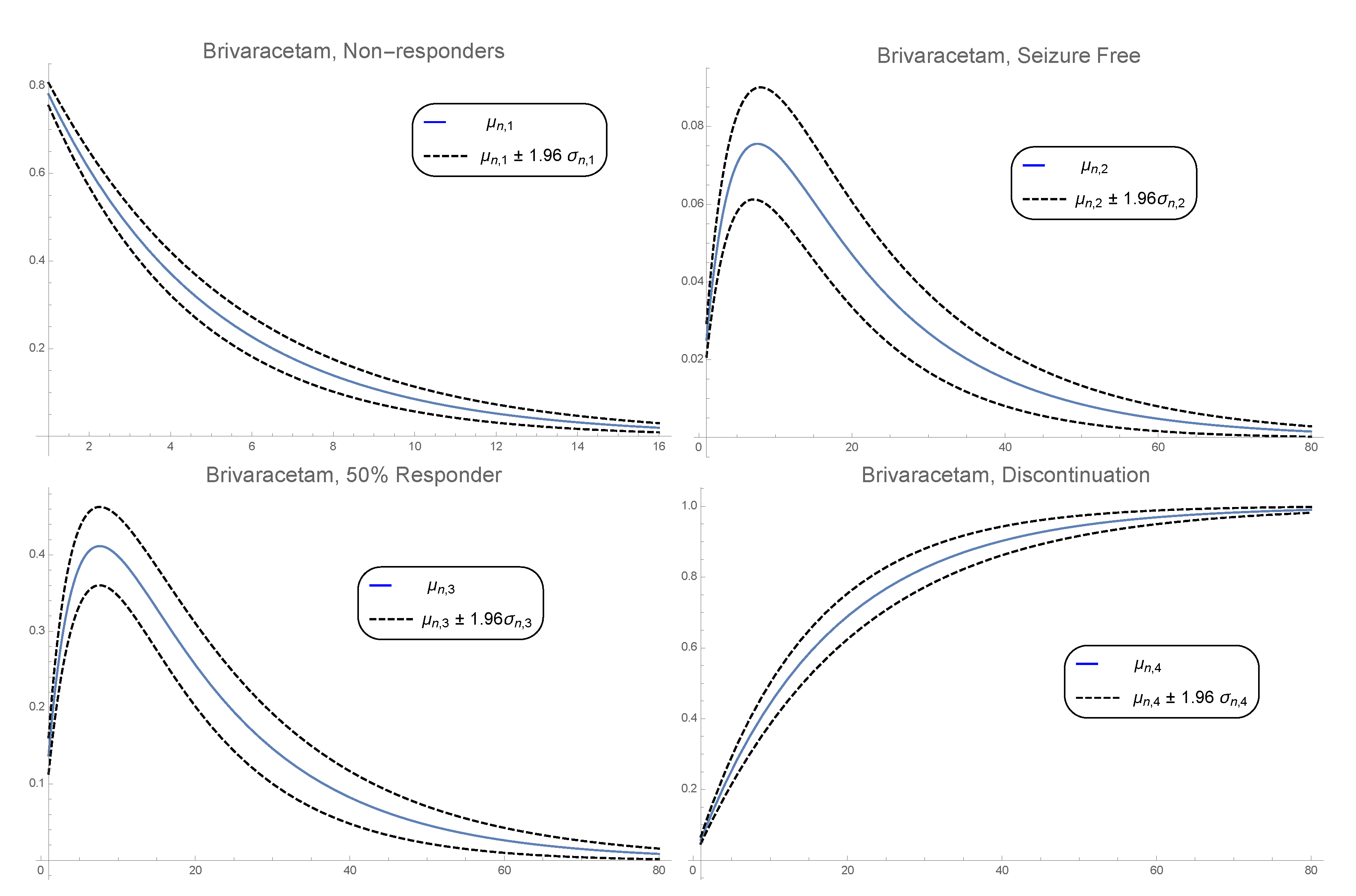
3.1. 1-Pdf of the Solution Sp

The probabilities of transition between health states have been obtained from a Network meta-analysis, which is a methodology that synthesise networks of direct and indirect comparisons of interventions, and facilitate researchers to simultaneously check the effects of more than two interventions for the same condition [21]. These probabilities are calculated for one year of treatment, the following matrix for the Brivaracetam AED is obtained [15]

$$\left(\begin{array}{cccc}0.37& 0& 0& 0\\ 0.065& 0.79& 0& 0\\ 0.355& 0& 0.79& 0\\ 0.21& 0.21& 0.21& 1\end{array}\right).$$

For a three month period the corresponding matrix can be calculated [15,22]

$${\left(\begin{array}{cccc}0.37& 0& 0& 0\\ 0.065& 0.79& 0& 0\\ 0.355& 0& 0.79& 0\\ 0.21& 0.21& 0.21& 1\end{array}\right)}^{1/4}=\left(\begin{array}{cccc}0.7799& 0& 0& 0\\ 0.0252& 0.9428& 0& 0\\ 0.1376& 0& 0.9428& 0\\ 0.0572& 0.0572& 0.0572& 1\end{array}\right)$$

Then, for Brivaracetam AED $p_{12}=0.02520$, $p_{13}=0.13765$ and $p_{14}=0.0572$. Now, we assume that $P_{12}$, $P_{13}$ and $P_{14}$ are independent absolutely continuous RVs. In order to establish the PDFs of each RV we consider that the corresponding deterministic values are perturbed. Then, we choose for each RV, a Beta distribution $P_{1i}\sim \mathrm{Be}(a_i;b_i)$, $i\in \{2,3,4\}$ with

$$a_i={\mu }_i\left(\frac{{\mu }_i(1-{\mu }_i)}{{\sigma }_i^2}-1\right),b_i=(1-{\mu }_i)\left(\frac{{\mu }_i(1-{\mu }_i)}{{\sigma }_i^2}-1\right),$$

where both quantities are obtained from the definition of mean and variance of a Beta distribution, $X\sim \mathrm{Be}(a;b)$, isolating the parameters a and b from

$$\mathbb{E}\left[X\right]=\mu =\frac{a}{a+b},\mathbb{V}\left[X\right]={\sigma }^2=\frac{ab}{{(a+b)}^2(a+b+1)}.$$

Finally, we take as the mean the deterministic value ${\mu }_i=p_{1,i}$, and the variance ${\sigma }_i=0.1{\mu }_i$, small enough since it represents the dispersion or variability, for each $i\in \{2,3,4\}$. With this selection of distributions it can be proven that

$$\mathbb{P}\left[\omega \in \mathsf{\Omega },0\le P_{1,2}\left(\omega \right)+P_{1,3}\left(\omega \right)+P_{1,4}\left(\omega \right)\le 1\right]=1$$

In Figure 2, the 1-PDFs of each state described in Figure 1 have been plotted. These graphical representations have been made for periods $n\in \{1,2,\dots ,8\}$, that is, we study what happen in two years. In Figure 3, we show the mean plus/minus 1.96 standard deviation functions corresponding to each subpopulation. Observe that, both graphical representations, Figure 2 and Figure 3, agree. Non-responder population decreases with the time, while patients with discontinuation symptoms increase over the time. With respect to the other two states, both increase for the first periods, and then, then decreases. This fact is more evident in Figure 4. In model (1) we observe that the discontinuation state is an absorbent state. We cannot observe properly, this circumstance in Figure 2 and Figure 3 since we take into account few periods, 8 in total. Thus, to show this fact in Figure 4 we plot the mean plus/minus 1.96 standard deviation for all subpopulations, considering greater times. In Figure 4 we observe that the proportion of subpopulation with discontinuation increases tending towards one, while the other subpopulations vanish as time goes on, in agreement with the absorbent character of patients with discontinuation symptoms. We highlight that the 1-PDF is very useful since, from its expression, we are able to obtain exact confidence intervals in order to perform reliable probabilistic predictions. In addition, it allows us to compute probabilities associated to sets of interest. For example, one can calculate the probability that the proportion of non-responders lies between $0.35$ and $0.45$ in the time period $\widehat{n}=4$

$$\mathbb{P}\left[0.35\le X_4^1\le 0.45\right]={\int }_{0.35}^{0.45}{f}_1^1(x,4)\mathrm{d}x=0.792045.$$

3.2. Pdf of the Time

Now, we calculate the PDFs of time until a fixed proportion of the population remains in each of the states described in Figure 1. As it was pointed in Section 2.2 the exact expression of these functions have been determined in the cases of non-responders and patients with discontinuation symptoms. In Figure 5 both PDFs are shown for different values of ${\rho }_1\in \{0.1,0.2,\dots ,0.9\}$ and ${\rho }_4\in \{0.05,0.1,\dots ,0.35\}$. As before, from the PDF we can compute the mean for a fixed proportion. For example, for non-responders, the expectation of RV $N_1$ for ${\rho }_1=0.6$ is computed as follows,

$$\mathbb{E}\left[N_1\right]={\int }_0^{\infty }n{f}_{N_1}(n;0.6)=2.07022.$$

Then, approximately a semester ($n=4$ correspond to a year), represents the average time until $60\%$ of population will be non-responder.

Table 1. Expectation of time until a given proportion of population, ${\rho }_1$, remains non-responder, $N_1$.

${\mathit{\rho }}_1$	$0.1$	$0.2$	$0.3$	$0.4$	$0.5$	$0.6$	$0.7$	$0.8$	$0.9$
$\mathbb{E}\left[N_1\right]$	$9.33167$	$6.52255$	$4.87933$	$3.71344$	$2.80911$	$2.07022$	$1.44549$	$0.904332$	$0.426994$

collects this expectation for different values of ${\rho }_1$.

In order to obtain the PDFs of RVs $N_2$ and $N_3$, given fixed proportions ${\rho }_2$ and ${\rho }_3$, we have applied numerical methods. Below we indicate the steps corresponding to partial responders, $N_3$, assuming ${\rho }_3$ fixed:

• Step 1: To sample 500,000 values of the form $(p_{12},p_{13},p_{14})$, according with the distributions assumed for RVs $P_{12}$, $P_{13}$ and $P_{14}$.
• Step 2: For each sample in Step 1 we solve the non-linear equation

  $${\rho }_3=\frac{p_{13}({(1-p_{14})}^n-{(1-p_{12}-p_{13}-p_{14})}^n)}{p_{12}+p_{13}},$$

  to calculate the values n of $N_3$, using Newton-Raphson method. From these values, in the subsequent development, the minimum n is selected.
• Step 3: To plot the histogram with the 500,000 values of n. An approximation of the PDF of $N_3$ is obtained by normalizing this histogram.

In Figure 6 the PDFs of $N_2$ and $N_3$, constructed following this methodology, have been represented.

3.3. 1-PDF of ICER

Finally, we compute the 1-PDF of the ICER, which has been determined in Section 2.3 and given by Formula (16) but considering the five adverse effects. We compare Brivaracetam with other treatments: Eslicarbazepine and Retigabine, which are third-generation AEDs. All of them approved by the US Food & Drug Administration and the European Medicines Agency in January 2016 [9]. The eslicarbazepine was recently authorized also in children and adolescents as adjunctive treatment. Notice that, Retigabine has recently been withdrawn from the market due to the adverse effects it caused.

First of all, we must define all the quantities involved in the cost-effectiveness analysis. As indicated previously, the probabilities of transition between health states have been obtained from a Network meta-analysis [21]. The utilities and the probabilities of presenting adverse effects work as dis-benefits, which influence the quality of life outcomes of the patient, were taken from the Mulhern et al study of the quarterly cycles of the model, see [23]. The source for estimating the costs of each AED was the Spanish Ministry of Health [24] and BOT-PLUS [25]. Ex-factory prices were taken. With the exception of Brivaracetan, the rest of the medicines in the model required the estimation of the specific titration costs for each pharmacy [26]. In both AEDs, Eslicarbazepine and Retigabien this time period is established in two weeks. Then, $d_{NE}=0$ for Brivaracetam while for the other two treatments this quantity takes the value 14.

• Probabilities of response, partial response and discontinuation [21]. Brivaracetam: $p_{12}=0.02520$, $p_{13}=0.13765$, $p_{14}=0.0572$. Eslicarbazepine: $p_{12}=0.0112$, $p_{13}=0.1160$, $p_{14}=0.0452$. Retigabine: $p_{12}=0.0122$, $p_{13}=0.1577$, $p_{14}=0.0763$. These quantities will be used to calculate the different expectation in the cost and the effectiveness formulas, $\mathbb{E}\left[X_j^i\right]$, where $X_j^i$ is the solution SP in cycle j of the state i given in Formula (6).
• Probabilities of adverse events, Ataxia, Dizziness, Fatigue, Nausea and Somnolence [23] As previously, these probabilities will be considered independent absolutely continuous RVs. We choose for each RV a Beta distribution with parameters a and b calculated as before considering the following mean $\mu$. Brivaracetam: ${\mu }_A=0.00747$, ${\mu }_D=0.03198$, ${\mu }_F=0.02717$, ${\mu }_N=0.01242$, ${\mu }_S=0.03439$. Eslicarbazepine: ${\mu }_A=0.01489$, ${\mu }_D=0.05588$, ${\mu }_F=0.01489$, ${\mu }_N=0.02955$, ${\mu }_S=0.02955$. Retigabine: ${\mu }_A=0.01242$, ${\mu }_D=0.06059$, ${\mu }_F=0.03681$, ${\mu }_N=0.01735$, ${\mu }_S=0.03681$.
• Quarterly cost service utilization, $c^i$ denotes de cost for state i [24,25] This quantity, in euros, is common in all treatments. $c^1=679.23€$, $c^2=46.62€$, $c^3=206.73€$, $c^4=832.32€$.
• Average cost of concomitant Monotherapy [24,25]: $c_A=0.0602$.
• Drug cost (Daily cost) [24,25]. Brivaracetam: $c_D=4.48€$. Eslicarbazepine: $c_D=4.48€$. Retigabine: $C_D=3.80€$.
• Titration cost (Total cost) [26]. Brivaracetam: $c_T=0€$. Eslicarbazepine: $c_T=31.36€$. Retigabine: $C_T=106.56€$.
• Utility of each state in all treatments: $u_1=0.683$, $u_2=0.869$, $u_3=0.805$, $u_4=u_1$.
• Utilities of adverse events [23]: $u_A=-0.28$, $u_D=-0.22$, $u_F=-0.25$, $u_N=-0.23$ and $u_S=-0.22$.

In Figure 7 we have plotted the expectation plus/minus 1.96 standard deviation functions of the ICER for $n\in [1,8]$, where $n=8$ corresponds to two years of treatment. We represent Brivaracetam VS Eslicarbazepine on the left and Brivaracetam VS Retigabine on the right. To facilitate comparison between both AEDs, the values of $20,000€$/QALY (red straight line) and $30,000€$/QALY (red dotdashed line) has also been plotted as a threshold. We select this value since according to the literature [27,28] typical thresholds are included between 20,000 and 30,000 euros. From the graph on the left of Figure 7 we observe that from the first period (three months) ICER is always negative, this means that Brivaracetam is a dominant treatment. That is, costs derived from Brivaracetam AED are less than with Eslicarbazepine (from the first period). In addition, the effectiveness of Brivaracetam AED is always greater than Eslicarbazepine. This fact can be observed in detail in Figure 8 where the incremental cost and the expectation of the incremental effectiveness. To compute these increments Eslicarbazepine has been considered the first treatment. Therefore, for a treatment longer than three months Brivaracetam is the best AED. On the other hand, from the graph on the right of Figure 7 we observe that ICER is upper zero. Then, one treatment is more expensive, although more effective than the other. In Figure 9, we plot the incremental cost and the expectation of the incremental effectiveness considering the Regitabine the first treatment. In this graphical representation, we show that Brivaracetam is more expensive than Retigabine, however, it is also more effective. As we can see in Figure 7 the ICER is under the 30,000 euros threshold as well as the confidence interval. Thus, in this case Brivaracetam is also the best option. However, if we consider the 20,000 euros limitation, if the treatment finish between the period 1.74 and 6.8 Regitabine shall be the chosen AED. From the period $n\approx 7$ we can assure that Brivaracetam is better than Regitabine in terms of the cost-effectiveness. Then, in the long term Brivaracetam is also the best choice.

4. Conclusions

Markov models have demonstrated to be useful to model dynamics of numerous diseases. Moreover, the Markovian methodology can be used to analyse the effectiveness of different treatments in dealing with a disease. In this paper, we have evaluated the use of anti-epileptic drugs in the treatment of refractory epilepsy, that is, we forecast the number of epileptic patients depending on its response to a given treatment. This analysis has been done from a probabilistic point of view, taking into account the intrinsic uncertainty given by measurement or experimental errors. Our approach resorts in the application of the random variable transformation method to compute the first probability density function of the solution stochastic process of the corresponding randomized Markov chain. The randomization has been done in the entries of the deterministic Markov model, considering each probability in the transition matrix an absolutely continuous random variable. The main advantage of the application of the random variable transformation method is that with this technique we obtain an exact expression for the distribution of the solution stochastic process. This method substitutes classical Monte Carlo methods where only numerical simulations, and then, approximations, of the distribution can be calculated. The proposed method allows us, not only to determine the distribution of the solution, but also the computation of the distribution of some key quantities in medicine, such as the time until a given proportion of patients remains in each state or the incremental cost-effectiveness ratio, which permits us to compare different treatments in terms of the cost and the quality of life of patients. To demonstrate the applicability of the theoretical results established, numerical simulations are performed, considering Brivaracetam as the main anti-epileptic drug. In these simulations we also compare two treatments, Eslicarbazepine and Retigabine, with the Brivaracetam by using data available in the literature. From the probabilistic cost-effectiveness analysis we observe in both cases that Brivaracetam is the best option. In the first case Brivaracetam is dominant from three months, i.e., it is cheaper than Eslicabazepine and more effective. In the second, the expectation and confidence intervals of the incremental cost-effectiveness ratio are always under a certain threshold, fixed at 30,000 euros. Then, Brivaracetam is also the best choice. We also have shown that for a limitation of $20,000$ euros for the incremental cost-effectiveness ratio, in the long term, from $n\approx 7$, Brivaracetam is also the chosen anti-epileptic drug to treat the patient.

References

- Magiorkinis, E.; Sidiropoulou, K.; Diamantis, A. Hallmarks in the History of Epilepsy: From Antiquity Till the Twentieth Century; Novel Aspects on Epilepsy; IntechOpen: London, UK, 2011; pp. 131–394. ISBN 978-953-307-678-2. [Google Scholar]
- García Ramos, R.; Pastor, A.; Masjuan, J.; Sánchez, C.; Gil, A. FEEN report on epilepsy in Spain. Neurología 2011, 26, 548–555. [Google Scholar] [CrossRef] [PubMed]
- WHO. Epilepsy. Available online: http://www.who.int/mediacentre/factsheets/fs999/en/ (accessed on 8 July 2020).
- Instituto Nacional de Estadística (INE). Población Estimada en España. Available online: http://www.ine.es/inebaseDYN/cp30321 (accessed on 15 January 2015).
- Trescher, W.; Lesser, R. Epilepsias. In Neurología Clínica; Bradley, W., Daroff, R., Fenichel, G., Jankovic, J., Eds.; Elsevier Dorma SL: Barcelona, Spain, 2005; pp. 1929–1977. [Google Scholar]
- Epilepsy Overview. Encyclopedia of the Neurological Sciences; Academic Press: Cambridge, MA, USA, 2003.
- Duncan, J.; Sander, J.; Sisodiya, S.; Walker, M. Adult epilepsy. Lancet 2006, 367, 1087–1100. [Google Scholar] [CrossRef]
- Brodie, M. Practical use of newer antiepileptic drugs as adjunctive therapy in focal epilepsy. CNS Drugs 2015, 29, 893–904. [Google Scholar] [CrossRef] [PubMed]
- European Medicines Agency (EMA). EPARs for Authorised Medicinal Products for Human Use Stelara. Available online: http://www.emea.europa.eu/humandocs/Humans/EPAR/stelara/stelara.htm (accessed on 10 January 2016).
- Kristian, B.; Wachtmeister, K.; Stefan, F.; Forsgren, L. Retigabine as add-on treatment of refractory epilepsy—A cost-utility study in a Swedish setting. Acta Neurol. Scand. 2013, 127, 419–426. [Google Scholar] [CrossRef] [PubMed]
- Martyn-St James, M.; Glanville, J.; McCool, R.; Duffy, S.; Cooper, J.; Hugel, P.; Lane, P.W. The efficacy and safety of retigabine and other adjunctive treatments for refractory partial epilepsy: A systematic review and indirect comparison. Seizure 2012, 21, 665–678. [Google Scholar] [CrossRef] [PubMed] [Green Version]
- Cortés, J.; Navarro-Quiles, A.; Romero, J.; Roselló, M. Randomizing the parameters of a Markov chain to model the stroke disease: A technical generalization of established computational methodologies towards improving real applications. J. Comput. Appl. Math. 2017, 324, 225–240. [Google Scholar] [CrossRef] [Green Version]
- Sonnenberg, F.A.; Beck, J.R. Markov Models in Medical Decision Making: A Practical Guide. Med. Decis. Mak. 1993, 13, 322–338. [Google Scholar] [CrossRef]
- Markov, A. Rasprostranenie zakona bol’shih chisel na velichiny, zavisyaschie drug ot druga. Izvestiya Fiziko-Matematicheskogo Obschestva Kazan. Univ. 1906, 15, 135–156. [Google Scholar]
- Barrachina-Martínez, I.; Vivas-Consuelo, D.; Piera-Barbastre, A. Budget Impact Analysis of Brivaracetam Adjunctive Therapy for Partial-Onset Epileptic Seizures in Valencia Community, Spain. Clin. Drug Investig. 2018, 38, 353–363. [Google Scholar] [CrossRef] [PubMed]
- Sullivan, S.; Mauskopf, J.; Augustovski, F.; Caro, J.; Lee, K.; Minchin, M.; Orlewska, E.; Penna, P.; Rodriguez Barrios, J.; Shau, W. Budget Impact Analysis Principles of Good Practice: Report of the ISPOR 2012 Budget Impact Analysis Good Practice II Task Force. Value Health 2014, 17, 5–14. [Google Scholar] [CrossRef] [PubMed] [Green Version]
- Cortés, J.; Navarro-Quiles, A.; Romero, J.; Roselló, M. Some results about randomized binary Markov chains: Theory, computing and applications. Int. J. Comput. Math. 2018, 2018, 1–16. [Google Scholar] [CrossRef]
- Soong, T. Random Differential Equations in Science and Engineering; Academic Press: New York, NY, USA, 1973. [Google Scholar]
- Prieto, L.; Sacristán, J.; Antoñanzas, F.; Rubio-Terrés, C.; Pinto, J.; Rovira, J. Análisis coste-efectividad en la evaluación económica de intervenciones sanitarias. Med. Clin. 2004, 122, 505–510. [Google Scholar] [CrossRef]
- Karlsson, G.; Johannesson, M. The decision rule of cost-effectiveness analysis. PharmacoEconomics 1996, 9, 113–120. [Google Scholar] [CrossRef] [PubMed]
- Borghs, S. Brivaracetam-Network Meta-Analysis of Branded AEDs; UCB BresMed: Brussels, Belgium, 2015. [Google Scholar]
- Chhatwal, J.; Jayasuriya, S.; Elbasha, E. Changing Cycle Lengths State-Transition Models: Doing it the Right Way. ISPOR Connect. 2014, 20, 12–14. [Google Scholar]
- Mulhern, B.; Rowen, D.; Snape, D.; Jacoby, A.; Marson, T.; Hughes, D.; Baker, D.; Brazier, J. Valuations of epilepsy-specific health states: A comparison of patients with epilepsy and the general population. Epilepsy Behav. 2014, 36, 12–17. [Google Scholar] [CrossRef]
- BOE. Real Decreto-Ley 8/2010, de 20 de Mayo, Por el Que se Adoptan Medidas Extraordinarias Para la Reducción del Déficit Público. Boletín Oficial del Estado, 20 May 2010.
- de CO de BOTfarma, F.C. BOT Base de Datos del Medicamento. Available online: https://botplusweb.portalfarma.com/ (accessed on 8 July 2020).
- AEMPS. Informe de Posicionamiento Terapéutico de Brivaracetam (Briviact) en Epilepsia. Available online: https://www.aemps.gob.es/medicamentosUsoHumano/informesPublicos/docs/IPTbrivaracetam-Briviact-epilepsia.pdf (accessed on 17 January 2017).
- Sacristán, J.; Oliva, J.; Del Llano, J.; Prieto, L.; Pinto, J. ¿Qué es una tecnología sanitaria eficiente en España? Gac. Sanit. 2002, 4, 334–343. [Google Scholar] [CrossRef] [Green Version]
- Bertram, Y.; Lauer, J.; Joncheere, K.; Edejer, T.; Hutubessy, R.; Kieny, M.; Hill, S. Cost-effectiveness thresholds: Pros and cons. Bull. World Health Organ. 2016, 94, 925–930. [Google Scholar] [CrossRef] [PubMed]
© 2020 by the authors. Licensee MDPI, Basel, Switzerland. This article is an open access article distributed under the terms and conditions of the Creative Commons Attribution (CC BY) license (http://creativecommons.org/licenses/by/4.0/).
Share and Cite
Barrachina-Martínez, I.; Navarro-Quiles, A.; Ramos, M.; Romero, J.-V.; Roselló, M.-D.; Vivas-Consuelo, D. Probabilistic Study of the Effect of Anti-Epileptic Drugs Under Uncertainty: Cost-Effectiveness Analysis. Mathematics 2020, 8, 1120. https://0-doi-org.brum.beds.ac.uk/10.3390/math8071120
Barrachina-Martínez I, Navarro-Quiles A, Ramos M, Romero J-V, Roselló M-D, Vivas-Consuelo D. Probabilistic Study of the Effect of Anti-Epileptic Drugs Under Uncertainty: Cost-Effectiveness Analysis. Mathematics. 2020; 8(7):1120. https://0-doi-org.brum.beds.ac.uk/10.3390/math8071120
Chicago/Turabian StyleBarrachina-Martínez, Isabel, Ana Navarro-Quiles, Marta Ramos, José-Vicente Romero, María-Dolores Roselló, and David Vivas-Consuelo. 2020. "Probabilistic Study of the Effect of Anti-Epileptic Drugs Under Uncertainty: Cost-Effectiveness Analysis" Mathematics 8, no. 7: 1120. https://0-doi-org.brum.beds.ac.uk/10.3390/math8071120