Schedule Execution for Two-Machine Job-Shop to Minimize Makespan with Uncertain Processing Times


1
United Institute of Informatics Problems, National Academy of Sciences of Belarus, Surganova Street 6, 220012 Minsk, Belarus
2
Belorussian State Agrarian Technical University, Nezavisimosti Avenue 99, 220023 Minsk, Belarus
3
Belorussian State University of Informatics and Radioelectronics, P. Brovki Street 6, 220013 Minsk, Belarus
*
Author to whom correspondence should be addressed.
Mathematics 2020, 8(8), 1314; https://0-doi-org.brum.beds.ac.uk/10.3390/math8081314
Submission received: 4 June 2020
/
Revised: 24 July 2020
/
Accepted: 29 July 2020
/
Published: 7 August 2020
(This article belongs to the Special Issue Advances and Novel Approaches in Discrete Optimization)
Abstract
:This study addresses a two-machine job-shop scheduling problem with fixed lower and upper bounds on the job processing times. An exact value of the job duration remains unknown until completing the job. The objective is to minimize a schedule length (makespan). It is investigated how to best execute a schedule, if the job processing time may be equal to any real number from the given (closed) interval. Scheduling decisions consist of the off-line phase and the on-line phase of scheduling. Using the fixed lower and upper bounds on the job processing times available at the off-line phase, a scheduler may determine a minimal dominant set of schedules (minimal DS), which is based on the proven sufficient conditions for a schedule dominance. The DS optimally covers all possible realizations of the uncertain (interval) processing times, i.e., for each feasible scenario, there exists at least one optimal schedule in the minimal DS. The DS enables a scheduler to make the on-line scheduling decision, if a local information on completing some jobs becomes known. The stability approach enables a scheduler to choose optimal schedules for most feasible scenarios. The on-line scheduling algorithms have been developed with the asymptotic complexity for n given jobs. The computational experiment shows the effectiveness of these algorithms.

1. Introduction
Many real-world production planning and scheduling problems have various uncertainties. Different approaches are used for solving the uncertain planning and scheduling problems. In particular, a stability approach [1,2,3,4] for solving sequencing and scheduling problems with the interval uncertainty is based on the stability analysis of the optimal job permutations (schedules) to possible variations of the job processing times (durations). In this paper, this approach is applied to the uncertain two-machine job-shop scheduling problem, where a job processing time is only known once the job is completed. Although, the exact value of the job processing time is unknown before scheduling, it is known that the processing time must have a value no less than the lower bound and no greater than the upper bound available before scheduling. It should be noted that uncertainties of the job processing times are due to some external forces in contrast to scheduling problems with controllable processing times [5,6,7], where the objective is to determine optimal processing times and then to find an optimal schedule for the jobs with the chosen processing times.
1.1. Research Motivation
It is not realistic to assume processing times are exactly known and fixed for many scheduling problems arising in real-world situations. For such an uncertain scheduling problem, job processing times are random variables. Moreover, it is often hard to obtain probability distributions for all random processing times of the jobs to be processed. In such cases, schedules constructed due to assuming certain probability distributions are often not close to the optimal schedule. Although, the probability distribution of the job processing time may not be known before scheduling, the upper and lower bounds on the job processing time are easy to obtain in most practical scheduling environments. The available information on these lower and upper bounds on the job processing times should be utilized in finding optimal schedules for the scheduling problem with an interval uncertainty.
Since there may not exist a unique schedule that remains optimal for all possible realizations of the job processing times (all possible scenarios), it is desirable to construct a minimal dominant set of schedules (permutations of the jobs to be processed), which dominate all other ones. At the off-line phase of scheduling (i.e., before starting an execution of the constructed schedule), a minimal dominant set of schedules may be determined based on the proven dominance relations [8].
If the constructed minimal dominant set of schedules is a singleton, then a single schedule remaining optimal for all possible scenarios exists. Otherwise, one can reduce the size of the determined minimal dominant set of schedules at the on-line phase of scheduling based on the additional information about completing some jobs. This additional on-line information allows a scheduler to find new dominance relations in order to best execute a schedule. It is clear that on-line scheduling decisions must be realized very quickly. In other words, only polynomial algorithms may be applied at the on-line phase of scheduling.
1.2. Contributions of This Research
In this paper, it is shown how to determine a minimal dominant set of schedules that would contain at least one optimal schedule for every scenario that is possible. The necessary and sufficient conditions are proven for the existence of a single pair of job permutations, which is optimal for the two-machine job-shop scheduling problem with any possible scenario. The algorithms have been developed for testing a set of the proven sufficient conditions for a schedule dominance and for the realization of a schedule, which is either optimal or very close to optimal one for the factual scenario. The developed algorithms are polynomial in the number n of the given jobs. Their asymptotic complexities do not exceed . The computational experiments on a large number of randomly generated instances of the uncertain (interval) two-machine job-shop scheduling problem show the efficiency and effectiveness of the developed off-line and on-line algorithms and programs. For different distributions of the factual job processing times, the developed on-line algorithms perform with the maximal errors of the achieved makespan less than provided that . For all tested classes of the randomly generated instances, the average makespan errors for all tested numbers of jobs are less than . Each tested series of 1000 randomly generated instances was solved within no more than one second.
The paper is organized as follows. Settings of the considered scheduling problems with the interval uncertainty and main notation are introduced in Section 2. A literature review is presented in Section 3. The results published for the uncertain (interval) scheduling flow-shop problem are discussed in Section 3.2. These results are used in Section 4 for finding the optimal job permutations at the off-line phase of scheduling. In Section 4.2, the precedence digraphs are described for determining a minimal dominant set of schedules. An illustrative example is considered in Section 4.3. The on-line phase of scheduling is investigated in Section 5, where two theorems for the dominant sets of schedules have been proven. Section 6 contains the algorithms developed for the on-line phase of scheduling, illustrative examples (Section 6.2) and the discussion of the conducted computational experiments (Section 6.3). Appendix B consists of the tables with the detailed computational results. Some concluding remarks are made in Section 7.
2. Settings of Scheduling Problems and Main Notations
A set of the given jobs must be processed on different machines from a set . All jobs are available for processing from the same time . Using the standard notation [9], this deterministic two-machine job-shop scheduling problem to minimize the makespan is denoted as follows: , where means a job-shop processing system with two available different machines and a number of possible stages for processing a job . The criterion determines the minimization of a schedule length (makespan) as follows:
where denotes the completion time-point of the job in the schedule s and S denotes a set of all semi-active schedules existing for the deterministic problem . (A schedule s is called a semi-active one [10,11,12] if the completion time-point of any job cannot be reduced without changing an order of the jobs on some machine.)
Let denote an operation of the job processed on the machine . Each of the available machines can process the job no more than once, a preemption of the operation being not allowed. The job has its own processing route through the available machines in set . The partition of the jobs is given and fixed, where each job must be processed first on machine and then on machine , i.e., all jobs from the set have the same machine route (). Each job has an opposite machine route (). The set , where , consists of all jobs, which must be processed only on one machine . The following notation will be used, where .
In this research, it is investigated the uncertain (interval) two-machine job-shop scheduling problem denoted as , where the duration of each operation is unknown before scheduling. It is only known that the inclusion holds for any possible realization of the chosen schedule, where . It is also assumed that a probability distribution of the random duration of a job from the set is also unknown before scheduling. Let a set T of all possible scenarios of the job processing times be determined as follows:
It should be noted that the problem is mathematically incorrect since one cannot calculate makespan in the equality (1) before completing the jobs in the set provided that the strict inequality holds. Moreover, in most cases there does not exist a schedule, which is optimal for all possible scenarios for the uncertain job-shop problem . Therefore, one cannot solve most such uncertain (interval) scheduling problems in the generally accepted sense.
In [13], it is proven that the deterministic job-shop problem is solvable in time. The optimal semi-active schedule for this deterministic problem is determined as the pair of two job permutations (called a Jackson’s pair of permutations), where is an optimal permutation of the jobs processed on machine and is an optimal permutation of the jobs on machine . Such an optimal semi-active schedule is presented in Figure 1. In what follows, it is assumed that job belongs to the permutation , if the following inclusion holds: .
In a Jackson’s pair of permutations , the optimal order for processing jobs from the set (from the set , respectively) may be arbitrary (due to this, we fix them in the increasing order of their indexes). For the permutation (permutation , respectively), the following inequality holds:
for all indexes e and f provided that (, respectively). The permutation (permutation ) is called a Johnson’s permutation; see [14].
The deterministic scheduling problem associated with a fixed scenario p of the job processing times is an individual deterministic problem. In what follows, this problem is denoted as follows: . For any fixed scenario , there exists a Jackson’s pair of permutations, which is optimal for the problem , i.e., the equality holds, where denotes the optimal makespan value for the problem .
Let denote a set of all permutations of jobs from the set , where . The set is a set of all permutations of jobs from the set ,
Let the set be a subset of the Cartesian product , each element of the set S being a pair of job permutations , where and with inequalities and . It is known that the set S determines all semi-active schedules and vice versa; see [12]. Since index i (and index j) is the same in each permutation from the pair and it is a fixed permutation (permutation ), the equality holds. The following definition of a J-solution is used for the uncertain (interval) job-shop scheduling problem .
Definition 1.
An inclusion-minimal set of the pairs of job permutations is called a J-solution for the uncertain job-shop problem with the set of the given jobs, if for each scenario , the set contains at least one pair of job permutations that is optimal for the individual deterministic problem with a fixed scenario p.
From Definition 1, it follows that for any proper subset of the set , , there exists a scenario such that the set does not contain an optimal pair of job permutations for the individual deterministic problem with a fixed scenario .
3. A Literature Review and Closed Results
It should be noted that the uncertain flow-shop scheduling problem denoted as is well studied [15], unlike the uncertain job-shop scheduling problem.
3.1. Approaches to Scheduling Problems with Different Forms of Uncertainties
For the well-known stochastic approach, it is assumed that the job processing times are random variables with certain probability distributions determined before scheduling. There are two types of the stochastic scheduling problems [10], where one is on stochastic jobs and another is on stochastic machines. In the stochastic job scheduling problem, each job processing time is a random variable with a known probability distribution. With the objective of minimizing the expected makespan value, the flow-shop problem was studied in [16,17,18]. In the stochastic machine scheduling problem, each job processing time is a constant, while each completion time of the given job is a random variable due to the machine breakdown or machine non-availability. In [19,20,21], the flow-shop scheduling problems to stochastically minimize either makespan or total completion time were investigated.
If it is impossible to determine probability distributions for all random job processing times, other approaches have to be used [11,22,23,24,25]. In the approach of seeking a robust schedule [22,26,27,28], a decision-maker looks for a schedule that hedges against the worst-case possible scenario.
A fuzzy approach [29,30,31,32,33,34,35] allows a scheduler to find best schedules with respect to fuzzy processing times of the jobs to be processed. The work of [35] addresses to the job-shop scheduling problem with uncertain processing times modeled as triangle fuzzy numbers, where the criterion is to minimize the expected makespan value. Based on the disjunctive graph model of the job-shop problem, a definition of criticality is proposed for this job-shop problem along with neighborhood structure for a local search. It is shown that the proposed neighborhood structure has two properties: feasibility and connectivity, which allow a scheduler to improve the efficiency of the local search and to ensure asymptotic convergence (in probability) to a globally optimal solution of the uncertain job-shop problem. The conducted computational experiments supported these theoretical results.
The stability approach was developed in [1,4,36,37] for the criterion, and in [2,38,39,40] for the total completion time criterion, . The aim of this approach is to construct a minimal dominant set of schedules, which optimally covers all feasible scenarios T. The dominant set is used in the multi-phase decision framework; see [41]. The set is constructed at the first off-line phase of scheduling. Based on the set , it is possible to find a schedule remaining optimal for most feasible scenarios. The set enables a scheduler to execute best a schedule in most cases of the uncertain flow-shop scheduling problem [41].
The stability radius of the optimal semi-active schedule was studied in [4], where a formula for calculating the stability radius and corresponding algorithms were described and tested.
In [36], the sufficient conditions were proven when a transposition of the given jobs minimizes the makespan criterion. The work of [42] addressed the objective criterion in the uncertain two-machine flow-shop scheduling problem. The case of separate setup times with the criterion of minimizing a total completion time or makespan was investigated in [43].
For the uncertain flow-shop problem , an additional criterion is often introduced. In particular, a robust schedule minimizing the worst-case deviation from the optimal value was proposed in [44] to hedge against the interval or discrete uncertainties. In [45], a binary NP-hardness was proven for finding a pair of the identical job permutations that minimizes the worst-case absolute regret for the uncertain two-machine flow-shop problem with the criterion and only two possible scenarios. In [46], a branch and bound method was developed for the uncertain job-shop scheduling problem to minimize makespan and optimize robustness based on a mixed graph model and the propositions proposed in [47]. The effectiveness of the developed algorithm was clarified by solving test uncertain job-shop scheduling problems.
The work of [48] addresses robust scheduling for a flexible job-shop scheduling problem with a random machine breakdown. Two objectives makespan and robustness were considered. Robustness was indicated by the expected value of the relative difference between the deterministic and factual makespan values. Two measures for robustness have been developed. The first suggested measure considers the probability of machine breakdowns. The second measure considers the location of float times and machine breakdowns. A multi-objective evolutionary algorithm is presented and experimentally compared with several other existing measures.
A function of predictive scheduling in order to obtain a stable and robust schedule for a shop floor was investigated in [49]. An innovative maintenance planning and production scheduling method has been proposed. The proposed method uses a database to collect information about failure-free times, a prediction module of failure-free times, predictive rescheduling module, a module for evaluating the accuracy of prediction and maintenance performance. The proposed approach is based on probability theory and applied for solving a job-shop scheduling problem. For unpredicted failures, a rescheduling procedure was also developed. The evaluation procedure provides information about the degradation of a performance measure and the stability of a schedule.
The simulation and experimental design methods play a useful role in solving job-shop scheduling problems with uncertain parameters (see survey [50], where many studies about dynamic and static job-shop scheduling problems with material handling are described and systematized).
In [51], a quality robustness and a solution robustness were investigated in order to compare the operational efficiency of the job-shop in the events of machine failures. Two well-known proactive approaches were compared to compute the operational efficiency of the job-shop with unpredicted machine failures. In the computational experiments, the predictive-reactive approach (without a prediction) and the proactive-reactive one (with a prediction) were applied for the job-shop model with possible disruptions. The computational results of computer simulations for the above two approaches were compared in order to select better schedules for reducing costs and waste due to machine failures.
The paper [52] presents a methodological pattern to assess the effectiveness of Order Review and Release (ORR) techniques in a job-shop environment. It is presented a comparison among three ORR approaches, i.e., a time bucketing approach, a probabilistic approach and a temporal approach. Simulation results highlighted that the performances of the ORR techniques tested depend on how perturbed the environment, where they are implemented, is. Based on a computer simulation, it was shown that the ORR techniques greatly differ in their robustness against environment perturbations.
The paper [53] presents an effective heuristic algorithm for the job-shop problem with uncertain arrival times of the jobs, processing times, due dates and part priorities. A separable problem formulation that balances modeling accuracy and solution complexity is described with the goal to minimize expected part tardiness and earliness cost. The optimization is subject to arrival times and operation precedence constraints (for each possible realization), and machine capacity constraints (in the expected value sense). The solution algorithm based on a Lagrangian relaxation and stochastic dynamic programming was developed to obtain dual solutions. The computational complexity of the developed algorithm is only slightly higher than the one without considering uncertainties of the numerical parameters. Numerical testing supported by a simulation demonstrated that near optimal solutions were obtained, and uncertainties are effectively handled for problems of practical sizes.
The published results on the application of the stability approach for the uncertain two-machine flow-shop problem are presented in Section 3.2. These results are described in detail since they are used for the uncertain job-shop problem in Section 4, Section 5 and Section 6.
3.2. Closed Results for Uncertain (Interval) Flow-Shop Scheduling Problems
The uncertain job-shop problem is a generalization of the uncertain flow-shop problem , where all given jobs have the same machine route. Two uncertain flow-shop problems are associated with an uncertain job-shop problem . In one of these flow-shop problems, an optimal schedule for processing the jobs must be determined, i.e., it is assumed that . In another associated flow-shop problem, an optimal schedule for processing jobs must be determined, i.e., it is assumed that . Our approach to the solution of the uncertain job-shop scheduling problem is based on the following remark.
Remark 1.
The solution of the uncertain job-shop scheduling problem may be based on the solutions of the associated flow-shop scheduling problem with the job set , where , and that with the job set (i.e., ).
The sense of Remark 1 becomes clear from Figure 2, where the semi-active schedule s for the job-shop scheduling problem is presented. Indeed, in Figure 2, the length of the schedule s is equal to the length of the corresponding semi-active schedule determined for the associated flow-shop scheduling problem with the job set . Thus, if one will solve both associated flow-shop problem with the job set and associated flow-shop problem with the job set , then the original job-shop scheduling problem will be also solved.
We next observe in detail the results obtained for the two-machine flowshop problem with the job set . For using the above notations introduced for the uncertain job-shop problem, we need the following remark for the uncertain flow-shop problem.
Remark 2.
The considered problem has the following two mandatory properties:
- (i)
- the set S is a set of pairs of the identical permutations of jobs from the set since the machine route for processing all jobs is the same ;
- (ii)
- the J-solution (see Definition 1) is a set of Johnson’s permutations of the jobs , i.e., for each scenario the set contains at least one optimal pair of identical Johnson’s permutations such that the inequality (2) holds for all indexes e and f.
The following Theorems 1 and 2 have been proven in [54].
Theorem 1
([54]). There exists a J-solution for the uncertain flow-shop problem with a fixed order of the jobs and in all permutations , , if and only if at least one of the following two conditions hold:
Theorem 2 provides the necessary and sufficient conditions for existing a single-element J-solution for the uncertain flow-shop scheduling problem . The partition of the set is given, where
Note that for each job , the inequalities and imply the equalities . Thus, the equalities hold.
Theorem 2
([54]). There exists a single-element J-solution , for the uncertain flow-shop problem , if and only if the following two conditions hold:
(j) for any pair of jobs and from the set (from the set , respectively), either or (either or , respectively);
(jj) inequality holds and for the job both inequalities hold with inequality valid for each job .
Theorem 2 characterizes the simplest case of the uncertain flow-shop problem , i.e., there is a job permutation dominating all others.
Let denote a Cartesian product of the set . If , then there exists the following binary relation over the set .
Definition 2.
The above relation may be represented as follows: . The binary relation is a strict order [55] that determines the precedence digraph with the vertex set and the arc set . The permutation , is a total strict order over the set . The total strict order determined by the permutation is a linear extension of the partial strict order , if the inclusion implies the inequality . Let denote a set of all permutations determining linear extensions of the partial strict order . The equality is characterized in Theorem 2, where the strict order over the set is represented as follows: The following two claims have been proven in [55].
Theorem 3
([55]). For any scenario , the set contains a Johnson’s permutation for the deterministic flow-shop problem with the job set .
Corollary 1
([55]). There exists a J-solution for the uncertain flow-shop problem with the job set , such that the inclusion holds for all pairs of job permutations, where .
In [55], it is shown how to determine a minimal dominant set with . The digraph is considered as a condense form of a J-solution for the uncertain flow-shop problem . The above results are used in Section 4, Section 5 and Section 6 for reducing a size of the dominant set for the uncertain job-shop problem .
4. The Off-Line Phase of Scheduling
The above setting of the uncertain job-shop scheduling problem implies the following remark.
Remark 3.
The factual value of the job processing time becomes known at the time-point when the operation is completed on the machine .
Due to Remark 3, if all jobs are completed on the corresponding machines from the set , the durations of all operations take on exact values , where , and a unique factual scenario is realized. A pair of job permutations selected for this realization should be optimal for scenario . For constructing such an optimal pair of job permutations, we propose to implement two phases, namely: the off-line phase of scheduling and the on-line phase of scheduling.
The off-line phase is completed before starting a realization of the selected semi-active schedule. At the off-line phase, a scheduler knows the exact lower and upper bounds on the job processing times and the aim is to determine a minimal dominant set of the pairs of job permutations .
The on-line phase is started when the corresponding machine starts the processing of the first job in the selected schedule. At this phase, a scheduler can use an additional information on the job processing time, since for each operation , the exact value of the processing time becomes known at the completion time of this operation; see Remark 3.
We next consider the off-line phase of scheduling for the uncertain job-shop problem and describe the sufficient conditions for existing a small dominant set of the semi-active schedules. Along with Definition 1, the following one is also used.
Definition 3.
A set of the pairs of job permutations is a dominant set for the uncertain job-shop problem , if for each scenario the set contains at least one optimal pair of job permutations for the individual deterministic job-shop problem with scenario p.
Obviously, the J-solution is a dominant set for the uncertain job-shop problem . Before processing the set of given jobs, a scheduler does not know the exact values of the job processing times. Nevertheless, it is needed to determine an optimal pair of permutations of the jobs for their processing on the machines .
In Section 4.1, the sufficient conditions are presented for existing a pair of job permutations such that the equality holds. Section 4.2 contains the sufficient conditions allowing a scheduler to construct a semi-active schedule (if any), which dominates all other schedules in the set S. If a singleton does not exist, a scheduler should construct partial strict orders and over set and set ; see Section 3.
4.1. Conditions for Existing a Single Optimal Pair of Job Permutations
The following conditions for existing an optimal pair of job permutations are proven in [8].
Theorem 4
Corollary 2
([8]). If the following inequality holds:
then the set , where is an arbitrary permutation in the set , is a dominant set for the uncertain job-shop problem with the job set .
Corollary 3
([8]). If the following inequality holds: then the set , where is an arbitrary permutation in the set , is a dominant set for the uncertain job-shop problem with the job set .
In order to determine an optimal permutation for processing jobs from the set (set , respectively), we consider the uncertain flow-shop problem with the job set and the machine route , and that with the job set and the machine route . The following theorem has been proven in [8].
Theorem 5
([8]). Let the set be a set of permutations from the dominant set for the flow-shop problem with the job set , and the set be a set of permutations from the dominant set for the flow-shop problem with the job set . Then the set is a dominant set for the job-shop problem with the job set .
4.2. Precedence Digraphs Determining a Minimal Dominant Set of Schedules
Based on Remark 1, the off-line phase of scheduling for the uncertain job-shop problem may be based on solving the uncertain flow-shop problem with the job set and that with the job set . A criterion for the existence of a single-element J-solution for the uncertain flow-shop problem is determined in Theorem 2.
In what follows, it is assumed that the equality holds, i.e., . Using the results presented in Section 3, one can determine a binary relation for the uncertain flow-shop problem with the job set . For the job set , the binary relation determines the digraph with the vertex set and the arc set .
Definition 4.
Two jobs and , , are conflict if they are not in the relation , i.e., and .
Due to Definition 2, for the conflict jobs and , , relations (3) and (4) do not hold for the case with , nor for the case with .
Definition 5.
The inclusion-minimal set of the jobs is called a conflict set of the jobs, if for any job either relation or relation holds for each job .
There may exist several conflict sets in the set . Let the strict order for the flow-shop problem with the job set be represented as follows:
Here, an optimal permutation for processing jobs from the set (for jobs from the set ) is as follows: ( respectively). All jobs between braces in the presentation (8) constitute the conflict set of the jobs and they are in relation with any job located outside the braces. Due to Theorem 3, the set of the permutations generated by the digraph includes an optimal permutation for each vector of the processing times of the jobs . Due to Corollary 1, the set with is a J-solution for the flow-shop problem with the job set . Analogously, the set with is a J-solution for the problem with the job set . Due to Theorem 5, one can determine a dominant set for the job-shop problem with the job set as follows: ; see Remark 1.
The following three theorems are proven in [8], where the notation is used. These theorems allow a scheduler to reduce the cardinality of a dominant set for the uncertain job-shop scheduling problem .
Theorem 6
([8]). Let the strict order over the set be determined as follows: . If the following inequality holds:
then the set , where , is a dominant set for the job-shop problem with the job set .
Theorem 7
([8]). Let the partial strict order over the set be determined as follows: . If the inequality
holds for each then the set , where , is a dominant set for the job-shop problem with the job set .
Theorem 8
([8]). Let the partial strict order over the set have the form . If the inequality
holds for each , then the set , where , is a dominant set for the job-shop problem with the job set .
One can describe the analogs of Theorems 6–8 for reducing the cardinality of a dominant set for the job-shop problem provided that for the flow-shop problem with the job set , there exists a partial strict order over the set with the following form: .
If the set is empty in the constructed job permutation, then it is needed to check the conditions of Theorem 8. If the set is empty, then one needs to check the conditions of Theorem 7. Note that it is enough to test only one permutation for checking the conditions of Theorem 7 and only one permutation for checking the conditions of Theorem 8; see [8].
4.3. An Illustrative Example
To illustrate the above results, we consider Example 1 of the uncertain job-shop scheduling problem with eight jobs . Let three jobs , and have the machine route , jobs , and have the opposite machine route , job and job have to be processed only on machine and machine , respectively. The partition is given, where , , and . The lower and upper bounds on the job processing times are determined in Table 1.
To solve this uncertain job-shop scheduling problem, one need to determine an optimal pair of permutations of the eight jobs for their processing on machine and machine . These permutations and have the following forms: , .
It is necessary to find four permutations , , and of the jobs from the sets , , and , respectively. The permutations and are determined as follows: and .
We test the sufficient conditions given in Section 4.1. The conditions (5) of Theorem 4 do not hold. For testing the conditions (6) of Theorem 4, one can obtain the following relations:
It should be noted that the case when conditions of Theorem 4 hold was considered in [8].
As the first condition in (6) holds, due to Corollary 3, one can construct permutation by arranging the jobs from the set in the increasing of their indexes.
For the jobs from the set , the partition holds, where and . The condition of Theorem 2 holds for these jobs. Therefore, the following optimal permutation: is determined.
Thus, there exists a pair of job permutations where and , which is optimal for all possible scenarios . Hence, there exists a single-element dominant set for Example 1 of the uncertain job-shop problem with the bounds on the job processing times given in Table 1.
5. The On-line Phase of Scheduling
Due to Remark 3, if the job is completed on the corresponding machine , the duration of the operation takes on exact value , where . A scheduler can use this information on the duration of the operation for a selection of the next job for processing on machine . Since it is on-line phase of scheduling, such a selection should be very quick.
It is first assumed that the set , is a dominant set for the problem with the job set . In other words, the optimal permutations for processing all jobs from the set are already determined at the off-line phase of scheduling.
Let the strict order over the set be determined as follows: . At the initial time , machine has to start processing jobs from the set in the following optimal order: . At the same time , machine has to start processing jobs from the set in the order determined by the permutation , then jobs from the set in the arbitrary order, and then jobs from the set in the following optimal order: ; see Figure 3.
At the time-point , machine completes the operation . Let denote a set of all jobs processed on machine from the initial part of the schedule till the job , e.g., the set of jobs is denoted as ; see Figure 3. Due to Remark 3, at the time-point , the factual values of the processing times of all jobs in the set are already known.
Let machine process the job at the time-point , i.e., . Let denote a set of all jobs whose processing is completed on machine before time-point . Figure 3 depicts this situation for the job .
The factual values of the processing times of all jobs in the set are known at the time-point , i.e., , while the factual values of the processing times of other jobs in the set remain unknown at the time-point . Thus, at the time-point , the following subset of possible scenarios:
may be realized instead of the initial set T of all possible scenarios; .
At the time-point (it is called a decision-point), a scheduler has to make a decision about the order for processing jobs from the conflict set . The sufficient conditions given in Theorems 6 and 7 can be reformulated in the following two theorems. (Note that Theorem 8 cannot be reformulated for the use at the on-line phase of scheduling.)
Theorem 9.
Let the set be a dominant set for the uncertain problem with the job set . Let the strict order over the set be determined as follows: . If at the time-point , the following inequality holds:
then at the time-point , the set , where , is a dominant set for the problem with the job set and the set of possible scenarios.
Proof.
Let p be an arbitrary vector from the set of possible scenarios at the time-point . Let denote the optimal makespan value for the deterministic job-shop problem with the set of the given jobs and the vector p of the job processing times.
We consider an arbitrary permutation and show that the pair of job permutations is an optimal one for the deterministic job-shop problem with the set of the jobs and with any vector of the job processing times, i.e., the equality holds. Since the equality holds, one has to consider two possible cases (a) and (b).
Case (a): It is assumed that Then, one can obtain the following equalities:
where is the value of makespan for the deterministic flow-shop problem with the job set and the vector whose components are equal to the corresponding components of the vector p. Due to the conditions of Theorem 9, the permutation is optimal for the deterministic flow-shop problem with the set of the given jobs and with vector of the job processing times. Therefore, is an optimal makespan value for the deterministic flow-shop problem and is a minimal completion time for processing all jobs from the set on both machines. From the equalities (13), one can obtain the equality .
Case (b): It is assumed that Then, one can obtain the following equalities:
where is an optimal value of the makespan criterion for the deterministic flow-shop problem with the job set and with the vector of the job processing times (the components of this vector are equal to the corresponding components of the vector p). Since , the initial part of the permutation has the following form: For every pair of jobs from the set , at least one of the conditions, either (3) or (4), holds, see Theorem 1.
Therefore, for the job processing times determined by the vector p for the jobs , the inequalities (2) hold. Thus, in the permutation , all the jobs are arranged in the Johnson’s order. One can conclude that the following value
determines an optimal makespan value for the deterministic flow-shop problem with the job set and the corresponding vector of the job processing times (the components of the vector are equal to the corresponding components of the vector p). Therefore, is a minimal makespan value for processing jobs of the set on both machines. Then, for the time-point when machine completes the operation , one can obtain the following equality:
Due to the inequality (12) and the equality (16), one can obtain the following inequalities for the jobs from the conflict set :
From the inequalities (17), one can obtain the following inequality:
Thus, machine processes all jobs from the conflict set without idle times and without an idle before processing the first job from this conflict set for any order of these conflict jobs. Using the inequality (18), one can conclude that the time-point when machine completes the processing of the last job from the conflict set in the permutation is determined as follows:
where is an optimal makespan value for processing jobs from the set Next, we consider jobs from the set
Let denote the permutation of the jobs in the permutation . Analogously as for the job set , one can obtain that the value of
is an optimal makespan value for the deterministic flow-shop problem with the job set and with the vector whose components are equal to the components of the vector p. Thus, is a minimal makespan value for processing all jobs from the set on both machines. The time-point when machine completes the processing of the last job from the permutation can be calculated as follows:
where relations (16) and (19) are used.
Due to Theorem 3, the set contains a Johnson’s permutation for the deterministic flow-shop problem with the job set and with the vector of the job durations. We denote this Johnson’s permutation as . Since , the permutation has the following form: where the set of indexes is determined as follows: .
The optimal makespan value can be calculated as follows:
where relations (15) and (20) are used. From relations (21) and (22), one can obtain the relations
Thus, in both cases (a) and (b), the equality holds and the pair of permutations is optimal for the deterministic job-shop problem with the scenario . Therefore, the set contains an optimal pair of job permutations for the job-shop problem with vector of the job processing times. Since the vector p is arbitrarily chosen in the set , the set contains an optimal pair of job permutations for each scenario in the set .
Due to Definition 3, the set is a dominant set for the uncertain job-shop problem with the job set and with the set of possible scenarios. □
Theorem 10.
Let the set be a dominant set for the uncertain job-shop problem with the job set . Let the partial strict order over the set be determined as follows: . If at the time-point , the following inequalities hold:
for all indexes then at the time-point , the set , where , is a dominant set for the uncertain problem with the job set and the set of possible scenarios.
Proof.
The proof of this theorem is similar to the above proof of Theorem 9 with the exception of the inequalities (17) and (18). From the condition (24) with , one can obtain the following inequality:
Due to relations (26), the following inequality holds:
Thus, machine processes the job in permutation without an idle time between the jobs and . Analogously, using , one can show that the following inequalities hold:
Therefore, machine processes jobs from the conflict set in permutation without idle times between the jobs and , between the jobs and and so on, between the jobs and . Then, the following relations hold:
leading to the equality (19). The rest of the proof is the same as the rest of the proof of Theorem 9.
It is shown that the pair of job permutations is optimal for the deterministic job-shop problem with any vector of the job processing times. Due to Definition 3, the set is a dominant set for the uncertain job-shop problem with the job set and the set of possible scenarios. □
It is easy to be convinced that the sufficient conditions given in Theorems 9 and 10 may be tested in polynomial time of the number r of the conflict jobs.
Similarly, one can prove analogs of Theorems 9 and 10 if the set provided that a dominant set for the uncertain job-shop problem with the job set and the partial strict order over the set has the following form: .
6. Scheduling Algorithms and Computational Results
The experimental study was performed on a large number of randomly generated instances of the uncertain job-shop scheduling problem . The off-line phase of scheduling was based on Algorithms 1 and 2 developed in [8]. Algorithms 1 and 2 are presented in Appendix A.
Algorithms 3–5 are developed for the on-line phase of scheduling. The input for each of these three algorithms includes the output of Algorithms 1 and 2 [8] applied at the off-line phase of scheduling.
Let outputs of Algorithms 1 and 2 [8] applied at the off-line phase of scheduling consist of the optimal permutation of the jobs and the optimal permutation of the jobs . In such a case, the single-element dominant set is already constructed for the considered instance of the uncertain problem . Therefore, the pair of the job permutations is optimal for the deterministic instance with any scenario . Thus, such an instance of the uncertain problem is optimally solved by Algorithms 1 and 2 at the off-line phase of scheduling. Hence, there is no need to use the on-line phase of scheduling for such an instance of the uncertain job-shop scheduling problem .
In Section 6.1, it shown how to solve instances of the uncertain job-shop problem , which cannot be optimally solved at the off-line phase of scheduling.
6.1. Algorithms 3–5 for the On-Line Phase of Scheduling
Let the considered instance of the uncertain job-shop problem cannot be optimally solved by Algorithms 1 and 2 [8] applied at the off-line phase of scheduling. Thus, due to an application of Algorithm 1 or Algorithm 2, one can obtain one of the following three possible outputs:
- (a)
- the permutation of the jobs from set and the partial strict order of the jobs ;
- (b)
- the permutation of the jobs from set and the partial strict order of the jobs ;
- (c)
- the partial strict order of the jobs and the partial strict order of the jobs .
Let B denote a number of the conflict sets in a partial strict order (in both partial strict orders) for the obtained output (a), (b) or (c). In other words, B denotes a maximal number of time-points in the decision-making at the on-line phase of scheduling. Let integer b, where denote a number of time-points in the decision-making, where optimal orders of the conflict jobs were found using Theorem 9 or Theorem 10. Using these notations, we next describe Algorithm 3 provided that there is no factual processing times of the jobs in the input of Algorithm 3; see Remark 3.
Let Algorithm 3 terminate at Step 16, i.e., it has not been constructed an optimal pair of job permutations for the factual scenario randomly determined after completing the on-line phase of scheduling. Therefore, there is a strictly positive error of the objective function calculated for the constructed and realized schedule s. In such a case, the proven sufficient conditions for the optimality of the schedule s do not hold in some decision-points (or in a single decision-point) at the on-line phase of scheduling. If Algorithm 3 terminates at Step 17, then an optimal pair of job permutations has been constructed for the factual scenario randomly generated after completing the on-line phase of scheduling. The optimality of this pair of the job permutations was established only after the schedule execution, since the tested sufficient conditions for the optimality of the schedule s do not hold in some decision-points (or in a single decision-point).
If Algorithm 3 terminates at Step 18, then the tested sufficient conditions hold for all decision-points considered at the on-line phase of scheduling. Therefore, the constructed pair of job permutations is optimal for all factual scenarios which were possible during the on-line phase of scheduling. In this case, the optimal pair of job permutations was established before the end of the schedule execution (after the last decision-point). The described Algorithm 3 must be used if the input (a) is obtained due to the application of Algorithms 1 and 2 [8] at the off-line phase of scheduling. Similarly, one can describe Algorithm 4 with the sufficient conditions from the analogs of Theorems 9 and 10 for their use in the case, when the input (b) is obtained due to the application of Algorithms 1 and 2 at the off-line phase of scheduling.
Similar Algorithm 5 must be used in the case, when the input (c) is obtained due to the application of Algorithms 1 and 2 at the off-line phase of scheduling. In Algorithm 3, a decision-point may occur on machine and on machine simultaneously. Therefore, one has to check the conditions of Theorems 9 and 10 or their analogs alternately for the corresponding conflict sets of the jobs from the set and those from the set .
| Algorithm 3 for the on-line phase of scheduling | |
| Input: | Lower bounds and upper bounds on the durations of all operations processed on machines ; a permutation of the jobs and a permutation of the jobs ; an optimal permutation of the jobs from the set ; a partial strict order of the jobs from the set ; a number B of the conflict sets in the partial strict order . |
| Output: | Permutation of the jobs from the set . |
| Step 1: | Set . |
| Step 2: | UNTIL the completion time-point of the last job in the set , process the whole linear part of the jobs in the partial strict order on the machine till a conflict set of the jobs is met; let t denote a time-point of the completion of the linearly ordered set of jobs. |
| Step 3: | Process jobs of the permutation and then process the linear part in the partial strict order on the machine up to time-point t. |
| Step 4: | Check the conditions of Theorem 9 for the conflict set of the jobs. |
| Step 5: | IF the sufficient conditions of Theorem 9 hold THEN set and choose an arbitrary order of the conflict jobs GOTO step 11. |
| Step 6: | ELSE set for all conflict jobs and partition the conflict jobs into two subsets and , where if , and otherwise. |
| Step 7: | Construct the following order of the conflict jobs: First, arrange the jobs from the set in the non-decreasing order of the values of , then arrange the jobs from the set in the non-increasing order of the values of . |
| Step 8: | Check the conditions of Theorem 10 for the constructed permutation of the conflict jobs. |
| Step 9: | IF the sufficient conditions of Theorem 10 hold THEN set GOTO step 11. |
| Step 10: | Construct a Johnson’s permutation of the conflict jobs based on the inequalities (2) provided that . |
| Step 11: | Include the permutation of the conflict jobs in the strict order instead of the conflict set of these jobs. |
| Step 12: | RETURN |
| Step 13: | IFTHEN GOTO step 18. |
| Step 14: | Calculate makespan for the schedule s constructed at steps 1 – 12; calculate makespan for the optimal schedule polynomially calculated for the corresponding deterministic problem , where the factual processing times are randomly generated for all jobs . |
| Step 15: | IF = THEN GOTO step 17. |
| Step 16: | STOP 4: The constructed schedule s is not optimal for the factual processing times of the jobs . |
| Step 17: | STOP 3: The optimality of the constructed schedule s for the factual processing times of the jobs was established only after the execution of the schedule s. |
| Step 18: | STOP 2: The optimality of the constructed schedule s for the factual processing times of the jobs was proven before the end of the execution of this schedule. |
6.2. The Modified Example with Different Factual Scenarios
To demonstrate the on-line phase of scheduling based on Algorithm 3, it is considered Example 2 of the problem with the numerical input data given in Table 1 similarly as for Example 1 with the only one exception. It is assumed that .
The first part of the off-line phase of scheduling for solving Example 2 is similar to that for Example 1 till checking the conditions of Theorem 2. Indeed, the conditions of Theorem 2 do not hold for the jobs from the set since the following strict inequalities hold: and .
Due to checking the inequalities (3) and (4), one can determine the binary relation over the set in the following form: . Thus, the set is a conflict set with two jobs; see Definition 5. Then, one can consecutively check the conditions of Theorems 6–8 for the jobs from the set . After letting , , one can calculate and then obtain the following relations:
Thus, the condition of Theorem 6 does not hold for Example 2. Next, one can check the conditions of Theorem 7. Similarly as in the previous case, one can obtain that , , and . Due to the condition (10), one can obtain two inequalities as follows: and . Then, one can check both permutations of the jobs from the set , which satisfy the partial strict order , as follows: , where and .
Thus, the permutation must be tested. One can obtain the following relations:
Hence, the condition of Theorem 7 does not hold for the permutation .
Analogously, for the permutation , the following relations hold:
Hence, the condition of Theorem 7 does not hold for the permutation as well.
It is impossible to check the condition of Theorem 8, since the conflict set of the jobs is located at the end of the partial strict order . Thus, the off-line phase of scheduling is completed, and the constructed partial strict order is not a linear order. Therefore, there does not exist a pair of permutations of the jobs, which is optimal for any scenario . In this case, Algorithms 1 and 2 [8] do not terminate with STOP 1. A scheduler needs to use the on-line phase of scheduling for solving Example 2 further.
The output of the off-line phase of scheduling for Example 2 contains the permutation of the jobs processed on both machines and . The partial strict order of the jobs is constructed. The obtained output (a) of the off-line phase of scheduling shows that Algorithm 3 must be used at the on-line phase of scheduling for solving Example 2.
We next show that Algorithm 3 can be stopped either with STOP 2 (Step 18) or with STOP 3 (Step 17) or with STOP 4 (Step 16) depending on the factual values of the job processing times. Note that ; see Algorithm 3.
Case (j): Algorithm 3 is stopped at step 18 (STOP 2).
Consider Step 2 and Step 3 of Algorithm 3. The schedule execution begins as follows: at the initial time-point , machine starts to process operation , while machine starts to process operation . This process is continued until the time-point when machine completes operation . At this time-point, an exact value of the processing time becomes known, namely: Then, machine starts to process operation and machine continues the processing of operation . At the time-point , machine completes operation . Therefore, an exact value of the duration of operation becomes known as follows: . At this time-point, a scheduler needs to choose either job or job to be processed next on machine . Note that machine continues to process the operation for two time units, wherein .
Consider Step 4 of Algorithm 3, where the condition (12) of Theorem 9 is checked for the conflict set of jobs . Due to equalities , one can obtain the following relations:
At Steps 6 and 7 of Algorithm 3, one can obtain , and permutation having the following form: At Steps 8 and 9 of Algorithm 3, the conditions of Theorem 10 are checked as follows:
At Step 11 of Algorithm 3, one can obtain the following strict order along with the permutation . Since (see Step 13), Algorithm 3 is stopped at Step 18; see STOP 2. The optimal order of the conflict jobs and is found at the time-point and the pair of job permutations and is optimal for any scenario from the remaining set of possible scenarios
Thus, an additional information on the exact values of the processing times and allows a scheduler to find an optimal order of all conflict jobs. It schould be noted that the optimality of the constructed schedule is proven at the time-point , i.e., before the end of the schedule execution.
At the time-point , machine begins to process operation Note that all the above checks are performed at the time-point
Case (jj): Algorithm 3 is stopped at Step 17 (STOP 3).
It is considered another possible realization of the semi-active schedule since another factual processing times are randomly generated at the on-line phase of scheduling for Example 2.
At the time-point , machine begins to process operation , while machine begins to process operation . Let machine complete operation at the time-point . Thus, the exact processing time becomes known. Then, machine begins to process operation and completes this process at the time-point (i.e., ), while machine continues processing operation . Let at the time-point , machine completes operation (i.e., ). One needs to choose either job or job to be processed next on machine . At this time, machine continues to process the operation since and .
Based on the checking of the condition (12) of Theorem 9 for the conflict set of the jobs, one can obtain the following relations:
Similarly as in the previous case (j), one can obtain , , and the permutation having the following form: The conditions of Theorem 10 are checked as follows:
Thus, the conditions of Theorem 10 do not hold. At Step 10 of Algorithm 3, one can construct a Johnson’s permutation of the conflict jobs based on the inequalities (2) for the processing times of all conflict jobs determined as follows: . For the jobs and , one can calculate and the Johnson’s permutation of the conflict jobs in the following form:
At the time-point , one can obtain the pair of permutations and of the jobs for their processing on machines . Therefore, at the time-point , machine begins to process operation Then, at the time-point , machine completes operation (the exact processing time becomes known), and then begins to process operation till the time-point (thus, ), and then begins to process operation . At the time-point , machine completes operation (i.e., the exact processing time becomes known), and then begins to process operation
Then, at the time-point , machine completes operation (the exact processing time becomes known), and then begins to process operation till the time-point (thus, ). At this time-point, machine still processes operation . As a result, machine has an idle time in the realized schedule.
At the time-point , machine completes operation (i.e., ), and then begins to process operation Machine begins to process operation immediately.
At the time-point , machine completes operation (i.e., ), and then begins to process operation till the time-point (i.e., ). Then, machine processes operation till the time-point (i,e., ), and then begins to process operation .
At the time-point , machine completes operation (i.e., the exact processing time becomes known). Thus, machine completes to process all jobs in the realized permutation at the time-point At the time-point , machine completes operation (and the exact processing time becomes known). Thus, machine completes to process all jobs in the realized permutation at the time-point
All uncertain processing times took their factual values as follows:
It should be remind that these factual processing times were randomly generated at the time-points of the completions of the corresponding operations; see Remark 3.
For the constructed and realized schedule , the equalities hold; see Step 14 of Algorithm 3.
Now, one can check whether the constructed and realized schedule is optimal for the factual vector of the job processing times. To this end, one can construct the pair of Jackson’s permutations for the deterministic problem with the factual vector of the job processing times. Then, one can find the optimal makespan value for the deterministic problem as follows: ; see Step 15 of Algorithm 3.
The obtained equalities mean that Algorithm 3 has constructed the optimal schedule for the deterministic problem with the factual vector of the job processing times. However, the optimality of this constructed and realized schedule was established after the execution of the whole schedule . Indeed, Algorithm 3 is stopped at Step 17; see STOP 3. The constructed and realized schedule is presented in Figure 4 for case (jj) of the randomly generated factual processing times of the jobs .
Case (jjj): Algorithm 3 is stopped at Step 16 (STOP 4).
It is considered the same process as in the previous case (jj) up to the time-point when machine begins to process operation (machine processes operation at this time-point).
Let the equality hold for the factual processing time of the operation and machine complete operation . Thus, machine completes all operations of the jobs in the permutation at the time-point . Therefore, the equality holds. Similarly as in the previous case, machine completes operation at the time-point . Thus, and The factual vector of the job processing times is randomly generated as follows:
The makespan value for the constructed and realized schedule is determined as follows: However, the optimal makespan value for the deterministic problem with the factual vector of the job processing times is equal to , since the optimal order of the jobs and is determined as follows: Hence, the constructed and realized schedule is not optimal for the factual vector of the job processing times. In this case, Algorithm 3 is stopped at Step 16; see STOP 4.
6.3. Computational Experiments
We describe the computational experiments and computational results obtained for the tested randomly generated instances of the uncertain problem . Each tested series consisted of 1000 randomly generated instances with fixed numbers of the jobs and the maximum possible errors of the random durations of the operations . The lower bounds and upper bounds on the possible values of the durations of operations , were randomly generated as follows. The lower bound was randomly chosen from the segment using a uniform distribution. The upper bound was determined using the equality . The bounds and are decimal fractions with the maximum numbers of digits after the decimal points. The inequality holds for each job and each machine .
Algorithms 1 and 2 developed in [8] were used at the off-line phase of scheduling. If the tested instance was not optimally solved using Algorithms 1 and 2, then corresponding Algorithms 3, 4 or 5 was used at the on-line phase of scheduling for solving further the instance of the uncertain problem . All developed algorithms were coded in C# and tested on a PC with Intel Core i7-7700 (TM) 4 Quad, 3.6 GHz, 32.00 GB RAM.
In the computational experiments, two procedures were used to generate factual durations of the operations (a factual duration of the job remained unknown until completing this job). In the first part of the computational experiments, the factual duration of the operation was randomly generated using a uniform distribution in the range . In the second part of the computational experiments, two distribution laws were used in the experiments to determine the factual scenarios. Namely, we used the gamma distribution with parameters (we call it as the distribution law with number 1) and the gamma distribution with parameters (we call it as the distribution law with number 2). For generating factual processing times for each tested instance, the number of the used distribution was randomly chosen from the possible set .
The sufficient conditions proven in Section 5 are verified in polynomial time of the number n of the jobs . Therefore, all series of the tested instances in our computational experiments were solved very quickly (less than one second per a series with 1000 instances).
The experiments include testing of 14 classes of the instances of the uncertain problem with different ratios of the numbers , , and (where ) of the jobs in the subsets , , and of the set , respectively. Every class of the tested instances of the problem is characterized by the following ratio:
of the percentages of the numbers of jobs in the subsets , , and of the set , respectively.
Table A1, Table A2, Table A3, Table A4, Table A5, Table A6, Table A7, Table A8, Table A9, Table A10, Table A11, Table A12, Table A13, Table A14 present the computational results obtained for the tested classes of instances with the following ratios (28):
All Table A1, Table A2, Table A3, Table A4, Table A5, Table A6, Table A7, Table A8, Table A9, Table A10, Table A11, Table A12, Table A13, Table A14 are organized as follows. The procedure for generating factual processing times (the uniform distribution or the gamma distribution) is indicated in the first row of each table. Numbers n of the given jobs in the tested instances of the problem are presented in the second row. The maximum possible errors of the randomly generated processing times (in percentages) are presented in the first column. For the fixed maximum possible error , the obtained computational results are presented in four rows called Stop1, Stop2, Stop3 and Stop4.
The row Stop1 determines the percentage of instances from the tested series, which were optimally solved at the off-line phase of scheduling using either Algorithms 1 or 2 developed in [8]. For such an instance, an optimal pair of the job permutations was constructed before the time-point of starting the first job of the realized schedule, i.e., the equality holds, where is an optimal pair of job permutations for the deterministic problem with the factual scenario that is unknown before completing the whole jobs .
The row Stop2 determines the percentage of instances, which were optimally solved at the on-line phase of scheduling using corresponding Algorithms 3, 4 or 5. For each such an instance, an optimal pair of job permutations for the deterministic problem associated with the factual scenario was constructed by checking sufficient conditions in Theorem 9 or Theorem 10. Remind that the factual scenario for the uncertain problem remains unknown until completing the jobs .
The row Stop3 determines the percentage of instances, which were optimally solved at the on-line phase of scheduling using Algorithms 3, 4 or 5. In such a case, an optimal pair of job permutations has been constructed for the factual scenario . However, the optimality of this pair of job permutations was established only after the execution of the constructed schedule.
The row Stop4 determines the percentage of instances, for which the constructed and realized schedule is not optimal for the deterministic instance with the factual scenario .
6.4. Computational Results
First of all, it is important to determine a total number of the tested instances, for which 3 (or Algorithms 4 and 5) were completed at Step 18 (STOP 2) or at Step 17 (STOP 3). This number shows how many tested instances of the uncertain job-shop scheduling problem have been optimally solved either with the proofs of their optimality before the completion of processing all jobs (STOP 2) or the optimality of the obtained schedule was established after the realization of the constructed schedule (STOP 3). For the numbers of jobs from to and for each value of the tested errors of the processing times, average percentages of the instances optimally solved by Algorithms 1, 2, 3, 4 or 5 (these average percentages summarize the values given in rows Stop1 and Stop2 in all Table A1, Table A2, Table A3, Table A4, Table A5, Table A6, Table A7, Table A8, Table A9, Table A10, Table A11, Table A12, Table A13, Table A14) are presented in Table 2 and Figure 5.
Table 2 shows the total percentages of the optimally solved instances for all classes of the tested instances, for which the optimal schedules were constructed either at the off-line phase of scheduling (STOP 1) or at the on-line phase of scheduling (STOP 2). One can see that for three small values of the maximal errors } for most classes, more than (up to ) of the tested instances were optimally solved. For all tested classes with a maximal error more than tested instances were optimally solved at the off-line or on-line phases of scheduling.
With a further increasing of the maximal error , the percentage of solved instances drops rapidly. For most tested classes with the maximal error greater than , the percentage of solved instances is less than . However, these indicators differ for different tested classes. For classes 4, 5, 10, 13 and 14 with maximal errors , more than of the tested instances were optimally solved with the proof of the optimality before completing all the jobs. The best computational results are obtained for classes 5, 10 and 14 of the tested instances. More than of the instances from these three classes were optimally solved at the off-line phase of scheduling or at the on-line phases of scheduling provided that the maximal error of the given job processing times was no greater than , i.e., for . For both classes 10 and 14 of the tested instances even with an error , more than of the instances were optimally solved.
On the other hand, for both classes 1 and 6 with a maximal error , only less than of the tested instances were optimally solved at both off-line phase and on-line phase of scheduling. For classes 1 and 6 with , less than of the tested instances were optimally solved. Furthermore, these two classes of instances are most difficult ones to find an optimal schedule with the proof of its optimality before completing all the jobs using the on-line phase and off-line phase of scheduling. It should be noted that all tested classes of instances demonstrate a monotonic decrease in the percentages of the optimally solved problems with an increase of the values of the maximal error of the job processing times; see Figure 5.
Let us consider the percentages of the tested instances, for which the optimality of the constructed schedules was proven at the on-line phase of scheduling and the proofs of their optimality being obtained before completing all the jobs. Note that it is novelty of this paper; see rows Stop2 in Table A1, Table A2, Table A3, Table A4, Table A5, Table A6, Table A7, Table A8, Table A9, Table A10, Table A11, Table A12, Table A13, Table A14. For all tested numbers of the jobs, , and for all maximal values of the errors of the job processing times, the average percentages of the instances, which were optimally solved by Algorithms 3, 4 or 5 at the on-line phase of scheduling are presented in Table 3, where only Stop2 is indicated.
It should be noted that the monotonous increase of the percentages of the optimally solved instances takes place only for classes 10 and 14 of the tested instances. For other tested classes of instances, there is a maximum, and for the different classes of the tested instances, these maximal vales being achieved for different maximal values of the errors . Then the percentages of the optimally solved instances decrease again with the increasing of the maximal values . The values of the maximal numbers of instances, which optimal solutions have been proven at the on-line phase of scheduling (STOP 2), vary from to for different classes of instances.
Classes 1–5 are distinguished from the above classes since their maximal numbers of the instances optimally solved at the on-line phase of scheduling vary from to . Average percentages of the instances from these five classes, which were optimally solved by Algorithms 3, 4 or 5 at the on-line phase of scheduling (only Stop2) are shown in Figure 6.
Note that for the difficult classes 1 and 6, the percentages of instances, which were optimally solved at the on-line phase of scheduling with the proofs of their optimality, behave identically with the reaching of the maximum for the maximal error . However their maximal values differ, namely: from for class 6 up to for class 1.
For the instances, for which the optimality of the constructed schedules was not proven before completing all the jobs , the relative errors of the achieved objective function vales for the realized schedules were calculated. Note that the positive errors may occur only if Algorithm 3 (or Algorithms 4 and 5) have been stopped at Step 16; see STOP 4. For all tested numbers of jobs and for all maximal values of the errors of the job processing times, the maximal values of and the average values of were calculated separately for instances with uniform distributions (see Table 4) and gamma distributions (see Table 5).
It can be seen that the values of maximal errors significantly differ when applying different distribution laws. With using a uniform distribution, the maximal error does not exceed , while when using a gamma distribution, the maximal error could reach a value more than .
It can be seen that for using various distribution laws, Algorithm 3 (Algorithms 4 and 5 as well) terminates at STOP 4 with various combinations of the tested classes and maximal errors . If a uniform distribution is used, then for classes 1–2, strictly positive errors arise for all values of the tested maximal errors . For classes 9–10 and 11–13, such errors appear more often with increasing the maximal error .
For a gamma distribution, for all values of , the error arises only for class 1. For classes 2–4, 6, 8, 10, the error arises with the growth of maximal errors . For classes 7, 9, 11–13, on the contrary, the error is more common for small values of the maximal errors .
As one can see, using the uniform distribution for the generation of the factual job processing times for classes 4, 5, 7, 10, 14, all tested instances were solved optimally using the developed algorithms and two phases of scheduling. In other words, there are no instances, for which corresponding Algorithms 3, 4 or 5 was stopped at Step 16 (STOP 4). However, for the gamma distribution, there are only two such classes 5 and 14. Thus, classes 5 and 14 can be considered as easy ones, while class 1 is the most difficult one. As for class 1, Algorithms 3, 4 and 5 are stopped at Step 16 (STOP 4) for all values of the tested maximal errors . Moreover, the maximum makespan error of more than for the uniform distribution and more than for the gamma distribution is found for classes 1, 9, 11 and 12 of the tested instances (these classes are difficult for the used stability approach).
Class 13 of the tested instances is a rather strange one. For using the uniform distribution, a maximum makespan error of more than was obtained, while when for using the gamma distribution, the maximum makespan error did not reach even . Note that for all tested classes of the instances, the average makespan errors for all tested numbers of jobs are less than .
7. Concluding Remarks
The uncertain job-shop scheduling problem attract the attention of practitioners and researchers since this problem is applicable in real-life processing systems for some reduction of production costs due to a better utilization of the available machines and resources.
This paper is a continuation of our previous one [8], where only off-line phase of scheduling was investigated and tested for the uncertain problem based on the stability approach. In [8], we tested 15 classes of the randomly generated instances . A lot of instances from nine easy classes were optimally solved at the off-line phase of scheduling. If the maximal errors were no greater than , i.e., , then more than of the tested instances were optimally solved at the off-line phase of scheduling. If the maximal error was equal to , i.e., , then of the tested instances were optimally solved.
However, less than of the tested instances with maximal possible error from six hard tested classes were optimally solved at the off-line phase of scheduling. There were no tested hard instances with the maximal error optimally solved in [8]. All these difficulties were succeeded in Section 4, Section 5 and Section 6 of this paper, where it is shown that the on-line phase of scheduling allows a scheduler to find either optimal schedule or very close to optimal ones. Additional information on the factual value of the job processing times becomes available once the processing of the job on the machine is completed. Using this information, a scheduler can determine a smaller dominant set of semi-active schedules, which is based on sufficient conditions for schedule dominance. The smaller dominant set enables a scheduler to quickly make an on-line scheduling decision whenever additional information on processing the job becomes available.
In Section 5, it is investigated the optimal pair of job permutations (Theorems 9 and 10). Using the proven analytical results, we derived Algorithms 3–5 for constructing optimal pairs of job permutations for all scenarios or a small dominant set of schedules for the uncertain problem . At the off-line scheduling phase, Algorithms 1 and 2 [8] are used to determine the partial strict order over the job set and the partial strict order over the job set . The constructed precedence digraphs and determine a minimal dominant set of schedules.
In Section 6, it is shown how to use Algorithms 3–5 for constructing a small dominant set of semi-active schedules that enables a scheduler to make a fast decision whenever information on completing some jobs become available. Based on these algorithms, the problem was solved with very small errors of the obtained objective values. The computational experiments (Section 6.3) show that pairs of job permutations constructed by Algorithms 3–5 are very close to the optimal pairs of job permutations. We tested 14 classes of randomly generated instances. For the tested instances, the percentage of the optimally solved instances slowly decreases with increasing maximal errors of the processing times. The developed on-line algorithms perform with the maximal errors of the achieved makespan less than if . For all tested classes of the instances, the average makespan errors for all numbers of the jobs were less than .
In a possible further research, one can continue the study of the uncertain job-shop scheduling problem based on the stability approach. It is useful to improve the developed algorithms and to extend them for other machine environments, such as a single machine or processing systems with parallel machines. It is promising to investigate an optimality region of the semi-active schedule and to develop algorithms for constructing a semi-active schedule with the largest optimality region.
It is also useful to apply the stability approach for solving the uncertain flow-shop and job-shop scheduling problems with different machines.
Author Contributions
Y.N.S. and N.M.M. jointly proved theoretical results; Y.N.S. and N.M.M. jointly conceived and designed the algorithm; V.H. performed the experiments; Y.N.S., N.M.M. and V.D.H. jointly analyzed the data; Y.N.S. and N.M.M. jointly wrote the paper. All authors have read and agreed to the published version of the manuscript.
Acknowledgments
We are thankful for useful remarks and suggestions provided by four anonymous reviewers on the earlier drafts of our paper.
Conflicts of Interest
The authors declare no conflict of interest.
Appendix A
Algorithms 1 and 2 Developed in [8].
| Algorithm 1 | ||
| Input: | Segments for all jobs and machines , a partial strict order on the set in the form . | |
| Output: | EITHER an optimal job permutation for the problem with job set and any scenario , (see STOP 0). OR there no permutation of jobs from set , which is optimal for all scenarios , (see STOP 1). | |
| Step 1: | Set for all . construct a partition of the set of conflicting jobs into two subsets and , where if , and , otherwise. | |
| Step 2: | Construct a permutation , where the permutation contains jobs from the set in the non-decreasing order of the values and the permutation contains jobs from the set in the non-increasing order of the values , renumber jobs in the permutations and based on their orders. | |
| Step 3: | IF for the permutation conditions of Theorem 7 hold THEN GOTO step 8. | |
| Step 4: | Set for all . construct a partition of the set of conflicting jobs into two subsets and , where if 0, and , otherwise. | |
| Step 5: | Construct a permutation , where the permutation contains jobs from the set in the non-increasing order of the values , and the permutation contains jobs from the set in the non-decreasing order of the values , renumber jobs in the permutations and based on their orders. | |
| Step 6: | IF for the permutation conditions of Theorem 8 hold THEN GOTO step 9. | |
| Step 7: | ELSE there is no a single dominant permutation for problem with job set and any scenario STOP 1. | |
| Step 8: | RETURN permutation which is a single dominant permutation for the problem with job set STOP 0. | |
| Step 9: | RETURN permutation which is a single dominant permutation for the problem with job set STOP 0. | |
| Algorithm 2 | ||
| Input: | Lower bounds and upper bounds , , of the durations of all operations of jobs processed on machines . | |
| Output: | EITHER pair of permutations , where is a permutation of jobs from set on machine , is a permutation of jobs from set on machine , such that , (see STOP 0), OR permutation of jobs from set on machines and and a partial strict order of jobs from set , OR permutation of jobs from set on machines and and a partial strict order of jobs from set , OR a partial strict order of jobs from set and a partial strict order of jobs from set , (see STOP 1). | |
| Step 1: | Determine a partition of the job set , permutation of jobs from set and permutation of jobs from set , arrange the jobs in the increasing order of their indexes. | |
| Step 2: | IF the first inequality in condition (5) of Theorem 4 holds THEN BEGIN Construct a permutation of jobs from set , arrange them in the increasing order of their indexes; IF the second inequality in condition (5) of Theorem 4 holds THEN construct a permutation of jobs from set , arrange them in the increasing order of their indexes GOTO Step 10 END | |
| Step 3: | IF the first inequality in condition (6) of Theorem 4 holds THEN BEGIN Construct a permutation of jobs from set , arrange them in the increasing order of their indexes; IF the second inequality in condition (6) of Theorem 4 holds THEN construct a permutation of jobs from set , arrange the jobs in the increasing order of their indexes END | |
| Step 4: | IF both permutations and are constructed THEN GOTO Step 10. | |
| Step 5: | IF permutation is not constructed THEN fulfill Procedure 1. | |
| Step 6: | IF permutation is not constructed THEN fulfill Procedure 2. | |
| Step 7: | IF both permutations and are constructed THEN GOTO Step 10. | |
| Step 8: | IF permutation is constructed THEN GOTO Step 11. | |
| Step 9: | IF permutation is constructed THEN GOTO Step 12 ELSE GOTO Step 13. | |
| Step 10: | RETURN pair of permutations , where is the permutation of jobs from set processed on machine and is the permutation of jobs from set processed on machine such that STOP 0. | |
| Step 11: | RETURN the permutation of jobs from set processed on machines and , the partial strict order of jobs from set GOTO Step 14. | |
| Step 12: | RETURN the permutation of jobs from set processed on machines and , the partial strict order of jobs from set GOTO Step 14. | |
| Step 13: | RETURN the partial strict order of jobs from set and the partial strict order of jobs from set | |
| Step 14: | STOP 1. | |
Appendix B. Tables with Computational Results

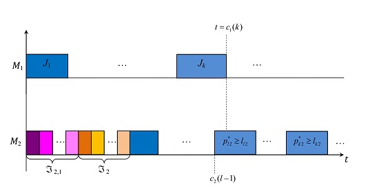
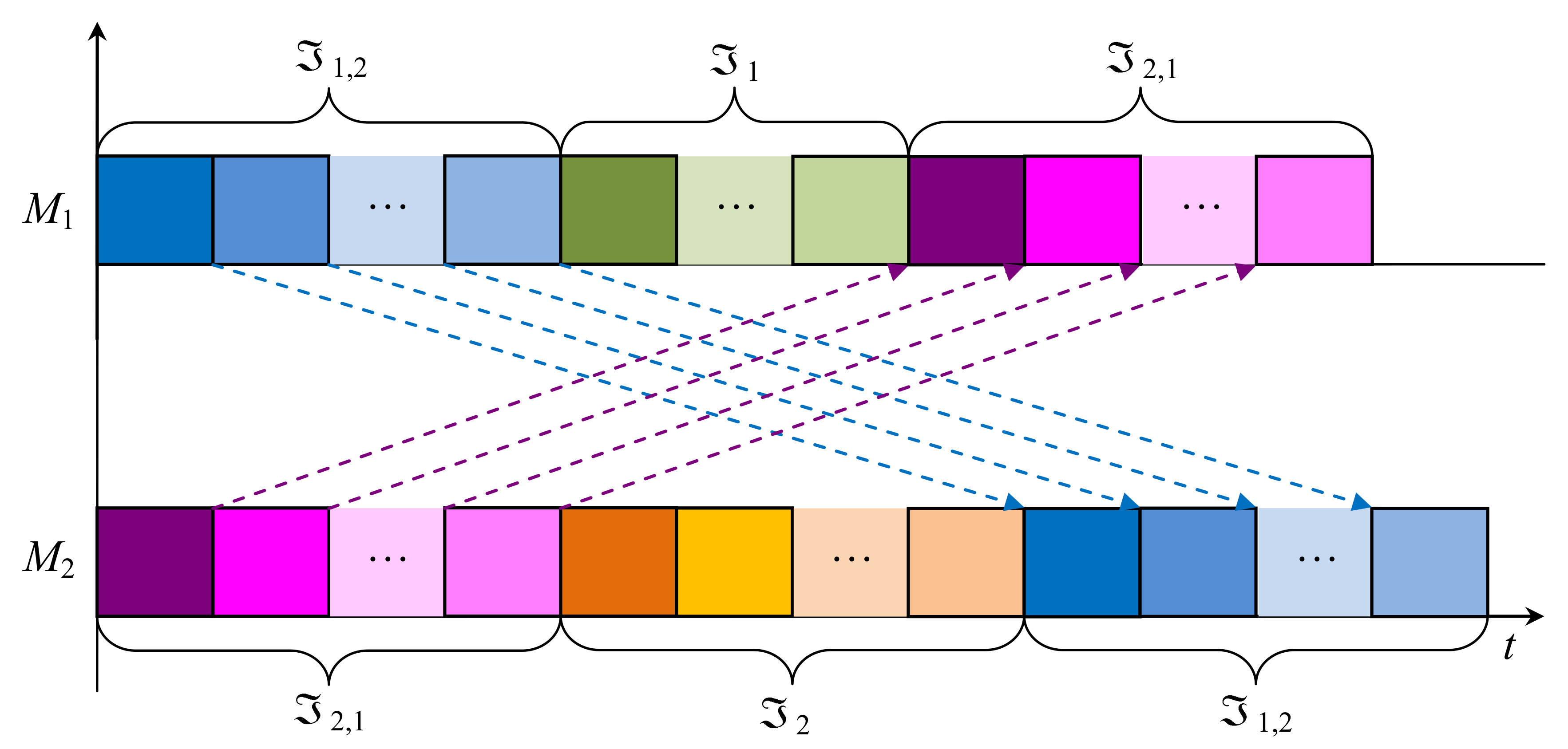
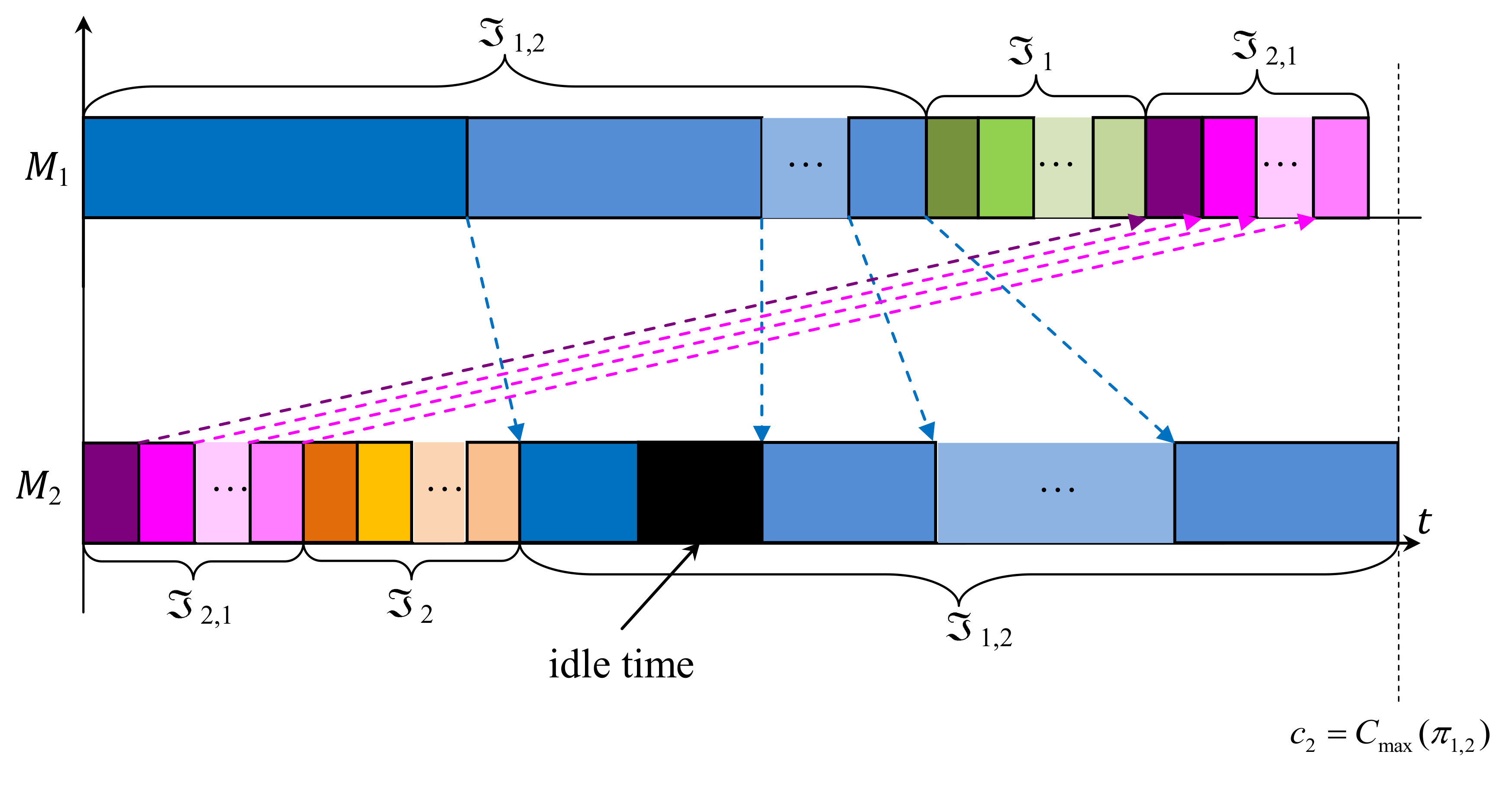
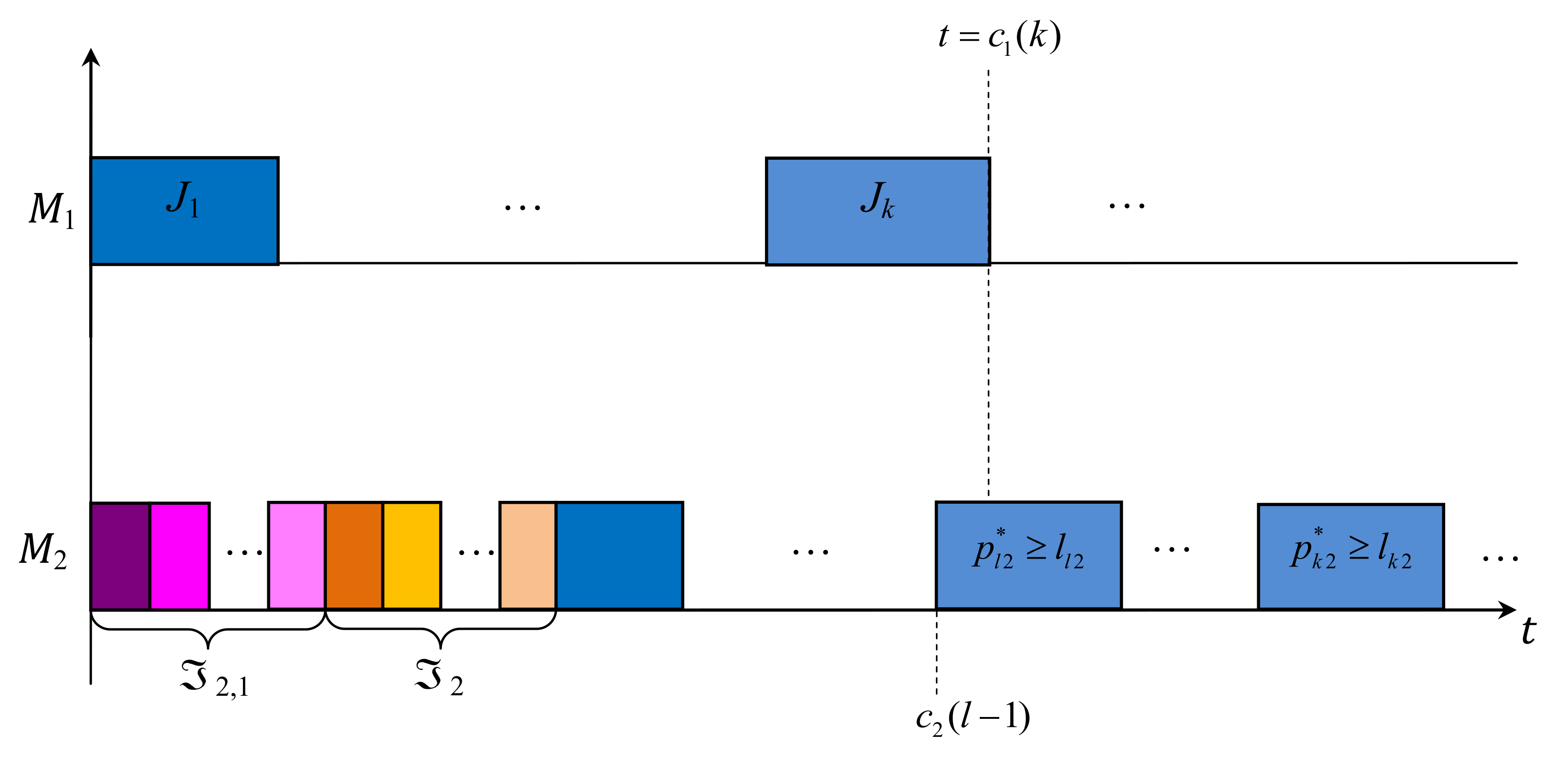
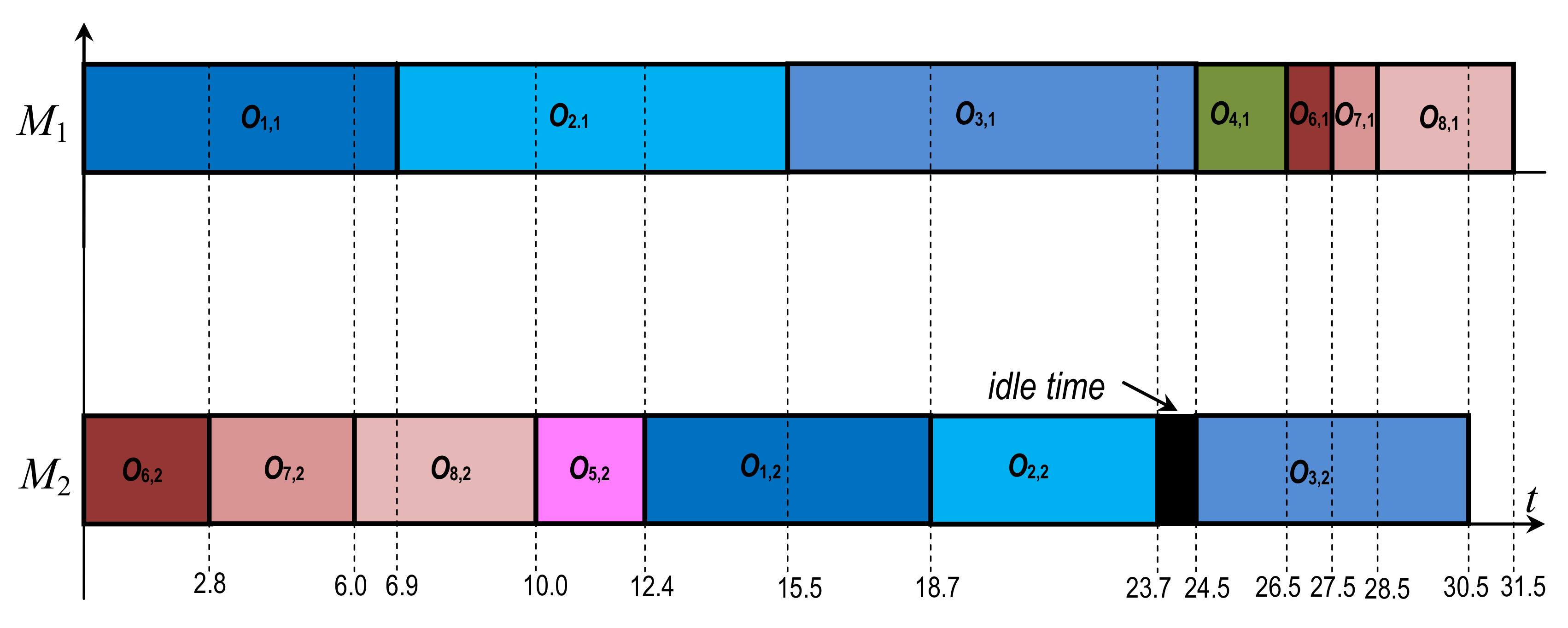
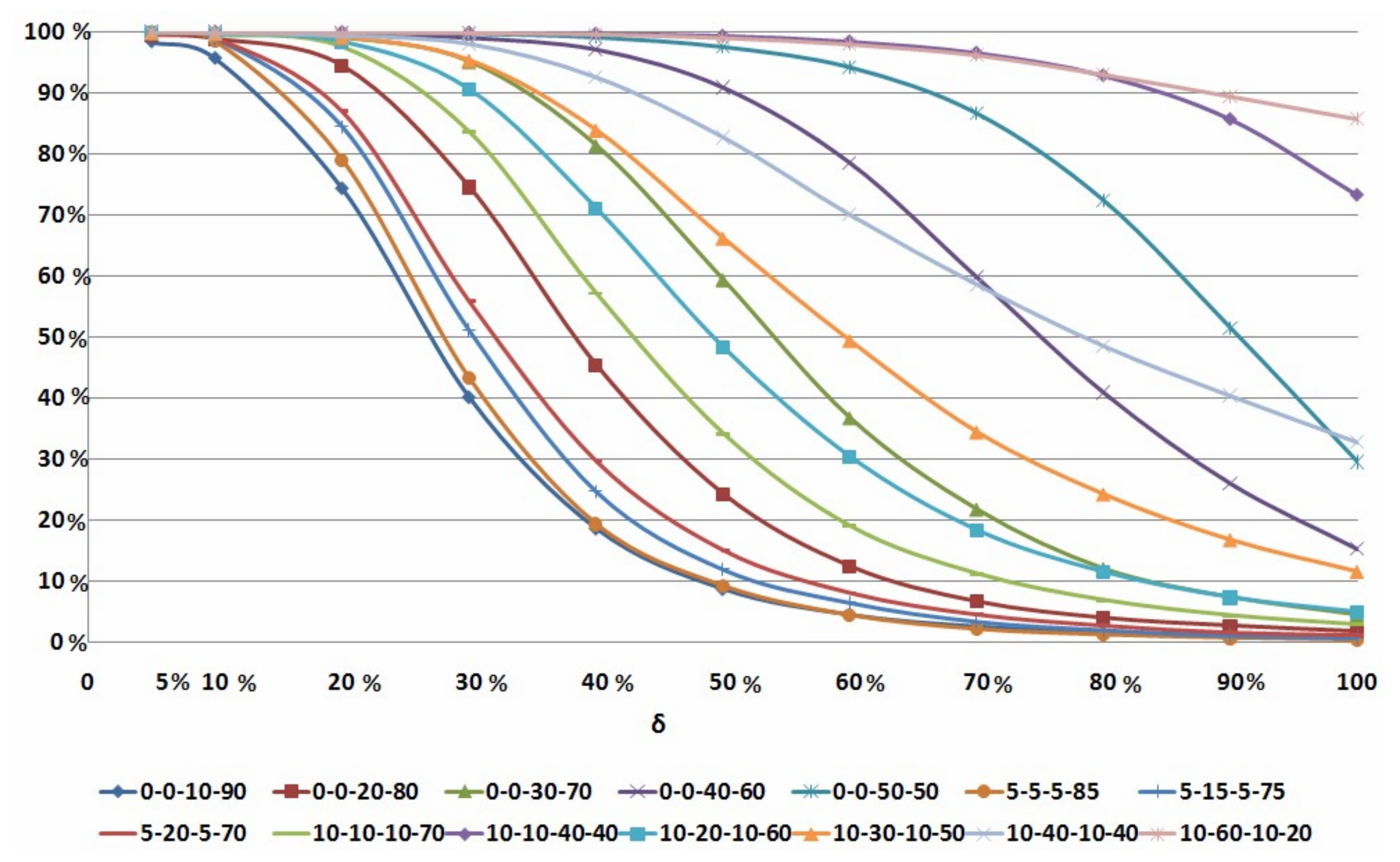
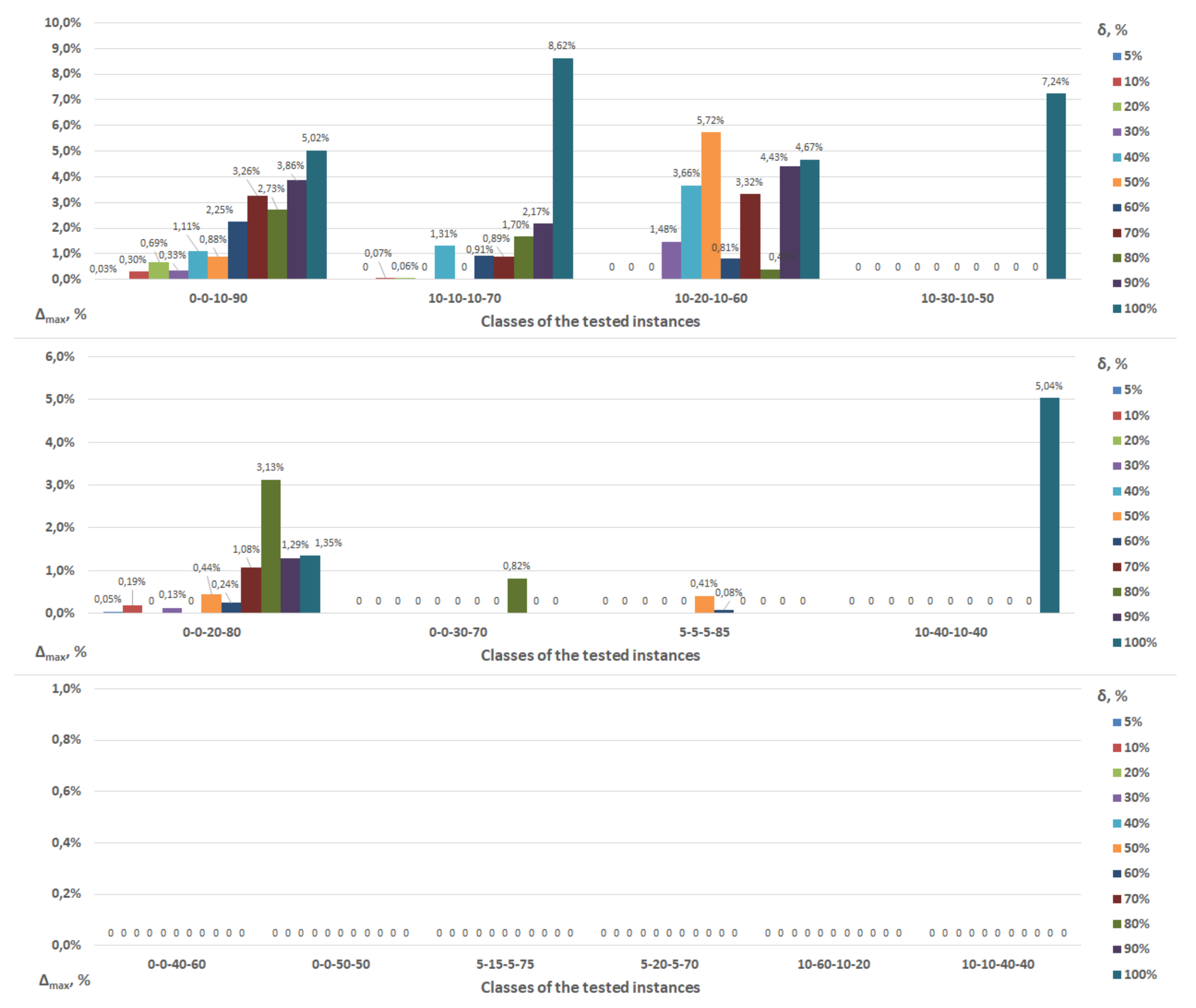
Table A1.
Computational results for the randomly generated instances with the ratio 0%:0%:10%:90% of the numbers of jobs in the subsets , , and of the job set .
Table A1.
Computational results for the randomly generated instances with the ratio 0%:0%:10%:90% of the numbers of jobs in the subsets , , and of the job set .
| Uniform Distributions | Gamma Distributions | ||||||||||||||||||||
|---|---|---|---|---|---|---|---|---|---|---|---|---|---|---|---|---|---|---|---|---|---|
| 10 | 20 | 30 | 40 | 50 | 60 | 70 | 80 | 90 | 100 | 10 | 20 | 30 | 40 | 50 | 60 | 70 | 80 | 90 | 100 | ||
| 5 | Stop1 | 93.9 | 97.3 | 98.4 | 97.6 | 96.6 | 97.6 | 97.9 | 98.3 | 98 | 97.5 | 93.4 | 97 | 97.7 | 97.1 | 98.5 | 98.3 | 97.6 | 98.6 | 98.3 | 98.7 |
| Stop2 | 0.9 | 1 | 0.6 | 1.1 | 1.6 | 1.3 | 1.2 | 1.1 | 0.9 | 1.4 | 0.8 | 0.8 | 0.9 | 1.1 | 0.5 | 0.5 | 1.3 | 0.8 | 0.9 | 0.6 | |
| Stop3 | 5.1 | 1.7 | 1 | 1.3 | 1.8 | 1.1 | 0.9 | 0.6 | 1.1 | 1.1 | 5.3 | 2.2 | 1.4 | 1.8 | 1 | 1.2 | 1.1 | 0.6 | 0.8 | 0.7 | |
| Stop4 | 0.1 | 0 | 0 | 0 | 0 | 0 | 0 | 0 | 0 | 0 | 0.5 | 0 | 0 | 0 | 0 | 0 | 0 | 0 | 0 | 0 | |
| 10 | Stop1 | 85.8 | 91.8 | 91.6 | 93 | 92.2 | 92.2 | 91.9 | 92.6 | 93.6 | 93.8 | 83.1 | 93.5 | 92.8 | 92.7 | 93.1 | 92.3 | 92.4 | 93.3 | 94.2 | 93.6 |
| Stop2 | 2.1 | 2.5 | 4.5 | 3.5 | 4.1 | 4 | 4.2 | 4.6 | 4.2 | 4.2 | 3.2 | 2.8 | 3.1 | 3.5 | 3.6 | 4.3 | 4.2 | 3.4 | 3.5 | 4.1 | |
| Stop3 | 11.7 | 5.7 | 3.9 | 3.5 | 3.7 | 3.8 | 3.9 | 2.8 | 2.2 | 2 | 12.8 | 3.7 | 4.1 | 3.8 | 3.3 | 3.4 | 3.4 | 3.3 | 2.3 | 2.3 | |
| Stop4 | 0.4 | 0 | 0 | 0 | 0 | 0 | 0 | 0 | 0 | 0 | 0.9 | 0 | 0 | 0 | 0 | 0 | 0 | 0 | 0 | 0 | |
| 20 | Stop1 | 70.6 | 73.2 | 73.3 | 71.9 | 69.6 | 63.4 | 63.6 | 57.7 | 56.3 | 53.4 | 70.2 | 73.7 | 74.1 | 71.5 | 67.2 | 64.2 | 63.4 | 61.5 | 56.1 | 57.5 |
| Stop2 | 4.3 | 6.8 | 9.4 | 8.6 | 8.8 | 11.1 | 9.4 | 10.1 | 9.2 | 9.2 | 4.3 | 8.1 | 8.7 | 10 | 10 | 11.3 | 9.1 | 9.1 | 8.9 | 7.5 | |
| Stop3 | 24.2 | 20 | 17.3 | 19.5 | 21.6 | 25.5 | 27 | 32.2 | 34.5 | 37.4 | 24.9 | 18.2 | 17.2 | 18.5 | 22.8 | 24.5 | 27.5 | 29.4 | 35 | 35 | |
| Stop4 | 0.9 | 0 | 0 | 0 | 0 | 0 | 0 | 0 | 0 | 0 | 0.6 | 0 | 0 | 0 | 0 | 0 | 0 | 0 | 0 | 0 | |
| 30 | Stop1 | 53 | 55.1 | 47.5 | 41.1 | 31 | 30.7 | 23.4 | 20.3 | 18.5 | 13.4 | 52 | 52.2 | 44.9 | 34.9 | 33.6 | 26.3 | 27.3 | 18.3 | 18.9 | 14.2 |
| Stop2 | 4.8 | 8.8 | 9.1 | 9.7 | 9.8 | 7 | 6.7 | 5.2 | 4.2 | 4.4 | 6.2 | 8.9 | 10.1 | 10.4 | 11 | 7.9 | 6 | 4.6 | 5.9 | 4.5 | |
| Stop3 | 41.9 | 36.1 | 43.4 | 49.2 | 59.2 | 62.3 | 69.9 | 74.5 | 77.3 | 82.2 | 41 | 38.9 | 45 | 54.7 | 55.4 | 65.8 | 66.7 | 77.1 | 75.2 | 81.3 | |
| Stop4 | 0.3 | 0 | 0 | 0 | 0 | 0 | 0 | 0 | 0 | 0 | 0.8 | 0 | 0 | 0 | 0 | 0 | 0 | 0 | 0 | 0 | |
| 40 | Stop1 | 41.6 | 32.5 | 24.7 | 16.4 | 10.9 | 8.9 | 5.9 | 3.9 | 2.1 | 2.3 | 37.8 | 31.8 | 22.2 | 18.6 | 10.6 | 8.5 | 6.1 | 4.3 | 3 | 1.9 |
| Stop2 | 4.9 | 7.6 | 7.7 | 6.6 | 4.2 | 2.9 | 2 | 1.1 | 0.7 | 0.3 | 5.2 | 8.5 | 9.1 | 4.8 | 2.9 | 3.5 | 2 | 1.6 | 1 | 0.6 | |
| Stop3 | 52.7 | 59.7 | 67.6 | 77 | 84.9 | 88.2 | 92.1 | 95 | 97.2 | 97.4 | 55.3 | 59.7 | 68.7 | 76.6 | 86.5 | 88 | 91.9 | 94.1 | 96 | 97.5 | |
| Stop4 | 0.8 | 0.2 | 0 | 0 | 0 | 0 | 0 | 0 | 0 | 0 | 1.7 | 0 | 0 | 0 | 0 | 0 | 0 | 0 | 0 | 0 | |
| 50 | Stop1 | 29 | 16.1 | 9.3 | 5 | 2.4 | 1.4 | 1.6 | 0.8 | 0.5 | 0 | 26.2 | 19.4 | 10.4 | 5.6 | 3.9 | 1.6 | 0.6 | 0.5 | 0.3 | 0.1 |
| Stop2 | 4.7 | 5.4 | 5 | 2.6 | 1.2 | 0.8 | 0.2 | 0.3 | 0.3 | 0 | 3.7 | 5.6 | 3.8 | 2.2 | 0.7 | 0.7 | 0.7 | 0.1 | 0.2 | 0.1 | |
| Stop3 | 64.9 | 78.5 | 85.7 | 92.4 | 96.4 | 97.8 | 98.2 | 98.9 | 99.2 | 100 | 67.8 | 75 | 85.8 | 92.2 | 95.4 | 97.7 | 98.7 | 99.4 | 99.5 | 99.8 | |
| Stop4 | 1.4 | 0 | 0 | 0 | 0 | 0 | 0 | 0 | 0 | 0 | 2.3 | 0 | 0 | 0 | 0 | 0 | 0 | 0 | 0 | 0 | |
| 60 | Stop1 | 18.1 | 8.4 | 4.6 | 1.4 | 1 | 0.3 | 0.2 | 0.1 | 0 | 0 | 16.6 | 9.6 | 3.6 | 1.4 | 1 | 0.3 | 0 | 0.2 | 0 | 0 |
| Stop2 | 3.8 | 4 | 1.6 | 0.7 | 0.3 | 0.1 | 0 | 0 | 0 | 0 | 3.2 | 3.5 | 2.3 | 0.9 | 0.4 | 0 | 0.3 | 0 | 0.1 | 0 | |
| Stop3 | 76.4 | 87.5 | 93.8 | 97.9 | 98.7 | 99.6 | 99.8 | 99.9 | 100 | 100 | 77.7 | 86.9 | 94.1 | 97.7 | 98.6 | 99.7 | 99.7 | 99.8 | 99.9 | 100 | |
| Stop4 | 1.7 | 0.1 | 0 | 0 | 0 | 0 | 0 | 0 | 0 | 0 | 2.5 | 0 | 0 | 0 | 0 | 0 | 0 | 0 | 0 | 0 | |
| 70 | Stop1 | 12.3 | 5.1 | 1.4 | 0.7 | 0.1 | 0 | 0 | 0 | 0 | 0 | 12.1 | 4.7 | 2.1 | 0.8 | 0.2 | 0 | 0.1 | 0 | 0 | 0 |
| Stop2 | 2.8 | 1.5 | 0.7 | 0.2 | 0.1 | 0 | 0 | 0 | 0 | 0 | 2 | 2.1 | 0.4 | 0.2 | 0 | 0 | 0 | 0 | 0 | 0 | |
| Stop3 | 83.2 | 93.4 | 97.9 | 99.1 | 99.8 | 100 | 100 | 100 | 100 | 100 | 82.8 | 93.2 | 97.5 | 99 | 99.8 | 100 | 99.9 | 100 | 100 | 100 | |
| Stop4 | 1.7 | 0 | 0 | 0 | 0 | 0 | 0 | 0 | 0 | 0 | 3.1 | 0 | 0 | 0 | 0 | 0 | 0 | 0 | 0 | 0 | |
| 80 | Stop1 | 8.9 | 1.9 | 0.4 | 0.3 | 0.2 | 0 | 0 | 0 | 0 | 0 | 10 | 2.3 | 0.6 | 0.2 | 0 | 0 | 0 | 0 | 0 | 0 |
| Stop2 | 1.8 | 0.8 | 0.5 | 0 | 0 | 0 | 0 | 0 | 0 | 0 | 2.2 | 1.1 | 0.2 | 0 | 0 | 0.1 | 0 | 0 | 0 | 0 | |
| Stop3 | 87.1 | 97.1 | 99.1 | 99.7 | 99.8 | 100 | 100 | 100 | 100 | 100 | 84.2 | 96.5 | 99.2 | 99.8 | 100 | 99.9 | 100 | 100 | 100 | 100 | |
| Stop4 | 2.2 | 0.2 | 0 | 0 | 0 | 0 | 0 | 0 | 0 | 0 | 3.6 | 0.1 | 0 | 0 | 0 | 0 | 0 | 0 | 0 | 0 | |
| 90 | Stop1 | 6.9 | 0.8 | 0.2 | 0.1 | 0 | 0 | 0 | 0 | 0 | 0 | 5.7 | 0.9 | 0.3 | 0 | 0 | 0 | 0 | 0 | 0 | 0 |
| Stop2 | 1.2 | 0.7 | 0.1 | 0 | 0 | 0 | 0 | 0 | 0 | 0 | 1.5 | 0.5 | 0 | 0 | 0 | 0 | 0 | 0 | 0 | 0 | |
| Stop3 | 90.1 | 98.4 | 99.7 | 99.9 | 100 | 100 | 100 | 100 | 100 | 100 | 88 | 98.5 | 99.7 | 100 | 100 | 100 | 100 | 100 | 100 | 100 | |
| Stop4 | 1.8 | 0.1 | 0 | 0 | 0 | 0 | 0 | 0 | 0 | 0 | 4.8 | 0.1 | 0 | 0 | 0 | 0 | 0 | 0 | 0 | 0 | |
| 100 | Stop1 | 4.4 | 0.3 | 0.1 | 0.1 | 0 | 0 | 0 | 0 | 0 | 0 | 4.1 | 0.3 | 0 | 0 | 0 | 0 | 0 | 0 | 0 | 0 |
| Stop2 | 1.1 | 0.2 | 0 | 0 | 0 | 0 | 0 | 0 | 0 | 0 | 0.8 | 0 | 0 | 0 | 0 | 0 | 0 | 0 | 0 | 0 | |
| Stop3 | 92.1 | 99.4 | 99.9 | 99.9 | 100 | 100 | 100 | 100 | 100 | 100 | 90.2 | 99.4 | 100 | 100 | 100 | 100 | 100 | 100 | 100 | 100 | |
| Stop4 | 2.4 | 0.1 | 0 | 0 | 0 | 0 | 0 | 0 | 0 | 0 | 4.9 | 0.3 | 0 | 0 | 0 | 0 | 0 | 0 | 0 | 0 | |
Table A2.
Computational results for randomly generated instances with the ratio 0%:0%:20%:80% of the numbers of jobs in the subsets , , and of the job set .
Table A2.
Computational results for randomly generated instances with the ratio 0%:0%:20%:80% of the numbers of jobs in the subsets , , and of the job set .
| Uniform Distributions | Gamma Distributions | ||||||||||||||||||||
|---|---|---|---|---|---|---|---|---|---|---|---|---|---|---|---|---|---|---|---|---|---|
| 10 | 20 | 30 | 40 | 50 | 60 | 70 | 80 | 90 | 100 | 10 | 20 | 30 | 40 | 50 | 60 | 70 | 80 | 90 | 100 | ||
| 5 | Stop1 | 96.7 | 98.9 | 98.6 | 99.5 | 99.7 | 99.7 | 99.9 | 99.9 | 99.9 | 99.9 | 96.7 | 98.9 | 99 | 99.3 | 99.6 | 99.4 | 99.7 | 99.8 | 99.9 | 99.8 |
| Stop2 | 0.8 | 0.3 | 0.7 | 0.1 | 0 | 0.2 | 0.1 | 0.1 | 0.1 | 0.1 | 0.3 | 0.4 | 0.1 | 0.3 | 0.1 | 0.4 | 0.2 | 0.1 | 0.1 | 0.2 | |
| Stop3 | 2.4 | 0.8 | 0.7 | 0.4 | 0.3 | 0.1 | 0 | 0 | 0 | 0 | 3 | 0.7 | 0.9 | 0.4 | 0.3 | 0.2 | 0.1 | 0.1 | 0 | 0 | |
| Stop4 | 0.1 | 0 | 0 | 0 | 0 | 0 | 0 | 0 | 0 | 0 | 0 | 0 | 0 | 0 | 0 | 0 | 0 | 0 | 0 | 0 | |
| 10 | Stop1 | 93.4 | 96.2 | 97.6 | 97.7 | 98 | 98.4 | 98.4 | 98.7 | 98.5 | 99.6 | 93.5 | 96.1 | 97.5 | 97.6 | 97.8 | 98.1 | 98.4 | 98.2 | 99 | 98.7 |
| Stop2 | 1 | 1.4 | 1.4 | 1.4 | 1.4 | 1.3 | 1.1 | 1.2 | 1 | 0.4 | 1 | 1.8 | 1.1 | 1.3 | 1.5 | 1.6 | 1.3 | 1.5 | 0.9 | 1.1 | |
| Stop3 | 5.4 | 2.4 | 1 | 0.9 | 0.6 | 0.3 | 0.5 | 0.1 | 0.5 | 0 | 5.5 | 2.1 | 1.4 | 1.1 | 0.7 | 0.3 | 0.3 | 0.3 | 0.1 | 0.2 | |
| Stop4 | 0.2 | 0 | 0 | 0 | 0 | 0 | 0 | 0 | 0 | 0 | 0 | 0 | 0 | 0 | 0 | 0 | 0 | 0 | 0 | 0 | |
| 20 | Stop1 | 85.4 | 86.9 | 89.5 | 90.2 | 90.8 | 90.5 | 89.1 | 90 | 90.3 | 90.1 | 83.5 | 87.5 | 88.8 | 88.4 | 90.6 | 89.9 | 91 | 89.4 | 90.9 | 90.1 |
| Stop2 | 2.6 | 4.8 | 5.3 | 5 | 5.8 | 5.8 | 5.7 | 5 | 5 | 5.4 | 3.1 | 5.7 | 5.8 | 7.4 | 4.7 | 5.8 | 4.9 | 6.5 | 6.2 | 4 | |
| Stop3 | 12 | 8.3 | 5.2 | 4.8 | 3.4 | 3.7 | 5.2 | 5 | 4.7 | 4.5 | 13.4 | 6.8 | 5.4 | 4.2 | 4.7 | 4.3 | 4.1 | 4.1 | 2.9 | 5.9 | |
| Stop4 | 0 | 0 | 0 | 0 | 0 | 0 | 0 | 0 | 0 | 0 | 0 | 0 | 0 | 0 | 0 | 0 | 0 | 0 | 0 | 0 | |
| 30 | Stop1 | 70.2 | 76.4 | 70.1 | 69.6 | 69.2 | 65.7 | 64.1 | 60.4 | 58 | 56 | 71.6 | 73.3 | 72.9 | 69 | 66 | 63.1 | 60.4 | 62.3 | 62.2 | 58.1 |
| Stop2 | 5.1 | 6.8 | 9.7 | 9.5 | 8.4 | 10.5 | 9.7 | 9.1 | 10.8 | 8.1 | 3.6 | 8.7 | 8.4 | 9.6 | 9.8 | 11.3 | 8.4 | 8.3 | 7.1 | 8.9 | |
| Stop3 | 24.6 | 16.8 | 20.2 | 20.9 | 22.4 | 23.8 | 26.2 | 30.5 | 31.2 | 35.9 | 24.8 | 18 | 18.7 | 21.4 | 24.2 | 25.6 | 31.2 | 29.4 | 30.7 | 33 | |
| Stop4 | 0.1 | 0 | 0 | 0 | 0 | 0 | 0 | 0 | 0 | 0 | 0 | 0 | 0 | 0 | 0 | 0 | 0 | 0 | 0 | 0 | |
| 40 | Stop1 | 56.7 | 55.3 | 48.8 | 41.5 | 39.6 | 31.2 | 31.1 | 26.5 | 23.5 | 21.5 | 55.1 | 53.9 | 46.5 | 41.5 | 37.5 | 31.6 | 33.2 | 27.4 | 26.2 | 21 |
| Stop2 | 5.1 | 8.2 | 10.5 | 10.6 | 9.6 | 8.2 | 7.6 | 6.9 | 7.5 | 5 | 5.6 | 9.2 | 11.5 | 7.7 | 8.9 | 8.7 | 7.3 | 7.2 | 6 | 5.7 | |
| Stop3 | 38.2 | 36.5 | 40.7 | 47.9 | 50.8 | 60.6 | 61.3 | 66.6 | 69 | 73.5 | 39.3 | 36.9 | 42 | 50.8 | 53.6 | 59.7 | 59.5 | 65.4 | 67.8 | 73.3 | |
| Stop4 | 0 | 0 | 0 | 0 | 0 | 0 | 0 | 0 | 0 | 0 | 0 | 0 | 0 | 0 | 0 | 0 | 0 | 0 | 0 | 0 | |
| 50 | Stop1 | 42.6 | 35.2 | 27.2 | 22.9 | 14.3 | 11.4 | 9.9 | 6.9 | 6.6 | 5.9 | 43.9 | 37.3 | 29.2 | 22 | 16.3 | 13.2 | 10.8 | 10.5 | 5.5 | 5.7 |
| Stop2 | 4.4 | 9.5 | 9.8 | 6.5 | 6 | 5.2 | 3.8 | 3.4 | 2.2 | 2.4 | 6 | 10 | 7.3 | 6.9 | 6.5 | 4.8 | 4.7 | 2.8 | 1.9 | 2.5 | |
| Stop3 | 52.8 | 55.3 | 63 | 70.6 | 79.7 | 83.4 | 86.3 | 89.7 | 91.2 | 91.7 | 49.9 | 52.7 | 63.5 | 71.1 | 77.2 | 82 | 84.5 | 86.7 | 92.6 | 91.8 | |
| Stop4 | 0.2 | 0 | 0 | 0 | 0 | 0 | 0 | 0 | 0 | 0 | 0.2 | 0 | 0 | 0 | 0 | 0 | 0 | 0 | 0 | 0 | |
| 60 | Stop1 | 32.9 | 20.7 | 14.4 | 10.7 | 6.3 | 3.3 | 3.3 | 2.2 | 1.4 | 0.8 | 31.7 | 23.1 | 15.7 | 10.4 | 7.2 | 3.9 | 2.9 | 1.4 | 0.9 | 0.6 |
| Stop2 | 5.4 | 5.5 | 4.2 | 2.6 | 2.3 | 1.7 | 0.8 | 0.6 | 0.3 | 0.4 | 5.6 | 6 | 6.4 | 3.6 | 2.4 | 1.5 | 1.5 | 0.8 | 0.3 | 0.7 | |
| Stop3 | 61.7 | 73.8 | 81.4 | 86.7 | 91.4 | 95 | 95.9 | 97.2 | 98.3 | 98.8 | 62.3 | 70.9 | 77.9 | 86 | 90.4 | 94.6 | 95.6 | 97.8 | 98.8 | 98.7 | |
| Stop4 | 0 | 0 | 0 | 0 | 0 | 0 | 0 | 0 | 0 | 0 | 0.4 | 0 | 0 | 0 | 0 | 0 | 0 | 0 | 0 | 0 | |
| 70 | Stop1 | 22.1 | 13.7 | 7.6 | 2.9 | 1.6 | 1.1 | 0.6 | 0.2 | 0.3 | 0.1 | 23.9 | 13.1 | 6.7 | 3.4 | 1.6 | 0.7 | 0.9 | 0.3 | 0.2 | 0.1 |
| Stop2 | 4.9 | 3.7 | 2.9 | 1.7 | 0.9 | 0.6 | 0.4 | 0.1 | 0 | 0.1 | 4.4 | 4.5 | 2 | 1.5 | 1.2 | 0.4 | 0 | 0.4 | 0.1 | 0.1 | |
| Stop3 | 72.8 | 82.6 | 89.5 | 95.4 | 97.5 | 98.3 | 99 | 99.7 | 99.7 | 99.8 | 71.6 | 82.4 | 91.3 | 95.1 | 97.2 | 98.9 | 99.1 | 99.3 | 99.7 | 99.8 | |
| Stop4 | 0.2 | 0 | 0 | 0 | 0 | 0 | 0 | 0 | 0 | 0 | 0.1 | 0 | 0 | 0 | 0 | 0 | 0 | 0 | 0 | 0 | |
| 80 | Stop1 | 17.3 | 8.3 | 3.5 | 1.3 | 0.5 | 0.3 | 0.2 | 0 | 0 | 0 | 16.4 | 7.9 | 3.1 | 1.9 | 0.9 | 0.2 | 0 | 0 | 0 | 0 |
| Stop2 | 2.8 | 1.7 | 1.8 | 0.8 | 0.6 | 0 | 0 | 0 | 0 | 0 | 3.4 | 2.4 | 0.8 | 0.9 | 0.1 | 0.2 | 0.1 | 0 | 0 | 0 | |
| Stop3 | 79.4 | 90 | 94.7 | 97.9 | 98.9 | 99.7 | 99.8 | 100 | 100 | 100 | 79.6 | 89.7 | 96.1 | 97.2 | 99 | 99.6 | 99.9 | 100 | 100 | 100 | |
| Stop4 | 0.5 | 0 | 0 | 0 | 0 | 0 | 0 | 0 | 0 | 0 | 0.6 | 0 | 0 | 0 | 0 | 0 | 0 | 0 | 0 | 0 | |
| 90 | Stop1 | 12.1 | 4.5 | 1.4 | 0.7 | 0 | 0.1 | 0 | 0 | 0 | 0 | 12.6 | 5 | 2.9 | 0.4 | 0.1 | 0.1 | 0 | 0 | 0 | 0 |
| Stop2 | 2.5 | 2.3 | 1.3 | 0.3 | 0 | 0.1 | 0 | 0 | 0 | 0 | 3.2 | 1.8 | 0.2 | 0.2 | 0 | 0 | 0 | 0 | 0 | 0 | |
| Stop3 | 85.2 | 93.2 | 97.3 | 99 | 100 | 99.8 | 100 | 100 | 100 | 100 | 83.7 | 93.2 | 96.9 | 99.4 | 99.9 | 99.9 | 100 | 100 | 100 | 100 | |
| Stop4 | 0.2 | 0 | 0 | 0 | 0 | 0 | 0 | 0 | 0 | 0 | 0.5 | 0 | 0 | 0 | 0 | 0 | 0 | 0 | 0 | 0 | |
| 100 | Stop1 | 10.6 | 2.7 | 0.5 | 0.3 | 0 | 0 | 0 | 0 | 0 | 0 | 9.1 | 2.8 | 0.5 | 0.1 | 0 | 0 | 0 | 0 | 0 | 0 |
| Stop2 | 1.9 | 1.2 | 0.3 | 0 | 0.2 | 0 | 0 | 0 | 0 | 0 | 2 | 0.6 | 0.2 | 0 | 0 | 0 | 0 | 0 | 0 | 0 | |
| Stop3 | 87.4 | 96.1 | 99.2 | 99.7 | 99.8 | 100 | 100 | 100 | 100 | 100 | 88.2 | 96.6 | 99.3 | 99.9 | 100 | 100 | 100 | 100 | 100 | 100 | |
| Stop4 | 0.1 | 0 | 0 | 0 | 0 | 0 | 0 | 0 | 0 | 0 | 0.7 | 0 | 0 | 0 | 0 | 0 | 0 | 0 | 0 | 0 | |
Table A3.
Computational results for randomly generated instances with the ratio 0%:0%:30%:70% of the numbers of jobs in the subsets , , and of the job set .
Table A3.
Computational results for randomly generated instances with the ratio 0%:0%:30%:70% of the numbers of jobs in the subsets , , and of the job set .
| Uniform Distributions | Gamma Distributions | ||||||||||||||||||||
|---|---|---|---|---|---|---|---|---|---|---|---|---|---|---|---|---|---|---|---|---|---|
| 10 | 20 | 30 | 40 | 50 | 60 | 70 | 80 | 90 | 100 | 10 | 20 | 30 | 40 | 50 | 60 | 70 | 80 | 90 | 100 | ||
| 5 | Stop1 | 99.2 | 99.6 | 99.9 | 99.9 | 100 | 100 | 100 | 100 | 100 | 100 | 98.6 | 99.9 | 99.9 | 99.9 | 99.9 | 100 | 100 | 100 | 100 | 100 |
| Stop2 | 0.2 | 0.1 | 0.1 | 0.1 | 0 | 0 | 0 | 0 | 0 | 0 | 0 | 0 | 0 | 0 | 0.1 | 0 | 0 | 0 | 0 | 0 | |
| Stop3 | 0.6 | 0.3 | 0 | 0 | 0 | 0 | 0 | 0 | 0 | 0 | 1.4 | 0.1 | 0.1 | 0.1 | 0 | 0 | 0 | 0 | 0 | 0 | |
| Stop4 | 0 | 0 | 0 | 0 | 0 | 0 | 0 | 0 | 0 | 0 | 0 | 0 | 0 | 0 | 0 | 0 | 0 | 0 | 0 | 0 | |
| 10 | Stop1 | 97.3 | 99 | 99.4 | 99.9 | 99.9 | 100 | 99.9 | 99.9 | 100 | 100 | 97.4 | 98.6 | 99.1 | 99.9 | 99.9 | 100 | 99.9 | 100 | 99.8 | 100 |
| Stop2 | 0.8 | 0.4 | 0.3 | 0.1 | 0.1 | 0 | 0.1 | 0.1 | 0 | 0 | 0.5 | 0.8 | 0.6 | 0.1 | 0.1 | 0 | 0.1 | 0 | 0.2 | 0 | |
| Stop3 | 1.9 | 0.6 | 0.3 | 0 | 0 | 0 | 0 | 0 | 0 | 0 | 2.1 | 0.6 | 0.3 | 0 | 0 | 0 | 0 | 0 | 0 | 0 | |
| Stop4 | 0 | 0 | 0 | 0 | 0 | 0 | 0 | 0 | 0 | 0 | 0 | 0 | 0 | 0 | 0 | 0 | 0 | 0 | 0 | 0 | |
| 20 | Stop1 | 91.7 | 95.7 | 97.1 | 97.5 | 98.2 | 98.6 | 98.7 | 98.7 | 99.7 | 98.9 | 91.5 | 97 | 97.8 | 97.2 | 98.5 | 98.8 | 99.1 | 99.6 | 99.5 | 99.4 |
| Stop2 | 1.9 | 2.6 | 2 | 2.1 | 1.4 | 1.2 | 1.2 | 1.1 | 0.3 | 0.8 | 2.3 | 1.7 | 1.6 | 2.1 | 1.2 | 1 | 0.7 | 0.4 | 0.5 | 0.4 | |
| Stop3 | 6.4 | 1.7 | 0.9 | 0.4 | 0.4 | 0.2 | 0.1 | 0.2 | 0 | 0.3 | 6.2 | 1.3 | 0.6 | 0.7 | 0.3 | 0.2 | 0.2 | 0 | 0 | 0.2 | |
| Stop4 | 0 | 0 | 0 | 0 | 0 | 0 | 0 | 0 | 0 | 0 | 0 | 0 | 0 | 0 | 0 | 0 | 0 | 0 | 0 | 0 | |
| 30 | Stop1 | 81.9 | 87.1 | 89.1 | 91.9 | 91.7 | 92.2 | 92.2 | 93.8 | 93.7 | 93.9 | 83 | 87.2 | 91.7 | 91.7 | 92.4 | 91.6 | 92.2 | 92.8 | 92.9 | 93.4 |
| Stop2 | 4.6 | 6.2 | 5.9 | 4.5 | 5.5 | 4.3 | 4.3 | 3.9 | 2.8 | 2.5 | 3.1 | 5.1 | 4.1 | 4.4 | 3.7 | 4.4 | 4.8 | 4.2 | 3.5 | 3.5 | |
| Stop3 | 13.5 | 6.7 | 5 | 3.6 | 2.8 | 3.5 | 3.5 | 2.3 | 3.5 | 3.6 | 13.9 | 7.7 | 4.2 | 3.9 | 3.9 | 4 | 3 | 3 | 3.6 | 3.1 | |
| Stop4 | 0 | 0 | 0 | 0 | 0 | 0 | 0 | 0 | 0 | 0 | 0 | 0 | 0 | 0 | 0 | 0 | 0 | 0 | 0 | 0 | |
| 40 | Stop1 | 74.1 | 74.7 | 75.9 | 76 | 75.1 | 75.9 | 73.4 | 75.8 | 71.6 | 72.5 | 69.1 | 74.2 | 76.4 | 75.6 | 76.5 | 76.4 | 75 | 74 | 75.3 | 72.7 |
| Stop2 | 4.4 | 7.9 | 7.5 | 8.2 | 6.5 | 6.3 | 6.9 | 5.5 | 6.9 | 7 | 6 | 9.2 | 7.5 | 8 | 7.7 | 6.4 | 6.4 | 7.1 | 4.6 | 6.4 | |
| Stop3 | 21.5 | 17.4 | 16.6 | 15.8 | 18.4 | 17.8 | 19.7 | 18.7 | 21.5 | 20.5 | 24.8 | 16.6 | 16.1 | 16.4 | 15.8 | 17.2 | 18.6 | 18.9 | 20.1 | 20.9 | |
| Stop4 | 0 | 0 | 0 | 0 | 0 | 0 | 0 | 0 | 0 | 0 | 0.1 | 0 | 0 | 0 | 0 | 0 | 0 | 0 | 0 | 0 | |
| 50 | Stop1 | 61.4 | 60.7 | 56.9 | 53.7 | 50.4 | 49.7 | 47.3 | 47.3 | 44.7 | 39.1 | 58.2 | 60.6 | 57.7 | 51.7 | 49.1 | 50.9 | 48.3 | 48.2 | 43.9 | 44.3 |
| Stop2 | 5.3 | 9.2 | 9.7 | 10.4 | 10.2 | 7.7 | 8.4 | 7.1 | 6.7 | 6.3 | 5.8 | 8.7 | 8.5 | 12.4 | 10.2 | 9.1 | 7.8 | 7.1 | 6.6 | 5.3 | |
| Stop3 | 33.3 | 30.1 | 33.4 | 35.9 | 39.4 | 42.6 | 44.3 | 45.6 | 48.6 | 54.6 | 36 | 30.7 | 33.8 | 35.9 | 40.7 | 40 | 43.9 | 44.7 | 49.5 | 50.4 | |
| Stop4 | 0 | 0 | 0 | 0 | 0 | 0 | 0 | 0 | 0 | 0 | 0 | 0 | 0 | 0 | 0 | 0 | 0 | 0 | 0 | 0 | |
| 60 | Stop1 | 46.7 | 46.3 | 39.6 | 32.9 | 30.5 | 29.5 | 23.9 | 22.1 | 18.8 | 17.8 | 50.9 | 42.8 | 41.7 | 35.9 | 30.6 | 28 | 24 | 22.9 | 19 | 13.5 |
| Stop2 | 6.2 | 8.1 | 7.7 | 7.9 | 6.2 | 5.3 | 4.6 | 4.1 | 4.2 | 2.8 | 5 | 9.1 | 7.5 | 7.5 | 7.1 | 5.1 | 5.2 | 4.6 | 3.7 | 3.6 | |
| Stop3 | 47.1 | 45.6 | 52.7 | 59.2 | 63.3 | 65.2 | 71.5 | 73.8 | 77 | 79.4 | 44.1 | 48.1 | 50.8 | 56.6 | 62.3 | 66.9 | 70.8 | 72.5 | 77.3 | 82.9 | |
| Stop4 | 0 | 0 | 0 | 0 | 0 | 0 | 0 | 0 | 0 | 0 | 0 | 0 | 0 | 0 | 0 | 0 | 0 | 0 | 0 | 0 | |
| 70 | Stop1 | 39.9 | 34.5 | 24.5 | 20.2 | 17.6 | 12.2 | 8.7 | 8.6 | 7.6 | 5.5 | 38 | 34.8 | 23.5 | 19.1 | 15.7 | 13.7 | 9.5 | 9 | 6 | 4.7 |
| Stop2 | 5.7 | 7.4 | 6.7 | 5.5 | 4.1 | 2.8 | 2.7 | 1.9 | 1.4 | 0.9 | 6 | 6.8 | 6.3 | 5.6 | 3.9 | 4.8 | 3.4 | 1.4 | 1.4 | 1.3 | |
| Stop3 | 54.4 | 58.1 | 68.8 | 74.3 | 78.3 | 85 | 88.6 | 89.5 | 91 | 93.6 | 55.9 | 58.4 | 70.2 | 75.3 | 80.4 | 81.5 | 87.1 | 89.6 | 92.6 | 94 | |
| Stop4 | 0 | 0 | 0 | 0 | 0 | 0 | 0 | 0 | 0 | 0 | 0.1 | 0 | 0 | 0 | 0 | 0 | 0 | 0 | 0 | 0 | |
| 80 | Stop1 | 27.9 | 21.6 | 14.3 | 8.3 | 7.2 | 4.9 | 4.2 | 2.7 | 0.9 | 0.8 | 28.5 | 21.6 | 14 | 9.5 | 9.3 | 4.2 | 3.9 | 2.2 | 1.2 | 1.5 |
| Stop2 | 4.8 | 5 | 3.6 | 3 | 2.6 | 1.6 | 0.7 | 1 | 0.2 | 0.3 | 5.6 | 5.6 | 5.2 | 3.1 | 1.9 | 2.3 | 1.7 | 0.6 | 0.7 | 0.3 | |
| Stop3 | 67.2 | 73.4 | 82.1 | 88.7 | 90.2 | 93.5 | 95.1 | 96.3 | 98.9 | 98.9 | 65.9 | 72.8 | 80.8 | 87.4 | 88.8 | 93.5 | 94.4 | 97.2 | 98.1 | 98.2 | |
| Stop4 | 0.1 | 0 | 0 | 0 | 0 | 0 | 0 | 0 | 0 | 0 | 0 | 0 | 0 | 0 | 0 | 0 | 0 | 0 | 0 | 0 | |
| 90 | Stop1 | 22.7 | 13.2 | 9.8 | 4.1 | 2.1 | 1.5 | 1.4 | 0.7 | 0.2 | 0 | 23 | 14.4 | 7.4 | 3.6 | 3.4 | 1.9 | 1.2 | 0.7 | 0.3 | 0.9 |
| Stop2 | 3.4 | 4.7 | 3.1 | 1.9 | 1.4 | 0.9 | 0.5 | 0.3 | 0.3 | 0.2 | 3.4 | 5.1 | 2.9 | 2 | 1 | 0.6 | 0.7 | 0.2 | 0.2 | 0.3 | |
| Stop3 | 73.9 | 82.1 | 87.1 | 94 | 96.5 | 97.6 | 98.1 | 99 | 99.5 | 99.8 | 73.4 | 80.5 | 89.7 | 94.4 | 95.6 | 97.5 | 98.1 | 99.1 | 99.5 | 98.8 | |
| Stop4 | 0 | 0 | 0 | 0 | 0 | 0 | 0 | 0 | 0 | 0 | 0.2 | 0 | 0 | 0 | 0 | 0 | 0 | 0 | 0 | 0 | |
| 100 | Stop1 | 17.1 | 8.9 | 3.8 | 2.1 | 1.2 | 0.6 | 0.2 | 0.2 | 0 | 0 | 14.7 | 8 | 4.7 | 2.5 | 1.4 | 0.3 | 0.3 | 0.2 | 0.1 | 0.1 |
| Stop2 | 2.6 | 4.3 | 1.6 | 1.5 | 0.4 | 0.2 | 0.2 | 0 | 0 | 0 | 4.6 | 2.4 | 1.7 | 0.6 | 0.5 | 0.3 | 0.3 | 0.1 | 0.1 | 0 | |
| Stop3 | 80.3 | 86.8 | 94.6 | 96.4 | 98.4 | 99.2 | 99.6 | 99.8 | 100 | 100 | 80.4 | 89.6 | 93.6 | 96.9 | 98.1 | 99.4 | 99.4 | 99.7 | 99.8 | 99.9 | |
| Stop4 | 0 | 0 | 0 | 0 | 0 | 0 | 0 | 0 | 0 | 0 | 0.3 | 0 | 0 | 0 | 0 | 0 | 0 | 0 | 0 | 0 | |
Table A4.
Computational results for randomly generated instances with the ratio 0%:0%:40%:60% of the numbers of jobs in the subsets , , and of the job set .
Table A4.
Computational results for randomly generated instances with the ratio 0%:0%:40%:60% of the numbers of jobs in the subsets , , and of the job set .
| Uniform Distributions | Gamma Distributions | ||||||||||||||||||||
|---|---|---|---|---|---|---|---|---|---|---|---|---|---|---|---|---|---|---|---|---|---|
| 10 | 20 | 30 | 40 | 50 | 60 | 70 | 80 | 90 | 100 | 10 | 20 | 30 | 40 | 50 | 60 | 70 | 80 | 90 | 100 | ||
| 5 | Stop1 | 99.8 | 100 | 100 | 100 | 100 | 100 | 100 | 100 | 100 | 100 | 99.5 | 99.8 | 99.9 | 100 | 99.9 | 100 | 100 | 100 | 100 | 100 |
| Stop2 | 0.1 | 0 | 0 | 0 | 0 | 0 | 0 | 0 | 0 | 0 | 0.1 | 0 | 0.1 | 0 | 0.1 | 0 | 0 | 0 | 0 | 0 | |
| Stop3 | 0.1 | 0 | 0 | 0 | 0 | 0 | 0 | 0 | 0 | 0 | 0.4 | 0.2 | 0 | 0 | 0 | 0 | 0 | 0 | 0 | 0 | |
| Stop4 | 0 | 0 | 0 | 0 | 0 | 0 | 0 | 0 | 0 | 0 | 0 | 0 | 0 | 0 | 0 | 0 | 0 | 0 | 0 | 0 | |
| 10 | Stop1 | 99.2 | 99.7 | 99.9 | 100 | 100 | 100 | 100 | 100 | 100 | 100 | 98.9 | 100 | 99.9 | 100 | 100 | 100 | 100 | 100 | 100 | 100 |
| Stop2 | 0.4 | 0.3 | 0.1 | 0 | 0 | 0 | 0 | 0 | 0 | 0 | 0.2 | 0 | 0.1 | 0 | 0 | 0 | 0 | 0 | 0 | 0 | |
| Stop3 | 0.4 | 0 | 0 | 0 | 0 | 0 | 0 | 0 | 0 | 0 | 0.9 | 0 | 0 | 0 | 0 | 0 | 0 | 0 | 0 | 0 | |
| Stop4 | 0 | 0 | 0 | 0 | 0 | 0 | 0 | 0 | 0 | 0 | 0 | 0 | 0 | 0 | 0 | 0 | 0 | 0 | 0 | 0 | |
| 20 | Stop1 | 96.8 | 98.9 | 99.4 | 99.5 | 99.9 | 99.8 | 100 | 100 | 100 | 99.9 | 96.4 | 98.6 | 99.6 | 99.7 | 99.9 | 100 | 100 | 100 | 100 | 100 |
| Stop2 | 1.1 | 0.6 | 0.4 | 0.5 | 0.1 | 0.2 | 0 | 0 | 0 | 0.1 | 1.6 | 0.8 | 0.4 | 0.3 | 0 | 0 | 0 | 0 | 0 | 0 | |
| Stop3 | 2.1 | 0.5 | 0.2 | 0 | 0 | 0 | 0 | 0 | 0 | 0 | 2 | 0.6 | 0 | 0 | 0.1 | 0 | 0 | 0 | 0 | 0 | |
| Stop4 | 0 | 0 | 0 | 0 | 0 | 0 | 0 | 0 | 0 | 0 | 0 | 0 | 0 | 0 | 0 | 0 | 0 | 0 | 0 | 0 | |
| 30 | Stop1 | 91 | 95.7 | 97.8 | 98.7 | 99.2 | 99.5 | 99.4 | 99.8 | 99.9 | 100 | 91.8 | 94.9 | 97.3 | 98.6 | 99.1 | 99.6 | 99.9 | 99.9 | 99.7 | 100 |
| Stop2 | 3.5 | 1.7 | 1.2 | 0.9 | 0.7 | 0.2 | 0.4 | 0.1 | 0.1 | 0 | 2.3 | 3 | 1.8 | 1.1 | 0.7 | 0.3 | 0.1 | 0.1 | 0.3 | 0 | |
| Stop3 | 5.5 | 2.6 | 1 | 0.4 | 0.1 | 0.3 | 0.2 | 0.1 | 0 | 0 | 5.9 | 2.1 | 0.9 | 0.3 | 0.2 | 0.1 | 0 | 0 | 0 | 0 | |
| Stop4 | 0 | 0 | 0 | 0 | 0 | 0 | 0 | 0 | 0 | 0 | 0 | 0 | 0 | 0 | 0 | 0 | 0 | 0 | 0 | 0 | |
| 40 | Stop1 | 85.8 | 90.4 | 93.7 | 95.1 | 96.4 | 97.6 | 97.2 | 98.2 | 98.3 | 98.5 | 85.4 | 91.2 | 93 | 94.8 | 96.5 | 97.4 | 97.3 | 98 | 98.2 | 98 |
| Stop2 | 2.7 | 4.5 | 3.5 | 1.6 | 1.9 | 1.3 | 2.1 | 0.6 | 1 | 1 | 3.7 | 3.7 | 3.2 | 2.9 | 1.8 | 1.6 | 0.8 | 1.2 | 0.7 | 1.1 | |
| Stop3 | 11.5 | 5.1 | 2.8 | 3.3 | 1.7 | 1.1 | 0.7 | 1.2 | 0.7 | 0.5 | 10.9 | 5.1 | 3.8 | 2.3 | 1.7 | 1 | 1.9 | 0.8 | 1.1 | 0.9 | |
| Stop4 | 0 | 0 | 0 | 0 | 0 | 0 | 0 | 0 | 0 | 0 | 0 | 0 | 0 | 0 | 0 | 0 | 0 | 0 | 0 | 0 | |
| 50 | Stop1 | 75.3 | 82.5 | 84.8 | 87.4 | 87 | 88.2 | 89.7 | 90.7 | 90.5 | 92.3 | 76.3 | 82.5 | 82.4 | 85.4 | 87.5 | 89.7 | 89.6 | 90.4 | 90.7 | 91.3 |
| Stop2 | 5.1 | 5.5 | 6 | 4.4 | 5.1 | 3.8 | 3.7 | 3.3 | 3 | 3 | 4.1 | 5.9 | 6 | 5.9 | 3.9 | 3.5 | 3.3 | 2.4 | 2.7 | 2.4 | |
| Stop3 | 19.6 | 12 | 9.2 | 8.2 | 7.9 | 8 | 6.6 | 6 | 6.5 | 4.7 | 19.6 | 11.6 | 11.6 | 8.7 | 8.6 | 6.8 | 7.1 | 7.2 | 6.6 | 6.3 | |
| Stop4 | 0 | 0 | 0 | 0 | 0 | 0 | 0 | 0 | 0 | 0 | 0 | 0 | 0 | 0 | 0 | 0 | 0 | 0 | 0 | 0 | |
| 60 | Stop1 | 63.4 | 70.1 | 72.3 | 74.7 | 75.8 | 73.9 | 72.5 | 75.4 | 75.4 | 76.6 | 66.3 | 71 | 73.7 | 75.2 | 72.9 | 73.2 | 73.7 | 71.9 | 75.5 | 75.2 |
| Stop2 | 6.6 | 7 | 7.8 | 6.6 | 5.8 | 4.3 | 6.6 | 4.2 | 3.9 | 4.5 | 4.7 | 7.4 | 7 | 5.9 | 5.8 | 5.4 | 4.2 | 5.2 | 5.3 | 3.1 | |
| Stop3 | 30 | 22.9 | 19.9 | 18.7 | 18.4 | 21.8 | 20.9 | 20.4 | 20.7 | 18.9 | 29 | 21.6 | 19.3 | 18.9 | 21.3 | 21.4 | 22.1 | 22.9 | 19.2 | 21.7 | |
| Stop4 | 0 | 0 | 0 | 0 | 0 | 0 | 0 | 0 | 0 | 0 | 0 | 0 | 0 | 0 | 0 | 0 | 0 | 0 | 0 | 0 | |
| 70 | Stop1 | 51.6 | 60 | 57.2 | 55.7 | 56.5 | 52.9 | 50.5 | 50.9 | 50.8 | 50 | 49.5 | 57 | 54.6 | 55.1 | 54.8 | 53.2 | 52.8 | 49.9 | 50 | 51.5 |
| Stop2 | 6.3 | 7.5 | 8.3 | 7.3 | 6.1 | 5.8 | 7.2 | 6.2 | 5.7 | 4.2 | 6.3 | 8.6 | 8 | 7.2 | 6.5 | 5.6 | 7 | 5.9 | 5.2 | 5.7 | |
| Stop3 | 42.1 | 32.5 | 34.5 | 37 | 37.4 | 41.3 | 42.3 | 42.9 | 43.5 | 45.8 | 44.2 | 34.4 | 37.4 | 37.7 | 38.7 | 41.2 | 40.2 | 44.2 | 44.8 | 42.8 | |
| Stop4 | 0 | 0 | 0 | 0 | 0 | 0 | 0 | 0 | 0 | 0 | 0 | 0 | 0 | 0 | 0 | 0 | 0 | 0 | 0 | 0 | |
| 80 | Stop1 | 39.8 | 43.9 | 39.4 | 39 | 37.8 | 34.8 | 31.7 | 31.1 | 30 | 28.1 | 39 | 43.7 | 40.1 | 40.3 | 41.1 | 31.3 | 31.5 | 28.1 | 26 | 28.2 |
| Stop2 | 6.3 | 7.3 | 8.5 | 7.4 | 6.1 | 4.9 | 3.7 | 4.4 | 4.2 | 3.3 | 5.9 | 8.1 | 7.8 | 5.9 | 6.6 | 5.7 | 4.7 | 3.6 | 4.6 | 3 | |
| Stop3 | 53.9 | 48.8 | 52.1 | 53.6 | 56.1 | 60.3 | 64.6 | 64.5 | 65.8 | 68.6 | 55.1 | 48.2 | 52.1 | 53.8 | 52.3 | 63 | 63.8 | 68.3 | 69.4 | 68.8 | |
| Stop4 | 0 | 0 | 0 | 0 | 0 | 0 | 0 | 0 | 0 | 0 | 0 | 0 | 0 | 0 | 0 | 0 | 0 | 0 | 0 | 0 | |
| 90 | Stop1 | 33.7 | 28.9 | 27.6 | 24.1 | 20.7 | 18.2 | 16.8 | 13.5 | 14.1 | 12.4 | 31.7 | 32.1 | 28.8 | 23.8 | 23.8 | 20.1 | 17.1 | 15.9 | 14.2 | 12.3 |
| Stop2 | 6 | 7.7 | 6.9 | 5.3 | 4.5 | 3.3 | 3.6 | 2.8 | 2.6 | 1.7 | 5.7 | 7.1 | 5.9 | 6 | 4.7 | 3.5 | 3.8 | 3 | 3.1 | 1.6 | |
| Stop3 | 60.3 | 63.4 | 65.5 | 70.6 | 74.8 | 78.5 | 79.6 | 83.7 | 83.3 | 85.9 | 62.5 | 60.8 | 65.3 | 70.2 | 71.5 | 76.4 | 79.1 | 81.1 | 82.7 | 86.1 | |
| Stop4 | 0 | 0 | 0 | 0 | 0 | 0 | 0 | 0 | 0 | 0 | 0.1 | 0 | 0 | 0 | 0 | 0 | 0 | 0 | 0 | 0 | |
| 100 | Stop1 | 26.1 | 21.4 | 15.6 | 13.1 | 11.1 | 7.9 | 7.3 | 6 | 4.4 | 4.6 | 24.1 | 21.2 | 16.7 | 16.2 | 11 | 8.2 | 8.3 | 6.7 | 5.7 | 3.8 |
| Stop2 | 3.9 | 6.4 | 5.4 | 4.6 | 3.2 | 2.9 | 1.8 | 1.6 | 0.7 | 1.3 | 5 | 6.2 | 5 | 2.9 | 3.4 | 3.4 | 2.5 | 1.5 | 1.9 | 1 | |
| Stop3 | 70 | 72.2 | 79 | 82.3 | 85.7 | 89.2 | 90.9 | 92.4 | 94.9 | 94.1 | 70.9 | 72.6 | 78.3 | 80.9 | 85.6 | 88.4 | 89.2 | 91.8 | 92.4 | 95.2 | |
| Stop4 | 0 | 0 | 0 | 0 | 0 | 0 | 0 | 0 | 0 | 0 | 0 | 0 | 0 | 0 | 0 | 0 | 0 | 0 | 0 | 0 | |
Table A5.
Computational results for randomly generated instances with the ratio 0%:0%:50%:50% of the numbers of jobs in the subsets , , and of the job set .
Table A5.
Computational results for randomly generated instances with the ratio 0%:0%:50%:50% of the numbers of jobs in the subsets , , and of the job set .
| Uniform Distributions | Gamma Distributions | ||||||||||||||||||||
|---|---|---|---|---|---|---|---|---|---|---|---|---|---|---|---|---|---|---|---|---|---|
| 10 | 20 | 30 | 40 | 50 | 60 | 70 | 80 | 90 | 100 | 10 | 20 | 30 | 40 | 50 | 60 | 70 | 80 | 90 | 100 | ||
| 5 | Stop1 | 100 | 100 | 100 | 100 | 100 | 100 | 100 | 100 | 100 | 100 | 100 | 100 | 100 | 100 | 100 | 100 | 100 | 100 | 100 | 100 |
| Stop2 | 0 | 0 | 0 | 0 | 0 | 0 | 0 | 0 | 0 | 0 | 0 | 0 | 0 | 0 | 0 | 0 | 0 | 0 | 0 | 0 | |
| Stop3 | 0 | 0 | 0 | 0 | 0 | 0 | 0 | 0 | 0 | 0 | 0 | 0 | 0 | 0 | 0 | 0 | 0 | 0 | 0 | 0 | |
| Stop4 | 0 | 0 | 0 | 0 | 0 | 0 | 0 | 0 | 0 | 0 | 0 | 0 | 0 | 0 | 0 | 0 | 0 | 0 | 0 | 0 | |
| 10 | Stop1 | 99.8 | 100 | 100 | 100 | 100 | 100 | 100 | 100 | 100 | 100 | 99.9 | 100 | 100 | 100 | 100 | 100 | 100 | 100 | 100 | 100 |
| Stop2 | 0.1 | 0 | 0 | 0 | 0 | 0 | 0 | 0 | 0 | 0 | 0.1 | 0 | 0 | 0 | 0 | 0 | 0 | 0 | 0 | 0 | |
| Stop3 | 0.1 | 0 | 0 | 0 | 0 | 0 | 0 | 0 | 0 | 0 | 0 | 0 | 0 | 0 | 0 | 0 | 0 | 0 | 0 | 0 | |
| Stop4 | 0 | 0 | 0 | 0 | 0 | 0 | 0 | 0 | 0 | 0 | 0 | 0 | 0 | 0 | 0 | 0 | 0 | 0 | 0 | 0 | |
| 20 | Stop1 | 99.1 | 99.6 | 100 | 100 | 100 | 100 | 100 | 100 | 100 | 100 | 98.9 | 99.9 | 100 | 100 | 100 | 100 | 100 | 100 | 100 | 100 |
| Stop2 | 0.3 | 0.2 | 0 | 0 | 0 | 0 | 0 | 0 | 0 | 0 | 0.5 | 0.1 | 0 | 0 | 0 | 0 | 0 | 0 | 0 | 0 | |
| Stop3 | 0.6 | 0.2 | 0 | 0 | 0 | 0 | 0 | 0 | 0 | 0 | 0.6 | 0 | 0 | 0 | 0 | 0 | 0 | 0 | 0 | 0 | |
| Stop4 | 0 | 0 | 0 | 0 | 0 | 0 | 0 | 0 | 0 | 0 | 0 | 0 | 0 | 0 | 0 | 0 | 0 | 0 | 0 | 0 | |
| 30 | Stop1 | 96.2 | 99.5 | 99.6 | 99.8 | 99.9 | 100 | 100 | 100 | 100 | 100 | 96.1 | 98.7 | 99.8 | 100 | 100 | 100 | 100 | 100 | 100 | 100 |
| Stop2 | 1.5 | 0.5 | 0.4 | 0.2 | 0.1 | 0 | 0 | 0 | 0 | 0 | 1.1 | 1.1 | 0.1 | 0 | 0 | 0 | 0 | 0 | 0 | 0 | |
| Stop3 | 2.3 | 0 | 0 | 0 | 0 | 0 | 0 | 0 | 0 | 0 | 2.8 | 0.2 | 0.1 | 0 | 0 | 0 | 0 | 0 | 0 | 0 | |
| Stop4 | 0 | 0 | 0 | 0 | 0 | 0 | 0 | 0 | 0 | 0 | 0 | 0 | 0 | 0 | 0 | 0 | 0 | 0 | 0 | 0 | |
| 40 | Stop1 | 91.3 | 97.4 | 99.2 | 99.2 | 99.6 | 99.9 | 100 | 100 | 100 | 100 | 91.4 | 96.7 | 98.9 | 99.1 | 99.7 | 99.6 | 99.9 | 100 | 100 | 100 |
| Stop2 | 3 | 1 | 0.2 | 0.5 | 0.1 | 0.1 | 0 | 0 | 0 | 0 | 2.1 | 1.7 | 0.6 | 0.7 | 0.3 | 0.2 | 0.1 | 0 | 0 | 0 | |
| Stop3 | 5.7 | 1.6 | 0.6 | 0.3 | 0.3 | 0 | 0 | 0 | 0 | 0 | 6.5 | 1.6 | 0.5 | 0.2 | 0 | 0.2 | 0 | 0 | 0 | 0 | |
| Stop4 | 0 | 0 | 0 | 0 | 0 | 0 | 0 | 0 | 0 | 0 | 0 | 0 | 0 | 0 | 0 | 0 | 0 | 0 | 0 | 0 | |
| 50 | Stop1 | 83.4 | 92.3 | 95.3 | 97.9 | 98.2 | 98.8 | 99.3 | 99.9 | 99.8 | 100 | 81.7 | 90 | 95.5 | 97.5 | 98.7 | 98.9 | 99.4 | 99.8 | 99.9 | 99.9 |
| Stop2 | 3.5 | 3.3 | 1.9 | 1.1 | 0.9 | 0.6 | 0.1 | 0.1 | 0.1 | 0 | 3.8 | 4.6 | 2.1 | 1.3 | 0.5 | 0.5 | 0.4 | 0 | 0 | 0 | |
| Stop3 | 13.1 | 4.4 | 2.8 | 1 | 0.9 | 0.6 | 0.6 | 0 | 0.1 | 0 | 14.5 | 5.4 | 2.4 | 1.2 | 0.8 | 0.6 | 0.2 | 0.2 | 0.1 | 0.1 | |
| Stop4 | 0 | 0 | 0 | 0 | 0 | 0 | 0 | 0 | 0 | 0 | 0 | 0 | 0 | 0 | 0 | 0 | 0 | 0 | 0 | 0 | |
| 60 | Stop1 | 69.4 | 83.1 | 87.1 | 93.8 | 94.5 | 96.1 | 96.4 | 97.8 | 98.6 | 98.3 | 71.2 | 81.5 | 89.2 | 92.6 | 93.5 | 95.1 | 98 | 98.2 | 98.5 | 98.9 |
| Stop2 | 5.7 | 6.7 | 5 | 2.5 | 2.2 | 1.3 | 0.8 | 0.7 | 0.4 | 0.6 | 6.5 | 6.8 | 3.3 | 3.3 | 2.3 | 2.1 | 0.5 | 0.8 | 0.7 | 0.1 | |
| Stop3 | 24.9 | 10.2 | 7.9 | 3.7 | 3.3 | 2.6 | 2.8 | 1.5 | 1 | 1.1 | 22.3 | 11.7 | 7.5 | 4.1 | 4.2 | 2.8 | 1.5 | 1 | 0.8 | 1 | |
| Stop4 | 0 | 0 | 0 | 0 | 0 | 0 | 0 | 0 | 0 | 0 | 0 | 0 | 0 | 0 | 0 | 0 | 0 | 0 | 0 | 0 | |
| 70 | Stop1 | 59.2 | 70.2 | 75.5 | 81.1 | 81.6 | 88.1 | 87.9 | 92.4 | 92.8 | 93.6 | 58.4 | 72.7 | 74.8 | 81.5 | 85.8 | 87.8 | 88 | 91 | 90.3 | 93.7 |
| Stop2 | 5.8 | 7.4 | 6.6 | 6 | 5.2 | 4.1 | 3.7 | 1.7 | 1.1 | 2.4 | 4.3 | 8.3 | 7.6 | 4.4 | 3.6 | 3.2 | 4.1 | 2.4 | 2.6 | 2 | |
| Stop3 | 35 | 22.4 | 17.9 | 12.9 | 13.2 | 7.8 | 8.4 | 5.9 | 6.1 | 4 | 37.3 | 19 | 17.6 | 14.1 | 10.6 | 9 | 7.9 | 6.6 | 7.1 | 4.3 | |
| Stop4 | 0 | 0 | 0 | 0 | 0 | 0 | 0 | 0 | 0 | 0 | 0 | 0 | 0 | 0 | 0 | 0 | 0 | 0 | 0 | 0 | |
| 80 | Stop1 | 45 | 57.2 | 61.8 | 62.7 | 67.8 | 68.7 | 71 | 74.9 | 75.5 | 77 | 46.8 | 54.8 | 61.1 | 64.1 | 69.4 | 71 | 71.4 | 73.8 | 75.8 | 76 |
| Stop2 | 7 | 8.5 | 7.2 | 7.4 | 7.5 | 6 | 6 | 5.2 | 4.2 | 3.9 | 5.5 | 7.5 | 7 | 7.7 | 6.4 | 5.3 | 6.4 | 4.5 | 4.4 | 3.5 | |
| Stop3 | 48 | 34.3 | 31 | 29.9 | 24.7 | 25.3 | 23 | 19.9 | 20.3 | 19.1 | 47.7 | 37.7 | 31.9 | 28.2 | 24.2 | 23.7 | 22.2 | 21.7 | 19.8 | 20.5 | |
| Stop4 | 0 | 0 | 0 | 0 | 0 | 0 | 0 | 0 | 0 | 0 | 0 | 0 | 0 | 0 | 0 | 0 | 0 | 0 | 0 | 0 | |
| 90 | Stop1 | 35.2 | 41.2 | 38.7 | 44.2 | 42.5 | 45.6 | 46.2 | 45.2 | 50.3 | 50 | 37.2 | 37.3 | 41.3 | 43.8 | 43.3 | 46.5 | 48 | 46.7 | 47.5 | 49.4 |
| Stop2 | 6 | 8.3 | 9.8 | 7.7 | 7.8 | 7.4 | 6.4 | 6.2 | 6.4 | 5.5 | 5.4 | 8.7 | 9.8 | 8.9 | 9.3 | 9.2 | 6.4 | 6.9 | 6.2 | 5.7 | |
| Stop3 | 58.8 | 50.5 | 51.5 | 48.1 | 49.7 | 47 | 47.4 | 48.6 | 43.3 | 44.5 | 57.4 | 54 | 48.9 | 47.3 | 47.4 | 44.3 | 45.6 | 46.4 | 46.3 | 44.9 | |
| Stop4 | 0 | 0 | 0 | 0 | 0 | 0 | 0 | 0 | 0 | 0 | 0 | 0 | 0 | 0 | 0 | 0 | 0 | 0 | 0 | 0 | |
| 100 | Stop1 | 25.7 | 28.8 | 25.2 | 22.6 | 21.4 | 21.4 | 20.2 | 20.5 | 19 | 22.1 | 26.5 | 26 | 25.2 | 25.5 | 25.1 | 22.1 | 22.8 | 19.9 | 23.8 | 20.7 |
| Stop2 | 4.1 | 8.6 | 8.1 | 6.9 | 7.9 | 5.9 | 6.6 | 5.4 | 5.5 | 4.3 | 3.7 | 9.2 | 7.8 | 6 | 7.2 | 7.1 | 5.4 | 5.1 | 4.8 | 4.9 | |
| Stop3 | 70.2 | 62.6 | 66.7 | 70.5 | 70.7 | 72.7 | 73.2 | 74.1 | 75.5 | 73.6 | 69.8 | 64.8 | 67 | 68.5 | 67.7 | 70.8 | 71.8 | 75 | 71.4 | 74.4 | |
| Stop4 | 0 | 0 | 0 | 0 | 0 | 0 | 0 | 0 | 0 | 0 | 0 | 0 | 0 | 0 | 0 | 0 | 0 | 0 | 0 | 0 | |
Table A6.
Computational results for randomly generated instances with the ratio 5%:5%:5%:85% of the numbers of jobs in the subsets , , and of the job set .
Table A6.
Computational results for randomly generated instances with the ratio 5%:5%:5%:85% of the numbers of jobs in the subsets , , and of the job set .
| Uniform Distributions | Gamma Distributions | ||||||||||
|---|---|---|---|---|---|---|---|---|---|---|---|
| 20 | 40 | 60 | 80 | 100 | 20 | 40 | 60 | 80 | 100 | ||
| 5 | Stop1 | 99 | 99.5 | 99.7 | 99.3 | 99.4 | 98.1 | 99.7 | 99.8 | 99.2 | 99.7 |
| Stop2 | 0.3 | 0.3 | 0.2 | 0.4 | 0.6 | 0.4 | 0.2 | 0 | 0.6 | 0.3 | |
| Stop3 | 0.7 | 0.2 | 0.1 | 0.3 | 0 | 1.5 | 0.1 | 0.2 | 0.2 | 0 | |
| Stop4 | 0 | 0 | 0 | 0 | 0 | 0 | 0 | 0 | 0 | 0 | |
| 10 | Stop1 | 96.4 | 97.4 | 98.4 | 97.8 | 97.1 | 95.4 | 97.6 | 97.7 | 98 | 98.6 |
| Stop2 | 0.9 | 1.1 | 0.7 | 1.2 | 0.7 | 1.5 | 1.4 | 1 | 1.3 | 0.3 | |
| Stop3 | 2.7 | 1.5 | 0.9 | 1 | 2.2 | 3.1 | 1 | 1.3 | 0.7 | 1.1 | |
| Stop4 | 0 | 0 | 0 | 0 | 0 | 0 | 0 | 0 | 0 | 0 | |
| 20 | Stop1 | 84.3 | 81.4 | 76.5 | 71.7 | 67.9 | 86.5 | 80.5 | 73.8 | 71 | 66.5 |
| Stop2 | 3.1 | 3.5 | 3.7 | 2.5 | 2.1 | 2.9 | 3.5 | 2.9 | 3.7 | 1.7 | |
| Stop3 | 12.6 | 15.1 | 19.8 | 25.8 | 30 | 10.6 | 16 | 23.3 | 25.3 | 31.8 | |
| Stop4 | 0 | 0 | 0 | 0 | 0 | 0 | 0 | 0 | 0 | 0 | |
| 30 | Stop1 | 61.8 | 52.9 | 38.4 | 27.1 | 20.9 | 65.1 | 53 | 40 | 29.3 | 20.3 |
| Stop2 | 5.7 | 2.9 | 2.1 | 2.1 | 0.3 | 3.4 | 2.6 | 1.4 | 1.4 | 1.2 | |
| Stop3 | 32.5 | 44.2 | 59.5 | 70.8 | 78.8 | 31.4 | 44.4 | 58.6 | 69.3 | 78.5 | |
| Stop4 | 0 | 0 | 0 | 0 | 0 | 0.1 | 0 | 0 | 0 | 0 | |
| 40 | Stop1 | 38.6 | 25.5 | 14.1 | 7.3 | 3.1 | 40 | 24.4 | 13.6 | 6.5 | 3.2 |
| Stop2 | 5.4 | 1.2 | 1.2 | 0.4 | 0.3 | 4.5 | 2.4 | 0.4 | 0.4 | 0.1 | |
| Stop3 | 56 | 73.3 | 84.7 | 92.3 | 96.6 | 55.5 | 73.2 | 86 | 93.1 | 96.7 | |
| Stop4 | 0 | 0 | 0 | 0 | 0 | 0 | 0 | 0 | 0 | 0 | |
| 50 | Stop1 | 27.4 | 8.4 | 3.2 | 1.7 | 0.3 | 25.9 | 10.9 | 3.3 | 0.9 | 0.3 |
| Stop2 | 2.3 | 1.4 | 0.3 | 0 | 0 | 3.7 | 1.1 | 0 | 0 | 0 | |
| Stop3 | 70.2 | 90.2 | 96.5 | 98.3 | 99.7 | 70.4 | 88 | 96.7 | 99.1 | 99.7 | |
| Stop4 | 0.1 | 0 | 0 | 0 | 0 | 0 | 0 | 0 | 0 | 0 | |
| 60 | Stop1 | 14.3 | 3.4 | 0.5 | 0.2 | 0 | 15.7 | 3.2 | 0.6 | 0.3 | 0 |
| Stop2 | 2.3 | 0.4 | 0 | 0 | 0 | 1.8 | 0.1 | 0.3 | 0 | 0 | |
| Stop3 | 83.4 | 96.2 | 99.5 | 99.8 | 100 | 82.4 | 96.7 | 99.1 | 99.7 | 100 | |
| Stop4 | 0 | 0 | 0 | 0 | 0 | 0.1 | 0 | 0 | 0 | 0 | |
| 70 | Stop1 | 8 | 1.1 | 0.3 | 0 | 0 | 6.5 | 1.7 | 0.1 | 0 | 0 |
| Stop2 | 0.9 | 0 | 0 | 0 | 0 | 1.5 | 0 | 0.1 | 0 | 0 | |
| Stop3 | 91.1 | 98.9 | 99.7 | 100 | 100 | 91.8 | 98.3 | 99.8 | 100 | 100 | |
| Stop4 | 0 | 0 | 0 | 0 | 0 | 0.2 | 0 | 0 | 0 | 0 | |
| 80 | Stop1 | 4 | 0.1 | 0 | 0.1 | 0 | 5.1 | 0.2 | 0 | 0 | 0 |
| Stop2 | 0.5 | 0.1 | 0 | 0 | 0 | 0.9 | 0 | 0 | 0 | 0 | |
| Stop3 | 95.5 | 99.8 | 100 | 99.9 | 100 | 93.8 | 99.8 | 100 | 100 | 100 | |
| Stop4 | 0 | 0 | 0 | 0 | 0 | 0.2 | 0 | 0 | 0 | 0 | |
| 90 | Stop1 | 2.6 | 0.3 | 0 | 0 | 0 | 2.2 | 0 | 0 | 0 | 0 |
| Stop2 | 0.3 | 0 | 0 | 0 | 0 | 0.4 | 0 | 0 | 0 | 0 | |
| Stop3 | 97.1 | 99.7 | 100 | 100 | 100 | 97 | 100 | 100 | 100 | 100 | |
| Stop4 | 0 | 0 | 0 | 0 | 0 | 0.4 | 0 | 0 | 0 | 0 | |
| 100 | Stop1 | 0.9 | 0 | 0 | 0 | 0 | 1.5 | 0 | 0 | 0 | 0 |
| Stop2 | 0.3 | 0 | 0 | 0 | 0 | 0 | 0 | 0 | 0 | 0 | |
| Stop3 | 98.8 | 100 | 100 | 100 | 100 | 98.4 | 100 | 100 | 100 | 100 | |
| Stop4 | 0 | 0 | 0 | 0 | 0 | 0.1 | 0 | 0 | 0 | 0 | |
Table A7.
Computational results for randomly generated instances with the ratio 5%:15%:5%:75% of the numbers of jobs in the subsets , , and of the job set .
Table A7.
Computational results for randomly generated instances with the ratio 5%:15%:5%:75% of the numbers of jobs in the subsets , , and of the job set .
| Uniform Distributions | Gamma Distributions | ||||||||||
|---|---|---|---|---|---|---|---|---|---|---|---|
| 20 | 40 | 60 | 80 | 100 | 20 | 40 | 60 | 80 | 100 | ||
| 5 | Stop1 | 98.9 | 99.4 | 99.3 | 99.7 | 99.5 | 98.4 | 99.7 | 99.4 | 99.7 | 99.7 |
| Stop2 | 0.2 | 0.3 | 0.4 | 0.3 | 0.3 | 0.4 | 0.2 | 0.2 | 0.2 | 0.2 | |
| Stop3 | 0.9 | 0.3 | 0.3 | 0 | 0.2 | 1.2 | 0.1 | 0.4 | 0.1 | 0.1 | |
| Stop4 | 0 | 0 | 0 | 0 | 0 | 0 | 0 | 0 | 0 | 0 | |
| 10 | Stop1 | 97 | 98.2 | 97.7 | 98.6 | 99.3 | 95.5 | 98.6 | 98.6 | 98.4 | 98.3 |
| Stop2 | 1 | 0.8 | 1.1 | 0.7 | 0.3 | 1.3 | 0.8 | 0.8 | 0.7 | 0.9 | |
| Stop3 | 2 | 1 | 1.2 | 0.7 | 0.4 | 3.2 | 0.6 | 0.6 | 0.9 | 0.8 | |
| Stop4 | 0 | 0 | 0 | 0 | 0 | 0 | 0 | 0 | 0 | 0 | |
| 20 | Stop1 | 86 | 86.7 | 83.3 | 76.9 | 75.4 | 88.3 | 86.1 | 83.3 | 77.4 | 74.6 |
| Stop2 | 2.6 | 2.8 | 2.5 | 3.1 | 2.5 | 2.5 | 2.3 | 3.1 | 2.7 | 2.3 | |
| Stop3 | 11.4 | 10.5 | 14.2 | 20 | 22.1 | 9.2 | 11.6 | 13.6 | 19.9 | 23.1 | |
| Stop4 | 0 | 0 | 0 | 0 | 0 | 0 | 0 | 0 | 0 | 0 | |
| 30 | Stop1 | 67.1 | 58.1 | 47.1 | 36.1 | 29.3 | 69 | 64.5 | 48.2 | 38.6 | 28.7 |
| Stop2 | 3.1 | 3.2 | 2.8 | 2.6 | 1.5 | 3.2 | 2.1 | 2.2 | 2 | 1.2 | |
| Stop3 | 29.8 | 38.7 | 50.1 | 61.3 | 69.2 | 27.8 | 33.4 | 49.6 | 59.4 | 70.1 | |
| Stop4 | 0 | 0 | 0 | 0 | 0 | 0 | 0 | 0 | 0 | 0 | |
| 40 | Stop1 | 48.2 | 30.1 | 18.9 | 11.1 | 8.3 | 45.6 | 31.8 | 17.6 | 10.5 | 6.6 |
| Stop2 | 2.7 | 3.7 | 1.2 | 0.3 | 0.1 | 4.3 | 2.6 | 1.9 | 0.7 | 0.3 | |
| Stop3 | 49.1 | 66.2 | 79.9 | 88.6 | 91.6 | 50.1 | 65.6 | 80.5 | 88.8 | 93.1 | |
| Stop4 | 0 | 0 | 0 | 0 | 0 | 0 | 0 | 0 | 0 | 0 | |
| 50 | Stop1 | 30.1 | 15.1 | 7.4 | 3 | 1.2 | 29.1 | 13.2 | 6 | 2.7 | 1.7 |
| Stop2 | 2.8 | 1.3 | 0.7 | 0.3 | 0 | 2.6 | 1.1 | 0.3 | 0.2 | 0 | |
| Stop3 | 67.1 | 83.6 | 91.9 | 96.7 | 98.8 | 68.3 | 85.7 | 93.7 | 97.1 | 98.3 | |
| Stop4 | 0 | 0 | 0 | 0 | 0 | 0 | 0 | 0 | 0 | 0 | |
| 60 | Stop1 | 19.2 | 7.6 | 1.9 | 0.5 | 0 | 21.1 | 5.9 | 2.6 | 0.5 | 0.3 |
| Stop2 | 1.5 | 0.4 | 0 | 0 | 0.1 | 2 | 0.5 | 0.2 | 0 | 0 | |
| Stop3 | 79.3 | 92 | 98.1 | 99.5 | 99.9 | 76.9 | 93.6 | 97.2 | 99.5 | 99.7 | |
| Stop4 | 0 | 0 | 0 | 0 | 0 | 0 | 0 | 0 | 0 | 0 | |
| 70 | Stop1 | 11.4 | 2.6 | 0.9 | 0 | 0 | 12 | 3.1 | 0.3 | 0 | 0.1 |
| Stop2 | 1.9 | 0.1 | 0 | 0 | 0 | 0.8 | 0.2 | 0 | 0 | 0 | |
| Stop3 | 86.7 | 97.3 | 99.1 | 100 | 100 | 87.2 | 96.7 | 99.7 | 100 | 99.9 | |
| Stop4 | 0 | 0 | 0 | 0 | 0 | 0 | 0 | 0 | 0 | 0 | |
| 80 | Stop1 | 7.6 | 1.2 | 0.1 | 0 | 0 | 7.9 | 0.6 | 0.2 | 0 | 0 |
| Stop2 | 0.7 | 0.1 | 0 | 0 | 0 | 1 | 0.1 | 0 | 0 | 0 | |
| Stop3 | 91.7 | 98.7 | 99.9 | 100 | 100 | 91.1 | 99.3 | 99.8 | 100 | 100 | |
| Stop4 | 0 | 0 | 0 | 0 | 0 | 0 | 0 | 0 | 0 | 0 | |
| 90 | Stop1 | 3.4 | 0.6 | 0.1 | 0 | 0 | 4.6 | 0.5 | 0.1 | 0 | 0 |
| Stop2 | 0.4 | 0 | 0 | 0 | 0 | 0.5 | 0 | 0 | 0 | 0 | |
| Stop3 | 96.2 | 99.4 | 99.9 | 100 | 100 | 94.9 | 99.5 | 99.9 | 100 | 100 | |
| Stop4 | 0 | 0 | 0 | 0 | 0 | 0 | 0 | 0 | 0 | 0 | |
| 100 | Stop1 | 2.7 | 0.2 | 0 | 0 | 0 | 2.9 | 0.2 | 0 | 0 | 0 |
| Stop2 | 0.5 | 0 | 0 | 0 | 0 | 0.3 | 0 | 0 | 0 | 0 | |
| Stop3 | 96.8 | 99.8 | 100 | 100 | 100 | 96.8 | 99.8 | 100 | 100 | 100 | |
| Stop4 | 0 | 0 | 0 | 0 | 0 | 0 | 0 | 0 | 0 | 0 | |
Table A8.
Computational results for randomly generated instances with the ratio 5%:20%:5%:70% of the numbers of jobs in the subsets , , and of the job set .
Table A8.
Computational results for randomly generated instances with the ratio 5%:20%:5%:70% of the numbers of jobs in the subsets , , and of the job set .
| Uniform Distributions | Gamma Distributions | ||||||||||
|---|---|---|---|---|---|---|---|---|---|---|---|
| 20 | 40 | 60 | 80 | 100 | 20 | 40 | 60 | 80 | 100 | ||
| 5 | Stop1 | 98.6 | 99.2 | 99.6 | 99.4 | 99.5 | 98.3 | 99.2 | 99.7 | 99.8 | 99.6 |
| Stop2 | 0.1 | 0.4 | 0.3 | 0.4 | 0.5 | 0.5 | 0.1 | 0.1 | 0.1 | 0.3 | |
| Stop3 | 1.3 | 0.4 | 0.1 | 0.2 | 0 | 1.2 | 0.7 | 0.2 | 0.1 | 0.1 | |
| Stop4 | 0 | 0 | 0 | 0 | 0 | 0 | 0 | 0 | 0 | 0 | |
| 10 | Stop1 | 96.1 | 98.5 | 99.7 | 99.1 | 99.1 | 96.6 | 98.2 | 98.2 | 98.9 | 98.4 |
| Stop2 | 1.1 | 0.6 | 0.2 | 0.7 | 0.4 | 0.3 | 0.9 | 1.2 | 0.6 | 0.9 | |
| Stop3 | 2.8 | 0.9 | 0.1 | 0.2 | 0.5 | 3.1 | 0.9 | 0.6 | 0.5 | 0.7 | |
| Stop4 | 0 | 0 | 0 | 0 | 0 | 0 | 0 | 0 | 0 | 0 | |
| 20 | Stop1 | 88.8 | 87.6 | 84.6 | 80.1 | 77.6 | 89.5 | 89.8 | 84.6 | 83.5 | 79.3 |
| Stop2 | 1.9 | 2.4 | 2.6 | 2.2 | 2.8 | 3 | 1.9 | 2.7 | 1.9 | 2.4 | |
| Stop3 | 9.3 | 10 | 12.8 | 17.7 | 19.6 | 7.5 | 8.3 | 12.7 | 14.6 | 18.3 | |
| Stop4 | 0 | 0 | 0 | 0 | 0 | 0 | 0 | 0 | 0 | 0 | |
| 30 | Stop1 | 72 | 62.3 | 52.3 | 43.2 | 33.5 | 70.6 | 63.1 | 53 | 42.4 | 36.9 |
| Stop2 | 3.4 | 2.2 | 3.9 | 3 | 1.8 | 3.9 | 3.4 | 3.9 | 2.5 | 0.6 | |
| Stop3 | 24.6 | 35.5 | 43.8 | 53.8 | 64.7 | 25.5 | 33.5 | 43.1 | 55.1 | 62.5 | |
| Stop4 | 0 | 0 | 0 | 0 | 0 | 0 | 0 | 0 | 0 | 0 | |
| 40 | Stop1 | 50.6 | 37.1 | 25.9 | 15 | 9.9 | 50.7 | 36.4 | 25.9 | 16.5 | 10.3 |
| Stop2 | 3.7 | 2.1 | 1.8 | 0.7 | 0.4 | 3.5 | 2.7 | 1.3 | 1 | 0.4 | |
| Stop3 | 45.7 | 60.8 | 72.3 | 84.3 | 89.7 | 45.8 | 60.9 | 72.8 | 82.5 | 89.3 | |
| Stop4 | 0 | 0 | 0 | 0 | 0 | 0 | 0 | 0 | 0 | 0 | |
| 50 | Stop1 | 36.2 | 19.5 | 9.4 | 4.5 | 1.7 | 33.2 | 17.9 | 9.6 | 4.3 | 2.8 |
| Stop2 | 3.1 | 1.6 | 0 | 0.1 | 0.2 | 3.9 | 0.9 | 0.6 | 0.3 | 0 | |
| Stop3 | 60.7 | 78.9 | 90.6 | 95.4 | 98.1 | 62.9 | 81.2 | 89.8 | 95.4 | 97.2 | |
| Stop4 | 0 | 0 | 0 | 0 | 0 | 0 | 0 | 0 | 0 | 0 | |
| 60 | Stop1 | 25.2 | 7.7 | 3.1 | 1.2 | 0.3 | 24 | 7.6 | 3.5 | 0.6 | 0.5 |
| Stop2 | 2 | 0.7 | 0.3 | 0 | 0 | 1.6 | 1.2 | 0.2 | 0 | 0 | |
| Stop3 | 72.8 | 91.6 | 96.6 | 98.8 | 99.7 | 74.4 | 91.2 | 96.3 | 99.4 | 99.5 | |
| Stop4 | 0 | 0 | 0 | 0 | 0 | 0 | 0 | 0 | 0 | 0 | |
| 70 | Stop1 | 12 | 3.3 | 0.8 | 0.2 | 0.4 | 16.6 | 4.1 | 1.6 | 0.5 | 0.1 |
| Stop2 | 2.3 | 0.4 | 0.1 | 0 | 0 | 1.1 | 0.7 | 0 | 0 | 0 | |
| Stop3 | 85.7 | 96.3 | 99.1 | 99.8 | 99.6 | 82.3 | 95.2 | 98.4 | 99.5 | 99.9 | |
| Stop4 | 0 | 0 | 0 | 0 | 0 | 0 | 0 | 0 | 0 | 0 | |
| 80 | Stop1 | 9.4 | 1.8 | 0.3 | 0 | 0 | 9.9 | 1.8 | 0.1 | 0 | 0 |
| Stop2 | 1.4 | 0.1 | 0 | 0 | 0 | 1 | 0.1 | 0 | 0 | 0 | |
| Stop3 | 89.2 | 98.1 | 99.7 | 100 | 100 | 89 | 98.1 | 99.9 | 100 | 100 | |
| Stop4 | 0 | 0 | 0 | 0 | 0 | 0.1 | 0 | 0 | 0 | 0 | |
| 90 | Stop1 | 5.6 | 0.3 | 0.1 | 0.1 | 0 | 6.5 | 0.6 | 0.1 | 0 | 0 |
| Stop2 | 0.7 | 0.1 | 0 | 0 | 0 | 0.3 | 0.1 | 0 | 0 | 0 | |
| Stop3 | 93.7 | 99.6 | 99.9 | 99.9 | 100 | 93.2 | 99.3 | 99.9 | 100 | 100 | |
| Stop4 | 0 | 0 | 0 | 0 | 0 | 0 | 0 | 0 | 0 | 0 | |
| 100 | Stop1 | 4.5 | 0.5 | 0 | 0 | 0 | 4.5 | 0.2 | 0 | 0 | 0 |
| Stop2 | 0.2 | 0 | 0 | 0 | 0 | 0.2 | 0 | 0 | 0 | 0 | |
| Stop3 | 95.3 | 99.5 | 100 | 100 | 100 | 95.3 | 99.8 | 100 | 100 | 100 | |
| Stop4 | 0 | 0 | 0 | 0 | 0 | 0 | 0 | 0 | 0 | 0 | |
Table A9.
Computational results for randomly generated instances with the ratio 10%:10%:10%:70% of the numbers of jobs in the subsets , , and of the job set .
Table A9.
Computational results for randomly generated instances with the ratio 10%:10%:10%:70% of the numbers of jobs in the subsets , , and of the job set .
| Uniform Distributions | Gamma Distributions | ||||||||||||||||||||
|---|---|---|---|---|---|---|---|---|---|---|---|---|---|---|---|---|---|---|---|---|---|
| 10 | 20 | 30 | 40 | 50 | 60 | 70 | 80 | 90 | 100 | 10 | 20 | 30 | 40 | 50 | 60 | 70 | 80 | 90 | 100 | ||
| 5 | Stop1 | 98.9 | 99.5 | 100 | 99.8 | 100 | 99.9 | 100 | 100 | 100 | 99.9 | 98.4 | 99.4 | 99.9 | 100 | 99.9 | 99.9 | 100 | 100 | 100 | 100 |
| Stop2 | 0.4 | 0 | 0 | 0.2 | 0 | 0 | 0 | 0 | 0 | 0.1 | 0 | 0.3 | 0.1 | 0 | 0 | 0.1 | 0 | 0 | 0 | 0 | |
| Stop3 | 0.7 | 0.5 | 0 | 0 | 0 | 0.1 | 0 | 0 | 0 | 0 | 1.6 | 0.3 | 0 | 0 | 0.1 | 0 | 0 | 0 | 0 | 0 | |
| Stop4 | 0 | 0 | 0 | 0 | 0 | 0 | 0 | 0 | 0 | 0 | 0 | 0 | 0 | 0 | 0 | 0 | 0 | 0 | 0 | 0 | |
| 10 | Stop1 | 95.9 | 98.9 | 98.9 | 100 | 99.8 | 100 | 100 | 100 | 99.9 | 99.9 | 96.2 | 98.4 | 99.5 | 99.7 | 99.8 | 99.9 | 99.9 | 99.8 | 99.8 | 99.9 |
| Stop2 | 0.2 | 0.5 | 0.6 | 0 | 0.2 | 0 | 0 | 0 | 0.1 | 0 | 0.3 | 0.3 | 0.2 | 0.1 | 0.1 | 0.1 | 0.1 | 0.2 | 0.2 | 0.1 | |
| Stop3 | 3.8 | 0.6 | 0.5 | 0 | 0 | 0 | 0 | 0 | 0 | 0.1 | 3.4 | 1.3 | 0.3 | 0.2 | 0.1 | 0 | 0 | 0 | 0 | 0 | |
| Stop4 | 0.1 | 0 | 0 | 0 | 0 | 0 | 0 | 0 | 0 | 0 | 0.1 | 0 | 0 | 0 | 0 | 0 | 0 | 0 | 0 | 0 | |
| 20 | Stop1 | 88.8 | 97 | 97.1 | 97.8 | 97.8 | 97.5 | 98.2 | 98.7 | 97.5 | 97.9 | 88.5 | 95.3 | 96.5 | 97.2 | 97.6 | 97.3 | 97.9 | 98.3 | 98.2 | 97.5 |
| Stop2 | 1.6 | 1.2 | 1.1 | 0.5 | 0.6 | 1 | 0.6 | 0.4 | 0.2 | 0.2 | 1.6 | 1.6 | 1 | 1.3 | 0.5 | 0.7 | 0.8 | 0.7 | 0.6 | 0.4 | |
| Stop3 | 9.5 | 1.8 | 1.8 | 1.7 | 1.6 | 1.5 | 1.2 | 0.9 | 2.3 | 1.9 | 9.8 | 3.1 | 2.5 | 1.5 | 1.9 | 2 | 1.3 | 1 | 1.2 | 2.1 | |
| Stop4 | 0.1 | 0 | 0 | 0 | 0 | 0 | 0 | 0 | 0 | 0 | 0.1 | 0 | 0 | 0 | 0 | 0 | 0 | 0 | 0 | 0 | |
| 30 | Stop1 | 79.3 | 85.8 | 86.6 | 85.1 | 81.4 | 83.3 | 82.6 | 79.2 | 77.4 | 75.9 | 80.4 | 86.3 | 86.5 | 85.1 | 81.2 | 81.6 | 80.8 | 80 | 79 | 76.1 |
| Stop2 | 3.7 | 2.2 | 2.5 | 1.7 | 2.9 | 1.8 | 1.5 | 1.2 | 1.5 | 1 | 2.4 | 2.8 | 2.8 | 1.7 | 1.9 | 1.4 | 1.4 | 1.3 | 1 | 0.6 | |
| Stop3 | 17 | 12 | 10.9 | 13.2 | 15.7 | 14.9 | 15.9 | 19.6 | 21.1 | 23.1 | 16.9 | 10.9 | 10.7 | 13.2 | 16.9 | 17 | 17.8 | 18.7 | 20 | 23.3 | |
| Stop4 | 0 | 0 | 0 | 0 | 0 | 0 | 0 | 0 | 0 | 0 | 0.3 | 0 | 0 | 0 | 0 | 0 | 0 | 0 | 0 | 0 | |
| 40 | Stop1 | 66.6 | 71.7 | 65.8 | 62.2 | 58.2 | 53.1 | 48.4 | 44 | 42 | 38.3 | 65.8 | 70.1 | 65.8 | 60.9 | 57.4 | 52.7 | 53.9 | 46.8 | 40.6 | 38.5 |
| Stop2 | 3 | 2.6 | 2.4 | 2.8 | 2.2 | 2.4 | 1.7 | 2 | 1.1 | 0.9 | 2.6 | 2.7 | 2.6 | 1.8 | 1.6 | 1.5 | 2.1 | 1 | 0.9 | 1.1 | |
| Stop3 | 30.2 | 25.7 | 31.8 | 35 | 39.6 | 44.5 | 49.9 | 54 | 56.9 | 60.8 | 31.1 | 27.2 | 31.6 | 37.3 | 41 | 45.8 | 44 | 52.2 | 58.5 | 60.4 | |
| Stop4 | 0.2 | 0 | 0 | 0 | 0 | 0 | 0 | 0 | 0 | 0 | 0.5 | 0 | 0 | 0 | 0 | 0 | 0 | 0 | 0 | 0 | |
| 50 | Stop1 | 55.8 | 55.3 | 46.9 | 38.9 | 30.9 | 25.5 | 22.2 | 19.9 | 15.1 | 13.2 | 56 | 52.9 | 44.3 | 39.4 | 34.1 | 27.4 | 22.6 | 18.2 | 17.5 | 14.9 |
| Stop2 | 2.6 | 2.9 | 2.4 | 2.5 | 1.7 | 1 | 0.8 | 0.3 | 0.7 | 0.6 | 3.3 | 3.5 | 2.4 | 1.4 | 1.7 | 1.1 | 0.7 | 0.5 | 0.4 | 0.7 | |
| Stop3 | 41.6 | 41.8 | 50.7 | 58.6 | 67.4 | 73.5 | 77 | 79.8 | 84.2 | 86.2 | 40.5 | 43.6 | 53.3 | 59.2 | 64.2 | 71.5 | 76.7 | 81.3 | 82.1 | 84.4 | |
| Stop4 | 0 | 0 | 0 | 0 | 0 | 0 | 0 | 0 | 0 | 0 | 0.2 | 0 | 0 | 0 | 0 | 0 | 0 | 0 | 0 | 0 | |
| 60 | Stop1 | 44.4 | 35.9 | 27.8 | 20.1 | 15.6 | 12.7 | 8.6 | 7.1 | 7.8 | 3.3 | 43.6 | 36.5 | 26.2 | 20.7 | 14.6 | 9.9 | 8.8 | 6.4 | 4.2 | 3.2 |
| Stop2 | 3.2 | 2.7 | 1.6 | 0.9 | 0.8 | 0.7 | 0.2 | 0.1 | 0.2 | 0.1 | 3.3 | 2 | 1.4 | 1.8 | 1.7 | 0.2 | 0.2 | 0.3 | 0.1 | 0 | |
| Stop3 | 52.2 | 61.4 | 70.6 | 79 | 83.6 | 86.6 | 91.2 | 92.8 | 92 | 96.6 | 52.5 | 61.5 | 72.4 | 77.5 | 83.7 | 89.9 | 91 | 93.3 | 95.7 | 96.8 | |
| Stop4 | 0.2 | 0 | 0 | 0 | 0 | 0 | 0 | 0 | 0 | 0 | 0.6 | 0 | 0 | 0 | 0 | 0 | 0 | 0 | 0 | 0 | |
| 70 | Stop1 | 33.5 | 25.4 | 17 | 11.2 | 6.6 | 2.8 | 2 | 1.2 | 1.1 | 0.7 | 36.7 | 24 | 17.3 | 11.6 | 5.7 | 5.2 | 3.5 | 1.5 | 0.7 | 1.1 |
| Stop2 | 2.5 | 2 | 1.5 | 0.4 | 0.5 | 0.1 | 0.3 | 0.2 | 0.1 | 0 | 2.4 | 1.9 | 1 | 0.5 | 0.2 | 0.2 | 0 | 0.1 | 0 | 0 | |
| Stop3 | 63.8 | 72.6 | 81.5 | 88.4 | 92.9 | 97.1 | 97.7 | 98.6 | 98.8 | 99.3 | 60.5 | 74.1 | 81.7 | 87.9 | 94.1 | 94.6 | 96.5 | 98.4 | 99.3 | 98.9 | |
| Stop4 | 0.2 | 0 | 0 | 0 | 0 | 0 | 0 | 0 | 0 | 0 | 0.4 | 0 | 0 | 0 | 0 | 0 | 0 | 0 | 0 | 0 | |
| 80 | Stop1 | 29.8 | 13.5 | 10 | 5.1 | 2.9 | 1.2 | 0.3 | 0.4 | 0 | 0.1 | 27.9 | 18.6 | 8.4 | 4 | 2.5 | 1.4 | 0.9 | 0.4 | 0.2 | 0.1 |
| Stop2 | 1.9 | 1.4 | 0.3 | 0.4 | 0.1 | 0 | 0 | 0.1 | 0 | 0 | 2.5 | 0.8 | 0.5 | 0.2 | 0.1 | 0.2 | 0 | 0 | 0 | 0 | |
| Stop3 | 68.1 | 85.1 | 89.7 | 94.5 | 97 | 98.8 | 99.7 | 99.5 | 100 | 99.9 | 68.8 | 80.6 | 91.1 | 95.8 | 97.4 | 98.4 | 99.1 | 99.6 | 99.8 | 99.9 | |
| Stop4 | 0.2 | 0 | 0 | 0 | 0 | 0 | 0 | 0 | 0 | 0 | 0.8 | 0 | 0 | 0 | 0 | 0 | 0 | 0 | 0 | 0 | |
| 90 | Stop1 | 22.4 | 10.5 | 3.9 | 1.7 | 0.7 | 0.1 | 0.3 | 0.2 | 0 | 0 | 20.8 | 10.2 | 4.5 | 3.1 | 0.7 | 0.2 | 0.3 | 0 | 0 | 0 |
| Stop2 | 1.9 | 0.6 | 0.6 | 0.1 | 0 | 0 | 0 | 0 | 0 | 0 | 1.6 | 0.9 | 0.5 | 0 | 0 | 0.1 | 0 | 0 | 0 | 0 | |
| Stop3 | 75.3 | 88.9 | 95.5 | 98.2 | 99.3 | 99.9 | 99.7 | 99.8 | 100 | 100 | 76.8 | 88.9 | 95 | 96.9 | 99.3 | 99.7 | 99.7 | 100 | 100 | 100 | |
| Stop4 | 0.4 | 0 | 0 | 0 | 0 | 0 | 0 | 0 | 0 | 0 | 0.8 | 0 | 0 | 0 | 0 | 0 | 0 | 0 | 0 | 0 | |
| 100 | Stop1 | 15.6 | 5.9 | 1.5 | 0.9 | 0.6 | 0.1 | 0.1 | 0 | 0 | 0 | 15.9 | 6.7 | 2.6 | 0.9 | 0.2 | 0.1 | 0.2 | 0 | 0 | 0 |
| Stop2 | 1.6 | 0.7 | 0.2 | 0 | 0 | 0 | 0 | 0 | 0 | 0 | 1.7 | 0.2 | 0.2 | 0.1 | 0 | 0 | 0 | 0 | 0 | 0 | |
| Stop3 | 82.3 | 93.4 | 98.3 | 99.1 | 99.4 | 99.9 | 99.9 | 100 | 100 | 100 | 81.4 | 93.1 | 97.2 | 99 | 99.8 | 99.9 | 99.8 | 100 | 100 | 100 | |
| Stop4 | 0.5 | 0 | 0 | 0 | 0 | 0 | 0 | 0 | 0 | 0 | 1 | 0 | 0 | 0 | 0 | 0 | 0 | 0 | 0 | 0 | |
Table A10.
Computational results for randomly generated instances with the ratio 10%:10%:40%:40% of the numbers of jobs in the subsets , , and of the job set .
Table A10.
Computational results for randomly generated instances with the ratio 10%:10%:40%:40% of the numbers of jobs in the subsets , , and of the job set .
| Uniform Distributions | Gamma Distributions | ||||||||||||||||||||
|---|---|---|---|---|---|---|---|---|---|---|---|---|---|---|---|---|---|---|---|---|---|
| 10 | 20 | 30 | 40 | 50 | 60 | 70 | 80 | 90 | 100 | 10 | 20 | 30 | 40 | 50 | 60 | 70 | 80 | 90 | 100 | ||
| 5 | Stop1 | 99.9 | 100 | 100 | 100 | 100 | 100 | 100 | 100 | 100 | 100 | 100 | 100 | 100 | 100 | 100 | 100 | 100 | 100 | 100 | 100 |
| Stop2 | 0 | 0 | 0 | 0 | 0 | 0 | 0 | 0 | 0 | 0 | 0 | 0 | 0 | 0 | 0 | 0 | 0 | 0 | 0 | 0 | |
| Stop3 | 0.1 | 0 | 0 | 0 | 0 | 0 | 0 | 0 | 0 | 0 | 0 | 0 | 0 | 0 | 0 | 0 | 0 | 0 | 0 | 0 | |
| Stop4 | 0 | 0 | 0 | 0 | 0 | 0 | 0 | 0 | 0 | 0 | 0 | 0 | 0 | 0 | 0 | 0 | 0 | 0 | 0 | 0 | |
| 10 | Stop1 | 100 | 100 | 100 | 100 | 100 | 100 | 100 | 100 | 100 | 100 | 100 | 100 | 100 | 100 | 100 | 100 | 100 | 100 | 100 | 100 |
| Stop2 | 0 | 0 | 0 | 0 | 0 | 0 | 0 | 0 | 0 | 0 | 0 | 0 | 0 | 0 | 0 | 0 | 0 | 0 | 0 | 0 | |
| Stop3 | 0 | 0 | 0 | 0 | 0 | 0 | 0 | 0 | 0 | 0 | 0 | 0 | 0 | 0 | 0 | 0 | 0 | 0 | 0 | 0 | |
| Stop4 | 0 | 0 | 0 | 0 | 0 | 0 | 0 | 0 | 0 | 0 | 0 | 0 | 0 | 0 | 0 | 0 | 0 | 0 | 0 | 0 | |
| 20 | Stop1 | 99.3 | 100 | 100 | 100 | 100 | 100 | 100 | 100 | 100 | 100 | 99.5 | 100 | 100 | 100 | 100 | 100 | 100 | 100 | 100 | 100 |
| Stop2 | 0.2 | 0 | 0 | 0 | 0 | 0 | 0 | 0 | 0 | 0 | 0.1 | 0 | 0 | 0 | 0 | 0 | 0 | 0 | 0 | 0 | |
| Stop3 | 0.5 | 0 | 0 | 0 | 0 | 0 | 0 | 0 | 0 | 0 | 0.4 | 0 | 0 | 0 | 0 | 0 | 0 | 0 | 0 | 0 | |
| Stop4 | 0 | 0 | 0 | 0 | 0 | 0 | 0 | 0 | 0 | 0 | 0 | 0 | 0 | 0 | 0 | 0 | 0 | 0 | 0 | 0 | |
| 30 | Stop1 | 98.4 | 99.9 | 100 | 100 | 100 | 100 | 100 | 100 | 100 | 100 | 99 | 99.9 | 100 | 100 | 100 | 100 | 100 | 100 | 100 | 100 |
| Stop2 | 0.5 | 0.1 | 0 | 0 | 0 | 0 | 0 | 0 | 0 | 0 | 0.1 | 0 | 0 | 0 | 0 | 0 | 0 | 0 | 0 | 0 | |
| Stop3 | 1.1 | 0 | 0 | 0 | 0 | 0 | 0 | 0 | 0 | 0 | 0.9 | 0.1 | 0 | 0 | 0 | 0 | 0 | 0 | 0 | 0 | |
| Stop4 | 0 | 0 | 0 | 0 | 0 | 0 | 0 | 0 | 0 | 0 | 0 | 0 | 0 | 0 | 0 | 0 | 0 | 0 | 0 | 0 | |
| 40 | Stop1 | 97 | 99.8 | 99.9 | 100 | 100 | 100 | 100 | 100 | 100 | 100 | 96.4 | 99.8 | 100 | 100 | 100 | 100 | 100 | 100 | 100 | 100 |
| Stop2 | 0.1 | 0 | 0.1 | 0 | 0 | 0 | 0 | 0 | 0 | 0 | 0.5 | 0.2 | 0 | 0 | 0 | 0 | 0 | 0 | 0 | 0 | |
| Stop3 | 2.9 | 0.2 | 0 | 0 | 0 | 0 | 0 | 0 | 0 | 0 | 3.1 | 0 | 0 | 0 | 0 | 0 | 0 | 0 | 0 | 0 | |
| Stop4 | 0 | 0 | 0 | 0 | 0 | 0 | 0 | 0 | 0 | 0 | 0 | 0 | 0 | 0 | 0 | 0 | 0 | 0 | 0 | 0 | |
| 50 | Stop1 | 93 | 99 | 99.9 | 99.9 | 100 | 100 | 100 | 100 | 100 | 100 | 92.8 | 99.6 | 99.9 | 100 | 100 | 100 | 100 | 100 | 100 | 100 |
| Stop2 | 1.2 | 0.5 | 0.1 | 0 | 0 | 0 | 0 | 0 | 0 | 0 | 0.9 | 0.1 | 0 | 0 | 0 | 0 | 0 | 0 | 0 | 0 | |
| Stop3 | 5.8 | 0.5 | 0 | 0.1 | 0 | 0 | 0 | 0 | 0 | 0 | 6.3 | 0.3 | 0.1 | 0 | 0 | 0 | 0 | 0 | 0 | 0 | |
| Stop4 | 0 | 0 | 0 | 0 | 0 | 0 | 0 | 0 | 0 | 0 | 0 | 0 | 0 | 0 | 0 | 0 | 0 | 0 | 0 | 0 | |
| 60 | Stop1 | 86.6 | 97.9 | 99.6 | 99.5 | 99.8 | 99.8 | 99.8 | 99.9 | 100 | 100 | 85.8 | 97.1 | 99.3 | 99.6 | 99.8 | 99.7 | 99.9 | 100 | 100 | 100 |
| Stop2 | 1.4 | 0.5 | 0 | 0.2 | 0 | 0.1 | 0 | 0 | 0 | 0 | 1.5 | 0.4 | 0 | 0 | 0 | 0 | 0 | 0 | 0 | 0 | |
| Stop3 | 12 | 1.6 | 0.4 | 0.3 | 0.2 | 0.1 | 0.2 | 0.1 | 0 | 0 | 12.7 | 2.5 | 0.7 | 0.4 | 0.2 | 0.3 | 0.1 | 0 | 0 | 0 | |
| Stop4 | 0 | 0 | 0 | 0 | 0 | 0 | 0 | 0 | 0 | 0 | 0 | 0 | 0 | 0 | 0 | 0 | 0 | 0 | 0 | 0 | |
| 70 | Stop1 | 82.3 | 92.5 | 96.7 | 97.2 | 98.6 | 98.1 | 99 | 99.2 | 99.5 | 99.7 | 80 | 92.7 | 96.5 | 97.5 | 97.9 | 99.2 | 99.5 | 99.5 | 99.8 | 99.5 |
| Stop2 | 1.8 | 1.1 | 0.2 | 0.2 | 0 | 0 | 0.1 | 0 | 0 | 0.1 | 1.7 | 0.5 | 0 | 0.2 | 0.1 | 0 | 0 | 0 | 0 | 0 | |
| Stop3 | 15.9 | 6.4 | 3.1 | 2.6 | 1.4 | 1.9 | 0.9 | 0.8 | 0.5 | 0.2 | 18.3 | 6.8 | 3.5 | 2.3 | 2 | 0.8 | 0.5 | 0.5 | 0.2 | 0.5 | |
| Stop4 | 0 | 0 | 0 | 0 | 0 | 0 | 0 | 0 | 0 | 0 | 0 | 0 | 0 | 0 | 0 | 0 | 0 | 0 | 0 | 0 | |
| 80 | Stop1 | 71.8 | 85.9 | 91.5 | 93.8 | 94.4 | 95.3 | 95.6 | 97.7 | 97.3 | 98.1 | 73.1 | 87.2 | 91 | 93.1 | 95.1 | 95.9 | 96.7 | 97.3 | 98.1 | 98.8 |
| Stop2 | 1.9 | 1.2 | 0.6 | 0.2 | 0.5 | 0 | 0 | 0.1 | 0 | 0.1 | 2 | 0.9 | 0.2 | 0.7 | 0.1 | 0.2 | 0 | 0.3 | 0 | 0 | |
| Stop3 | 26.3 | 12.9 | 7.9 | 6 | 5.1 | 4.7 | 4.4 | 2.2 | 2.7 | 1.8 | 24.9 | 11.9 | 8.8 | 6.2 | 4.8 | 3.9 | 3.3 | 2.4 | 1.9 | 1.2 | |
| Stop4 | 0 | 0 | 0 | 0 | 0 | 0 | 0 | 0 | 0 | 0 | 0 | 0 | 0 | 0 | 0 | 0 | 0 | 0 | 0 | 0 | |
| 90 | Stop1 | 63.2 | 77.8 | 81.6 | 84.2 | 85 | 88.7 | 89.9 | 91.5 | 93.6 | 93.6 | 61.7 | 77.2 | 83.3 | 85 | 86.4 | 88 | 90.4 | 91.4 | 92.7 | 94.4 |
| Stop2 | 2.6 | 1 | 0.8 | 1.1 | 0.2 | 0.2 | 0.6 | 0.2 | 0.1 | 0.2 | 2.6 | 1.9 | 0.9 | 0.2 | 0.5 | 0.2 | 0.1 | 0.1 | 0 | 0.1 | |
| Stop3 | 34.2 | 21.2 | 17.6 | 14.7 | 14.8 | 11.1 | 9.5 | 8.3 | 6.3 | 6.2 | 35.7 | 20.9 | 15.8 | 14.8 | 13.1 | 11.8 | 9.5 | 8.5 | 7.3 | 5.5 | |
| Stop4 | 0 | 0 | 0 | 0 | 0 | 0 | 0 | 0 | 0 | 0 | 0 | 0 | 0 | 0 | 0 | 0 | 0 | 0 | 0 | 0 | |
| 100 | Stop1 | 53.1 | 66.7 | 68.3 | 70.3 | 74.1 | 74.1 | 75.6 | 78.3 | 81 | 84.1 | 51.8 | 67 | 69.8 | 71 | 72.5 | 75.9 | 75.7 | 79.6 | 79.8 | 80.3 |
| Stop2 | 2.1 | 1.7 | 0.6 | 0.8 | 0.3 | 0.7 | 0.3 | 0.2 | 0.1 | 0.3 | 2.4 | 0.9 | 1 | 0.7 | 1.1 | 0.5 | 0.3 | 0.6 | 0.3 | 0.5 | |
| Stop3 | 44.8 | 31.6 | 31.1 | 28.9 | 25.6 | 25.2 | 24.1 | 21.5 | 18.9 | 15.6 | 45.8 | 32.1 | 29.2 | 28.3 | 26.4 | 23.6 | 24 | 19.8 | 19.9 | 19.2 | |
| Stop4 | 0 | 0 | 0 | 0 | 0 | 0 | 0 | 0 | 0 | 0 | 0 | 0 | 0 | 0 | 0 | 0 | 0 | 0 | 0 | 0 | |
Table A11.
Computational results for randomly generated instances with the ratio 10%:20%:10%:60% of the numbers of jobs in the subsets , , and of the job set .
Table A11.
Computational results for randomly generated instances with the ratio 10%:20%:10%:60% of the numbers of jobs in the subsets , , and of the job set .
| Uniform Distributions | Gamma Distributions | ||||||||||||||||||||
|---|---|---|---|---|---|---|---|---|---|---|---|---|---|---|---|---|---|---|---|---|---|
| 10 | 20 | 30 | 40 | 50 | 60 | 70 | 80 | 90 | 100 | 10 | 20 | 30 | 40 | 50 | 60 | 70 | 80 | 90 | 100 | ||
| 5 | Stop1 | 99.2 | 99.6 | 99.8 | 100 | 99.9 | 100 | 100 | 100 | 100 | 100 | 98.5 | 99.8 | 99.9 | 99.9 | 100 | 100 | 100 | 100 | 100 | 100 |
| Stop2 | 0 | 0.1 | 0.2 | 0 | 0.1 | 0 | 0 | 0 | 0 | 0 | 0.2 | 0.1 | 0.1 | 0.1 | 0 | 0 | 0 | 0 | 0 | 0 | |
| Stop3 | 0.8 | 0.3 | 0 | 0 | 0 | 0 | 0 | 0 | 0 | 0 | 1.3 | 0.1 | 0 | 0 | 0 | 0 | 0 | 0 | 0 | 0 | |
| Stop4 | 0 | 0 | 0 | 0 | 0 | 0 | 0 | 0 | 0 | 0 | 0 | 0 | 0 | 0 | 0 | 0 | 0 | 0 | 0 | 0 | |
| 10 | Stop1 | 98.1 | 99.2 | 99.4 | 99.9 | 99.9 | 99.8 | 100 | 100 | 100 | 100 | 96.4 | 99.2 | 99.8 | 99.7 | 99.8 | 99.9 | 99.9 | 100 | 100 | 100 |
| Stop2 | 0.1 | 0.5 | 0.4 | 0.1 | 0.1 | 0 | 0 | 0 | 0 | 0 | 0.6 | 0.3 | 0.2 | 0.1 | 0 | 0.1 | 0.1 | 0 | 0 | 0 | |
| Stop3 | 1.8 | 0.3 | 0.2 | 0 | 0 | 0.2 | 0 | 0 | 0 | 0 | 3 | 0.5 | 0 | 0.2 | 0.2 | 0 | 0 | 0 | 0 | 0 | |
| Stop4 | 0 | 0 | 0 | 0 | 0 | 0 | 0 | 0 | 0 | 0 | 0 | 0 | 0 | 0 | 0 | 0 | 0 | 0 | 0 | 0 | |
| 20 | Stop1 | 91.3 | 97.7 | 97.7 | 97.8 | 99.1 | 98.7 | 98.8 | 98.7 | 99.1 | 99.6 | 90.3 | 96.5 | 97.6 | 98 | 98.4 | 99.1 | 99.4 | 99.4 | 99.2 | 99 |
| Stop2 | 1.4 | 0.8 | 0.8 | 0.7 | 0.4 | 0.7 | 0.4 | 0.4 | 0.1 | 0.1 | 0.3 | 1.3 | 1.4 | 0.9 | 0.7 | 0.6 | 0.1 | 0 | 0.6 | 0.3 | |
| Stop3 | 7.3 | 1.5 | 1.5 | 1.5 | 0.5 | 0.6 | 0.8 | 0.9 | 0.8 | 0.3 | 9.4 | 2.2 | 1 | 1.1 | 0.9 | 0.3 | 0.5 | 0.6 | 0.2 | 0.7 | |
| Stop4 | 0 | 0 | 0 | 0 | 0 | 0 | 0 | 0 | 0 | 0 | 0 | 0 | 0 | 0 | 0 | 0 | 0 | 0 | 0 | 0 | |
| 30 | Stop1 | 83.4 | 90.5 | 92 | 91.4 | 89.7 | 90.8 | 90.4 | 88.7 | 88.8 | 87 | 82.8 | 92.2 | 91.8 | 92.1 | 90.5 | 90.5 | 88.7 | 89.8 | 87.6 | 86.9 |
| Stop2 | 1.7 | 1.7 | 1.7 | 1.1 | 1.2 | 1.6 | 0.6 | 1.4 | 1.1 | 1 | 1.6 | 1.2 | 1.5 | 0.8 | 1.5 | 1.8 | 0.6 | 1.2 | 1.3 | 1.1 | |
| Stop3 | 14.8 | 7.8 | 6.3 | 7.5 | 9.1 | 7.6 | 9 | 9.9 | 10.1 | 12 | 15.6 | 6.6 | 6.7 | 7.1 | 8 | 7.7 | 10.7 | 9 | 11.1 | 12 | |
| Stop4 | 0.1 | 0 | 0 | 0 | 0 | 0 | 0 | 0 | 0 | 0 | 0 | 0 | 0 | 0 | 0 | 0 | 0 | 0 | 0 | 0 | |
| 40 | Stop1 | 75.8 | 78.3 | 76.6 | 74 | 72 | 69.2 | 65.5 | 62.7 | 57.6 | 59.2 | 74.3 | 78.2 | 78.1 | 76.3 | 70.5 | 68.3 | 64 | 65.5 | 61.2 | 58.2 |
| Stop2 | 1.9 | 3 | 3 | 1.9 | 1.6 | 1.4 | 1.8 | 1 | 0.9 | 1.2 | 1.6 | 2.7 | 2.3 | 1.3 | 2.5 | 1.8 | 1.7 | 0.9 | 1.4 | 1.5 | |
| Stop3 | 22 | 18.7 | 20.4 | 24.1 | 26.4 | 29.4 | 32.7 | 36.3 | 41.5 | 39.6 | 24 | 19.1 | 19.6 | 22.4 | 27 | 29.9 | 34.3 | 33.6 | 37.4 | 40.3 | |
| Stop4 | 0.3 | 0 | 0 | 0 | 0 | 0 | 0 | 0 | 0 | 0 | 0.1 | 0 | 0 | 0 | 0 | 0 | 0 | 0 | 0 | 0 | |
| 50 | Stop1 | 64.4 | 65 | 59.6 | 53.1 | 46.9 | 40.6 | 40.1 | 35 | 31.4 | 30.4 | 64.6 | 63.3 | 57.6 | 53.9 | 49.4 | 42.6 | 38.3 | 36.6 | 32.4 | 28 |
| Stop2 | 1.9 | 2.8 | 1.9 | 2.1 | 1.7 | 1.5 | 0.8 | 1.1 | 1.5 | 0.7 | 1.6 | 3.8 | 2.4 | 1.5 | 1.3 | 1.1 | 0.8 | 1.1 | 1.3 | 1.1 | |
| Stop3 | 33.7 | 32.2 | 38.5 | 44.8 | 51.4 | 57.9 | 59.1 | 63.9 | 67.1 | 68.9 | 33.6 | 32.9 | 40 | 44.6 | 49.3 | 56.3 | 60.9 | 62.3 | 66.3 | 70.9 | |
| Stop4 | 0 | 0 | 0 | 0 | 0 | 0 | 0 | 0 | 0 | 0 | 0.2 | 0 | 0 | 0 | 0 | 0 | 0 | 0 | 0 | 0 | |
| 60 | Stop1 | 54.4 | 52.2 | 42.3 | 33 | 28.1 | 21.7 | 19.9 | 15.8 | 13.7 | 11.3 | 54.4 | 49.2 | 43.4 | 33.6 | 26.7 | 22.2 | 20.2 | 14.9 | 13 | 11.1 |
| Stop2 | 1.4 | 2.9 | 1.8 | 1.6 | 1.4 | 0.7 | 0.4 | 0.3 | 0.2 | 0.3 | 2.4 | 2.4 | 2.3 | 2.8 | 0.9 | 0.9 | 0.7 | 0.4 | 0.3 | 0.3 | |
| Stop3 | 44.1 | 44.9 | 55.9 | 65.4 | 70.5 | 77.6 | 79.7 | 83.9 | 86.1 | 88.4 | 43 | 48.4 | 54.3 | 63.6 | 72.4 | 76.9 | 79.1 | 84.7 | 86.7 | 88.6 | |
| Stop4 | 0.1 | 0 | 0 | 0 | 0 | 0 | 0 | 0 | 0 | 0 | 0.2 | 0 | 0 | 0 | 0 | 0 | 0 | 0 | 0 | 0 | |
| 70 | Stop1 | 47 | 37.9 | 25.3 | 21 | 14.1 | 11 | 7.5 | 6 | 4.4 | 3.1 | 44.2 | 34.1 | 28.5 | 19.4 | 14 | 11.3 | 7.5 | 4.4 | 4.1 | 3.1 |
| Stop2 | 1.5 | 1.4 | 1.3 | 1.5 | 0.7 | 0.5 | 0.3 | 0.2 | 0.1 | 0 | 2.1 | 2.9 | 1.4 | 0.7 | 0.9 | 0.4 | 0.1 | 0.2 | 0.1 | 0.1 | |
| Stop3 | 51.5 | 60.7 | 73.4 | 77.5 | 85.2 | 88.5 | 92.2 | 93.8 | 95.5 | 96.9 | 53.4 | 63 | 70.1 | 79.9 | 85.1 | 88.3 | 92.4 | 95.4 | 95.8 | 96.8 | |
| Stop4 | 0 | 0 | 0 | 0 | 0 | 0 | 0 | 0 | 0 | 0 | 0.3 | 0 | 0 | 0 | 0 | 0 | 0 | 0 | 0 | 0 | |
| 80 | Stop1 | 38 | 26.7 | 16 | 10.5 | 6.4 | 4.9 | 2.5 | 1.9 | 0.8 | 0.7 | 35 | 26.1 | 17.6 | 10.4 | 8.1 | 4.2 | 2.2 | 2.1 | 1.3 | 0.5 |
| Stop2 | 1.3 | 1.7 | 1.3 | 1 | 0.9 | 0.1 | 0 | 0.1 | 0 | 0 | 1.6 | 1.3 | 0.7 | 0.7 | 0.3 | 0.4 | 0 | 0 | 0 | 0 | |
| Stop3 | 60.6 | 71.6 | 82.7 | 88.5 | 92.7 | 95 | 97.5 | 98 | 99.2 | 99.3 | 63.1 | 72.6 | 81.7 | 88.9 | 91.6 | 95.4 | 97.8 | 97.9 | 98.7 | 99.5 | |
| Stop4 | 0.1 | 0 | 0 | 0 | 0 | 0 | 0 | 0 | 0 | 0 | 0.3 | 0 | 0 | 0 | 0 | 0 | 0 | 0 | 0 | 0 | |
| 90 | Stop1 | 29 | 15.7 | 9.2 | 4.7 | 3.8 | 1.7 | 1.6 | 0 | 0.2 | 0.3 | 29.5 | 16.7 | 10.2 | 5.9 | 3.2 | 2.1 | 1.1 | 0.7 | 0.3 | 0.2 |
| Stop2 | 1.5 | 1.4 | 0.7 | 0.4 | 0.1 | 0.2 | 0.1 | 0 | 0 | 0.1 | 1.7 | 1.2 | 0.4 | 0.3 | 0 | 0 | 0 | 0 | 0 | 0 | |
| Stop3 | 69.3 | 82.9 | 90.1 | 94.9 | 96.1 | 98.1 | 98.3 | 100 | 99.8 | 99.6 | 68.6 | 82.1 | 89.4 | 93.8 | 96.8 | 97.9 | 98.9 | 99.3 | 99.7 | 99.8 | |
| Stop4 | 0.2 | 0 | 0 | 0 | 0 | 0 | 0 | 0 | 0 | 0 | 0.2 | 0 | 0 | 0 | 0 | 0 | 0 | 0 | 0 | 0 | |
| 100 | Stop1 | 21.6 | 12.2 | 6.7 | 2.4 | 1.6 | 0.6 | 0.2 | 0.1 | 0.1 | 0 | 23 | 11 | 5.8 | 3 | 1.7 | 0.5 | 0.2 | 0.3 | 0 | 0 |
| Stop2 | 1.2 | 0.8 | 0.1 | 0.1 | 0.1 | 0 | 0 | 0 | 0.1 | 0 | 1.1 | 0.6 | 0.5 | 0.2 | 0.1 | 0 | 0 | 0 | 0 | 0 | |
| Stop3 | 77 | 87 | 93.2 | 97.5 | 98.3 | 99.4 | 99.8 | 99.9 | 99.8 | 100 | 75.3 | 88.4 | 93.7 | 96.8 | 98.2 | 99.5 | 99.8 | 99.7 | 100 | 100 | |
| Stop4 | 0.2 | 0 | 0 | 0 | 0 | 0 | 0 | 0 | 0 | 0 | 0.6 | 0 | 0 | 0 | 0 | 0 | 0 | 0 | 0 | 0 | |
Table A12.
Computational results for randomly generated instances with the ratio 10%:30%:10%:50% of the numbers of jobs in the subsets , , and of the job set .
Table A12.
Computational results for randomly generated instances with the ratio 10%:30%:10%:50% of the numbers of jobs in the subsets , , and of the job set .
| Uniform Distributions | Gamma Distributions | ||||||||||||||||||||
|---|---|---|---|---|---|---|---|---|---|---|---|---|---|---|---|---|---|---|---|---|---|
| 10 | 20 | 30 | 40 | 50 | 60 | 70 | 80 | 90 | 100 | 10 | 20 | 30 | 40 | 50 | 60 | 70 | 80 | 90 | 100 | ||
| 5 | Stop1 | 98.6 | 99.9 | 100 | 100 | 100 | 100 | 100 | 100 | 100 | 100 | 99.3 | 100 | 100 | 100 | 100 | 100 | 100 | 100 | 100 | 100 |
| Stop2 | 0.2 | 0 | 0 | 0 | 0 | 0 | 0 | 0 | 0 | 0 | 0 | 0 | 0 | 0 | 0 | 0 | 0 | 0 | 0 | 0 | |
| Stop3 | 1.2 | 0.1 | 0 | 0 | 0 | 0 | 0 | 0 | 0 | 0 | 0.7 | 0 | 0 | 0 | 0 | 0 | 0 | 0 | 0 | 0 | |
| Stop4 | 0 | 0 | 0 | 0 | 0 | 0 | 0 | 0 | 0 | 0 | 0 | 0 | 0 | 0 | 0 | 0 | 0 | 0 | 0 | 0 | |
| 10 | Stop1 | 97.8 | 99.4 | 99.8 | 99.8 | 100 | 99.8 | 100 | 100 | 100 | 100 | 97.3 | 99.7 | 99.7 | 100 | 100 | 99.9 | 100 | 100 | 99.9 | 100 |
| Stop2 | 0.2 | 0.1 | 0.1 | 0.2 | 0 | 0.2 | 0 | 0 | 0 | 0 | 0.2 | 0.1 | 0.1 | 0 | 0 | 0 | 0 | 0 | 0.1 | 0 | |
| Stop3 | 2 | 0.5 | 0.1 | 0 | 0 | 0 | 0 | 0 | 0 | 0 | 2.5 | 0.2 | 0.2 | 0 | 0 | 0.1 | 0 | 0 | 0 | 0 | |
| Stop4 | 0 | 0 | 0 | 0 | 0 | 0 | 0 | 0 | 0 | 0 | 0 | 0 | 0 | 0 | 0 | 0 | 0 | 0 | 0 | 0 | |
| 20 | Stop1 | 93.5 | 98.1 | 98.1 | 99.4 | 99.1 | 99.7 | 99.6 | 99.9 | 99.7 | 99.4 | 95 | 97.5 | 98.8 | 99 | 99.5 | 99.5 | 99.8 | 99.7 | 99.6 | 100 |
| Stop2 | 0.4 | 0.8 | 0.6 | 0.2 | 0.4 | 0.2 | 0.2 | 0.1 | 0.3 | 0.2 | 0.6 | 0.7 | 0.6 | 0.5 | 0.5 | 0.3 | 0.1 | 0.2 | 0.3 | 0 | |
| Stop3 | 6.1 | 1.1 | 1.3 | 0.4 | 0.5 | 0.1 | 0.2 | 0 | 0 | 0.4 | 4.4 | 1.8 | 0.6 | 0.5 | 0 | 0.2 | 0.1 | 0.1 | 0.1 | 0 | |
| Stop4 | 0 | 0 | 0 | 0 | 0 | 0 | 0 | 0 | 0 | 0 | 0 | 0 | 0 | 0 | 0 | 0 | 0 | 0 | 0 | 0 | |
| 30 | Stop1 | 85.9 | 94.2 | 96.1 | 95.2 | 94.3 | 95.3 | 96.1 | 95.8 | 95.8 | 95.2 | 89.9 | 94.2 | 94.2 | 95.3 | 95.4 | 95.9 | 95.2 | 95.2 | 92.8 | 96.3 |
| Stop2 | 0.6 | 1.4 | 1.1 | 1.1 | 1.2 | 0.5 | 0.7 | 1.1 | 0.3 | 0.4 | 0.9 | 0.8 | 1.4 | 1 | 1.5 | 1 | 1.2 | 0.6 | 1.1 | 0.3 | |
| Stop3 | 13.5 | 4.4 | 2.8 | 3.7 | 4.5 | 4.2 | 3.2 | 3.1 | 3.9 | 4.4 | 9.2 | 5 | 4.4 | 3.7 | 3.1 | 3.1 | 3.6 | 4.2 | 6.1 | 3.4 | |
| Stop4 | 0 | 0 | 0 | 0 | 0 | 0 | 0 | 0 | 0 | 0 | 0 | 0 | 0 | 0 | 0 | 0 | 0 | 0 | 0 | 0 | |
| 40 | Stop1 | 80.5 | 85.7 | 85.5 | 83.4 | 85.4 | 81.9 | 82.3 | 77.7 | 77.8 | 77.5 | 81.7 | 85.9 | 88.3 | 85.6 | 82.1 | 84.3 | 81.6 | 79.1 | 80.9 | 80.1 |
| Stop2 | 1.3 | 2.2 | 1.9 | 1.9 | 1.3 | 1.4 | 1.6 | 1.7 | 0.7 | 1.2 | 1.4 | 2.2 | 1.5 | 2.3 | 2 | 1.3 | 0.4 | 1.6 | 1 | 0.9 | |
| Stop3 | 18.2 | 12.1 | 12.6 | 14.7 | 13.3 | 16.7 | 16.1 | 20.6 | 21.5 | 21.3 | 16.9 | 11.9 | 10.2 | 12.1 | 15.9 | 14.4 | 18 | 19.3 | 18.1 | 19 | |
| Stop4 | 0 | 0 | 0 | 0 | 0 | 0 | 0 | 0 | 0 | 0 | 0 | 0 | 0 | 0 | 0 | 0 | 0 | 0 | 0 | 0 | |
| 50 | Stop1 | 74.1 | 74.8 | 72.6 | 70 | 67 | 62 | 59.2 | 58.5 | 54.9 | 52.7 | 73 | 75.9 | 73.6 | 69.7 | 67.6 | 60.9 | 62.6 | 59.1 | 56.6 | 52 |
| Stop2 | 1.2 | 2.6 | 2.5 | 1.8 | 1.3 | 1.5 | 1.5 | 0.9 | 0.9 | 0.6 | 0.9 | 2.1 | 2.1 | 1.3 | 1.2 | 1.1 | 0.8 | 1 | 0.6 | 0.4 | |
| Stop3 | 24.7 | 22.6 | 24.9 | 28.2 | 31.7 | 36.5 | 39.3 | 40.6 | 44.2 | 46.7 | 26.1 | 22 | 24.3 | 29 | 31.2 | 38 | 36.6 | 39.9 | 42.8 | 47.6 | |
| Stop4 | 0 | 0 | 0 | 0 | 0 | 0 | 0 | 0 | 0 | 0 | 0 | 0 | 0 | 0 | 0 | 0 | 0 | 0 | 0 | 0 | |
| 60 | Stop1 | 66.9 | 64.3 | 60.9 | 52.3 | 45 | 46.7 | 40 | 37.4 | 34.6 | 32.2 | 63.8 | 64.2 | 58.4 | 55.9 | 48.2 | 42.8 | 40.1 | 35.9 | 36.3 | 31.2 |
| Stop2 | 1.3 | 3.2 | 1.6 | 2.5 | 1.5 | 0.9 | 1.8 | 0.9 | 0.8 | 0.9 | 0.8 | 2 | 1.9 | 1.6 | 1.8 | 1.4 | 1.2 | 1.3 | 0.9 | 1.3 | |
| Stop3 | 31.8 | 32.5 | 37.5 | 45.2 | 53.5 | 52.4 | 58.2 | 61.7 | 64.6 | 66.9 | 35.4 | 33.8 | 39.7 | 42.5 | 50 | 55.8 | 58.7 | 62.8 | 62.8 | 67.5 | |
| Stop4 | 0 | 0 | 0 | 0 | 0 | 0 | 0 | 0 | 0 | 0 | 0 | 0 | 0 | 0 | 0 | 0 | 0 | 0 | 0 | 0 | |
| 70 | Stop1 | 58.4 | 52.6 | 42.7 | 38.7 | 34.6 | 29.4 | 21.1 | 21.5 | 17.6 | 16.3 | 57.7 | 50.8 | 45 | 37.9 | 31 | 27.6 | 26.2 | 21.6 | 20.5 | 15.1 |
| Stop2 | 1.4 | 2.2 | 1 | 2.3 | 0.8 | 0.7 | 0.5 | 0.3 | 0.2 | 0.1 | 0.9 | 3.5 | 2.4 | 1.1 | 1.3 | 0.6 | 0.6 | 0.4 | 0.3 | 0 | |
| Stop3 | 40.2 | 45.2 | 56.3 | 59 | 64.6 | 69.9 | 78.4 | 78.2 | 82.2 | 83.6 | 41.3 | 45.7 | 52.6 | 61 | 67.7 | 71.8 | 73.2 | 78 | 79.2 | 84.9 | |
| Stop4 | 0 | 0 | 0 | 0 | 0 | 0 | 0 | 0 | 0 | 0 | 0.1 | 0 | 0 | 0 | 0 | 0 | 0 | 0 | 0 | 0 | |
| 80 | Stop1 | 51.9 | 40.7 | 34.1 | 28.3 | 21.4 | 14.2 | 13.9 | 9.9 | 9.8 | 8 | 49.7 | 41.7 | 33.3 | 27.1 | 24.1 | 17.4 | 14.1 | 12.6 | 8.8 | 7.5 |
| Stop2 | 0.9 | 1.7 | 1.4 | 1.4 | 0.2 | 0.1 | 0.2 | 0.3 | 0.1 | 0 | 0.8 | 2.5 | 1.6 | 0.9 | 0.5 | 0.3 | 0.6 | 0.5 | 0 | 0 | |
| Stop3 | 47.2 | 57.6 | 64.5 | 70.3 | 78.4 | 85.7 | 85.9 | 89.8 | 90.1 | 92 | 49.4 | 55.8 | 65.1 | 72 | 75.4 | 82.3 | 85.3 | 86.9 | 91.2 | 92.5 | |
| Stop4 | 0 | 0 | 0 | 0 | 0 | 0 | 0 | 0 | 0 | 0 | 0.1 | 0 | 0 | 0 | 0 | 0 | 0 | 0 | 0 | 0 | |
| 90 | Stop1 | 44.2 | 31.3 | 24.6 | 17.3 | 12.3 | 11 | 7.1 | 4.7 | 3.6 | 4.2 | 44 | 32.7 | 24.8 | 16.3 | 12.7 | 10 | 7.9 | 6.5 | 4.2 | 3.8 |
| Stop2 | 1.3 | 1.3 | 0.4 | 0.8 | 0.2 | 0.1 | 0.1 | 0.1 | 0.1 | 0 | 1 | 1.4 | 1.2 | 1 | 0.3 | 0 | 0.1 | 0 | 0.1 | 0.1 | |
| Stop3 | 54.5 | 67.4 | 75 | 81.9 | 87.5 | 88.9 | 92.8 | 95.2 | 96.3 | 95.8 | 54.6 | 65.9 | 74 | 82.7 | 87 | 90 | 92 | 93.5 | 95.7 | 96.1 | |
| Stop4 | 0 | 0 | 0 | 0 | 0 | 0 | 0 | 0 | 0 | 0 | 0.4 | 0 | 0 | 0 | 0 | 0 | 0 | 0 | 0 | 0 | |
| 100 | Stop1 | 36.1 | 24.3 | 17.8 | 12.4 | 7.5 | 6.2 | 3 | 2.9 | 2.3 | 1.1 | 35.5 | 25.9 | 15.3 | 10.6 | 6.9 | 5.1 | 3.1 | 2 | 1.8 | 1.7 |
| Stop2 | 0.8 | 1.6 | 0.8 | 0.6 | 0.2 | 0.1 | 0 | 0 | 0.1 | 0 | 1 | 1.1 | 0.3 | 0.3 | 0.2 | 0 | 0.1 | 0 | 0 | 0 | |
| Stop3 | 63.1 | 74.1 | 81.4 | 87 | 92.3 | 93.7 | 97 | 97.1 | 97.6 | 98.9 | 62.9 | 73 | 84.4 | 89.1 | 92.9 | 94.9 | 96.8 | 98 | 98.2 | 98.3 | |
| Stop4 | 0 | 0 | 0 | 0 | 0 | 0 | 0 | 0 | 0 | 0 | 0.6 | 0 | 0 | 0 | 0 | 0 | 0 | 0 | 0 | 0 | |
Table A13.
Computational results for randomly generated instances with the ratio 10%:40%:10%:40% of the numbers of jobs in the subsets , , and of the job set .
Table A13.
Computational results for randomly generated instances with the ratio 10%:40%:10%:40% of the numbers of jobs in the subsets , , and of the job set .
| Uniform Distributions | Gamma Distributions | ||||||||||||||||||||
|---|---|---|---|---|---|---|---|---|---|---|---|---|---|---|---|---|---|---|---|---|---|
| 10 | 20 | 30 | 40 | 50 | 60 | 70 | 80 | 90 | 100 | 10 | 20 | 30 | 40 | 50 | 60 | 70 | 80 | 90 | 100 | ||
| 5 | Stop1 | 98.9 | 100 | 100 | 100 | 100 | 100 | 100 | 100 | 100 | 100 | 99.6 | 99.9 | 100 | 100 | 100 | 100 | 100 | 100 | 100 | 100 |
| Stop2 | 0 | 0 | 0 | 0 | 0 | 0 | 0 | 0 | 0 | 0 | 0 | 0 | 0 | 0 | 0 | 0 | 0 | 0 | 0 | 0 | |
| Stop3 | 1.1 | 0 | 0 | 0 | 0 | 0 | 0 | 0 | 0 | 0 | 0.4 | 0.1 | 0 | 0 | 0 | 0 | 0 | 0 | 0 | 0 | |
| Stop4 | 0 | 0 | 0 | 0 | 0 | 0 | 0 | 0 | 0 | 0 | 0 | 0 | 0 | 0 | 0 | 0 | 0 | 0 | 0 | 0 | |
| 10 | Stop1 | 97.6 | 99.6 | 99.9 | 99.9 | 100 | 100 | 100 | 100 | 100 | 100 | 98.2 | 99.5 | 99.9 | 99.9 | 100 | 100 | 100 | 99.9 | 100 | 100 |
| Stop2 | 0 | 0 | 0.1 | 0.1 | 0 | 0 | 0 | 0 | 0 | 0 | 0 | 0 | 0.1 | 0.1 | 0 | 0 | 0 | 0.1 | 0 | 0 | |
| Stop3 | 2.4 | 0.4 | 0 | 0 | 0 | 0 | 0 | 0 | 0 | 0 | 1.8 | 0.5 | 0 | 0 | 0 | 0 | 0 | 0 | 0 | 0 | |
| Stop4 | 0 | 0 | 0 | 0 | 0 | 0 | 0 | 0 | 0 | 0 | 0 | 0 | 0 | 0 | 0 | 0 | 0 | 0 | 0 | 0 | |
| 20 | Stop1 | 95.8 | 98.6 | 99 | 99.7 | 99.7 | 99.9 | 99.7 | 100 | 100 | 99.9 | 95.5 | 97.6 | 99.7 | 99.3 | 99.5 | 99.8 | 100 | 99.8 | 99.9 | 100 |
| Stop2 | 0 | 0.4 | 0.4 | 0.1 | 0.3 | 0.1 | 0.2 | 0 | 0 | 0.1 | 0.1 | 0.4 | 0 | 0.5 | 0.2 | 0.2 | 0 | 0.1 | 0.1 | 0 | |
| Stop3 | 4.2 | 1 | 0.6 | 0.2 | 0 | 0 | 0.1 | 0 | 0 | 0 | 4.4 | 2 | 0.3 | 0.2 | 0.3 | 0 | 0 | 0.1 | 0 | 0 | |
| Stop4 | 0 | 0 | 0 | 0 | 0 | 0 | 0 | 0 | 0 | 0 | 0 | 0 | 0 | 0 | 0 | 0 | 0 | 0 | 0 | 0 | |
| 30 | Stop1 | 93.2 | 94.8 | 97.1 | 97.8 | 98.1 | 98.9 | 99 | 99 | 98.5 | 99.3 | 93.4 | 94.9 | 96.8 | 98.3 | 98.5 | 97.4 | 98.8 | 99.4 | 99.1 | 99 |
| Stop2 | 0 | 0.8 | 0.5 | 0.9 | 0.2 | 0.1 | 0 | 0.4 | 0.5 | 0.1 | 0.5 | 1 | 0.7 | 0.3 | 0.4 | 0.9 | 0.2 | 0.1 | 0.5 | 0 | |
| Stop3 | 6.8 | 4.4 | 2.4 | 1.3 | 1.7 | 1 | 1 | 0.6 | 1 | 0.6 | 6.1 | 4.1 | 2.5 | 1.4 | 1.1 | 1.7 | 1 | 0.5 | 0.4 | 1 | |
| Stop4 | 0 | 0 | 0 | 0 | 0 | 0 | 0 | 0 | 0 | 0 | 0 | 0 | 0 | 0 | 0 | 0 | 0 | 0 | 0 | 0 | |
| 40 | Stop1 | 88.6 | 91.1 | 91 | 91.9 | 94.5 | 91.2 | 91.7 | 92 | 93.3 | 93 | 87.7 | 90.5 | 91.6 | 92 | 92.5 | 93 | 93.1 | 92.6 | 92 | 91.5 |
| Stop2 | 0.3 | 1.4 | 1.1 | 0.7 | 0.2 | 0.8 | 0.9 | 0.7 | 0.9 | 0.5 | 0.2 | 1.7 | 1 | 1.3 | 0.8 | 0.4 | 0.9 | 0.6 | 0.4 | 0.7 | |
| Stop3 | 11.1 | 7.5 | 7.9 | 7.4 | 5.3 | 8 | 7.4 | 7.3 | 5.8 | 6.5 | 12.1 | 7.8 | 7.4 | 6.7 | 6.7 | 6.6 | 6 | 6.8 | 7.6 | 7.8 | |
| Stop4 | 0 | 0 | 0 | 0 | 0 | 0 | 0 | 0 | 0 | 0 | 0 | 0 | 0 | 0 | 0 | 0 | 0 | 0 | 0 | 0 | |
| 50 | Stop1 | 84.6 | 86.9 | 84.6 | 84.8 | 81 | 82 | 79.3 | 79.7 | 77.8 | 77.8 | 85 | 84.9 | 82 | 81.6 | 82 | 83.1 | 77.2 | 79.7 | 78.5 | 78.1 |
| Stop2 | 0.6 | 0.9 | 1.2 | 1.6 | 1.6 | 1.1 | 1 | 0.8 | 1.1 | 0.9 | 0 | 2.2 | 1.8 | 2 | 1 | 1.2 | 1.3 | 0.9 | 1.1 | 1 | |
| Stop3 | 14.8 | 12.2 | 14.2 | 13.6 | 17.4 | 16.9 | 19.7 | 19.5 | 21.1 | 21.3 | 15 | 12.9 | 16.2 | 16.4 | 17 | 15.7 | 21.5 | 19.4 | 20.4 | 20.9 | |
| Stop4 | 0 | 0 | 0 | 0 | 0 | 0 | 0 | 0 | 0 | 0 | 0 | 0 | 0 | 0 | 0 | 0 | 0 | 0 | 0 | 0 | |
| 60 | Stop1 | 79.7 | 77.8 | 75.4 | 71.5 | 71.1 | 69.2 | 63.5 | 61.3 | 59 | 58.8 | 77.5 | 75.1 | 75.4 | 71.8 | 70.7 | 66.4 | 66.3 | 63.5 | 60.1 | 60.3 |
| Stop2 | 0.2 | 1.9 | 2 | 1.9 | 1.9 | 1.2 | 0.8 | 1.1 | 0.9 | 0.6 | 0.8 | 1.7 | 2.1 | 1.5 | 1.4 | 1.8 | 0.5 | 0.8 | 1.7 | 1 | |
| Stop3 | 20.1 | 20.3 | 22.6 | 26.6 | 27 | 29.6 | 35.7 | 37.6 | 40.1 | 40.6 | 21.7 | 23.2 | 22.5 | 26.7 | 27.9 | 31.8 | 33.2 | 35.7 | 38.2 | 38.7 | |
| Stop4 | 0 | 0 | 0 | 0 | 0 | 0 | 0 | 0 | 0 | 0 | 0 | 0 | 0 | 0 | 0 | 0 | 0 | 0 | 0 | 0 | |
| 70 | Stop1 | 73.5 | 68.5 | 65.8 | 65.9 | 57.7 | 54.2 | 49.6 | 47.9 | 44.8 | 45.3 | 75.4 | 71.4 | 65.7 | 62.8 | 59.4 | 55.9 | 50.7 | 49.5 | 44.6 | 43.2 |
| Stop2 | 0.6 | 1.7 | 1.6 | 1.4 | 1.5 | 0.7 | 0.9 | 0.7 | 0.7 | 0.8 | 0.2 | 1.5 | 1.2 | 1.2 | 1.4 | 0.7 | 1 | 0.7 | 1 | 0.7 | |
| Stop3 | 25.9 | 29.8 | 32.6 | 32.7 | 40.8 | 45.1 | 49.5 | 51.4 | 54.5 | 53.9 | 24.3 | 27.1 | 33.1 | 36 | 39.2 | 43.4 | 48.3 | 49.8 | 54.4 | 56.1 | |
| Stop4 | 0 | 0 | 0 | 0 | 0 | 0 | 0 | 0 | 0 | 0 | 0.1 | 0 | 0 | 0 | 0 | 0 | 0 | 0 | 0 | 0 | |
| 80 | Stop1 | 67.6 | 60.5 | 58.7 | 52.8 | 46.1 | 43.5 | 40.1 | 36.7 | 35.4 | 34.2 | 66.6 | 62.4 | 53.4 | 50.8 | 49 | 43 | 41.4 | 37.8 | 38.7 | 33.7 |
| Stop2 | 0.3 | 2.7 | 1.2 | 1.1 | 0.9 | 0.6 | 0.8 | 0.4 | 0.2 | 0.6 | 0.4 | 2.1 | 2 | 1.1 | 1.4 | 1 | 0.4 | 0.3 | 0.3 | 0.2 | |
| Stop3 | 32.1 | 36.8 | 40.1 | 46.1 | 53 | 55.9 | 59.1 | 62.9 | 64.4 | 65.2 | 32.9 | 35.5 | 44.6 | 48.1 | 49.6 | 56 | 58.2 | 61.9 | 61 | 66.1 | |
| Stop4 | 0 | 0 | 0 | 0 | 0 | 0 | 0 | 0 | 0 | 0 | 0.1 | 0 | 0 | 0 | 0 | 0 | 0 | 0 | 0 | 0 | |
| 90 | Stop1 | 63.3 | 50.9 | 49.5 | 42.8 | 36.3 | 36.2 | 33.7 | 28.7 | 28.2 | 28.9 | 58.2 | 54.1 | 51.9 | 44.1 | 37.3 | 33.8 | 31.6 | 30.8 | 27 | 27.5 |
| Stop2 | 0.8 | 1.5 | 1.7 | 0.9 | 0.5 | 0.1 | 0.3 | 0.2 | 0.2 | 0.3 | 0.3 | 1.4 | 1.2 | 1 | 0.7 | 0.5 | 0.4 | 0.1 | 0.3 | 0 | |
| Stop3 | 35.9 | 47.6 | 48.8 | 56.3 | 63.2 | 63.7 | 66 | 71.1 | 71.6 | 70.8 | 41.5 | 44.5 | 46.9 | 54.9 | 62 | 65.7 | 68 | 69.1 | 72.7 | 72.5 | |
| Stop4 | 0 | 0 | 0 | 0 | 0 | 0 | 0 | 0 | 0 | 0 | 0 | 0 | 0 | 0 | 0 | 0 | 0 | 0 | 0 | 0 | |
| 100 | Stop1 | 58.1 | 48.4 | 41.1 | 32.5 | 30.9 | 27.2 | 24.2 | 21.2 | 23.1 | 20.4 | 55.5 | 44.4 | 38.2 | 32.2 | 32.3 | 27.7 | 24.1 | 21.8 | 22.4 | 20.3 |
| Stop2 | 0.2 | 1 | 0.6 | 0.8 | 0.3 | 0.4 | 0.2 | 0.4 | 0 | 0 | 0.7 | 1.5 | 0.7 | 0.8 | 0.6 | 0.5 | 0.2 | 0.1 | 0.2 | 0 | |
| Stop3 | 41.6 | 50.6 | 58.3 | 66.7 | 68.8 | 72.4 | 75.6 | 78.4 | 76.9 | 79.6 | 43.8 | 54.1 | 61.1 | 67 | 67.1 | 71.8 | 75.7 | 78.1 | 77.4 | 79.7 | |
| Stop4 | 0.1 | 0 | 0 | 0 | 0 | 0 | 0 | 0 | 0 | 0 | 0 | 0 | 0 | 0 | 0 | 0 | 0 | 0 | 0 | 0 | |
Table A14.
Computational results for randomly generated instances with the ratio 10%:60%:10%:20% of the numbers of jobs in the subsets , , and of the job set .
Table A14.
Computational results for randomly generated instances with the ratio 10%:60%:10%:20% of the numbers of jobs in the subsets , , and of the job set .
| Uniform Distributions | Gamma Distributions | ||||||||||||||||||||
|---|---|---|---|---|---|---|---|---|---|---|---|---|---|---|---|---|---|---|---|---|---|
| 10 | 20 | 30 | 40 | 50 | 60 | 70 | 80 | 90 | 100 | 10 | 20 | 30 | 40 | 50 | 60 | 70 | 80 | 90 | 100 | ||
| 5 | Stop1 | 100 | 99.8 | 100 | 100 | 100 | 100 | 100 | 100 | 100 | 100 | 100 | 99.9 | 100 | 100 | 100 | 100 | 100 | 100 | 100 | 100 |
| Stop2 | 0 | 0 | 0 | 0 | 0 | 0 | 0 | 0 | 0 | 0 | 0 | 0 | 0 | 0 | 0 | 0 | 0 | 0 | 0 | 0 | |
| Stop3 | 0 | 0.2 | 0 | 0 | 0 | 0 | 0 | 0 | 0 | 0 | 0 | 0.1 | 0 | 0 | 0 | 0 | 0 | 0 | 0 | 0 | |
| Stop4 | 0 | 0 | 0 | 0 | 0 | 0 | 0 | 0 | 0 | 0 | 0 | 0 | 0 | 0 | 0 | 0 | 0 | 0 | 0 | 0 | |
| 10 | Stop1 | 100 | 99.9 | 100 | 100 | 100 | 100 | 100 | 100 | 100 | 100 | 100 | 99.8 | 99.9 | 100 | 100 | 100 | 100 | 100 | 100 | 100 |
| Stop2 | 0 | 0 | 0 | 0 | 0 | 0 | 0 | 0 | 0 | 0 | 0 | 0 | 0 | 0 | 0 | 0 | 0 | 0 | 0 | 0 | |
| Stop3 | 0 | 0.1 | 0 | 0 | 0 | 0 | 0 | 0 | 0 | 0 | 0 | 0.2 | 0.1 | 0 | 0 | 0 | 0 | 0 | 0 | 0 | |
| Stop4 | 0 | 0 | 0 | 0 | 0 | 0 | 0 | 0 | 0 | 0 | 0 | 0 | 0 | 0 | 0 | 0 | 0 | 0 | 0 | 0 | |
| 20 | Stop1 | 100 | 99.4 | 99.9 | 100 | 100 | 100 | 100 | 100 | 100 | 100 | 100 | 99.3 | 99.9 | 100 | 100 | 100 | 100 | 100 | 100 | 100 |
| Stop2 | 0 | 0 | 0 | 0 | 0 | 0 | 0 | 0 | 0 | 0 | 0 | 0 | 0.1 | 0 | 0 | 0 | 0 | 0 | 0 | 0 | |
| Stop3 | 0 | 0.6 | 0.1 | 0 | 0 | 0 | 0 | 0 | 0 | 0 | 0 | 0.7 | 0 | 0 | 0 | 0 | 0 | 0 | 0 | 0 | |
| Stop4 | 0 | 0 | 0 | 0 | 0 | 0 | 0 | 0 | 0 | 0 | 0 | 0 | 0 | 0 | 0 | 0 | 0 | 0 | 0 | 0 | |
| 30 | Stop1 | 99.9 | 98.7 | 99.7 | 99.9 | 100 | 100 | 100 | 100 | 100 | 100 | 100 | 98.6 | 99.5 | 99.5 | 99.9 | 100 | 100 | 100 | 100 | 100 |
| Stop2 | 0 | 0.3 | 0 | 0 | 0 | 0 | 0 | 0 | 0 | 0 | 0 | 0.2 | 0.1 | 0.3 | 0 | 0 | 0 | 0 | 0 | 0 | |
| Stop3 | 0.1 | 1 | 0.3 | 0.1 | 0 | 0 | 0 | 0 | 0 | 0 | 0 | 1.2 | 0.4 | 0.2 | 0.1 | 0 | 0 | 0 | 0 | 0 | |
| Stop4 | 0 | 0 | 0 | 0 | 0 | 0 | 0 | 0 | 0 | 0 | 0 | 0 | 0 | 0 | 0 | 0 | 0 | 0 | 0 | 0 | |
| 40 | Stop1 | 100 | 97.3 | 99.5 | 99.7 | 99.7 | 100 | 99.8 | 100 | 99.9 | 99.9 | 100 | 97.2 | 98.6 | 99.1 | 99.8 | 100 | 100 | 100 | 99.9 | 100 |
| Stop2 | 0 | 0.3 | 0.3 | 0 | 0 | 0 | 0.1 | 0 | 0 | 0 | 0 | 0.1 | 0.5 | 0.2 | 0 | 0 | 0 | 0 | 0 | 0 | |
| Stop3 | 0 | 2.4 | 0.2 | 0.3 | 0.3 | 0 | 0.1 | 0 | 0.1 | 0.1 | 0 | 2.7 | 0.9 | 0.7 | 0.2 | 0 | 0 | 0 | 0.1 | 0 | |
| Stop4 | 0 | 0 | 0 | 0 | 0 | 0 | 0 | 0 | 0 | 0 | 0 | 0 | 0 | 0 | 0 | 0 | 0 | 0 | 0 | 0 | |
| 50 | Stop1 | 99.9 | 96.1 | 97 | 98.3 | 99.2 | 99 | 99.3 | 99.5 | 99.8 | 100 | 100 | 95.8 | 96.9 | 98.4 | 99.2 | 99.2 | 99.7 | 99.9 | 99.6 | 100 |
| Stop2 | 0 | 0.2 | 0.5 | 0.2 | 0.3 | 0.5 | 0.2 | 0 | 0.2 | 0 | 0 | 0.2 | 0.5 | 0.4 | 0 | 0 | 0.1 | 0 | 0 | 0 | |
| Stop3 | 0.1 | 3.7 | 2.5 | 1.5 | 0.5 | 0.5 | 0.5 | 0.5 | 0 | 0 | 0 | 4 | 2.6 | 1.2 | 0.8 | 0.8 | 0.2 | 0.1 | 0.4 | 0 | |
| Stop4 | 0 | 0 | 0 | 0 | 0 | 0 | 0 | 0 | 0 | 0 | 0 | 0 | 0 | 0 | 0 | 0 | 0 | 0 | 0 | 0 | |
| 60 | Stop1 | 99.7 | 94.6 | 96.1 | 96.8 | 97.8 | 98.2 | 97.9 | 98.3 | 98.7 | 99 | 99.8 | 94.9 | 95.3 | 97.6 | 97.9 | 98.3 | 96.9 | 98.8 | 98.4 | 98.6 |
| Stop2 | 0 | 0.4 | 1.1 | 0.1 | 0.3 | 0.2 | 0.7 | 0 | 0.1 | 0.1 | 0 | 0.1 | 0.2 | 0.3 | 0.2 | 0.3 | 0.6 | 0.3 | 0.4 | 0.2 | |
| Stop3 | 0.3 | 5 | 2.8 | 3.1 | 1.9 | 1.6 | 1.4 | 1.7 | 1.2 | 0.9 | 0.2 | 5 | 4.5 | 2.1 | 1.9 | 1.4 | 2.5 | 0.9 | 1.2 | 1.2 | |
| Stop4 | 0 | 0 | 0 | 0 | 0 | 0 | 0 | 0 | 0 | 0 | 0 | 0 | 0 | 0 | 0 | 0 | 0 | 0 | 0 | 0 | |
| 70 | Stop1 | 99.6 | 94.4 | 94.2 | 94.8 | 95.9 | 94.6 | 95.6 | 95.8 | 96.5 | 96.7 | 99.6 | 94 | 94.9 | 93.4 | 94.5 | 96 | 97 | 96.2 | 96 | 96 |
| Stop2 | 0 | 0.4 | 0.6 | 0.5 | 0.6 | 0.6 | 0.3 | 0.4 | 0.4 | 0 | 0 | 0.2 | 0.7 | 0.5 | 0.4 | 0.8 | 0.2 | 0.2 | 0.4 | 0.3 | |
| Stop3 | 0.4 | 5.2 | 5.2 | 4.7 | 3.5 | 4.8 | 4.1 | 3.8 | 3.1 | 3.3 | 0.4 | 5.8 | 4.4 | 6.1 | 5.1 | 3.2 | 2.8 | 3.6 | 3.6 | 3.7 | |
| Stop4 | 0 | 0 | 0 | 0 | 0 | 0 | 0 | 0 | 0 | 0 | 0 | 0 | 0 | 0 | 0 | 0 | 0 | 0 | 0 | 0 | |
| 80 | Stop1 | 99.8 | 90.9 | 92 | 91.2 | 91.2 | 92 | 92 | 92.3 | 91.9 | 92 | 99.1 | 89.5 | 92 | 91.6 | 90.8 | 92.6 | 92.4 | 93.4 | 92.6 | 92.1 |
| Stop2 | 0 | 0.2 | 0.6 | 0.8 | 0.7 | 0.2 | 0.5 | 0.6 | 0.4 | 0.3 | 0 | 0.4 | 0.6 | 0.7 | 1.1 | 0.6 | 0.5 | 0.2 | 0.4 | 0.1 | |
| Stop3 | 0.2 | 8.9 | 7.4 | 8 | 8.1 | 7.8 | 7.5 | 7.1 | 7.7 | 7.7 | 0.9 | 10.1 | 7.4 | 7.7 | 8.1 | 6.8 | 7.1 | 6.4 | 7 | 7.8 | |
| Stop4 | 0 | 0 | 0 | 0 | 0 | 0 | 0 | 0 | 0 | 0 | 0 | 0 | 0 | 0 | 0 | 0 | 0 | 0 | 0 | 0 | |
| 90 | Stop1 | 98.9 | 88.3 | 89.5 | 88.3 | 87.6 | 89 | 86.1 | 87.8 | 86.9 | 86.2 | 98.6 | 89.9 | 87.3 | 88.8 | 88.5 | 88.7 | 87.8 | 85.1 | 88.5 | 87.2 |
| Stop2 | 0 | 0.2 | 1 | 0.9 | 1.2 | 0.5 | 0.8 | 0.6 | 0.2 | 0.3 | 0 | 0.1 | 0.5 | 0.3 | 0.4 | 0.5 | 0.7 | 0.4 | 0.6 | 0.9 | |
| Stop3 | 1.1 | 11.5 | 9.5 | 10.8 | 11.2 | 10.5 | 13.1 | 11.6 | 12.9 | 13.5 | 1.4 | 10 | 12.2 | 10.9 | 11.1 | 10.8 | 11.5 | 14.5 | 10.9 | 11.9 | |
| Stop4 | 0 | 0 | 0 | 0 | 0 | 0 | 0 | 0 | 0 | 0 | 0 | 0 | 0 | 0 | 0 | 0 | 0 | 0 | 0 | 0 | |
| 100 | Stop1 | 97.8 | 88.4 | 86.6 | 83.1 | 85.7 | 83.4 | 82.8 | 81.3 | 82.1 | 82.4 | 97.6 | 90.2 | 84.4 | 85 | 84.2 | 81.7 | 80.2 | 82.2 | 80.7 | 83.2 |
| Stop2 | 0 | 0.4 | 1.1 | 1 | 1 | 0.6 | 0.7 | 0.5 | 0.8 | 0.2 | 0 | 0.2 | 0.7 | 0.9 | 1.2 | 0.6 | 0.6 | 0.5 | 0.4 | 0.5 | |
| Stop3 | 2.2 | 11.2 | 12.3 | 15.9 | 13.3 | 16 | 16.5 | 18.2 | 17.1 | 17.4 | 2.4 | 9.6 | 14.9 | 14.1 | 14.6 | 17.7 | 19.2 | 17.3 | 18.9 | 16.3 | |
| Stop4 | 0 | 0 | 0 | 0 | 0 | 0 | 0 | 0 | 0 | 0 | 0 | 0 | 0 | 0 | 0 | 0 | 0 | 0 | 0 | 0 | |
References
- Lai, T.-C.; Sotskov, Y.N. Sequencing with uncertain numerical data for makespan minimization. J. Oper. Res. Soc. 1999, 50, 230–243. [Google Scholar] [CrossRef]
- Lai, T.-C.; Sotskov, Y.N.; Sotskova, N.Y.; Werner, F. Mean flow time minimization with given bounds of processing times. Eur. J. Oper. Res. 2004, 159, 558–573. [Google Scholar] [CrossRef]
- Sotskov, Y.N.; Egorova, N.M.; Lai, T.-C. Minimizing total weighted flow time of a set of jobs with interval processing times. Math. Comput. Model. 2009, 50, 556–573. [Google Scholar] [CrossRef]
- Lai, T.-C.; Sotskov, Y.N.; Sotskova, N.Y.; Werner, F. Optimal makespan scheduling with given bounds of processing times. Math. Comput. Model. 1997, 26, 67–86. [Google Scholar]
- Cheng, T.C.E.; Shakhlevich, N.V. Proportionate flow shop with controllable processing times. J. Sched. 1999, 27, 253–265. [Google Scholar] [CrossRef]
- Cheng, T.C.E.; Kovalyov, M.Y.; Shakhlevich, N.V. Scheduling with controllable release dates and processing times: Makespan minimization. Eur. J. Oper. Res. 2006, 175, 751–768. [Google Scholar] [CrossRef]
- Jansen, K.; Mastrolilli, M.; Solis-Oba, R. Approximation schemes for job shop scheduling problems with controllable processing times. Eur. J. Oper. Res. 2005, 167, 297–319. [Google Scholar] [CrossRef] [Green Version]
- Sotskov, Y.N.; Matsveichuk, N.M.; Hatsura, V.D. Two-machine job-shop scheduling problem to minimize the makespan with uncertain job durations. Algorithms 2020, 13, 4. [Google Scholar] [CrossRef] [Green Version]
- Graham, R.L.; Lawler, E.L.; Lenstra, J.K.; Rinnooy Kan, A.H.G. Optimization and approximation in deterministic sequencing and scheduling. Ann. Discret. Appl. Math. 1979, 5, 287–326. [Google Scholar]
- Pinedo, M. Scheduling: Theory, Algorithms, and Systems; Prentice-Hall: Englewood Cliffs, NJ, USA, 2002. [Google Scholar]
- Sotskov, Y.N.; Werner, F. Sequencing and Scheduling with Inaccurate Data; Nova Science Publishers: Hauppauge, NY, USA, 2014. [Google Scholar]
- Tanaev, V.S.; Sotskov, Y.N.; Strusevich, V.A. Scheduling Theory: Multi-Stage Systems; Kluwer Academic Publishers: Dordrecht, The Netherlands, 1994. [Google Scholar]
- Jackson, J.R. An extension of Johnson’s results on job lot scheduling. Nav. Res. Logist. Q. 1956, 3, 201–203. [Google Scholar] [CrossRef]
- Johnson, S.M. Optimal two and three stage production schedules with set up times included. Nav. Res. Logist. Q. 1954, 1, 61–68. [Google Scholar] [CrossRef]
- Gonzalez-Neira, E.M.; Montoya-Torres, J.R.; Barrera, D. Flow shop scheduling problem under uncertainties: Review and trends. Int. J. Ind. Engin. Comput. 2017, 8, 399–426. [Google Scholar] [CrossRef]
- Elmaghraby, S.; Thoney, K.A. Two-machine flowshop problem with arbitrary processing time distributions. IIE Trans. 2000, 31, 467–477. [Google Scholar]
- Kamburowski, J. Stochastically minimizing the makespan in two-machine flow shops without blocking. Eur. J. Oper. Res. 1999, 112, 304–309. [Google Scholar] [CrossRef]
- Ku, P.S.; Niu, S.C. On Johnson’s two-machine flow-shop with random processing times. Oper. Res. 1986, 34, 130–136. [Google Scholar] [CrossRef]
- Allahverdi, A. Stochastically minimizing total flowtime in flowshops with no waiting space. Eur. J. Oper. Res. 1999, 113, 101–112. [Google Scholar] [CrossRef]
- Allahverdi, A.; Mittenthal, J. Two-machine ordered flowshop scheduling under random breakdowns. Math. Comput. Model. 1999, 20, 9–17. [Google Scholar] [CrossRef]
- Portougal, V.; Trietsch, D. Johnson’s problem with stochastic processing times and optimal service level. Eur. J. Oper. Res. 2006, 169, 751–760. [Google Scholar] [CrossRef]
- Daniels, R.L.; Kouvelis, P. Robust scheduling to hedge against processing time uncertainty in single stage production. Manag. Sci. 1995, 41, 363–376. [Google Scholar] [CrossRef]
- Sabuncuoglu, I.; Goren, S. Hedging production schedules against uncertainty in manufacturing environment with a review of robustness and stability research. Int. J. Comput. Integr. Manuf. 2009, 22, 138–157. [Google Scholar] [CrossRef] [Green Version]
- Subramaniam, V.; Raheja, A.S.; Rama Bhupal Reddy, K. Reactive repair tool for job shop schedules. Int. J. Prod. Res. 2005, 1, 1–23. [Google Scholar] [CrossRef]
- Gur, S.; Eren, T. Scheduling and planning in service systems with goal programming: Literature review. Mathematics 2018, 6, 265. [Google Scholar] [CrossRef] [Green Version]
- Pereira, J. The robust (minmax regret) single machine scheduling with interval processing times and total weighted completion time objective. Comput. Oper. Res. 2016, 66, 141–152. [Google Scholar] [CrossRef]
- Kasperski, A.; Zielinski, P. A 2-approximation algorithm for interval data minmax regret sequencing problems with total flow time criterion. Oper. Res. Lett. 2008, 36, 343–344. [Google Scholar] [CrossRef]
- Wu, Z.; Yu, S.; Li, T. A meta-model-based multi-objective evolutionary approach to robust job shop scheduling. Mathematics 2019, 7, 529. [Google Scholar] [CrossRef] [Green Version]
- Kuroda, M.; Wang, Z. Fuzzy job shop scheduling. Int. J. Prod. Econ. 1996, 44, 45–51. [Google Scholar] [CrossRef]
- Grabot, B.; Geneste, L. Dispatching rules in scheduling: A fuzzy approach. Int. J. Prod. Res. 1994, 32, 903–915. [Google Scholar] [CrossRef]
- Özelkan, E.C.; Duckstein, L. Optimal fuzzy counterparts of scheduling rules. Eur. J. Oper. Res. 1999, 113, 593–609. [Google Scholar] [CrossRef]
- Navakkoli-Moghaddam, R.; Safaei, N.; Kah, M.M.O. Accessing feasible space in a generalized job shop scheduling problem with the fuzzy processing times: A fuzzy-neural approach. J. Oper. Res. Soc. 2008, 59, 431–442. [Google Scholar] [CrossRef]
- Al-Atroshi, A.M.; Azez, S.T.; Bhnam, B.S. An effective genetic algorithm for job shop scheduling with fuzzy degree of satisfaction. Int. J. Comput. Sci. Issues 2013, 10, 180–185. [Google Scholar]
- Kasperski, A.; Zielinski, P. Possibilistic minmax regret sequencing problems with fuzzy parameteres. IEEE Trans. Fuzzy Syst. 2011, 19, 1072–1082. [Google Scholar] [CrossRef]
- Gonzalez-Rodriguez, I.; Vela, C.R.; Puente, J.; Varela, R. A new local search for the job shop problem with uncertain durations. In Proceedings of the Eighteenth International Conference on Automated Planning and Scheduling (ICAPS 2008), Sydney, Australia, 14–18 September 2008; Association for the Advancement of Artificial Intelligence: Menlo Park, CA, USA, 2008; pp. 124–131. [Google Scholar]
- Allahverdi, A.; Sotskov, Y.N. Two-machine flowshop minimum-lenght scheduling problem with random and bounded processing times. Int. Trans. Oper. Res. 2003, 10, 65–76. [Google Scholar] [CrossRef]
- Matsveichuk, N.M.; Sotskov, Y.N. A stability approach to two-stage scheduling problems with uncertain processing times. In Sequencing and Scheduling with Inaccurate Data; Yu, N., Sotskov, Y.N., Werner,, F., Eds.; Nova Science Publishers: Hauppauge, NY, USA, 2014; pp. 377–407. [Google Scholar]
- Lai, T.-C.; Sotskov, Y.N.; Egorova, N.G.; Werner, F. The optimality box in uncertain data for minimising the sum of the weighted job completion times. Int. J. Prod. Res. 2018, 56, 6336–6362. [Google Scholar] [CrossRef]
- Sotskov, Y.N.; Egorova, N.M. Single machine scheduling problem with interval processing times and total completion time objective. Algorithms 2018, 75, 66. [Google Scholar] [CrossRef] [Green Version]
- Sotskov, Y.N.; Lai, T.-C. Minimizing total weighted flow time under uncertainty using dominance and a stability box. Comput. Oper. Res. 2012, 39, 1271–1289. [Google Scholar] [CrossRef]
- Matsveichuk, N.M.; Sotskov, Y.N.; Egorova, N.G.; Lai, T.-C. Schedule execution for two-machine flow-shop with interval processing times. Math. Comput. Model. 2009, 49, 991–1011. [Google Scholar] [CrossRef]
- Sotskov, Y.N.; Allahverdi, A.; Lai, T.-C. Flowshop scheduling problem to minimize total completion time with random and bounded processing times. J. Oper. Res. Soc. 2004, 55, 277–286. [Google Scholar] [CrossRef]
- Allahverdi, A.; Aldowaisan, T.; Sotskov, Y.N. Two-machine flowshop scheduling problem to minimize makespan or total completion time with random and bounded setup times. Int. J. Math. Math. Sci. 2003, 39, 2475–2486. [Google Scholar] [CrossRef] [Green Version]
- Kouvelis, P.; Yu, G. Robust Discrete Optimization and Its Application; Kluwer Academic Publishers: Boston, MA, USA, 1997. [Google Scholar]
- Kouvelis, P.; Daniels, R.L.; Vairaktarakis, G. Robust scheduling of a two-machine flow shop with uncertain processing times. IEEE Trans. 2000, 32, 421–432. [Google Scholar] [CrossRef]
- Kuwata, Y.; Morikawa, K.; Takahashi, K.; Nakamura, N. Robustness optimisation of the minimum makespan schedules in a job shop. Int. J. Manuf. Technol. Manag. 2003, 5, 1–9. [Google Scholar] [CrossRef]
- Carlier, J.; Pinson, E. An algorithm for solving the job-shop problem. Manag. Sci. 1989, 35, 164–176. [Google Scholar] [CrossRef]
- Xiong, J.; Xing, L.; Chen, Y.-W. Robust scheduling for multi-objective flexible job-shop problems with random machine breakdowns. Int. J. Prod. Econ. 2013, 141, 112–126. [Google Scholar] [CrossRef]
- Paprocka, I. The model of maintenance planning and production scheduling for maximising robustness. Int. J. Prod. Res. 2019, 57, 1–22. [Google Scholar] [CrossRef]
- Xie, C.; Allen, T.T. Simulation and experimental design methods for job shop scheduling with material handling: A survey. Int. J. Adv. Manuf. Technol. 2015, 80, 233–243. [Google Scholar] [CrossRef]
- Paprocka, I. Evaluation of the effects of a machine failure on the robustness of a job shop system—Proactive approaches. Sustainability 2019, 11, 65. [Google Scholar] [CrossRef] [Green Version]
- Cigolini, R.; Perona, M.; Portioli, A. Comparison of order and release techniques in a dynamic and uncertain job shop environment. Int. J. Prod. Res. 1998, 36, 2931–2951. [Google Scholar] [CrossRef]
- Luh, P.B.; Chen, D.; Thakur, L.S. An effective approach for job-shop scheduling with uncertain processing requirements. IEEE Trans. Robot. Autom. 1999, 15, 328–339. [Google Scholar] [CrossRef] [Green Version]
- Ng, C.T.; Matsveichuk, N.M.; Sotskov, Y.N.; Cheng, T.C.E. Two-machine flow-shop minimum-length scheduling with interval processing times. Asia-Pac. J. Oper. Res. 2009, 26, 1–20. [Google Scholar] [CrossRef]
- Matsveichuk, N.M.; Sotskov, Y.N.; Werner, F. The dominance digraph as a solution to the two-machine flow-shop problem with interval processing times. Optimization 2011, 60, 1493–1517. [Google Scholar] [CrossRef]
Figure 1.
An example of the optimal semi-active schedule without idle times on both machines.

Figure 2.
The optimal semi-active schedule for the job-shop scheduling problem.

Figure 3.
The initial part of the schedule execution.

Figure 4.
The optimal semi-active schedule for the Example 2 in case (jj).

Figure 5.
Average percentages of the instances whose optimality of the constructed pair of job permutations was proven at the off-line phase and on-line phase of scheduling.
Figure 5.
Average percentages of the instances whose optimality of the constructed pair of job permutations was proven at the off-line phase and on-line phase of scheduling.

Figure 6.
Average percentages of the instances whose optimality of the constructed pair of job permutations was proven at the on-line phase of scheduling.
Figure 6.
Average percentages of the instances whose optimality of the constructed pair of job permutations was proven at the on-line phase of scheduling.

Figure 7.
Maximal errors for the tested instances with a uniform distribution.

Figure 8.
Maximal errors for the tested instances with a gamma distribution.

Table 1.
The numerical input data for Example 1.
| 6 | 8 | 7 | 2 | - | 1 | 1 | 1 | |
| 7 | 9 | 9 | 3 | - | 3 | 3 | 3 | |
| 6 | 5 | 4 | - | 2 | 2 | 3 | 4 | |
| 7 | 6 | 5 | - | 3 | 4 | 4 | 4 |
Table 2.
Average percentages of the instances whose optimality of the constructed permutations was proven at the off-line and on-line phases of scheduling.
Table 2.
Average percentages of the instances whose optimality of the constructed permutations was proven at the off-line and on-line phases of scheduling.
| 98.38 | 95.66 | 74.32 | 40.09 | 18.56 | 8.65 | 4.4 | 2.48 | 1.58 | 0.95 | 0.57 | |
| 99.48 | 98.81 | 94.37 | 74.52 | 45.33 | 24.20 | 12.32 | 6.55 | 3.87 | 2.59 | 1.65 | |
| 99.87 | 99.71 | 98.99 | 95.09 | 81.33 | 59.33 | 36.65 | 21.67 | 11.93 | 7.28 | 4.39 | |
| 99.97 | 99.94 | 99.73 | 99.02 | 97.09 | 90.86 | 78.5 | 59.76 | 40.85 | 25.93 | 15.2 | |
| 100 | 99.99 | 99.93 | 99.73 | 99.13 | 97.55 | 94.21 | 86.65 | 72.35 | 51.41 | 29.45 | |
| 99.67 | 98.45 | 78.97 | 43.19 | 19.26 | 9.11 | 4.31 | 2.02 | 1.1 | 0.58 | 0.27 | |
| 99.64 | 98.86 | 84.44 | 51.06 | 24.65 | 11.88 | 6.43 | 3.34 | 1.95 | 1.02 | 0.68 | |
| 99.57 | 98.97 | 86.92 | 55.79 | 29.59 | 14.98 | 7.97 | 4.42 | 2.59 | 1.45 | 1.01 | |
| 99.84 | 99.48 | 97.46 | 83.55 | 57.09 | 34.11 | 18.95 | 11.14 | 6.81 | 4.29 | 2.8 | |
| 99.99 | 100 | 99.96 | 99.89 | 99.69 | 99.35 | 98.41 | 96.55 | 92.84 | 85.66 | 73.22 | |
| 99.87 | 99.68 | 98.37 | 90.56 | 71.05 | 48.26 | 30.28 | 18.22 | 11.36 | 7.21 | 4.79 | |
| 99.9 | 99.72 | 99.11 | 95.33 | 83.85 | 66.15 | 49.34 | 34.35 | 24.13 | 16.64 | 11.44 | |
| 99.92 | 99.75 | 99.33 | 97.97 | 92.52 | 82.69 | 70.01 | 58.6 | 48.52 | 40.36 | 32.76 | |
| 99.98 | 99.98 | 99.93 | 99.83 | 99.59 | 99.01 | 97.96 | 96.16 | 93.01 | 89.46 | 85.75 |
Table 3.
Average percentages of the instances whose optimality of the constructed permutations was proven at the on-line phase of scheduling.
Table 3.
Average percentages of the instances whose optimality of the constructed permutations was proven at the on-line phase of scheduling.
| 0.97 | 3.68 | 8.69 | 7.26 | 3.86 | 1.92 | 1.06 | 0.5 | 0.34 | 0.2 | 0.11 | |
| 0.24 | 1.24 | 5.23 | 8.59 | 7.85 | 5.33 | 2.63 | 1.49 | 0.78 | 0.59 | 0.32 | |
| 0.03 | 0.22 | 1.33 | 4.27 | 6.82 | 8.13 | 5.78 | 4 | 2.49 | 1.66 | 1.07 | |
| 0.02 | 0.06 | 0.31 | 0.93 | 2.05 | 4.15 | 5.57 | 6.53 | 5.6 | 4.44 | 3.23 | |
| 0 | 0.01 | 0.06 | 0.25 | 0.53 | 1.24 | 2.62 | 4.33 | 6.06 | 7.4 | 6.23 | |
| 0.33 | 1.01 | 2.96 | 2.31 | 1.63 | 0.88 | 0.49 | 0.25 | 0.15 | 0.07 | 0.03 | |
| 0.27 | 0.84 | 2.64 | 2.39 | 1.78 | 0.93 | 0.47 | 0.3 | 0.19 | 0.09 | 0.08 | |
| 0.28 | 0.69 | 2.38 | 2.86 | 1.76 | 1.07 | 0.6 | 0.46 | 0.26 | 0.12 | 0.04 | |
| 0.06 | 0.165 | 0.83 | 1.87 | 1.95 | 1.56 | 1.08 | 0.69 | 0.43 | 0.32 | 0.24 | |
| 0 | 0 | 0.02 | 0.04 | 0.05 | 0.14 | 0.21 | 0.3 | 0.45 | 0.68 | 0.77 | |
| 0.05 | 0.13 | 0.6 | 1.29 | 1.77 | 1.6 | 1.22 | 0.82 | 0.57 | 0.41 | 0.25 | |
| 0.01 | 0.07 | 0.36 | 0.91 | 1.49 | 1.32 | 1.48 | 1.03 | 0.7 | 0.48 | 0.36 | |
| 0 | 0.03 | 0.16 | 0.41 | 0.78 | 1.17 | 1.29 | 1.01 | 0.9 | 0.62 | 0.46 | |
| 0 | 0 | 0.01 | 0.05 | 0.08 | 0.17 | 0.28 | 0.38 | 0.45 | 0.51 | 0.59 |
Table 4.
Maximal errors and average errors for all tested instances with factual processing times randomly generated based on a uniform distribution.
Table 4.
Maximal errors and average errors for all tested instances with factual processing times randomly generated based on a uniform distribution.
| Class | ||||||||||||
|---|---|---|---|---|---|---|---|---|---|---|---|---|
| 1 | 0.031511 | 0.300924 | 0.691062 | 0.333292 | 1.110492 | 0.881902 | 2.246299 | 3.263145 | 2.729286 | 3.85936 | 5.024917 | |
| 0.000003 | 0.000058 | 0.000225 | 0.000057 | 0.000333 | 0.000613 | 0.000733 | 0.00135 | 0.001868 | 0.001409 | 0.002253 | ||
| 2 | 0.0475 | 0.189872 | 0 | 0.125467 | 0 | 0.441669 | 0.243659 | 1.076096 | 3.127794 | 1.286158 | 1.353086 | |
| 0.000005 | 0.000023 | 0 | 0.000013 | 0 | 0.000064 | 0.000045 | 0.000189 | 0.000976 | 0.000221 | 0.000135 | ||
| 3 | 0 | 0 | 0 | 0 | 0 | 0 | 0 | 0 | 0.8199 | 0 | 0 | |
| 0 | 0 | 0 | 0 | 0 | 0 | 0 | 0 | 0.000082 | 0 | 0 | ||
| 4 | 0 | 0 | 0 | 0 | 0 | 0 | 0 | 0 | 0 | 0 | 0 | |
| 0 | 0 | 0 | 0 | 0 | 0 | 0 | 0 | 0 | 0 | 0 | ||
| 5 | 0 | 0 | 0 | 0 | 0 | 0 | 0 | 0 | 0 | 0 | 0 | |
| 0 | 0 | 0 | 0 | 0 | 0 | 0 | 0 | 0 | 0 | 0 | ||
| 6 | 0 | 0 | 0 | 0 | 0 | 0.411415 | 0.081623 | 0 | 0 | 0 | 0 | |
| 0 | 0 | 0 | 0 | 0 | 0.000082 | 0.000016 | 0 | 0 | 0 | 0 | ||
| 7 | 0 | 0 | 0 | 0 | 0 | 0 | 0 | 0 | 0 | 0 | 0 | |
| 0 | 0 | 0 | 0 | 0 | 0 | 0 | 0 | 0 | 0 | 0 | ||
| 8 | 0 | 0 | 0 | 0 | 0 | 0 | 0 | 0 | 0 | 0 | 0 | |
| 0 | 0 | 0 | 0 | 0 | 0 | 0 | 0 | 0 | 0 | 0 | ||
| 9 | 0 | 0.068237 | 0.055299 | 0 | 1.31253 | 0 | 0.91223 | 0.893705 | 1.697913 | 2.166717 | 8.617851 | |
| 0 | 0.000007 | 0.000006 | 0 | 0.000244 | 0 | 0.000144 | 0.000167 | 0.000338 | 0.000558 | 0.001348 | ||
| 10 | 0 | 0 | 0 | 0 | 0 | 0 | 0 | 0 | 0 | 0 | 0 | |
| 0 | 0 | 0 | 0 | 0 | 0 | 0 | 0 | 0 | 0 | 0 | ||
| 11 | 0 | 0 | 0 | 1.47875 | 3.660297 | 5.724288 | 0.810014 | 3.316178 | 0.39653 | 4.42828 | 4.666154 | |
| 0 | 0 | 0 | 0.000148 | 0.000694 | 0.000572 | 0.000081 | 0.000332 | 0.000040 | 0.000799 | 0.000924 | ||
| 12 | 0 | 0 | 0 | 0 | 0 | 0 | 0 | 0 | 0 | 0 | 7.243838 | |
| 0 | 0 | 0 | 0 | 0 | 0 | 0 | 0 | 0 | 0 | 0.000724 | ||
| 13 | 0 | 0 | 0 | 0 | 0 | 0 | 0 | 0 | 0 | 0 | 5.036085 | |
| 0 | 0 | 0 | 0 | 0 | 0 | 0 | 0 | 0 | 0 | 0.000504 | ||
| 14 | 0 | 0 | 0 | 0 | 0 | 0 | 0 | 0 | 0 | 0 | 0 | |
| 0 | 0 | 0 | 0 | 0 | 0 | 0 | 0 | 0 | 0 | 0 |
Table 5.
Maximal errors and average errors for all tested instances with factual processing times randomly generated based on a gamma distribution.
Table 5.
Maximal errors and average errors for all tested instances with factual processing times randomly generated based on a gamma distribution.
| Class | ||||||||||||
|---|---|---|---|---|---|---|---|---|---|---|---|---|
| 1 | 0.211802 | 0.509319 | 1.995284 | 2.439105 | 4.8928 | 2.670648 | 6.613935 | 8.782202 | 10.59834 | 9.153295 | 9.50327 | |
| 0.000055 | 0.000131 | 0.00031 | 0.000746 | 0.001754 | 0.001746 | 0.00369 | 0.005033 | 0.006755 | 0.011687 | 0.01144 | ||
| 2 | 0 | 0 | 0 | 0 | 0 | 4.182544 | 1.361694 | 1.070905 | 5.634459 | 7.845669 | 7.974282 | |
| 0 | 0 | 0 | 0 | 0 | 0.000595 | 0.000317 | 0.000107 | 0.001382 | 0.001737 | 0.001725 | ||
| 3 | 0 | 0 | 0 | 0 | 1.32533 | 0 | 0 | 5.566808 | 0 | 4.026352 | 5.385314 | |
| 0 | 0 | 0 | 0 | 0.000133 | 0 | 0 | 0.000557 | 0 | 0.000511 | 0.001354 | ||
| 4 | 0 | 0 | 0 | 0 | 0 | 0 | 0 | 0 | 0 | 6.044646 | 0 | |
| 0 | 0 | 0 | 0 | 0 | 0 | 0 | 0 | 0 | 0.000604 | 0 | ||
| 5 | 0 | 0 | 0 | 0 | 0 | 0 | 0 | 0 | 0 | 0 | 0 | |
| 0 | 0 | 0 | 0 | 0 | 0 | 0 | 0 | 0 | 0 | 0 | ||
| 6 | 0 | 0 | 0 | 0.061048 | 0 | 0.387884 | 1.081353 | 1.125343 | 0.710307 | 0.643768 | 0.67762 | |
| 0 | 0 | 0 | 0.000012 | 0 | 0.000078 | 0.000216 | 0.000401 | 0.000206 | 0.000343 | 0.000136 | ||
| 7 | 0 | 0 | 0.143177 | 0 | 0 | 0 | 0 | 0 | 0 | 0 | 0 | |
| 0 | 0 | 0.000029 | 0 | 0 | 0 | 0 | 0 | 0 | 0 | 0 | ||
| 8 | 0 | 0 | 0.388797 | 0 | 0.426346 | 0 | 0.289505 | 0.059146 | 2.478004 | 1.167724 | 4.748751 | |
| 0 | 0 | 0.000078 | 0 | 0.000085 | 0 | 0.000029 | 0.000006 | 0.000442 | 0.000234 | 0.000948 | ||
| 9 | 2.64165 | 6.620637 | 5.266738 | 4.163808 | 10.56515 | 0 | 0 | 0 | 0 | 0 | 0 | |
| 0.000852 | 0.001946 | 0.001696 | 0.001615 | 0.003941 | 0 | 0 | 0 | 0 | 0 | 0 | ||
| 10 | 0 | 0 | 0 | 0 | 0 | 0 | 0 | 0.714515 | 0 | 0.334513 | 3.232162 | |
| 0 | 0 | 0 | 0 | 0 | 0 | 0 | 0.000071 | 0 | 0.000033 | 0.000584 | ||
| 11 | 2.988951 | 10.50113 | 2.526341 | 5.632594 | 7.258956 | 0 | 0 | 0 | 0 | 0 | 0 | |
| 0.0003 | 0.001289 | 0.000431 | 0.000887 | 0.001595 | 0 | 0 | 0 | 0 | 0 | 0 | ||
| 12 | 0 | 0.095929 | 1.639148 | 17.64929 | 6.3913 | 0 | 0 | 0 | 0 | 0 | 0 | |
| 0 | 0.000010 | 0.000164 | 0.002948 | 0.001737 | 0 | 0 | 0 | 0 | 0 | 0 | ||
| 13 | 0 | 0.967642 | 0.7847 | 0 | 0 | 0 | 0 | 0 | 0 | 0 | 0 | |
| 0 | 0.000097 | 0.000078 | 0 | 0 | 0 | 0 | 0 | 0 | 0 | 0 | ||
| 14 | 0 | 0 | 0 | 0 | 0 | 0 | 0 | 0 | 0 | 0 | 0 | |
| 0 | 0 | 0 | 0 | 0 | 0 | 0 | 0 | 0 | 0 | 0 |
© 2020 by the authors. Licensee MDPI, Basel, Switzerland. This article is an open access article distributed under the terms and conditions of the Creative Commons Attribution (CC BY) license (http://creativecommons.org/licenses/by/4.0/).
Share and Cite
MDPI and ACS Style
Sotskov, Y.N.; Matsveichuk, N.M.; Hatsura, V.D. Schedule Execution for Two-Machine Job-Shop to Minimize Makespan with Uncertain Processing Times. Mathematics 2020, 8, 1314. https://0-doi-org.brum.beds.ac.uk/10.3390/math8081314
AMA Style
Sotskov YN, Matsveichuk NM, Hatsura VD. Schedule Execution for Two-Machine Job-Shop to Minimize Makespan with Uncertain Processing Times. Mathematics. 2020; 8(8):1314. https://0-doi-org.brum.beds.ac.uk/10.3390/math8081314
Chicago/Turabian StyleSotskov, Yuri N., Natalja M. Matsveichuk, and Vadzim D. Hatsura. 2020. "Schedule Execution for Two-Machine Job-Shop to Minimize Makespan with Uncertain Processing Times" Mathematics 8, no. 8: 1314. https://0-doi-org.brum.beds.ac.uk/10.3390/math8081314
Note that from the first issue of 2016, this journal uses article numbers instead of page numbers. See further details here.