Application of Improved Best Worst Method (BWM) in Real-World Problems


1
Department of Logistics, Military Academy, University of Defence in Belgrade, Military Academy, Pavla Jurisica Sturma 33, 11000 Belgrade, Serbia
2
Department of Business Administrative, Faculty of Economics and Administrative Sciences, Afyon Kocatepe University, ANS Campus, 03030 Afyonkarahisar, Turkey
3
Faculty of Technical Sciences, University of Novi Sad, Trg Dositeja Obradovica 6, 2100 Novi Sad, Serbia
4
Department of Quantitative Methods, School of Business, King Faisal University, 31982 Al-Ahsa, Saudi Arabia
*
Author to whom correspondence should be addressed.
Mathematics 2020, 8(8), 1342; https://0-doi-org.brum.beds.ac.uk/10.3390/math8081342
Submission received: 12 July 2020
/
Revised: 3 August 2020
/
Accepted: 7 August 2020
/
Published: 11 August 2020
(This article belongs to the Special Issue Dynamics under Uncertainty: Modeling Simulation and Complexity)
Abstract
:The Best Worst Method (BWM) represents a powerful tool for multi-criteria decision-making and defining criteria weight coefficients. However, while solving real-world problems, there are specific multi-criteria problems where several criteria exert the same influence on decision-making. In such situations, the traditional postulates of the BWM imply the defining of one best criterion and one worst criterion from within a set of observed criteria. In this paper, an improvement of the traditional BWM that eliminates this problem is presented. The improved BWM (BWM-I) offers the possibility for decision-makers to express their preferences even in cases where there is more than one best and worst criterion. The development enables the following: (1) the BWM-I enables us to express experts’ preferences irrespective of the number of the best/worst criteria in a set of evaluation criteria; (2) the application of the BWM-I reduces the possibility of making a mistake while comparing pairs of criteria, which increases the reliability of the results; and (3) the BWM-I is characterized by its flexibility, which is expressed through the possibility of the realistic processing of experts’ preferences irrespective of the number of the criteria that have the same significance and the possibility of the transformation of the BWM-I into the traditional BWM (should there be a unique best/worst criterion). To present the applicability of the BWM-I, it was applied to defining the weight coefficients of the criteria in the field of renewable energy and their ranking.
1. Introduction
In everyday life, we meet and analyze problems to find an optimal solution, i.e., the task of optimization. We meet them almost everywhere—in technical and economic systems, in the family, and elsewhere. The decision-making process and the choice of “the best” alternative is most frequently based on the analysis of more than one criterion and a series of limitations. When speaking about decision-making with the application of several criteria, decision-making may be referred to as multi-criteria decision-making (MCDM) [1,2]. The essence of the problem of MCDM is reduced to the ranking of an alternative from within the considered set by applying specific mathematical tools and/or logical preferences. Finally, a decision is made on the choice of the best alternative, taking into consideration different evaluation criteria. MCDM is an integral part of the contemporary science of decision-making and the science of management and systems engineering, which has broadly been applied in many fields, such as engineering, economics, medicine, logistics, the military field, and management [3,4].
While solving MCDM problems, the inevitable phase implies the determination of criteria weight coefficients. Studying the available literature enables us to note that there is no unique division of the methods for determining criteria weights and that, for the most part, their division has been made per the authors’ understanding of and needs for solving a real-world problem. According to [5], one of the classification methods for determining criteria weights is implying their division into objective and subjective models. Objective models imply the calculation of criteria weight coefficients based on the criteria value in the initial decision-making matrix. The most well-known objective models include the Entropy Method [6], the CRITIC method (CRiteria Importance Through Intercriteria Correlation) [7], and the FANMA method, which is named after the authors of the method [8].
On the other hand, subjective models imply the application of the methodology, implying the direct participation of decision-makers who express their preferences according to the significance of criteria. Subjective models differ from each other in the number of participants and the techniques applied, as well as how the criteria final weights are formed. A big group of subjective models consists of the models based on pairwise comparisons. Thurstone [9] was the first to introduce the pairwise comparison method, which represents a structured manner of defining the decision-making matrix. Pairwise comparisons are used to show the relative significances of m actions in situations when it is impossible or senseless to assign rates to actions in relation to criteria. One of the most frequently used methods based on pairwise comparisons is the Analytic Hierarchy Process (AHP) method [10].
Motivation for the Modification of the Traditional Best Worst Method
In the last few years, the Best Worst Method (BWM) has significantly ranked in the field of MCDM as a model providing reliable and relevant results for optimal decision-making. Rezaei [11] developed the BWM to overcome some shortcomings of the AHP, which first of all pertain to a large number of comparisons in criteria pairs. By applying the BWM, optimal values of weight coefficients are obtained with only 2n-3 comparisons in criteria pairs. A small number of comparisons in pairs remove inconsistencies during the comparison of criteria. That exerts a further influence on obtaining more reliable results (in relation to the AHP), since transitivity relations are less undermined, which further influences a greater consistency of the results. Differently from the AHP, in the BWM, only reference comparisons implying the defining of the advantages of the best criterion over all other criteria and the advantage of such other criteria over the worst criterion are realized. This procedure is much simpler and more accurate, and it eliminates redundant (secondary) comparisons.
The BWM implies that one best criterion and one worst criterion representing reference points for pairwise comparisons with other criteria are defined in every MCDM problem from within a set of evaluation criteria. However, in numerous real-world problems, there are situations in which there is no unique best and/or worst criterion/criteria, but there are two or more best and/or worst criteria. Such situations are impossible to solve by the traditional BWM [11], but a consensus of the decision-maker on the defining of the unique best and/or worst criterion/criteria is required instead. We are going to illustrate this problem with the following example. The decision-maker observes a set of four criteria put in order according to significance C1 = C2 > C3 > C4, for which weight coefficients need to be defined. The traditional BWM implies that the decision-maker should adapt (modify) his/her preferences to the BWM’s algorithm, which implies the defining of the unique best criterion, about which the comparison of the three remaining criteria will be made. In that manner, objectivity in the decision-making process is undermined. If, based on a consensus, we were to define that criterion C1 is the best criterion, then, since the difference between C1 and C2 is minimal, we would take the smallest value from the 9-degree scale, namely . This means that the weight coefficients of the criteria C1 and C2 should be in a 2:1 ratio, which does not represent the decision-maker’s real preference. Solving this problem by applying the traditional BWM, the weight coefficients that are in an approximate ratio are obtained. In this paper, the authors have developed an improved BWM (BWM-I), which enables us to solve a problem such as this or similar problems. The BWM-I enables us to realistically perceive the decision-maker’s preferences irrespective of the number of best/worst criteria in a problem. Besides, in the case of a larger number of best/worst criteria, the number of criteria pairwise comparisons is reduced (decreases) in the BWM-I from 2n-3 to 2n-5. In that way, the model’s algorithm is simplified, and the reliability of results is increased. In the case when there is a unique best/worst criterion, the BWM-I transforms into the traditional BWM with 2n-3 comparisons. This flexibility recommends the application of the BWM-I in complex studies in which criteria and experts’ preferences differ depending on experts’ preferences.
2. Applications of BWM: A Literature Review
In order to calculate weights of evaluation criteria in an MCDM problem, some MCDM methods can be utilized, such as stepwise weight assessment ratio analysis (SWARA) [12], the analytic hierarchy process (AHP) [13,14,15], the analytic network process (ANP), the full consistency method (FUCOM) [16,17], criteria importance through intercriteria correlation (CRITIC) [18], Entropy [19], level-based weight assessment (LBWA) [20], and so on. As one of the latest weighting methods, BWM is based on pairwise comparisons to extract criteria weights. By only conducting 2n-3 comparisons, as mentioned before, the BWM overcomes the inconsistency problem encountered during pairwise comparisons.
During the past five years, the BWM has already been utilized in numerous real-world problems, such as energy, supply chain management, transportation, manufacturing, education, investment, performance evaluation, airline industry, communication, healthcare, banking, technology, and tourism. Moreover, there are numerous studies in which only the BWM method is used (singleton integration), as well as the papers employing this method together with other methods (multiple integrations).
Van de Kaa et al. [21] used the BWM to compare three communication factors and [22] applied the method to the evaluation of technical and performance criteria in supply chain management. Similarly, [23,24,25] studied the BWM to determine sustainable criteria weights in sustainable supply chain management. Both [26,27] applied the BWM to the selection of the mobile phone. In another study, the BWM was employed to evaluate cars [28]. Ghaffari [29] employed the method to evaluate the key success factors in the development of technological innovation. In addition, [30] applied the BWM in the development of a strategy for overcoming barriers to energy efficiency in buildings. This method is used by [31] to assess the factors influencing information-sharing arrangements. Furthermore, [24] employed the BWM to evaluate the research and development (R&D) performance of firms. Yadollahi et al. [32] applied the BWM in order to prioritize the factors of the service experience in the banking industry. Finally, [33] applied the method to the selection of the bioethanol facility location.
As mentioned above, the BWM has been combined with other robust techniques in order to obtain better results. For instance, fuzzy information and interval values were utilized to integrate with the method. To represent uncertainty in the BWM, [34,35] used fuzzy sets in manufacturing and performance evaluation, respectively. While [36] applied triangular fuzzy sets in performance evaluation, similarly, [37,38] employed the method with the variants of the Technique for Order of Preference by Similarity to Ideal Solution (TOPSIS) method in the supply chain management, the energy sector, and investment, respectively. Furthermore, researchers have integrated the Multicriteria Optimization and Compromise Solution (VIKOR) method with the BWM. For instance, [39,40,41] applied the BWM–VIKOR integration to supplier selection and the green performance of airports, respectively. In another study, [42] proposed a BWM-interval type-2 fuzzy TOPSIS framework for the selection of the most proper green supplier. In order to select a location for wind plants, [43] used the BWM and the MultiAtributive Ideal-Real Comparative Analysis (MAIRCA) integration. Moreover, [44] studied a rough BWM and Simple Aditive Weighting (SAW) approach to wagon selection. In order to assess firms’ performance in product development, [45] applied the fuzzy BWM and the fuzzy Analytic Network Process (ANP) methodologies. Another study suggested the fuzzy BWM and the fuzzy COPRAS methodologies for the analysis of the key factors of sustainable architecture [46]. In order to assess and rank foreign companies, [47] proposed the BWM, ELimination Et Choice Translating REality (ELECTRE) III, and Preference Ranking Organization METHod for Enrichment of Evaluations (PROMETHEE) II multi-criteria models. Another study by [48] introduced the interval rough BWM-based Weighted Aggregated Sum Product ASsessment (WASPAS) and Multi-Attributive Border Approximation area Comparison (MABAC) models for the evaluation of third-party logistics providers. An integrated model including the BWM, TOPSIS, Gray Relational Analysis (GRA), and Weighted Sum Approach (WSA) was proposed for turning operations [49]. For web service selection, [50] employed the BWM, VIKOR, SAW, TOPSIS, and COmplex PRoportional ASsessment (COPRAS). Finally, [51] proposed the BWM-based MAIRCA multi-criteria methodology for neighborhood selection.
What is common to all these studies is that they apply the traditional algorithm of the BWM, which implies that one best criterion and one worst criterion are defined through a consensus. In the literature, there are numerous examples of studies implying the defining of criteria weight coefficients irrespective of whether there are one best or worst criterion, or several best or worst criteria [52,53,54,55]. In such studies, the algorithm of the traditional BWM would not be able to provide objective results, since it requires the adaptation of experts’ preferences to one best/worst criterion. For that reason, the BWM-I that eliminates this problem and enables us to define criteria weights through a realistic perception of experts’ preferences has been developed in this paper. The algorithm of the BWM-I is presented in the following section.
3. Improved Best Worst Method (BWM-I)
The BWM-I provides decision-makers with the possibility of choosing as many best/worst criteria as there are in the real decision-making problem. The determination of evaluation criteria weight coefficients by the application of the BWM-I implies the following steps:
Step 1. Defining a set of evaluation criteria , where n represents the total number of the criteria.
Step 2. Determining the best and the worst criteria, i.e., as many best and worst criteria as there are in the decision-making model. Simultaneously, and denote the number of the best and the worst criteria in the model, respectively.
Step 3. Determining the advantages of the best criterion/criteria from within the set C over the other criteria. A 9-degree numeric scale is used to determine the advantage(s). If the criteria and are marked as the best criterion, then an improved best-to-others vector (M-BO) is obtained by the application of expression (1), namely:
where represents the advantage of the best criterion B over the criterion j, and represents the number of the best criteria in the model, whereas . It is clear that for , expression (1) transforms into a classical best-to-others (BO) vector, as in the traditional BWM.
Step 4. Determining the advantages of all the criteria from within the set C over the worst criterion/criteria. In order to determine the advantage(s), as in Step 3, a 9-degree numeric scale is used. If we mark the criterion and the criterion , i.e., , as the worst criterion, then a modified others-to-worst vector (M-OW) is obtained by the application of expression (2), as follows:
where represents the advantage of the criterion j over the worst criterion W, represents the number of the worst criteria in the model, whereas . For , expression (2) transforms into a classical OW vector, as in the traditional BWM.
Step 5. Calculating the optimal values of the weight coefficients of the criteria from within the set , Since the BWM algorithm defining weight coefficients in the case when there is one or more than one best and/or worst criterion/criteria (i.e., and ) is considered here, the postulates for solving the optimization model must be defined.
The optimal values of weight coefficients are obtained once the condition stipulating that for each pair and , it is applicable that and is met. Since we are considering the case where and/or , it is necessary that the mentioned conditions should be revised, so there is the condition that and , where the weight coefficients and represent the weights of the unique best and the unique worst criteria. The unique best and worst criteria ( and ) represent all the criteria that are marked as the best and the worst criteria in the set . In addition, since , we obtain . It arises from the aforementioned factors that the weight coefficient of the unique best criterion () represents the sum of all the weight coefficients of the criteria that are marked as the best criteria in the set , i.e.,
where represents the weight coefficients of all the criteria in the set that are marked as the best criteria, whereas b represents the total number of the best criteria from the set .
The unique worst criterion is defined similarly. The weight coefficient of the unique worst criterion () represents the sum of all weight coefficients of the criteria that are marked as the worst criteria in the set , i.e.,
where represents the weight coefficients of all the criteria that are marked as the worst criteria in the set , and represents the total number of the worst criteria from within the set C. Since the optimal values of weight coefficients should meet the condition stipulating that the maximum absolute values of the differences should be and , all such absolute values must be minimized for each j, i.e.,
The model presented in (5) is equivalent to the following model.
Should and/or , then the total number of the criteria in the model is reduced (decreases) by the introduction of the unique best and the unique worst criteria. Then, we obtain a smaller number of comparisons, i.e., the total number of comparisons in the model is reduced from (in the traditional BWM) to (in the BWM-I). It is clear that, should , the models (5) and (6) transform into the classical optimization BWM model [11].
Example 1.
If a set of eight criteria is observed, in which there are two best and two worst criteria; if we know that the criteria are marked as the best, then the unique best criterion () that represents both criteria in model (6) is introduced. If the criteria are marked as the worst, then the unique worst criterion () represents the criteria and and in model (6). Then, the total number of the criteria in the model is reduced to six, since and . Thus, the total number of comparisons in pairs of criteria is reduced from 15 to 13.
Should and/or , then, based on conditions (3) and (4), it follows that by solving model (6), the values of the weight coefficients of the best criterion and the worst criterion increased by the number of the best and the worst criteria are obtained. Therefore, after solving model (6), the obtained values of the weights and need to be divided by and in order to obtain the final values of the weight coefficients of the best and the worst criteria. For example, if , the final values of the best and the worst ( and ) criteria obtained are and . The values of the weights of the remaining criteria remain unchanged, and they are taken from the solution to model (6).
In order to more easily understand the algorithm of the BWM-I, the following part is dedicated to solving a simple example including five criteria taken from a study by [28]; then, a complex model implying the defining of the weight coefficients of a total of the 28 criteria grouped into six clusters is considered in the case study (Section 3).
Example 2.
While buying a car, the buyer applies five criteria for the evaluation of the alternative (the car): Quality (C1), Price (C2), Comfort (C3), Safety (C4), and Style (C5). The buyer has the evaluated criteria per the algorithm of the traditional BWM, as shown in Table 1.
Based on the data accounted for in Table 1, it is possible to conclude that the buyer considers the criteria Price (C2) and Safety (C4) as the most significant, whereas the criterion Style (C5) is rated as the least significant. The problem that appears here cannot be solved through the application of the traditional BWM, which requires the defining of the unique best and worst criteria. If we were to insist on the defining of the unique best criterion (as is required by the traditional BWM), then we would have to revise the BO vector to define a single best criterion. However, by doing so, we would exert an influence on the buyer’s preferences, i.e., the buyer would not express his real preferences. Those revised preferences would further exert an influence on a non-objective choice of alternatives, which should be avoided. If the expert (in this case, the buyer) requires a high degree of rationality during the evaluation of the criteria, the multi-criteria decision-making methods also need to be used as support to such rational decision-making in order to meet that very same condition. Therefore, since it was impossible to apply the traditional BWM, the BWM-I was applied.
Based on the data from Table 1, we conclude that the number of the best criteria is , whereas the number of the worst criteria is . Based on that and expression (4), it is possible to define the model for the calculation of the optimal values of the weight coefficients of the BWM-I as follows:
By solving the presented model, the values of the weights , , , and , as well as , are obtained. Based on condition (3), we obtain , i.e., . Since , is obtained. So, the optimal values of the weight coefficients are obtained characterized by a high consistency ratio:
Had the model of the traditional BWM [27] been applied to the presented example, optimization model (8) would have been obtained.
By solving model (8), the following vectors of the weight coefficients and are obtained. Based on the results obtained, we perceive that even though there is the defined condition that both best criteria (C2 and C4) are of the same significance, the values of the weight coefficients are different (), i.e., and . The different values of the weight coefficients of the criteria C2 and C4 are a consequence of undermining the condition of the transitivity of relations between criteria. This is confirmed by the value of the consistency ratio (CR), which is , just as in model (7).
The shown example has demonstrated that the traditional BWM model can be applied to the determination of the weights of a larger number of the best/worst criteria, but only in the case when the consistency ratio is ideal, i.e., when . However, we may realistically expect that more than one best/worst criterion and the value will appear in solving real-world problems, especially those with a greater number of criteria. In such cases, the BWM-I is inevitably applied. Given the fact that the BWM-I is capable of transforming itself into the traditional BWM (in the case when ), its application is also logical for a future objective perception of and solving real-world multi-criteria problems.
4. Case Study: The Application of BWM-I
In this chapter, the application of the BWM-I in solving a renewable energy source evaluation problem implying the existence of a larger number of the best/worst criteria within the framework of the dimensions/criteria is presented. The most common criteria for a renewable energy source evaluation involve technical, environmental, social, risk, political, and economic aspects. Thus, we introduce a six-dimensional model in order to define the weights of the drivers for renewable energy sources, as shown in Figure 1, in which several criteria are considered for each dimension. The six dimensions are technical (C1), economic (C2), social (C3), environmental (C4), risk (C5), and political (C6); each dimension comprises three to six criteria. Moreover, the criteria for the evaluation of renewable energy sources were achieved by reviewing the existing literature [56,57,58,59,60,61,62,63,64]. Consequently, the evaluation comprised of six dimensions and 28 criteria. The criteria and their descriptions are listed in Table 2.
After defining the set of the evaluation criteria, the following steps of the BWM-I (Steps 3 and 4) imply the formation of the M-BO and M-OW vectors of the dimensions/sub-criteria, as shown in Table 3.
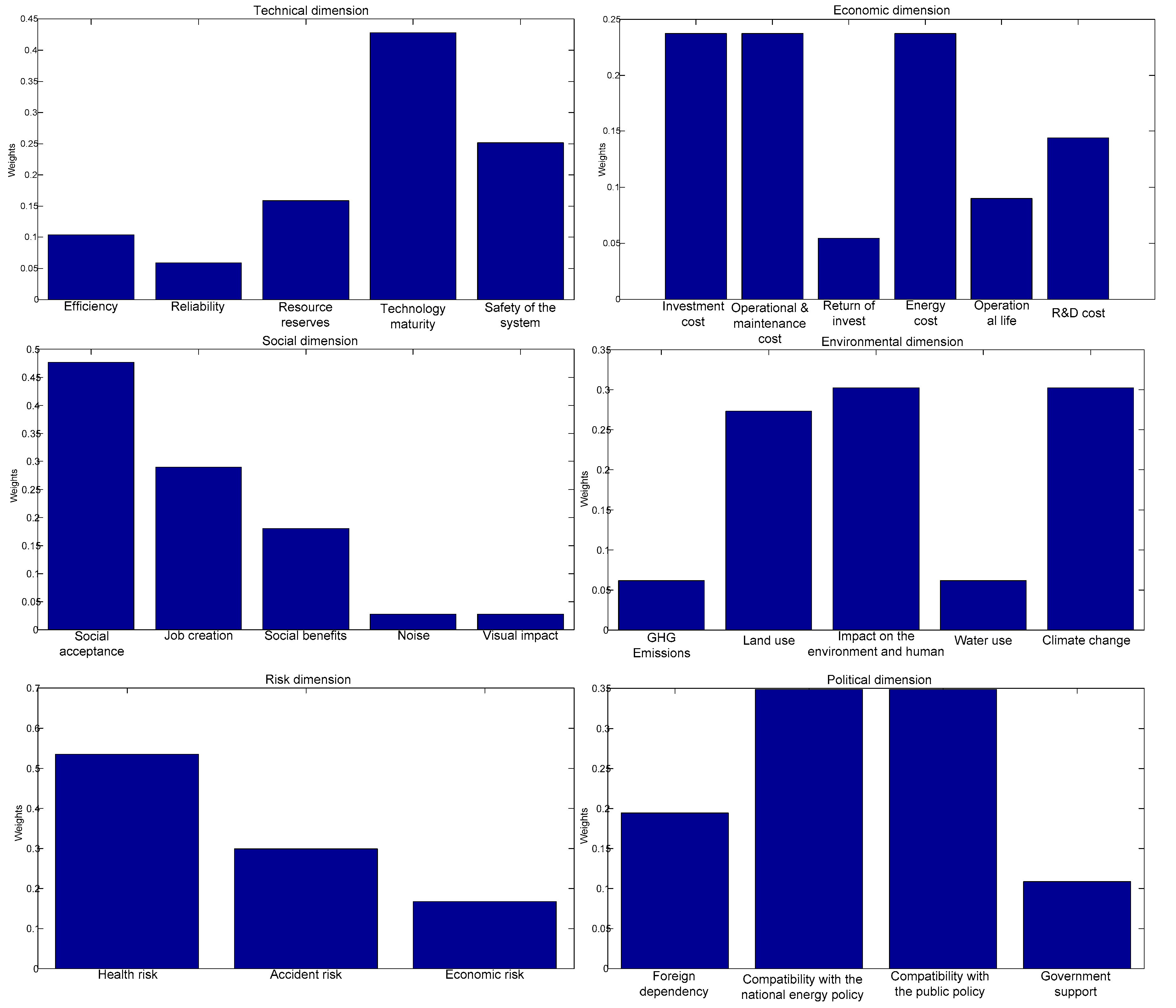
Table 3 enables us to note that in some M-BO and M-OW vectors, there are several best and worst criteria. So, based on the M-BO and M-OW dimensions, we notice the existence of one best criterion (Environmental—C4), whereas there are two worst criteria (Risk—C5 and Political—C6). In the Economic Sub-Criteria group, there are three best criteria (Investment cost—C21, Operation and maintenance cost—C22, and Energy cost—C24) and one worst criterion (Return of investment—C23). In the Social Sub-Criteria group, there is one best criterion (Social acceptance—C31) and two worst criteria (Noise—C34 and Visual impact—C35). The Environmental Sub-Criteria group is characteristic, since it contains two best criteria (Impact on the environment and humans—C43 and Climate change—C45) and two worst criteria (GHG Emissions—C41 and Water use—C44). In the Political Sub-Criteria group, there are two best criteria (Compatibility with the national energy policy—C62 and Compatibility with the public policy—C63) and one worst criterion (Government support—C64). In the remaining sub-criteria groups (the Technical Sub-Criteria and the Risk Sub-Criteria), there are the unique best and worst criteria, for which reason the traditional postulate of the BWM is used to define the weight coefficients of these sub-criteria groups.
Based on the M-BO and M-OW vectors (Table 3), the optimization models for the calculation of the weight coefficients of the dimensions/sub-criteria were defined. A total of seven BWM-I models were defined, some of which are shown in the next part.
By solving the presented models, the optimal values of the weight coefficients of the dimensions/sub-criteria are obtained, as shown in Table 4.
In Table 4, the global and local values of the weight coefficients of the criteria are presented. The global weights of the criteria were obtained by multiplying the weight coefficient of the dimension with the weight coefficients of the sub-criterion. By solving model (6), the values of , which are , , , , , , and were obtained. The values of are used to determine the consistency ratio, as shown in Table 5.
The analysis of the results of the BWM-I from Table 5 allows us to conclude that the values of the consistency ratio are satisfactory [27].
According to the findings shown in Table 4, the environmental dimension is determined to be the most crucial dimension, with the significance of 0.3972, only to be followed by the economic and technical dimensions, with the comparative weights of 0.2823 and 0.1674, respectively. According to Figure 1, in the pairwise comparison of the evaluation criteria, both “Impact on the environment and humans” and “Climate change” ranked as the priority factor from the environmental aspect, only to be followed by “Land use”. Furthermore, the three criteria (Investment cost, Operation and maintenance cost, and Energy cost) ranked the first in the ranking related to the economic dimension. “Technology maturity” and “social acceptance” were the most important criteria in terms of technological and social dimensions, respectively. Overall, according to the global weights, the most important criteria were “Climate change” (0.1199), “Impact on the environment and humans” (0.1199), “Land use” (0.1084), and “Technology maturity” (0.0716), indicating that the Climate change, Impact on the environment and humans, Land use, and Technology maturity criteria represent the four most crucial evaluation criteria for the determination of a suitable renewable energy source.
In order to show the sensitivity analysis of the BWM-I model, in the next section, we simulated the changes in the input parameters of the BO and OW vectors. In each group of criteria, another best or worst criterion was added, while the values of the remaining criteria in BO and OW vectors remained unchanged.
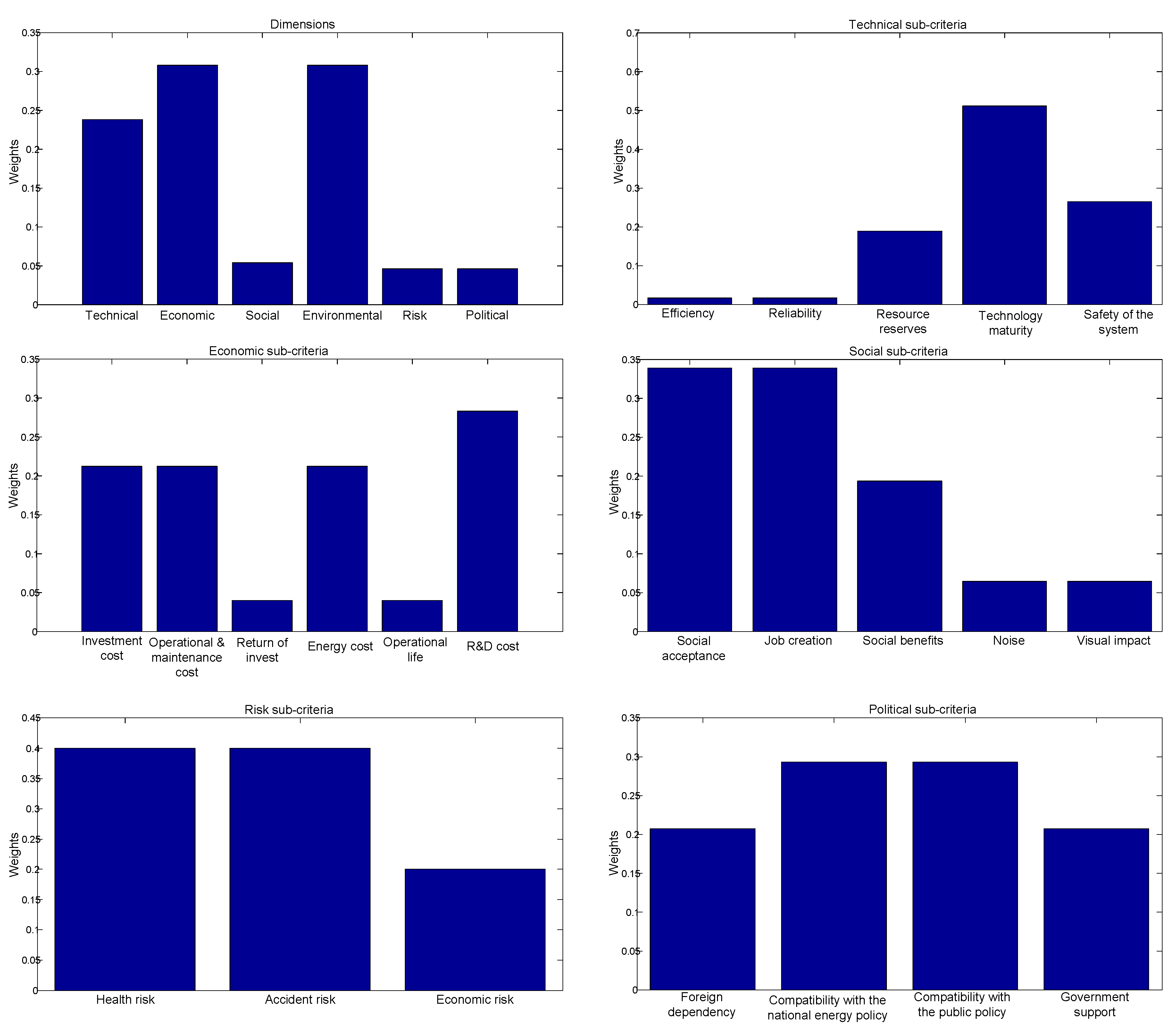
In the Dimensions group, two best criteria were selected (C4 and C2), while the remaining values of the criteria remained unchanged. In the Technical Sub-Criteria group, two criteria—C12 and C11—were selected as the worst criteria. In the Economic Sub-Criteria group, in addition to the three best criteria, the two worst criteria were selected (C23 and C25). In the Social Sub-Criteria group, two best criteria, C31 and C32, were added to the input BO and OW vectors. In the Risk Sub-Criteria group, in addition to the best criterion C51 and criterion C52, it was selected as the best criterion. In the Political Sub-Criteria group, in addition to C64, criterion C61 was also chosen as the worst criterion. After the implementation of these changes, the results shown in Figure 2 were obtained.
By analyzing the results from Figure 2, we notice that the model is sensitive to changes in the number of best and worst criteria in the input data. Despite the changes in the input data, the degree of consistency of the considered models remained within acceptable limits. The authors believe that the presented analysis shows the stability and robustness of the modified BWM methodology.
5. Managerial Implications
Integrating some methods into decision-making methodologies will make a significant contribution to the particular body of knowledge. Furthermore, it is valuable that the existing methods are made more efficient by completing their deficiencies. In decision theory, MCDM methods are utilized to solve many real-world problems. Improvement and development of the functionless side of an existing approach is always appreciated to continuously improve this branch of operations research, because businesses, politicians, researchers, and industries need such arrangements to make more reliable decisions.
The aim of this paper is pertinent to the fact that the BWM method, which is one of the new approaches in the field of MCDM, is ineffective if there is more than one best/worst criterion. Thus, this work suggests a novel strategy to solve an MCDM problem via some specific modifications to the main structure of the traditional BWM method. As a result, decision-makers will be able to easily cope with the problem of more than one best/worst criteria often encountered in real-world problems. Furthermore, by making fewer pairwise comparisons (only 2n-5), they will not only have to deal with the problem of inconsistency but also save time. Therefore, it is as well believed that the present article will give a different point of view for future works.
The presented methodology eliminates deviations in expert preferences that occur as a consequence of adapting to the traditional BWM algorithm. The previous analysis showed apparent advantages, so it is expected that the proposed methodology will be accepted by the management when solving real-world problems. Most decision-makers readily accept tools that are logical and easy to understand. The BWM-I methodology can be included in the category of easy-to-understand decision-making tools. In particular, it is expected to be accepted and used by decision-makers who know the algorithm of the traditional BWM, as well as its advantages and disadvantages. In addition, the use of the BWM-I methodology as part of the set of tools that make up the decision support system will make it more acceptable to management structures. This tool will be acceptable for managers who require a more realistic view of the mutual relations between the criteria, as well as a realistic and rational view of expert preferences.
A few insights are extracted to increase the applicability of the proposed BWM-I methodology in real cases. Thereby, the implications are as follows:
- By preferring the BWM-I model, authorities can make more accurate decisions.
- Since the weight of each criterion is found according to the opinions of decision-makers, firms can improve their evaluation process through the BWM-I approach.
- Firms can create a better competitive advantage over their business competitors by determining the best alternatives with the BWM-I model.
Knowing that the decision-making process is accompanied by greater or lesser uncertainties caused by a dynamic environment, such a system eliminates further adjustment and deviation of expert preferences. As a result of this feature, the demonstrated methodology can help companies establish a rational, systematic approach to evaluating the internal and external factors that affect their business. The flexibility of the methodology in terms of reducing the number of pairwise comparisons is also valuable. It is expected that the flexibility of the BWM-I methodology will enable its application in complex studies in which criteria and expert preferences differ and in which no consensus is required in expert preferences.
6. Conclusions
The BWM method represents a very powerful tool for multi-criteria decision-making and defining criteria weight coefficients. Generally viewed, while solving real-world problems, there are specific multi-criteria problems in which there are several criteria with the same influence on decision-making. The traditional postulate of the BWM implies that while defining priority vectors (BO and OW), one best criterion and one worst criterion should be chosen from within a set of the observed criteria. Then, the criteria are compared in pairs by defining the best-to-others (BO) and others-to-worst (OW) vectors. While defining the BO and OW vectors, the decision-maker may assign the same criteria preferences while comparing the BO and OW, which means that there may be several criteria with the same significance. However, the traditional BWM does not permit the defining of several best/worst criteria that will have the same significance, although it is frequently the case in real-world problems. As a result of that, by applying the traditional BWM, decision-makers are required to define one best/worst criterion should they believe that there are two or more best/worst criteria. In that way, the decision-maker’s preferences are distorted to a certain extent, and no objective results are obtained. Should the small flexibility of the 9-degree scale be added to that as well, then the obtained values of criteria weights may significantly deviate from the preferences expressed by the decision-maker.
In this paper, the improvement of the traditional BWM is presented. The improved BWM (BWM-I) eliminates the shortcomings of the traditional BWM. It offers a possibility for decision-makers to express their preferences even in the cases when there is more than one best and worst criterion. The BWM-I was successfully tested on two examples in this paper. In the first example in Section 3, a case in which there are two best criteria is presented. The algorithm of the traditional BWM and the BWM-I was also applied to the same example. It was shown that the BWM-I has greater flexibility in expressing experts’ preferences in relation to the traditional BWM. In the second example (Section 4), the BWM-I was applied to the defining of the weight coefficients of the criteria in the field of renewable energy and their ranking. In the presented example, all of the 28 criteria grouped into the six dimensions were subjected to evaluation. Through a combination of the seven models of the BWM-I, the advantages of the developed model and the possibilities of the objective processing of experts’ preferences are demonstrated.
In comparison with the traditional BWM, the proposed BWM-I has several advantages according to the following:
- (1)
- Due to non-determinedness and imprecision in data, it is realistic that more than one best and/or worst criterion/criteria with the same significance may appear in experts’ preferences. The BWM-I enables a realistic expression of experts’ preferences irrespective of the number of the best/worst criteria in a set of evaluation criteria.
- (2)
- In case more than one best and worst criterion appear ( and ) in the decision-making process, the application of the BWM-I reduces the number of comparisons from 2n-3 (in the traditional BWM) to 2n-5 (in the BWM-I). In that manner, the possibility of making a mistake while conducting a pairwise comparison of the criteria is also reduced, which further exerts an influence on the greater reliability of results.
- (3)
- The flexibility of the BWM-I is expressed in two ways: (1) the possibilities of the realistic processing of experts’ preferences irrespective of the number of the criteria with the same significance (even in the case of the best/worst criteria), and (2) in the case of , the BWM-I transforms into the traditional BWM. This flexibility opens the possibility of applying the BWM-I in complex studies, in which criteria and experts’ preferences differ within the framework of the cluster(s)/group of criteria.
Future Research
The proposed BWM-I represents a tool that is capable of being successfully integrated with other MCDM techniques. The development of the hybrid multi-criteria models for group decision-making that would be based on the integration of the BWM-I into other MCDM tools represents one of the future directions of its application. The second logical step for the future improvement of the BWM-I is its application in an uncertain environment, such as fuzzy, rough, grey, neutrosophic, and so on [67,68]. In the last few years, numerous linguistic approaches, such as the expansions of linguistic variables in a neutrosophic environment and the unbalanced linguistic approach, have been developed. The mentioned approaches have attracted considerable attention to the decision-making field through the possibility of applying linguistic variables in the decision-making process. Connecting these linguistic approaches with the BWM-I and research into the possibility of the linguistic modeling of preferences are interesting and promising topics in future research.
Author Contributions
Conceptualization, methodology, validation, D.P. and F.E.; writing—original draft preparation, review and editing, D.P., F.E., G.C. and M.A.A. All authors have read and agreed to the published version of the manuscript.
Funding
This research received no external funding.
Conflicts of Interest
The authors declare no conflict of interest.
References
- Stankovic, M.; Gladovic, P.; Popovic, V. Determining the importance of the criteria of traffic accessibility using fuzzy AHP and rough AHP method. Decis. Mak. Appl. Manag. Eng. 2019, 2, 86–104. [Google Scholar] [CrossRef]
- Petrovic, G.; Mihajlovic, J.; Cojbasic, Z.; Madic, M.; Marinkovic, D. Comparison of three fuzzy MCDM methods for solving the supplier selection problem. Facta Univ. Ser. Mech. Eng. 2019, 17, 455–469. [Google Scholar] [CrossRef]
- Hassanpour, M. Evaluation of Iranian Wood and Cellulose Industries. Decis. Mak. Appl. Manag. Eng. 2019, 2, 13–34. [Google Scholar] [CrossRef]
- Diyaley, S.; Chakraborty, S. Optimization of multi-pass face milling parameters using metaheuristic algorithms. Facta Univ. Ser. Mech. Eng. 2019, 17, 365–383. [Google Scholar] [CrossRef]
- Tzeng, G.-H.; Chen, T.-Y.; Wang, J.C. A weight-assessing method with habitual domains. Eur. J. Oper. Res. 1998, 110, 342–367. [Google Scholar] [CrossRef]
- Shannon, C.E.; Weaver, W. The Mathematical Theory of Communication; The University of Illinois Press: Urbana, IL, USA, 1947. [Google Scholar]
- Diakoulaki, D.; Mavrotas, G.; Papayannakis, L. Determining objective weights in multiple criteria problems: The CRITIC method. Comput. Oper. Res. 1995, 22, 763–770. [Google Scholar] [CrossRef]
- Srdjevic, B.; Medeiros, Y.D.P.; Faria, A.S.; Schaer, M. Objektivno vrednovanje kriterijuma performanse sistema akumulacija. Vodoprivreda 2003, 35, 163–176. (In Serbian) [Google Scholar]
- Thurstone, L.L. A law of comparative judgment. Psychol. Rev. 1927, 34, 273. [Google Scholar] [CrossRef]
- Saaty, T.L. Analytic Hierarchy Process; McGraw-Hill: New York, NY, USA, 1980. [Google Scholar]
- Rezaei, J. Best-worst multi-criteria decision-making method. Omega 2015, 53, 49–57. [Google Scholar] [CrossRef]
- Hashemkhani Zolfani, S.; Yazdani, M.; Zavadskas, E.K. An extended stepwise weight assessment ratio analysis (SWARA) method for improving criteria prioritization process. Soft Comput. 2018, 22, 7399–7405. [Google Scholar] [CrossRef]
- Ecer, F. An integrated Fuzzy AHP and ARAS model to evaluate mobile banking services. Technol. Econ. Dev. Econ. 2018, 24, 670–695. [Google Scholar] [CrossRef] [Green Version]
- Ecer, F. Multi-criteria decision making for green supplier selection using interval type-2 fuzzy AHP: A case study of a home appliance manufacturer. Oper. Res. 2020, 1–35. [Google Scholar] [CrossRef]
- Badi, I.; Abdulshahed, A. Ranking the Libyan airlines by using full consistency method (FUCOM) and analytical hierarchy process (AHP). Oper. Res. Eng. Sci. Theory Appl. 2019, 2, 1–14. [Google Scholar] [CrossRef] [Green Version]
- Pamučar, D.; Lukovac, V.; Božanić, D.; Komazec, N. Multi-criteria FUCOM-MAIRCA model for the evaluation of level crossings: Case study in the Republic of Serbia. Oper. Res. Eng. Sci. Theory Appl. 2018, 1, 108–129. [Google Scholar] [CrossRef]
- Durmic, E.; Stevic, Z.; Chatterjee, P.; Vasiljevic, M.; Tomasevic, M. Sustainable supplier selection using combined FUCOM—Rough SAW model. Rep. Mech. Eng. 2020, 1, 34–43. [Google Scholar] [CrossRef]
- Rostamzadeh, R.; Ghorabaee, M.K.; Govindan, K.; Esmaeili, A.; Nobar, H.B.K. Evaluation of sustainable supply chain risk management using an integrated fuzzy TOPSIS-CRITIC approach. J. Clean. Prod. 2018, 175, 651–669. [Google Scholar] [CrossRef]
- Ecer, F. A Multi-criteria Approach Towards Assessing Corporate Sustainability Performances of Privately-owned Banks: Entropy-ARAS Integrated Model. Eskişehir Osman. Univ. J. Econ. Adm. Sci. 2019, 14, 365–390. [Google Scholar]
- Zizovic, M.; Pamucar, D. New model for determining criteria weights: Level Based Weight Assessment (LBWA) model. Decis. Mak. Appl. Manag. Eng. 2019, 2, 1–12. [Google Scholar] [CrossRef]
- Van de Kaa, G.; Fens, T.; Rezaei, J.; Kaynak, D.; Hatun, Z.; Tsilimeni-Archangelidi, A. Realizing smart meter connectivity: Analyzing the competing technologies Power line communication, mobile telephony, and radio frequency using the best worst method. Renew. Sustain. Energy Rev. 2019, 103, 320–327. [Google Scholar] [CrossRef]
- Setyono, R.P.; Sarno, R. Vendor Track Record Selection Using Best Worst Method. In Proceedings of the 2018 International Seminar on Application for Technology of Information and Communication, Semarang, Indonesia, 7 October 2018; pp. 41–48. [Google Scholar]
- Ahmadi, H.; Ku Kusi-Sarpong, S.; Rezaei, J. Assessing the social sustainability of supply chains using Best Worst Method. Recourses Conserv. Recycl. 2017, 126, 99–106. [Google Scholar] [CrossRef]
- Salimi, N.; Rezaei, J. Evaluating firms’ R&D performance using best worst method. Eval. Program Plan. 2018, 66, 147–155. [Google Scholar]
- Beemsterboer, D.J.C.; Hendrix, E.M.T.; Claassen, G.D.H. On solving the Best-Worst Method in multi-criteria decision-making. IFAC-PapersOnLine 2018, 51, 1660–1665. [Google Scholar] [CrossRef]
- Rezaei, J.; Wang, J.; Tavasszy, L. Linking supplier development to supplier segmentation using Best Worst Method. Expert Syst. Appl. 2015, 42, 9152–9164. [Google Scholar] [CrossRef]
- Rezaei, J. Best-worst multi-criteria decision-making method: Some properties and a linear model. Omega 2016, 64, 126–130. [Google Scholar] [CrossRef]
- Ghaffari, S.; Arab, A.; Nafari, J.; Manteghi, M. Investigation and evaluation of key success factors in technological innovation development based on BWM. Decis. Sci. Lett. 2017, 6, 295–306. [Google Scholar] [CrossRef]
- Gupta, P.; Anand, S.; Gupta, H. Developing a roadmap to overcome barriers to energy efficiency in buildings using best worst method. Sustain. Cities Soc. 2017, 31, 244–259. [Google Scholar] [CrossRef]
- Praditya, D.; Janssen, M. Assessment of factors influencing information sharing arrangements using the best-worst method. In Proceedings of the Conference on e-Business, e-Services and e-Society, Dlehi, India, 21 November 2017; Springer: Cham, Switzerland; pp. 94–106. [Google Scholar]
- Yadollahi, S.; Kazemi, A.; Ranjbarian, B. Identifying and prioritizing the factors of service experience in banks: A Best-Worst method. Decis. Sci. Lett. 2018, 7, 455–464. [Google Scholar] [CrossRef]
- Kheybari, S.; Kazemi, M.; Rezaei, J. Bioethanol facility location selection using best-worst method. Appl. Energy 2019, 242, 612–623. [Google Scholar] [CrossRef]
- Raj, A.; Srivastava, S.K. Sustainability performance assessment of an aircraft manufacturing firm. Benchmark. Int. J. 2018, 25, 1500–1527. [Google Scholar] [CrossRef]
- Torbati, A.R.; Sayadi, M.K. A New Approach to Investigate the Performance of Insurance Branches in Iran Using Best-Worst Method and Fuzzy Inference System. J. Soft Comput. Decis. Support Syst. 2018, 5, 13–18. [Google Scholar]
- Khanmohammadi, E.; Zandieh, M.; Tayebi, T. Drawing a Strategy Canvas Using the Fuzzy Best–Worst Method. Glob. J. Flex. Syst. Manag. 2019, 20, 57–75. [Google Scholar] [CrossRef]
- Gupta, H.; Barua, M.K. A framework to overcome barriers to green innovation in SMEs using BWM and Fuzzy TOPSIS. Sci. Total Environ. 2018, 633, 122–139. [Google Scholar] [CrossRef] [PubMed]
- You, P.; Guo, S.; Zhao, H.; Zhao, H. Operation performance evaluation of power grid enterprise using a hybrid BWM-TOPSIS method. Sustainability 2017, 9, 2329. [Google Scholar] [CrossRef] [Green Version]
- Askarifar, K.; Motaffef, Z.; Aazaami, S. An investment development framework in Iran’s seashores using TOPSIS and best-worst multi-criteria decision making methods. Decis. Sci. Lett. 2018, 7, 55–64. [Google Scholar] [CrossRef]
- Garg, C.P.; Sharma, A. Sustainable outsourcing partner selection and evaluation using an integrated BWM–VIKOR framework. Environ. Dev. Sustain. 2018, 1–29. [Google Scholar] [CrossRef]
- Cheraghalipour, A.; Paydar, M.M.; Hajiaghaei-Keshteli, M. Applying a hybrid BWM-VIKOR approach to supplier selection: A case study in the Iranian agricultural implements industry. Int. J. Appl. Decis. Sci. 2018, 11, 274–301. [Google Scholar] [CrossRef]
- Kumar, A.; Aswin, A.; Gupta, H. Evaluating green performance of the airports using hybrid BWM and VIKOR methodology. Tour. Manag. 2020, 76, 103941. [Google Scholar] [CrossRef]
- Yucesan, M.; Mete, S.; Serin, F.; Celik, E.; Gul, M. An integrated best-worst and interval type-2 fuzzy TOPSIS methodology for green supplier selection. Mathematics 2019, 7, 182. [Google Scholar] [CrossRef] [Green Version]
- Pamučar, D.; Gigović, L.; Bajić, Z.; Janošević, M. Location selection for wind farms using GIS multi-criteria hybrid model: An approach based on fuzzy and rough numbers. Sustainability 2017, 9, 1315. [Google Scholar] [CrossRef] [Green Version]
- Stević, Ž.; Pamučar, D.; Kazimieras Zavadskas, E.; Ćirović, G.; Prentkovskis, O. The selection of wagons for the internal transport of a logistics company: A novel approach based on rough BWM and rough SAW methods. Symmetry 2017, 9, 264. [Google Scholar] [CrossRef] [Green Version]
- Alimohammadlou, M.; Bonyani, A. Fuzzy BWANP multi-criteria decision-making method. Decis. Sci. Lett. 2019, 8, 85–94. [Google Scholar] [CrossRef]
- Amoozad Mahdiraji, H.; Arzaghi, S.; Stauskis, G.; Zavadskas, E. A hybrid fuzzy BWM-COPRAS method for analyzing key factors of sustainable architecture. Sustainability 2018, 10, 1626. [Google Scholar] [CrossRef] [Green Version]
- Bonyani, A.; Alimohammadlou, M. Identifying and prioritizing foreign companies interested in participating in post-sanctions Iranian energy sector. Energy Strategy Rev. 2018, 21, 180–190. [Google Scholar] [CrossRef]
- Pamučar, D.; Chatterjee, K.; Zavadskas, E.K. Assessment of third-party logistics provider using multi-criteria decision-making approach based on interval rough numbers. Comput. Ind. Eng. 2019, 127, 383–407. [Google Scholar] [CrossRef]
- Sofuoglu, M.A.; Orak, S. A novel hybrid multi criteria decision making model: Application to turning operations. Int. J. Intell. Syst. Appl. Eng. 2017, 5, 124–131. [Google Scholar] [CrossRef] [Green Version]
- Serrai, W.; Abdelli, A.; Mokdad, L.; Hammal, Y. Towards an efficient and a more accurate web service selection using MCDM methods. J. Comput. Sci. 2017, 22, 253–267. [Google Scholar] [CrossRef]
- Hashemkhani Zolfani, S.; Pamucar, D.; Ecer, F.; Raslanas, S. Neighborhood Selection for a Newcomer via a Novel BWM-Based Revised MAIRCA Integrated Model; a Case from the Coquimbo-La Serena Conurbation, Chile. Int. J. Strateg. Prop. Manag. 2020, 24, 102–118. [Google Scholar] [CrossRef]
- Ergu, D.; Kou, G.; Peng, Y.; Shi, Y. A simple method to improve the consistency ratio of the pair-wise comparison matrix in ANP. Eur. J. Oper. Res. 2013, 213, 246–259. [Google Scholar] [CrossRef]
- Anane, M.; Kallali, H.; Jellali, S.; Ouessar, M. Ranking suitable sites for Soil Aquifer Treatment in Jerba Island (Tunisia) using remote sensing, GIS and AHP-multicriteria decision analysis. Int. J. Water 2008, 4, 121–135. [Google Scholar] [CrossRef]
- Ishizaka, A. Comparison of Fuzzy logic, AHP, FAHP and Hybrid Fuzzy AHP for new supplier selection and its performance analysis. Int. J. Integr. Supply Manag. 2014, 9, 1–22. [Google Scholar] [CrossRef] [Green Version]
- Pamucar, D.; Bozanic, D.; Lukovac, V.; Komazec, N. Normalized weighted geometric Bonferroni mean operator of interval rough numbers—Application in interval rough DEMATEL-COPRAS. Facta Univ. Ser. Mech. Eng. 2018, 16, 171–191. [Google Scholar] [CrossRef]
- Haddad, B.; Liazid, A.; Ferreira, P. A multi-criteria approach to rank renewables for the Algerian electricity system. Renew. Energy 2017, 107, 462–472. [Google Scholar] [CrossRef]
- Yilan, G.; Kadirgan, M.N.; Çiftçioğlu, G.A. Analysis of electricity generation options for sustainable energy decision making: The case of Turkey. Renew. Energy 2020, 146, 519–529. [Google Scholar] [CrossRef]
- Büyüközkan, G.; Güleryüz, S. Evaluation of Renewable Energy Resources in Turkey using an integrated MCDM approach with linguistic interval fuzzy preference relations. Energy 2017, 123, 149–163. [Google Scholar] [CrossRef]
- Çelikbilek, Y.; Tüysüz, F. An integrated grey based multi-criteria decision making approach for the evaluation of renewable energy sources. Energy 2016, 115, 1246–1258. [Google Scholar] [CrossRef]
- Cavallaro, F.; Zavadskas, E.K.; Streimikiene, D.; Mardani, A. Assessment of concentrated solar power (CSP) technologies based on a modified intuitionistic fuzzy TOPSIS and trigonometric entropy weights. Technol. Forecast. Soc. Chang. 2019, 140, 258–270. [Google Scholar] [CrossRef]
- Malkawi, S.; Azizi, D. A multi-criteria optimization analysis for Jordan’s energy mix. Energy 2017, 127, 680–696. [Google Scholar] [CrossRef]
- Cartelle Barros, J.; Coira, M.L.; De la Cruz López, M.P.; del Caño Gochi, A. Assessing the global sustainability of different electricity generation systems. Energy 2015, 89, 473–489. [Google Scholar] [CrossRef]
- Troldborg, M.; Heslop, S.; Hough, R.L. Assessing the sustainability of renewable energy technologies using multi-criteria analysis: Suitability of approach for national-scale assessments and associated uncertainties. Renew. Sustain. Energy Rev. 2014, 39, 1173–1184. [Google Scholar] [CrossRef]
- Büyüközkan, G.; Karabulut, Y.; Mukul, E. A novel renewable energy selection model for United Nations’ sustainable development goals. Energy 2018, 165, 290–302. [Google Scholar] [CrossRef]
- Büyüközkan, G.; Güleryüz, S. An integrated DEMATEL-ANP approach for renewable energy resources selection in Turkey. Int. J. Prod. Econ. 2016, 182, 435–448. [Google Scholar] [CrossRef]
- Wang, J.J.; Jing, Y.Y.; Zhang, C.F.; Zhao, J.H. Review on multi-criteria decision analysis aid in sustainable energy decision-making. Renew. Sustain. Energy Rev. 2009, 13, 2263–2278. [Google Scholar] [CrossRef]
- Pamucar, D. Normalized Weighted Geometric Dombi Bonferoni Mean Operator with Interval Grey Numbers: Application in Multicriteria Decision Making. Rep. Mech. Eng. 2020, 1, 44–52. [Google Scholar] [CrossRef]
- Li, J.; Wang, J.Q.; Hu, J.H. Multi-criteria decision-making method based on dominance degree and BWM with probabilistic hesitant fuzzy information. Int. J. Mach. Learn. Cybern. 2019, 10, 1671–1685. [Google Scholar]
Figure 1.
The local weights of the criteria according to the considered dimensions.

Figure 2.
Results of modified M-BO and M-OW vectors of the dimensions/sub-criteria.


Table 1.
The best-to-others and others-to-worst pairwise comparison vectors.
| Best-to-Others Vector | Others-to-Worst Vector | ||
|---|---|---|---|
| Best: C2 and C4 | Evaluation | Worst: C5 | Evaluation |
| C1 | 2 | C1 | 4 |
| C2 | 1 | C2 | 9 |
| C3 | 4 | C3 | 2 |
| C4 | 1 | C4 | 9 |
| C5 | 9 | C5 | 1 |
Table 2.
The criteria and sub-criteria used in this paper.
| Main Criteria | Sub-Criteria | Code | Definition | References |
|---|---|---|---|---|
| Technical (C1) | Efficiency | C11 | How technology is widespread at the regional, national, and international levels. | [57,58,59] |
| Reliability | C12 | An energy system’s ability to perform the required functions | [56,58,60] | |
| Resource reserves | C13 | The availability of the energy source to generate energy | [58] | |
| Technology maturity | C14 | The penetration of a specific technology in the
energy mix at the regional, national, and international levels. | [58,60] | |
| Safety of the system | C15 | The security of the workers and the local community | [56] | |
| Economic (C2) | Investment cost | C21 | All costs of products and services, except for the costs of labor or the cost of equipment maintenance | [56,58,59,60] |
| Operation and maintenance cost | C22 | Operating the energy system adequately, as well as the costs related to the maintenance of the energy system | [56,58] | |
| Return of investment | C23 | The time required to recover the investment | [56,58] | |
| Energy cost | C24 | The cost of the energy-generating system | [60,63] | |
| Operational life | C25 | The period during which the power plant can operate before being decommissioned | [56] | |
| R&D cost | C26 | The expenses incurred for the R&D of technological innovations | [65] | |
| Social (C3) | Social acceptance | C31 | The opinions of residents, local authorities, and other stakeholders on an energy project | [56,57,58] |
| Job creation | C32 | Jobs created per unit of the energy produced | [57,58,61] | |
| Social benefits | C33 | The contribution of an energy system to the improvement and advancement of local society | [56,58] | |
| Noise | C34 | The noise generated during the lifecycle under
consideration | [62] | |
| Visual impact | C35 | The aesthetics of the installations of the energy system | [62] | |
| Environmental (C4) | Greenhouse Gas (GHG) Emissions | C41 | Lifecycle GHG emissions (in the equivalent emission of CO2) from technology | [58,61,63] |
| Land use | C42 | The area used per unit of the energy produced | [58,59,60,61] | |
| Impact on the environment and humans | C43 | The detriment level of the energy facility to humans and nature | [58,59,60,64] | |
| Water use | C44 | Water consumed per unit of the energy produced | [60,61] | |
| Climate change | C45 | The global warming potential | [57] | |
| Risk (C5) | Health risk | C51 | Emissions harmful to human health | [66] |
| Accident risk | C52 | Accidents of any type during the lifecycle considered | [57,59,62,66] | |
| Economic risk | C53 | The risk financial stakeholders should bear for business in new plants | [60] | |
| Political (C6) | Foreign dependency | C61 | The dependency of countries on international legislations | [57,58] |
| Compatibility with the national energy policy | C62 | The national energy policy related to renewable energy sources | [58] | |
| Compatibility with the public policy | C63 | Voluntary agreements and general codes of conduct in line with national priorities | [64] | |
| Government support | C64 | Approving and adapting to renewable energy sources. | [64] |
Table 3.
The best-to-others (M-BO) and modified others-to-worst (M-OW) vectors of the dimensions/sub-criteria.
Table 3.
The best-to-others (M-BO) and modified others-to-worst (M-OW) vectors of the dimensions/sub-criteria.
| Dimensions | |||
| Best: C4 | Preference | Worst: C5 and C6 | Preference |
| C1 | 3 | C1 | 3 |
| C2 | 2 | C2 | 4 |
| C3 | 4 | C3 | 2 |
| C4 | 1 | C4 | 5 |
| C5 | 5 | C5 | 1 |
| C6 | 5 | C6 | 1 |
| Technical sub-criteria | |||
| Best: C14 | Preference | Worst: C12 | Preference |
| C11 | 4 | C11 | 2 |
| C12 | 7 | C12 | 1 |
| C13 | 3 | C13 | 3 |
| C14 | 1 | C14 | 7 |
| C15 | 2 | C15 | 4 |
| Economic sub-criteria | |||
| Best: C21, C22 and C24 | Preference | Worst: C23 | Preference |
| C21 | 1 | C21 | 4 |
| C22 | 1 | C22 | 4 |
| C23 | 4 | C23 | 1 |
| C24 | 1 | C24 | 4 |
| C25 | 3 | C25 | 2 |
| C26 | 2 | C26 | 3 |
| Social sub-criteria | |||
| Best: C31 | Preference | Worst: C34 and C35 | Preference |
| C31 | 1 | C31 | 4 |
| C32 | 2 | C32 | 3 |
| C33 | 3 | C33 | 2 |
| C34 | 4 | C34 | 1 |
| C35 | 4 | C35 | 1 |
| Environmental sub-criteria | |||
| Best: C43 and C45 | Preference | Worst: C41 and C44 | Preference |
| C41 | 4 | C41 | 1 |
| C42 | 2 | C42 | 2 |
| C43 | 1 | C43 | 4 |
| C44 | 4 | C44 | 1 |
| C45 | 1 | C45 | 4 |
| Risk sub-criteria | |||
| Best: C51 | Preference | Worst: C53 | Preference |
| C51 | 1 | C51 | 3 |
| C52 | 2 | C52 | 2 |
| C53 | 3 | C53 | 1 |
| Political sub-criteria | |||
| Best: C62 and C63 | Preference | Worst: C64 | Preference |
| C61 | 2 | C61 | 2 |
| C62 | 1 | C62 | 3 |
| C63 | 1 | C63 | 3 |
| C64 | 3 | C64 | 1 |
Table 4.
The optimal values of the weight coefficients of the dimensions/sub-criteria.
| Dimensions/Sub-Criteria | Code | Local Weights | Global Weights | Rank |
|---|---|---|---|---|
| Technical | C1 | 0.1674 | - | 3 |
| Efficiency | C11 | 0.1037 | 0.0174 | 17 |
| Reliability | C12 | 0.0586 | 0.0098 | 19 |
| Resource reserves | C13 | 0.1584 | 0.0265 | 12 |
| Technology maturity | C14 | 0.4278 | 0.0716 | 4 |
| Safety of the system | C15 | 0.2514 | 0.0421 | 9 |
| Economic | C2 | 0.2823 | - | 2 |
| Investment cost | C21 | 0.2372 | 0.0670 | 5 |
| Operation and maintenance cost | C22 | 0.2372 | 0.0670 | 5 |
| Return of investment | C23 | 0.0545 | 0.0154 | 18 |
| Energy cost | C24 | 0.2372 | 0.0670 | 5 |
| Operational life | C25 | 0.0897 | 0.0253 | 13 |
| R&D cost | C26 | 0.1441 | 0.0407 | 10 |
| Social | C3 | 0.1178 | - | 4 |
| Social acceptance | C31 | 0.4761 | 0.0561 | 8 |
| Job creation | C32 | 0.2893 | 0.0341 | 11 |
| Social benefits | C33 | 0.1799 | 0.0212 | 16 |
| Noise | C34 | 0.0273 | 0.0032 | 25 |
| Visual impact | C35 | 0.0273 | 0.0032 | 25 |
| Environmental | C4 | 0.3972 | - | 1 |
| GHG Emissions | C41 | 0.0617 | 0.0245 | 14 |
| Land use | C42 | 0.2729 | 0.1084 | 3 |
| Impact on the environment and humans | C43 | 0.3019 | 0.1199 | 1 |
| Water use | C44 | 0.0617 | 0.0245 | 14 |
| Climate change | C45 | 0.3019 | 0.1199 | 1 |
| Risk | C5 | 0.0176 | - | 5 |
| Health risk | C51 | 0.5348 | 0.0094 | 20 |
| Accident risk | C52 | 0.2985 | 0.0053 | 23 |
| Economic risk | C53 | 0.1667 | 0.0029 | 27 |
| Political | C6 | 0.0176 | - | 5 |
| Foreign dependency | C61 | 0.1945 | 0.0034 | 24 |
| Compatibility with the national energy policy | C62 | 0.3484 | 0.0061 | 21 |
| Compatibility with the public policy | C63 | 0.3484 | 0.0061 | 21 |
| Government support | C64 | 0.1086 | 0.0019 | 28 |
Table 5.
The consistency index and the consistency ratio of our modified Best Worst Method (BWM-I).
| Criterion Level | C1–C6 | C11–C15 | C21–C26 | C31–C35 | C41–C45 | C51–C53 | C61–C64 |
|---|---|---|---|---|---|---|---|
| 5 | 7 | 4 | 4 | 4 | 3 | 3 | |
| CI () | 2.30 | 3.73 | 1.63 | 1.63 | 1.63 | 1.00 | 1.00 |
| CR | 0.27 | 0.08 | 0.22 | 0.22 | 0.55 | 0.21 | 0.21 |
© 2020 by the authors. Licensee MDPI, Basel, Switzerland. This article is an open access article distributed under the terms and conditions of the Creative Commons Attribution (CC BY) license (http://creativecommons.org/licenses/by/4.0/).
Share and Cite
MDPI and ACS Style
Pamučar, D.; Ecer, F.; Cirovic, G.; Arlasheedi, M.A. Application of Improved Best Worst Method (BWM) in Real-World Problems. Mathematics 2020, 8, 1342. https://0-doi-org.brum.beds.ac.uk/10.3390/math8081342
AMA Style
Pamučar D, Ecer F, Cirovic G, Arlasheedi MA. Application of Improved Best Worst Method (BWM) in Real-World Problems. Mathematics. 2020; 8(8):1342. https://0-doi-org.brum.beds.ac.uk/10.3390/math8081342
Chicago/Turabian StylePamučar, Dragan, Fatih Ecer, Goran Cirovic, and Melfi A. Arlasheedi. 2020. "Application of Improved Best Worst Method (BWM) in Real-World Problems" Mathematics 8, no. 8: 1342. https://0-doi-org.brum.beds.ac.uk/10.3390/math8081342
Note that from the first issue of 2016, this journal uses article numbers instead of page numbers. See further details here.