Explicit Continuity Conditions for G¹ Connection of S-λ Curves and Surfaces

Abstract

The S-λ model is one of the most useful tools for shape designs and geometric representations in computer-aided geometric design (CAGD), which is due to its good geometric properties such as symmetry, shape adjustable property. With the aim to solve the problem that complex S-λ curves and surfaces cannot be constructed by a single curve and surface, the explicit continuity conditions for G¹ connection of S-λ curves and surfaces are investigated in this paper. On the basis of linear independence and terminal properties of S-λ basis functions, the conditions of G¹ geometric continuity between two adjacent S-λ curves and surfaces are proposed, respectively. Modeling examples imply that the continuity conditions proposed in this paper are easy and effective, which indicate that the S-λ curves and surfaces can be used as a powerful supplement of complex curves and surfaces design in computer aided design/computer aided manufacturing (CAD/CAM) system.

1. Introduction

In the design of complex curves and surfaces, the basis functions of geometric models determine the properties of the curves and surfaces constructed. The basis functions of common models in CAGD include the Bernstein basis function, the Poisson basis function, the negative Bernstein basis function, the B-spline basis function and so on, which are closely related to the probability distribution—especially the discrete probability distribution [1,2]. For example, the Bernstein basis function contained in the Bézier model is taken from binomial distribution, and the B-spline basis function used in the B-spline model is closely related to some stochastic processes [3]. The negative Bernstein basis function which was proposed by Goldman [4] corresponds to the negative binomial distribution, and the Poisson basis function advanced by Goldman and Morin [5] corresponds to the Poisson distribution. The S-λ basis functions proposed by [6,7] are a kind of discrete probability modeling defined by generating function and transformation factor combined with probability convolution. By taking different generating functions and transformation factors, different S-λ basis functions can be obtained, such as the Bernstein basis function, the Poisson basis function, the negative Bernstein basis function, etc. Therefore, we can study these well-known basis functions mentioned above in a unified way by S-λ basis function. Furthermore, S-λ curves and surfaces include Bézier curves and surfaces, Poisson curves and surfaces, rational Bézier curves and surfaces as well as many other curves and surfaces. In conclusion, the studies of S-λ methods provide a unified scheme for dealing with these curves and surfaces and reveal the relations among these curves and surfaces. Consequently, the related studies based on the S-λ curves and surfaces have great significant value in theory and practical application. Based on the advantages of the S-λ model, Lu and Qin [8] proposed a degree reduction method of S-λ curves on the basis of genetic simulated annealing algorithm. Chen et al. [9] proposed a new shape-adjustment method of S-λ curves. Some applications of S-λ model can be found in [10,11].

In addition, in the geometric-modeling design of CAD/CAM, a problem often encountered is that complex curves and surfaces cannot be constructed by a single curve and surface. Hence, it is necessary to study the geometric continuity conditions for S-λ curves and surfaces. To date, there are two kinds of methods established for the continuity between geometric models [12]. One is parametric continuity, which is called Cⁿ continuity. The other is geometric continuity, or Gⁿ continuity. Furthermore, it is usually required to satisfy some certain conditions. For example, for two adjacent parametric curves P(t) and Q(t), the necessary and sufficient conditions for G¹ smooth continuity are P(1) = Q(0) and P’(1) = αQ’(0), where $\alpha >0$ is a constant. Similarly, if two surfaces need to satisfy G¹ continuity, they should not only have a common boundary curve, but also have a common tangent plane at the common joint. In order to solve the problem mentioned above, many international scholars have done many studies on the related algorithms of geometric continuity conditions for different geometric models [13,14,15,16,17,18,19,20,21,22,23,24,25,26,27,28,29,30].

As we all know, the geometric continuity conditions of traditional Bézier, rational Bézier and non-uniform rational B-spline (NURBS) surfaces, which can be used to produce engineering complex curves and surfaces, have been widely researched in [13,14,15,16,17,18,19]. Nowadays, the research on geometric continuity conditions of curves and surfaces with shape parameters is still a hot issue in the CAGD field. Hu et al. [20] presented a novel shape-adjustable generalized Bézier curves and surfaces (that is SG-Bézier curves and surfaces) firstly. Moreover, then the conditions of G¹ and G² geometric continuity between two adjacent SG-Bézier curves and surfaces are derived [21,22]. Subsequently, the geometric continuity conditions of Q-Bézier curves and surfaces are studied in [23] and [24], respectively. Furthermore, Qian and Tang [25] investigated the sufficient and necessary conditions for continuity of curvature and tangency between H-Bézier curves of degree 4. Usman et al. [26] discussed the C² and G² continuity conditions of TC Bézier-like curves for complex curve modeling. C^r and G^r (r = 0,1,2,3) continuity conditions between GHT-Bézier curves with shape parameters are studied by Bibi et al. [27]. In [28], algorithms of constructing complex curves by using generalized H-Bézier model are proposed. Hu and Wu [29] researched the geometric conditions of G¹ and G² continuity for generalized quartic H-Bézier curves and extended the conditions to the corresponding developable surface. Analogously, the conditions of G¹ continuity, Farin–Boehm G² continuity and G² Beta continuity for developable Bézier-like surfaces are derived in [30]. In order to handle the problem of not being able to construct complex curves and surfaces using a single S-λ curve and surface, in this paper, the conditions of G¹ geometric continuity between two adjacent S-λ curves and surfaces are derived, respectively. Numeric examples indicate that the method proposed in this paper is effective, so some complex S-λ curves and surfaces can be constructed well.

The rest of the paper is organized as follows: The definition of S-λ basis functions and S-λ curves and surfaces are introduced in Section 2. In Section 3, the geometric continuity conditions for S-λ curves and surfaces are derived. Moreover, some numeric examples are presented in Section 4. Finally, a brief conclusions are summarized in Section 5.

2. Preliminaries

2.1. Univariate S-λ Basis Functions and S-λ Curve

For any given positive integer m, let ${\left\{A_j\right\}}_{j=0}^m$ be a given sequence of positive numbers. $S(x)={\displaystyle \sum {}_{j=0}^m{A}_j{x}^j}$ is the generating function with radius of convergence R, which satisfies $S(0)=1$. Let $\lambda (x)$ be a continuous strictly monotone increasing function satisfying $\lambda (0)=0$ and mapping $[0,R_1)$ onto $[0,R)$, where R and R₁ may be $+\infty$. Furthermore, $\lambda (x)$ is called the transformation factor. For $x\in [0,R_1)$, let

$$P_{1,j}(x)=\frac{A_j{[\lambda (x)]}^j}{S[\lambda (x)]}.$$

(1)

Then we have $P_{1,j}(x)\in C[0,R_1)$ as well as ${\displaystyle \sum {}_{j=0}^m{P}_{1,j}(x)=1}$. According to the theory above, we give the following definition of S-λ basis functions.

Definition 1.

Let random variable$\xi$be an integer valued and satisfy

$$P(\xi =j)=P_{1,j}(x)=\frac{A_j{[\lambda (x)]}^j}{S[\lambda (x)]}\hspace{0.17em}(j=0,1,2,\dots ,m),$$

(2)

${\left\{A_j^{(n)}\right\}}_{j=0}^{mn}$is n-convolution of${\left\{A_j\right\}}_{j=0}^m$. Its generating function is

$$S_n(x)={(S(x))}^n={\displaystyle \sum _{j=0}^{mn}{A}_j^{(n)}{x}^j},x\in [0,R_1).$$

(3)

Moreover, let${\left\{{\xi }_i\right\}}_{i=1}^{\infty }$be a sequence of independent random variables with the same distribution as ξ. Let${\eta }_n={\displaystyle \sum {}_{i=1}^n{\xi }_i}$, according to the convolution formula of probability, we have

$$P({\eta }_n=j)=\frac{A_j^{(n)}{[\lambda (x)]}^j}{S_n[\lambda (x)]}\hspace{0.17em},\hspace{0.17em}\hspace{0.17em}\hspace{0.17em}\hspace{0.17em}\hspace{0.17em}\hspace{0.17em}j=0,1,2,\dots ,mn.$$

(4)

Random variables${\eta }_n$have the probability distributions (4), which are called S-λ distributions. Denote

$$P_{n,j}(x)=\frac{A_j^{(n)}{[\lambda (x)]}^j}{S_n[\lambda (x)]}\hspace{0.17em},\hspace{0.17em}(x\in [0,R_1),\hspace{0.17em}j=0,1,2,\dots ,mn).$$

(5)

Obviously, we can obtain$P_{n,j}(x)\ge 0$and${\displaystyle \sum {}_{j=0}^{mn}{P}_{n,j}(x)=1}$. Here$P_{n,j}(x)$are called S-λ basis functions [6].

It can be proved that S-λ basis defined by (5) possess many properties similar to those of Bernstein basis, such as non-negativity, partition of unity, linear independence, degree elevation, etc.

Definition 2.

For any given S-λ basis functions${\{P_{n,j}(x)\}}_{j=0}^{mn}$defined by (5), the S-λ curves can be defined as follows [6]:

$$C(x)={\displaystyle \sum _{j=0}^{mn}{P}_{n,j}(x){\mathit{V}}_j},$$

(6)

where${\left\{{\mathit{V}}_j\right\}}_{j=0}^{mn}$are control points of S-λ curves.

Similarly, the S-λ curves also possess many important properties, such as terminal properties, convex hull, interpolation and variation diminishing.

2.2. Tensor Product S-λ Basis Functions and S-λ Surface

Denote $<i,j>$ as a set of two-dimensional indicators. Let $A^m={\left\{A_i^{(m)}\right\}}_{i=0}^{m{l}_1},B^n={\left\{B_j^{(n)}\right\}}_{j=0}^{n{l}_2}$ be the m-th and n-th convolution of nonnegative sequences $A={\left\{A_i\right\}}_{i=0}^{l_1}$ and $B={\left\{B_j\right\}}_{j=0}^{l_2}$, respectively. Let $T=\left\{T_{<i,j>}\right\}=\left\{A_i{B}_j\right\}$, then denote $T^{<m,n>}=\left\{T_{<i,j>}^{(<m,n>)}\right\}=\left\{A_i^m{B}_j^n\right\}$. In terms of the definition of discrete convolution, we have

$$\begin{array}{l}{T}_{<i,j>}^{(<m,n>)}=A_i^m{B}_j^n\\ ={\displaystyle \sum _{p=0}^i{A}_{i-p}{A}_p^{(m-1)}}{\displaystyle \sum _{q=0}^j{B}_{j-q}{B}_q^{(n-1)}}\\ ={\displaystyle \sum _{p=0}^i{\displaystyle \sum _{q=0}^j{A}_{i-p}{B}_{j-q}{A}_p^{(m-1)}{B}_q^{(n-1)}}}\\ ={\displaystyle \sum _{p=0}^i{\displaystyle \sum _{q=0}^j{T}_{<i-p,j-q>}{T}_{<p,q>}^{(<m-1,n-1>)}}}.\end{array}$$

(7)

That is, sequence $T^{<m,n>}$ is the two-dimensional convolution of sequence $T$ with respect to index $<i,j>$.

Obviously, if the generating functions of nonnegative sequences $A$ and $B$ are $F(s)$ and $G(t)$, respectively, then the binary generating functions of sequences $T$ and $T^{<m,n>}$ are as below:

$$\{\begin{array}{l}S(s,t)=F(s)G(t)={\displaystyle \sum {}_{i=0}^{l_1}{\displaystyle \sum {}_{j=0}^{l_2}{T}_{<i,j>}{s}^i{t}^j,}}\hfill \\ S_{<m,n>}(s,t)=F_m(s)G_n(t)={[F(s)]}^m{[G(t)]}^n={\displaystyle \sum {}_{i=0}^{m{l}_1}}{\displaystyle \sum {}_{j=0}^{n{l}_2}{T}_{<i,j>}^{(<m,n>)}{s}^i{t}^j.}\hfill \end{array}$$

(8)

If ${\{P{F}_{m,i}(s)\}}_{i=0}^{m{l}_1}$ are the S-λ basis functions determined by the generating function $F(s)$ and the transformation factor ${\lambda }_1(s)$, ${\{P{G}_{n,j}(t)\}}_{j=0}^{n{l}_2}$ are the S-λ basis functions determined by the generating function $G(t)$ and the transformation factor ${\lambda }_2(t)$, then their tensor product S-λ basis function can be defined by

$$P_{<m,n>,<i,j>}(s,t)=P{F}_{m,i}(s)P{G}_{n,j}(t),0\le i\le m{l}_1;\hspace{0.17em}\hspace{0.17em}0\le j\le n{l}_2.$$

(9)

As we have done in the univariate S-λ basis function, according to the definition of convolution, we can define the tensor product S-λ basis functions by giving the binary generating function and the transformation factor directly. From the marks given above, we have the following definitions.

Definition 3.

Let$S(s,t)$be the binary generating function satisfying$S(0,0)\equiv 1$,${\lambda }_1(s)$and${\lambda }_2(t)$be two strictly monotone continuous functions on$[0,R_1)$and$[0,R_2)$, respectively. Then the tensor product S-λ basis function is defined as follows [7]

$$P_{<m,n>,<i,j>}(s,t)=\frac{T_{<i,j>}^{(<m,n>)}{[{\lambda }_1(s)]}^i{[{\lambda }_2(t)]}^j}{S_{<m,n>}({\lambda }_1(s),{\lambda }_2(t))},0\le i\le m{l}_1;\hspace{0.17em}\hspace{0.17em}0\le j\le n{l}_2.$$

(10)

It is obvious that$P_{<m,n>,<i,j>}(s,t)=P{F}_{m,i}(s)P{G}_{n,j}(t)$.

Tensor product S-λ basis function inherits many properties of univariate S-λ basis function, which includes nonnegativity, Partition of unity, interpolation, linear independence, etc. By using the tensor product S-λ basis function defined by (10), we can define tensor product S-λ surface as below.

Definition 4.

For a given control points sequence${\left\{{\mathit{V}}_{<i,j>}\right\}}_{<i=0,j=0>}^{<m{l}_1,n{l}_2>}$, the tensor product S-λ surface patch can be defined as below [7]

$$\mathit{C}(s,t)={\displaystyle \sum _{i=0}^{m{l}_1}{\displaystyle \sum _{j=0}^{n{l}_2}{P}_{<m,n>,<i,j>}(s,t){\mathit{V}}_{<i,j>}}},$$

(11)

where${\{P_{<m,n>,<i,j>}(s,t)\}}_{<i=0,j=0>}^{<m{l}_1,n{l}_2>}$are the tensor product S-λ basis functions.

From the properties of tensor product S-λ basis function, we can obtain that tensor product S-λ surface also has most of the geometric properties of the S-λ curve, such as affine invariance, convex hull property, etc., and the boundary curve of S-λ surface is a S-λ curve.

3. Geometric Continuity Conditions for S-λ Curves and Surfaces

In the geometric design of curve and surface modeling, single curve or surface is difficult to describe complex geometric models, so it is often necessary to give multiple curves or surfaces, and then according to certain continuity conditions, these curve segments or surface patches are spliced into a complete curve or surface patch. There are two ways to measure the smooth continuity of curves and surfaces, one is parameter continuity and the other is geometric continuity. Here, we will discuss G¹ and C¹ continuity conditions for S-λ curves and surfaces. These smooth continuity conditions will be discussed one-by-one below.

3.1. The G¹ and C¹ Smooth Continuity for S-λ Curves

Given a S-λ curve $\mathit{C}(x)={\displaystyle \sum _{j=0}^{mn}{P}_{n,j}(x){\mathit{V}}_j},$ where the basis functions are $P_{n,j}(x)=\frac{A_j^{(n)}[{(\lambda (x)]}^j}{{[S(\lambda (x))]}^n} ,$ $(j=0,1,\cdots ,mn)$. In addition, the generating function and transformation factor of S-λ curve are $S(x)={\displaystyle \sum _{i=0}^m{A}_i{x}^i}$ and $\lambda (x)=\frac{x}{1-x},x\in [0,1),$ respectively.

Let’s solve the derivative of the S-λ curve at the initial endpoint first, that is

$${\mathit{C}}^{\prime }(0)={\displaystyle \sum _{j=0}^{mn}{P^{\prime }}_{n,j}(0){\mathit{V}}_j}.$$

(12)

According to the definition of derivative

$${P^{\prime }}_{n,j}(0)=\underset{x\to 0^{+}}{\lim }\frac{P_{n,j}(x)-P_{n,j}(0)}{x-0},$$

(13)

when $j\ne 0$, we have

$$\begin{array}{ll}{P^{\prime }}_{n,j}(0)=\underset{x\to 0^{+}}{\lim }{P^{\prime }}_{n,j}(x)& =\underset{x\to 0^{+}}{\lim }\frac{A_j^{(n)}{[\lambda (x)]}^{j-1}}{S_n[\lambda (x)]}\frac{d\lambda (x)}{dx}\frac{jS[\lambda (x)]-n\lambda (x)\frac{dS[\lambda (x)]}{d\lambda }}{S[\lambda (x)]}\\ & =\{\begin{array}{c}{A}_1^{(n)}\frac{d\lambda (x)}{dx}|{}_{x=0}\hspace{0.17em},\hspace{0.17em}\hspace{0.17em}j=1\\ 0\hspace{0.17em},\hspace{0.17em}j\ne 1\hspace{0.17em}\hspace{0.17em}\end{array}\end{array}$$

(14)

when $j=0$, we obtain

$$\begin{array}{ll}{P^{\prime }}_{n,0}(0)& =\underset{x\to 0^{+}}{\lim }\frac{P_{n,0}(x)-1}{x}=\underset{x\to 0^{+}}{\lim }\frac{\frac{1}{S_n[\lambda (x)]}-1}{x}=\underset{x\to 0^{+}}{\lim }(\frac{1}{{(S[\lambda (x)])}^n}{)}^{\prime }\\ & =\underset{x\to 0^{+}}{\lim }(-n){(S[\lambda (x)])}^{n-1}\frac{dS[\lambda (x)]}{d\lambda }\frac{d\lambda (x)}{dx}=(-n)A_1\frac{d\lambda (x)}{dx}|{}_{x=0}.\end{array}$$

(15)

Substituting (15) and (14) into (12), we can obtain

$$C^{\prime }(0)=(-n{A}_1)\frac{d\lambda (x)}{dx}{\mathit{V}}_0+A_1^{(n)}\frac{d\lambda (x)}{dx}{\mathit{V}}_1,$$

(16)

and $\frac{d\lambda (x)}{dx}=\frac{1}{{(1-x)}^2}$, so the derivative of the curve at the initial endpoint can be obtained as below

$$C^{\prime }(0)=(-n{A}_1){\mathit{V}}_0+A_1^{(n)}{\mathit{V}}_1.$$

(17)

Now, let’s solve the derivative of the S-λ curve at the another endpoint, that is to say

$$C^{\prime }(1)={\displaystyle \sum _{j=0}^{mn}{P^{\prime }}_{n,j}(1){\mathit{V}}_j}.$$

(18)

On the basis of definition of derivative, we have

$$\begin{array}{l}{P^{\prime }}_{n,j}{}^{-}(R_1)=\underset{x\to R_1^{-}}{\lim }\frac{P_{n,j}(x)-P_{n,j}(R_1)}{x-R_1}=\underset{x\to R_1^{-}}{\lim }\frac{d[P_{n,j}(x)]}{dx}\\ =\underset{x\to R_1^{-}}{\lim }\frac{A_j^{(n)}{[\lambda (x)]}^{j-1}}{S_n[\lambda (x)]}\frac{d\lambda (x)}{dx}\frac{jS[\lambda (x)]-n\lambda (x)\frac{dS[\lambda (x)]}{d\lambda }}{S[\lambda (x)]}\\ =\underset{x\to R_1^{-}}{\lim }{P}_{n,j}(x)\frac{d\lambda (x)}{dx}\frac{jS[\lambda (x)]-n\lambda (x)\frac{dS[\lambda (x)]}{d\lambda }}{\lambda (x)S[\lambda (x)]}.\end{array}$$

(19)

However

$$\begin{array}{l}jS[\lambda (x)]-n\lambda (x)\frac{dS[\lambda (x)]}{d\lambda }=j{\displaystyle \sum _{i=0}^m{A}_i{[\lambda (x)]}^i}-n\lambda (x){\displaystyle \sum _{i=1}^{m}i{A}_i{[\lambda (x)]}^{i-1}}\\ =j{\displaystyle \sum _{i=0}^m{A}_i{[\lambda (x)]}^i}-n{\displaystyle \sum _{i=1}^{m}i{A}_i{[\lambda (x)]}^i}=j+{\displaystyle \sum _{i=1}^m(j-ni)A_i{[\lambda (x)]}^i},\end{array}$$

(20)

so we obtain

$$\underset{x\to R_1^{-}}{\lim }{P}_{n,j}(x)\frac{d\lambda (x)}{dx}\frac{jS[\lambda (x)]-n\lambda (x)\frac{dS[\lambda (x)]}{d\lambda }}{\lambda (x)S[\lambda (x)]}=\underset{x\to R_1^{-}}{\lim }{P}_{n,j}(x)\frac{d\lambda (x)}{dx}\frac{j+{\displaystyle \sum _{i=1}^m(j-ni)A_i{[\lambda (x)]}^i}}{{\displaystyle \sum _{i=0}^m{A}_i{[\lambda (x)]}^{i+1}}}.$$

(21)

When $j=mn$,

$$\begin{array}{l}{P^{\prime }}_{n,nm}{}^{-}(R_1)=\underset{x\to R_1^{-}}{\lim }{P}_{n,mn}(x)\frac{d\lambda (x)}{dx}\frac{mn+n{\displaystyle \sum _{i=1}^m(m-i)A_i{[\lambda (x)]}^i}}{\lambda (x){\displaystyle \sum _{i=0}^m{A}_i{[\lambda (x)]}^i}}\\ =\underset{x\to R_1^{-}}{\lim }{P}_{n,mn}(x){(1+\lambda (x))}^2\frac{mn+n{\displaystyle \sum _{i=1}^{m-1}(m-i)A_i{[\lambda (x)]}^i}}{\lambda (x){\displaystyle \sum _{i=0}^m{A}_i{[\lambda (x)]}^i}}\\ =\underset{x\to R_1^{-}}{\lim }{P}_{n,mn}(x)[\frac{1}{\lambda (x)}+2+\lambda (x)]\frac{mn+n{\displaystyle \sum _{i=1}^{m-1}(m-i)A_i{[\lambda (x)]}^i}}{{\displaystyle \sum _{i=0}^m{A}_i{[\lambda (x)]}^i}},\end{array}$$

(22)

and

$$\underset{x\to 1^{-}}{\lim }[\frac{1}{\lambda (x)}+2+\lambda (x)]\frac{mn+n{\displaystyle \sum _{i=1}^{m-1}(m-i)A_i{[\lambda (x)]}^i}}{{\displaystyle \sum _{i=0}^m{A}_i{[\lambda (x)]}^i}}=\frac{n{A}_{m-1}}{A_m}.$$

(23)

Consequently,

$${P^{\prime }}_{n,mn}{}^{-}(1)=\frac{n{A}_{m-1}}{A_m}.$$

(24)

When $j=mn-1$,

$${P^{\prime }}_{n,j}{}^{-}(1)=\underset{x\to 1^{-}}{\lim }\frac{d[P_{n,j}(x)]}{dx}=\underset{x\to 1^{-}}{\lim }\frac{A_j^{(n)}{[\lambda (x)]}^{j-1}}{S_n[\lambda (x)]}\frac{d\lambda (x)}{dx}\frac{jS[\lambda (x)]-n\lambda (x)\frac{dS[\lambda (x)]}{d\lambda }}{S[\lambda (x)]}.$$

(25)

That is

$$\begin{array}{l}{P^{\prime }}_{n,mn-1}{}^{-}(1)=\underset{x\to 1^{-}}{\lim }\frac{A_{mn-1}^{(n)}{[\lambda (x)]}^{mn-2}}{S_n[\lambda (x)]}{(1+\lambda (x))}^2\frac{(mn-1)+{\displaystyle \sum _{i=1}^m(mn-1-in)A_i{[\lambda (x)]}^i}}{{\displaystyle \sum _{i=0}^m{A}_i{[\lambda (x)]}^i}}\\ =\underset{x\to 1^{-}}{\lim }\frac{A_{mn-1}^{(n)}{[\lambda (x)]}^{mn-2}}{S_n[\lambda (x)]}[1+2\lambda (x)+\lambda {(x)}^2]\frac{(mn-1)+{\displaystyle \sum _{i=1}^m(mn-1-in)A_i{[\lambda (x)]}^i}}{{\displaystyle \sum _{i=0}^m{A}_i{[\lambda (x)]}^i}}.\end{array}$$

(26)

Owing to

$$\underset{x\to 1^{-}}{\lim }\frac{A_{mn-1}^{(n)}{[\lambda (x)]}^{mn-2}}{S_n[\lambda (x)]}[1+2\lambda (x)+\lambda {(x)}^2]=A_{mn-1}^{(n)}/A_{mn}^{(n)},$$

(27)

$$\underset{x\to 1^{-}}{\lim }\frac{(mn-1)+{\displaystyle \sum _{i=1}^m(mn-1-in)A_i{[\lambda (x)]}^i}}{{\displaystyle \sum _{i=0}^m{A}_i{[\lambda (x)]}^i}}=-1,$$

(28)

so we can obtain the conclusion

$${P^{\prime }}_{n,mn-1}{}^{-}(1)=-A_{mn-1}^{(n)}/A_{mn}^{(n)}.$$

(29)

Similarly, when $j\le mn-2$, notice that the highest power of molecule $\lambda (x)$ in ${P^{\prime }}_{n,j}{}^{-}(1)=\underset{x\to 1^{-}}{\lim }\frac{A_j^{(n)}{[\lambda (x)]}^{j-1}}{S_n[\lambda (x)]}[1+2\lambda (x)+\lambda {(x)}^2]\frac{j+{\displaystyle \sum _{i=1}^m(j-in)A_i{[\lambda (x)]}^i}}{{\displaystyle \sum _{i=0}^m{A}_i{[\lambda (x)]}^i}}$ is $j+1+m\le mn+m-1$, it is much smaller than the highest power of denominator $\lambda (x)$, that is mn + m, which means

$${P^{\prime }}_{n,j}{}^{-}(1)=0,\hspace{0.17em}j\le mn-2.$$

(30)

Substituting (24) and (29) as well as (30) into (18), the derivative of the S-λ curve at the another endpoint can be represented as follows

$$C^{\prime }(1)=\frac{-A_{mn-1}^{(n)}}{A_{mn}^{(n)}}{\mathit{V}}_{mn-1}+\frac{n{A}_{m-1}}{A_m}{\mathit{V}}_{mn}.$$

(31)

Hence, the following theorems can be obtained based on the theory above.

Theorem 1.

Given two S-λ curves$P(x)$and$Q(x)$with the control points$\{{\mathit{P}}_0,\hspace{0.17em}{\mathit{P}}_1,\hspace{0.17em}\dots ,\hspace{0.17em}{\mathit{P}}_{m{l}_1}\}$and$\{{\mathit{Q}}_0,\hspace{0.17em}{\mathit{Q}}_1,\hspace{0.17em}\dots ,\hspace{0.17em}{\mathit{Q}}_{n{l}_2}\}$, respectively. Let$S_1(t)={\displaystyle \sum _{i=0}^{l_1}{A}_i{t}^i}$and$S_2(t)={\displaystyle \sum _{j=0}^{l_2}{B}_j{t}^j}$be the generating functions of them. Moreover, transformation factor of both is$\lambda (x)=\frac{x}{1-x},x\in [0,1)\hspace{0.17em}$. When two curves meet the following conditions

$$\{\begin{array}{l}{\mathit{P}}_{m{l}_1}={\mathit{Q}}_0,\hfill \\ \frac{-A_{m{l}_1-1}^{(m)}}{A_{m{l}_1}^{(m)}}{\mathit{P}}_{m{l}_1-1}+\frac{m{A}_{l_1-1}}{A_{l_1}}{\mathit{P}}_{m{l}_1}=\alpha (-n{B}_1{\mathit{Q}}_0+B_1^{(n)}{\mathit{Q}}_{1 }) , (\alpha >0)\hfill \end{array}$$

(32)

then two S-λ curves reach G¹ smooth continuity at the common joint.

In particular, when $\alpha =1$ in Theorem 1, the C¹ smooth condition of two S-λ curves can be obtained as below.

Theorem 2.

When two S-λ curves$P(x)$and$Q(x)$satisfy the conditions

$$\{\begin{array}{l}{\mathit{P}}_{m{l}_1}={\mathit{Q}}_0,\hfill \\ \frac{-A_{m{l}_1-1}^{(m)}}{A_{m{l}_1}^{(m)}}{\mathit{P}}_{m{l}_1-1}+\frac{m{A}_{l_1-1}}{A_{l_1}}{\mathit{P}}_{m{l}_1}=-n{B}_1{\mathit{Q}}_0+B_1^{(n)}{\mathit{Q}}_{1 }, \hfill \end{array}$$

(33)

then two S-λ curves reach C¹ smooth continuity at the common joint.

3.2. The G¹ and C¹ Smooth Continuity for S-λ Surfaces

Given the generating functions $F(s)={\displaystyle \sum _{i=0}^{l_1}{A}_i{s}^i} ,G(t)={\displaystyle \sum _{j=0}^{l_2}{B}_j{t}^j} ,Q(t)={\displaystyle \sum _{j=0}^{l_3}{C}_j{t}^j}$ and transformation factors ${\lambda }_1(s)=\frac{s}{1-s},{\lambda }_2(t)=\frac{t}{1-t},s\times t\in [0,1)\times [0,1)$. Denote

$$P{F}_{m,i}(s)=\frac{A_i^{(m)}{[{\lambda }_1(s)]}^i}{{\left[F\left({\lambda }_1(s)\right)\right]}^m},P{G}_{n,j}(t)=\frac{B_j^{(n)}{[{\lambda }_2(t)]}^j}{{\left[G\left({\lambda }_2(t)\right)\right]}^n} ,P{Q}_{k,j}(t)=\frac{C_j^{(k)}{[{\lambda }_2(t)]}^j}{{\left[Q\left({\lambda }_2(t)\right)\right]}^k},$$

(34)

so the basis functions of tensor product S-λ surface are obtained as follows

$$P_{<m,n>,<i,j>}(s,t)=P{F}_{m,i}(s)P{G}_{n,j}(t) ,P_{<m,k>,<i,j>}(s,t)=P{F}_{m,i}(s)P{Q}_{k,j}(t).$$

(35)

On the basis of basis functions above, two S-λ surfaces $C_1$ and $C_2$ are defined as below:

$$C_1(s,t)={\displaystyle \sum _{i=0}^{m{l}_1}{\displaystyle \sum _{j=0}^{n{l}_2}{P}_{<m,n>,<i,j>}(s,t){\mathit{U}}_{<i,j>}}} ,C_2(s,t)={\displaystyle \sum _{i=0}^{m{l}_1}{\displaystyle \sum _{j=0}^{k{l}_3}{P}_{<m,k>,<i,j>}(s,t){\mathit{V}}_{<i,j>}}},$$

(36)

where ${\mathit{U}}_{<i,j>}$ and ${\mathit{V}}_{<i,j>}$ are the control points of the corresponding surfaces.

Lemma 1.

Iftwo adjacent S-λ surfaces$C_1$and$C_2$need to reach G¹ smooth continuity in the u direction, they are required to meet the following conditions

$$\underset{t\to 1^{-}}{\lim }{C}_1(s,t)=C_2(s,0),$$

(37)

$$\underset{t\to 1^{-}}{\lim }\left(\frac{\partial C_1(s,t)}{\partial t}\times \frac{\partial C_1(s,t)}{\partial s}\right)=\frac{\partial C_2(s,0)}{\partial t}\times \frac{\partial C_2(s,0)}{\partial s}.$$

(38)

The condition (37) means that two surface patches have a common joint, and the condition (38) requires that two surface patches have a common tangent plane at the common joint. Let’s consider the condition (37) at first. As we all know,

$$\begin{array}{ll}\underset{t\to 1^{-}}{\lim }{C}_1(s,t)& =\underset{t\to 1^{-}}{\lim }{\displaystyle \sum _{i=0}^{m{l}_1}{\displaystyle \sum _{j=0}^{n{l}_2}P{F}_{m,i}(s)\frac{B_j^{(n)}{[{\lambda }_2(t)]}^j}{{\left[G\left({\lambda }_2(t)\right)\right]}^n}{\mathit{U}}_{<i,j>}}}\\ & =\underset{t\to 1^{-}}{\lim }{\displaystyle \sum _{i=0}^{m{l}_1}{\displaystyle \sum _{j=0}^{n{l}_2}P{F}_{m,i}(s)\frac{B_j^{(n)}{[{\lambda }_2(t)]}^j}{{\displaystyle \sum _{p=0}^{n{l}_2}{B}_p^{(n)}{[{\lambda }_2(t)]}^p}}{\mathit{U}}_{<i,j>}}}\\ & ={\displaystyle \sum _{i=0}^{m{l}_1}P{F}_{m,i}(s){\mathit{U}}_{<i,n{l}_2>}},\end{array}$$

(39)

$$\begin{array}{ll}{C}_2(s,0)& ={\displaystyle \sum _{i=0}^{m{l}_1}{\displaystyle \sum _{j=0}^{k{l}_3}P{F}_{m,i}(s)\frac{C_j^{(n)}{[{\lambda }_2(0)]}^j}{{\left[Q\left({\lambda }_2(0)\right)\right]}^k}{\mathit{V}}_{<i,j>}}}\\ & ={\displaystyle \sum _{i=0}^{m{l}_1}{\displaystyle \sum _{j=0}^{k{l}_3}P{F}_{m,i}(s)\frac{C_j^{(k)}{[{\lambda }_2(0)]}^j}{{\displaystyle \sum _{p=0}^{k{l}_3}{C}_p^{(k)}{[{\lambda }_2(0)]}^p}}{\mathit{V}}_{<i,j>}}}\\ & ={\displaystyle \sum _{i=0}^{m{l}_1}P{F}_{m,i}(s){\mathit{V}}_{<i,0>}.}\end{array}$$

(40)

According to (37), we have

$${\displaystyle \sum _{i=0}^{m{l}_1}P{F}_{m,i}(s){\mathit{U}}_{<i,n{l}_2>}}={\displaystyle \sum _{i=0}^{m{l}_1}P{F}_{m,i}(s){\mathit{V}}_{<i,0>}}.$$

(41)

Owing to the linearly independence of basis functions, it must exist

$${\mathit{U}}_{<i,n{l}_2>}={\mathit{V}}_{<i,0>}, i=0,1,\dots ,m{l}_1.$$

(42)

In addition, (38) can be simplified as follows:

$$\underset{t\to 1^{-}}{\lim }\frac{\partial C_1(s,t)}{\partial t}=f\frac{\partial C_2(s,0)}{\partial t},$$

(43)

where $f$ is a positive real number.

The left side of the Equation (43) can be calculated as follows:

$$\begin{array}{c}\underset{t\to 1^{-}}{\lim }\frac{\partial C_1(s,t)}{\partial t}=\underset{t\to 1^{-}}{\lim }{\displaystyle \sum _{i=0}^{m{l}_1}{\displaystyle \sum _{j=0}^{n{l}_2}P{F}_{m,i}(s)\frac{d}{dt}(\frac{B_j^{(n)}{[{\lambda }_2(t)]}^j}{{\displaystyle \sum _{p=0}^{n{l}_2}{B}_p^{(n)}{[{\lambda }_2(t)]}^p}}){\mathit{U}}_{<i,j>}}}\\ =\underset{t\to 1^{-}}{\lim }{\displaystyle \sum _{i=0}^{m{l}_1}{\displaystyle \sum _{j=0}^{n{l}_2}P{F}_{m,i}(s)\left(\frac{(j{B}_j^{(n)}{[{\lambda }_2(t)]}^{j-1}){{\lambda }^{\prime }}_2(t)({\displaystyle \sum _{p=0}^{n{l}_2}{B}_p^{(n)}{[{\lambda }_2(t)]}^p})-({\displaystyle \sum _{p=1}^{n{l}_2}p{B}_p^{(n)}{[{\lambda }_2(t)]}^{p-1})}{{\lambda }^{\prime }}_2(t)(B_j^{(n)}{[{\lambda }_2(t)]}^j)}{{\left[{\displaystyle \sum _{p=0}^{n{l}_2}{B}_p^{(n)}{[{\lambda }_2(t)]}^p}\right]}^2}\right){\mathit{U}}_{<i,j>}}}\\ =\underset{t\to 1^{-}}{\lim }{\displaystyle \sum _{i=0}^{m{l}_1}{\displaystyle \sum _{j=0}^{n{l}_2}P{F}_{m,i}(s)\left(\frac{(j{B}_j^{(n)}{[{\lambda }_2(t)]}^{j-1}){{\lambda }^{\prime }}_2(t)+{{\lambda }^{\prime }}_2(t)({\displaystyle \sum _{p=1}^{n{l}_2}(j-p)B_j^{(n)}{B}_p^{(n)}{[{\lambda }_2(t)]}^{p+j-1}})}{{\left[{\displaystyle \sum _{p=0}^{n{l}_2}{B}_p^{(n)}{[{\lambda }_2(t)]}^p}\right]}^2}\right){\mathit{U}}_{<i,j>}}}\\ =\underset{t\to 1^{-}}{\lim }{\displaystyle \sum _{i=0}^{m{l}_1}{\displaystyle \sum _{j=0}^{n{l}_2}P{F}_{m,i}(s)\left(\frac{(j{B}_j^{(n)}{(\frac{t}{1-t})}^{j-1}\frac{1}{{(1-t)}^2})+\frac{1}{{(1-t)}^2}({\displaystyle \sum _{p=1}^{n{l}_2}(j-p)B_j^{(n)}{B}_p^{(n)}{(\frac{t}{1-t})}^{p+j-1}})}{{\left[{\displaystyle \sum _{p=0}^{n{l}_2}{B}_p^{(n)}{(\frac{t}{1-t})}^p}\right]}^2}\right){\mathit{U}}_{<i,j>}}}\\ =\underset{t\to 1^{-}}{\lim }{\displaystyle \sum _{i=0}^{m{l}_1}{\displaystyle \sum _{j=0}^{n{l}_2}P{F}_{m,i}(s)\left(\frac{(j{B}_j^{(n)}{(\frac{t}{1-t})}^{j+1}\frac{1}{t^2}+\frac{1}{t^2}({\displaystyle \sum _{p=1}^{n{l}_2}(j-p)B_j^{(n)}{B}_p^{(n)}{(\frac{t}{1-t})}^{p+j+1}})}{{\left[{\displaystyle \sum _{p=0}^{n{l}_2}{B}_p^{(n)}{(\frac{t}{1-t})}^p}\right]}^2}\right){\mathit{U}}_{<i,j>}}}.\end{array}$$

When $j=n{l}_2$, we have

$${\displaystyle \sum _{p=1}^{n{l}_2}(j-p)B_j^{(n)}{B}_p^{(n)}{(\frac{t}{1-t})}^{p+j+1}}={\displaystyle \sum _{p=1}^{n{l}_2-1}(n{l}_2-p)B_{n{l}_2}^{(n)}{B}_p^{(n)}{(\frac{t}{1-t})}^{p+n{l}_2+1}},$$

(44)

then

$$\begin{gathered} \underset{t\to 1^{-}}{\lim }\frac{(j{B}_j^{(n)}{(\frac{t}{1-t})}^{j+1}\frac{1}{t^2}+\frac{1}{t^2}({\displaystyle \sum _{p=1}^{n{l}_2}(j-p)B_j^{(n)}{B}_p^{(n)}{(\frac{t}{1-t})}^{p+j+1}})}{{\left[{\displaystyle \sum _{p=0}^{n{l}_2}{B}_p^{(n)}{(\frac{t}{1-t})}^p}\right]}^2} \\ =\underset{t\to 1^{-}}{\lim }\frac{(n{l}_2{B}_{n{l}_2}^{(n)}{(\frac{t}{1-t})}^{n{l}_2+1}\frac{1}{t^2}+\frac{1}{t^2}({\displaystyle \sum _{p=1}^{n{l}_2-1}(n{l}_2-p)B_{n{l}_2}^{(n)}{B}_p^{(n)}{(\frac{t}{1-t})}^{p+n{l}_2+1}})}{{\left[{\displaystyle \sum _{p=0}^{n{l}_2}{B}_p^{(n)}{(\frac{t}{1-t})}^p}\right]}^2}=\frac{B_{n{l}_2-1}^{(n)}}{B_{n{l}_2}^{(n)}}. \end{gathered}$$

(45)

When $j=n{l}_2-1$, we obtain

$${\displaystyle \sum _{p=1}^{n{l}_2}(j-p)B_j^{(n)}{B}_p^{(n)}{(\frac{t}{1-t})}^{p+j+1}}={\displaystyle \sum _{p=1}^{n{l}_2}(n{l}_2-p-1)B_{n{l}_2-1}^{(n)}{B}_p^{(n)}{(\frac{t}{1-t})}^{p+n{l}_2},}$$

(46)

so

$$\begin{array}{l}\underset{t\to 1^{-}}{\lim }\frac{(j{B}_j^{(n)}{(\frac{t}{1-t})}^{j+1}\frac{1}{t^2}+\frac{1}{t^2}({\displaystyle \sum _{p=1}^{n{l}_2}(j-p)B_j^{(n)}{B}_p^{(n)}{(\frac{t}{1-t})}^{p+j+1}})}{{\left[{\displaystyle \sum _{p=0}^{n{l}_2}{B}_p^{(n)}{(\frac{t}{1-t})}^p}\right]}^2}\\ =\underset{t\to 1^{-}}{\lim }\frac{((n{l}_2-1)B_{n{l}_2-1}^{(n)}{(\frac{t}{1-t})}^{n{l}_2}\frac{1}{t^2}+\frac{1}{t^2}({\displaystyle \sum _{p=1}^{n{l}_2}(n{l}_2-p-1)B_{n{l}_2-1}^{(n)}{B}_p^{(n)}{(\frac{t}{1-t})}^{p+n{l}_2}})}{{\left[{\displaystyle \sum _{p=0}^{n{l}_2}{B}_p^{(n)}{(\frac{t}{1-t})}^p}\right]}^2}\\ =-\frac{B_{n{l}_2-1}^{(n)}}{B_{n{l}_2}^{(n)}}.\end{array}$$

(47)

If $j\le n{l}_2-2$, it is easy to check that

$$\underset{t\to 1^{-}}{\lim }\frac{(j{B}_j^{(n)}{(\frac{t}{1-t})}^{j+1}\frac{1}{t^2}+\frac{1}{t^2}({\displaystyle \sum _{p=1}^{n{l}_2}(j-p)B_j^{(n)}{B}_p^{(n)}{(\frac{t}{1-t})}^{p+j+1}})}{{\left[{\displaystyle \sum _{p=0}^{n{l}_2}{B}_p^{(n)}{(\frac{t}{1-t})}^p}\right]}^2}=0.$$

(48)

From the above calculation, we can obtain the conclusion as below

$$\underset{t\to 1^{-}}{\lim }\frac{\partial C_1(s,t)}{\partial t}={\displaystyle \sum _{i=0}^{m{l}_1}P{F}_{m,i}(s)\frac{B_{n{l}_2-1}^{(n)}}{B_{n{l}_2}^{(n)}}({\mathit{U}}_{<i,n{l}_2>}}-{\mathit{U}}_{<i,n{l}_2-1>}).$$

(49)

Now let’s calculate the right side of the equation (43). As we know,

$$\begin{array}{c}\frac{\partial C_2(s,0)}{\partial t}={\displaystyle \sum _{i=0}^{m{l}_1}{\displaystyle \sum _{j=0}^{k{l}_3}P{F}_{m,i}(s)\frac{d}{dt}{\left(\frac{C_j^{(k)}{[{\lambda }_2(t)]}^j}{{\displaystyle \sum _{p=0}^{k{l}_3}{C}_p^{(k)}{[{\lambda }_2(t)]}^p}}\right)}_{t=0}{\mathit{V}}_{<i,j>}}}\\ ={\displaystyle \sum _{i=0}^{m{l}_1}{\displaystyle \sum _{j=0}^{k{l}_3}P{F}_{m,i}(s){\left(\frac{j{C}_j^{(k)}{(\frac{t}{1-t})}^{j-1}\frac{1}{{(1-t)}^2}+\frac{1}{{(1-t)}^2}({\displaystyle \sum _{p=1}^{k{l}_3}(j-p)C_j^{(k)}{C}_p^{(k)}{(\frac{t}{1-t})}^{p+j-1}})}{{\left[{\displaystyle \sum _{p=0}^{k{l}_3}{C}_p^{(k)}{(\frac{t}{1-t})}^p}\right]}^2}\right)}_{t=0}{\mathit{V}}_{<i,j>}}},\end{array}$$

(50)

and ${({\left[{\displaystyle \sum _{p=0}^{k{l}_3}{C}_p^{(k)}{(\frac{t}{1-t})}^p}\right]}^2)}_{t=0}={(C_0^{(k)})}^2=1$, so when $j=0$, we obtain

$${(j{C}_j^{(k)}{(\frac{t}{1-t})}^{j-1}\frac{1}{{(1-t)}^2}+\frac{1}{{(1-t)}^2}{\displaystyle \sum _{p=1}^{k{l}_3}(j-p)C_j^{(k)}{C}_p^{(k)}{(\frac{t}{1-t})}^{p+j-1}})}_{t=0}=-C_1^{(k)},$$

(51)

when $j=1$, we have

$${(j{C}_j^{(k)}{(\frac{t}{1-t})}^{j-1}\frac{1}{{(1-t)}^2}+\frac{1}{{(1-t)}^2}{\displaystyle \sum _{p=1}^{k{l}_3}(j-p)C_j^{(k)}{C}_p^{(k)}{(\frac{t}{1-t})}^{p+j-1}})}_{t=0}=C_1^{(k)},$$

(52)

If $j\ge 2$, it is obvious that

$${(j{C}_j^{(k)}{(\frac{t}{1-t})}^{j-1}\frac{1}{{(1-t)}^2}+\frac{1}{{(1-t)}^2}{\displaystyle \sum _{p=1}^{k{l}_3}(j-p)C_j^{(k)}{C}_p^{(k)}{(\frac{t}{1-t})}^{p+j-1}})}_{t=0}=0.$$

(53)

Hence, by the calculation above, we can get

$$\frac{\partial C_2(s,0)}{\partial t}={\displaystyle \sum _{i=0}^{m{l}_1}P{F}_{m,i}(s)C_1^{(k)}({\mathit{V}}_{<i,1>}}-{\mathit{V}}_{<i,0>}).$$

(54)

Based on the (43), (49) and (54), we have

$${\displaystyle \sum _{i=0}^{m{l}_1}P{F}_{m,i}(s)\frac{B_{n{l}_2-1}^{(n)}}{B_{n{l}_2}^{(n)}}({\mathit{U}}_{<i,n{l}_2>}}-{\mathit{U}}_{<i,n{l}_2-1>})=f{\displaystyle \sum _{i=0}^{m{l}_1}P{F}_{m,i}(s)C_1^{(k)}({\mathit{V}}_{<i,1>}}-{\mathit{V}}_{<i,0>}).$$

(55)

Moreover, the basis function is linearly independent, so we have

$$\frac{B_{n{l}_2-1}^{(n)}}{B_{n{l}_2}^{(n)}}({\mathit{U}}_{<i,n{l}_2>}-{\mathit{U}}_{<i,n{l}_2-1>})=f\cdot C_1^{(k)}({\mathit{V}}_{<i,1>}-{\mathit{V}}_{<i,0>}) i=0,1,\dots ,m{l}_1,$$

(56)

where $f$ is a positive real number.

From (42) and (56), the sufficient conditions for two adjacent S-λ surfaces reach G¹ continuity in the u direction can be obtained, that is Theorem 3.

Theorem 3.

Given two adjacent S-λ surface patches$C_1(s,t)={\displaystyle \sum _{i=0}^{m{l}_1}{\displaystyle \sum _{j=0}^{n{l}_2}{P}_{<m,n>,<i,j>}(s,t){\mathit{U}}_{<i,j>}}}$as well as$C_2(s,t)={\displaystyle \sum _{i=0}^{m{l}_1}{\displaystyle \sum _{j=0}^{k{l}_3}{P}_{<m,k>,<i,j>}(s,t){\mathit{V}}_{<i,j>}}}$with the basis functions$P_{<m,n>,<i,j>}(s,t)=P{F}_{m,i}(s)P{G}_{n,j}(t)$and$P_{<m,k>,<i,j>}(s,t)=P{F}_{m,i}(s)P{Q}_{k,j}(t)$, respectively. Here,

$$P{F}_{m,i}(s)=\frac{A_i^{(m)}{[{\lambda }_1(s)]}^i}{{\left[F\left({\lambda }_1(s)\right)\right]}^m},P{G}_{n,j}(t)=\frac{B_j^{(n)}{[{\lambda }_2(t)]}^j}{{\left[G\left({\lambda }_2(t)\right)\right]}^n} ,P{Q}_{k,j}(t)=\frac{C_j^{(k)}{[{\lambda }_2(t)]}^j}{{\left[Q\left({\lambda }_2(t)\right)\right]}^k},s\times t\in [0,1)\times [0,\hspace{0.17em}1)$$

and${\mathit{U}}_{<i,j>}$and${\mathit{V}}_{<i,j>}$are the control points of the corresponding surfaces. When two S-λ surfaces$C_1$and$C_2$satisfy the following conditions

$$\{\begin{array}{l}{\mathit{U}}_{<i,n{l}_2>}={\mathit{V}}_{<i,0>},\hfill \\ \frac{B_{n{l}_2-1}^{(n)}}{B_{n{l}_2}^{(n)}}({\mathit{U}}_{<i,n{l}_2>}-{\mathit{U}}_{<i,n{l}_2-1>})=f\cdot C_1^{(k)}({\mathit{V}}_{<i,1>}-{\mathit{V}}_{<i,0>}),\hfill \end{array}i=0,1,\dots ,m{l}_1$$

(57)

the two surface patches reach G¹ continuity in the u direction, where$f$is a positive real number.

Similarly, the following two theorems can be obtained as well.

Theorem 4.

Given two adjacent S-λ surface patches$C_1(s,t)={\displaystyle \sum _{i=0}^{m{l}_1}{\displaystyle \sum _{j=0}^{n{l}_2}{P}_{<m,n>,<i,j>}(s,t){\mathit{U}}_{<i,j>}}}$as well as$C_2(s,t)={\displaystyle \sum _{i=0}^{k{l}_3}{\displaystyle \sum _{j=0}^{n{l}_2}{P}_{<k,n>,<i,j>}(s,t){\mathit{V}}_{<i,j>}}}$with the basis functions$P_{<m,n>,<i,j>}(s,t)=P{F}_{m,i}(s)P{G}_{n,j}(t)$and$P_{<k,n>,<i,j>}(s,t)=P{Q}_{k,i}(s)P{G}_{n,j}(t)$, respectively. Here,

$$P{F}_{m,i}(s)=\frac{A_i^{(m)}{[{\lambda }_1(s)]}^i}{{\left[F\left({\lambda }_1(s)\right)\right]}^m}, P{G}_{n,j}(t)=\frac{B_j^{(n)}{[{\lambda }_2(t)]}^j}{{\left[G\left({\lambda }_2(t)\right)\right]}^n} , P{Q}_{k,i}(s)=\frac{C_i^{(k)}{[{\lambda }_1(s)]}^i}{{\left[Q\left({\lambda }_1(s)\right)\right]}^k},s\times t\in [0,1)\times [0,1)$$

and${\mathit{U}}_{<i,j>}$and${\mathit{V}}_{<i,j>}$are the control points of the corresponding surfaces. When$C_1$and$C_2$satisfy the following conditions

$$\{\begin{array}{l}{\mathit{U}}_{<m{l}_1,j>}={\mathit{V}}_{<0,j>},\hfill \\ \frac{A_{m{l}_1-1}^{(m)}}{A_{m{l}_1}^{(m)}}({\mathit{U}}_{<m{l}_1,j>}-{\mathit{U}}_{<m{l}_1-1,j>})=f\cdot C_1^{(k)}({\mathit{V}}_{<1,j>}-{\mathit{V}}_{<0,j>}),\hfill \end{array}j=0,1,\dots ,n{l}_2$$

(58)

the two surface patches reach G¹ continuity in the v direction, where$f$is a positive real number.

Theorem 5.

Given two adjacent S-λ surface patches$C_1(s,t)={\displaystyle \sum _{i=0}^{m{l}_1}{\displaystyle \sum _{j=0}^{n{l}_2}{P}_{<m,n>,<i,j>}(s,t){\mathit{U}}_{<i,j>}}}$as well as$C_2(s,t)={\displaystyle \sum _{i=0}^{k{l}_3}{\displaystyle \sum _{j=0}^{m{l}_1}{P}_{<k,m>,<i,j>}(s,t){\mathit{V}}_{<i,j>}}}$with the basis functions$P_{<m,n>,<i,j>}(s,t)=P{F}_{m,i}(s)P{G}_{n,j}(t)$and$P_{<k,m>,<i,j>}(s,t)=P{Q}_{k,i}(s)P{F}_{m,j}(t)$, respectively. Here,

$$P{F}_{m,i}(s)=\frac{A_i^{(m)}{[{\lambda }_1(s)]}^i}{{\left[F\left({\lambda }_1(s)\right)\right]}^m},P{G}_{n,j}(t)=\frac{B_j^{(n)}{[{\lambda }_2(t)]}^j}{{\left[G\left({\lambda }_2(t)\right)\right]}^n} ,P{Q}_{k,i}(s)=\frac{C_i^{(k)}{[{\lambda }_2(s)]}^i}{{\left[Q\left({\lambda }_2(s)\right)\right]}^k},P{F}_{m,j}(t)=\frac{A_j^{(m)}{[{\lambda }_1(t)]}^j}{{\left[F\left({\lambda }_1(t)\right)\right]}^m},$$

where$s\times t\in [0,1)\times [0,1)$,${\mathit{U}}_{<i,j>}$and${\mathit{V}}_{<i,j>}$are the control points of the corresponding surfaces. When$C_1$and$C_2$satisfy the following conditions:

$$\{\begin{array}{l}{\mathit{U}}_{<i,n{l}_2>}={\mathit{V}}_{<0,i>},\hfill \\ \frac{B_{n{l}_2-1}^{(n)}}{B_{n{l}_2}^{(n)}}({\mathit{U}}_{<i,n{l}_2>}-{\mathit{U}}_{<i,n{l}_2-1>})=f\cdot C_1^{(k)}({\mathit{V}}_{<1,i>}-{\mathit{V}}_{<0,i>}),\hfill \end{array}i=0,1,\dots ,m{l}_1$$

(59)

the two surface patches reach G¹ continuity in the u and v direction, where$f$is a positive real number.

When$f=1$in Theorem 3 to Theorem 5, the two S-λ surfaces reach C¹ continuity in the splicing direction.

4. Numeric Examples

Example 1.

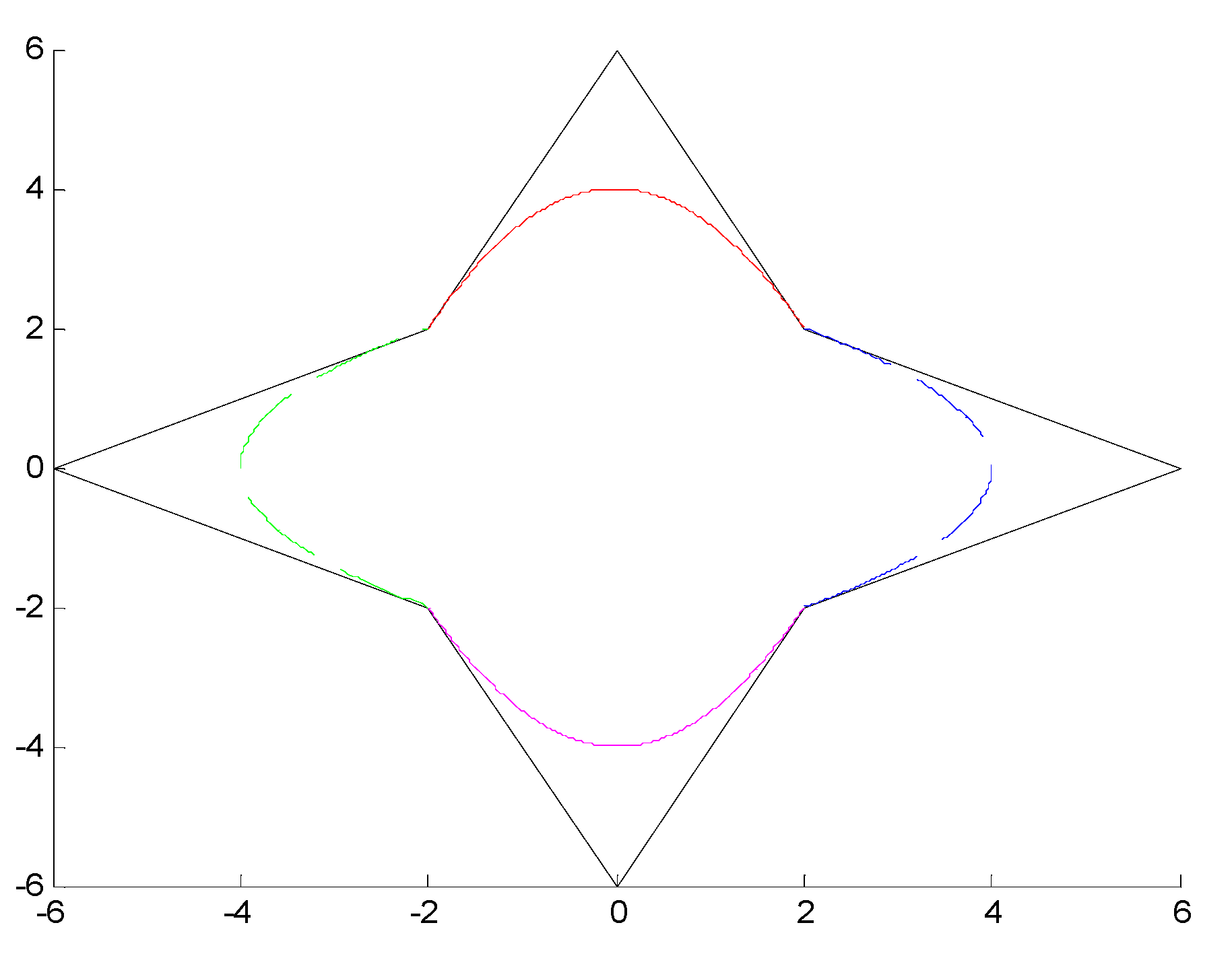
Figure 1 shows an example of G⁰ (namely C⁰) smooth continuity of four quadratic S-λ curves with the generating functions$S_1(x)=1+4x,S_2(x)=1+7x,S_3(x)=1+5x,S_4(x)=1+9x$. The corresponding sets of control points are {(−2,2), (0,6), (2,2)}, {(2,2), (6,0), (2,−2)}, {(2,−2), (0,−6), (−2,−2) } {(−2,−2), (−6,0), (−2,2)}, respectively.

Example 2.

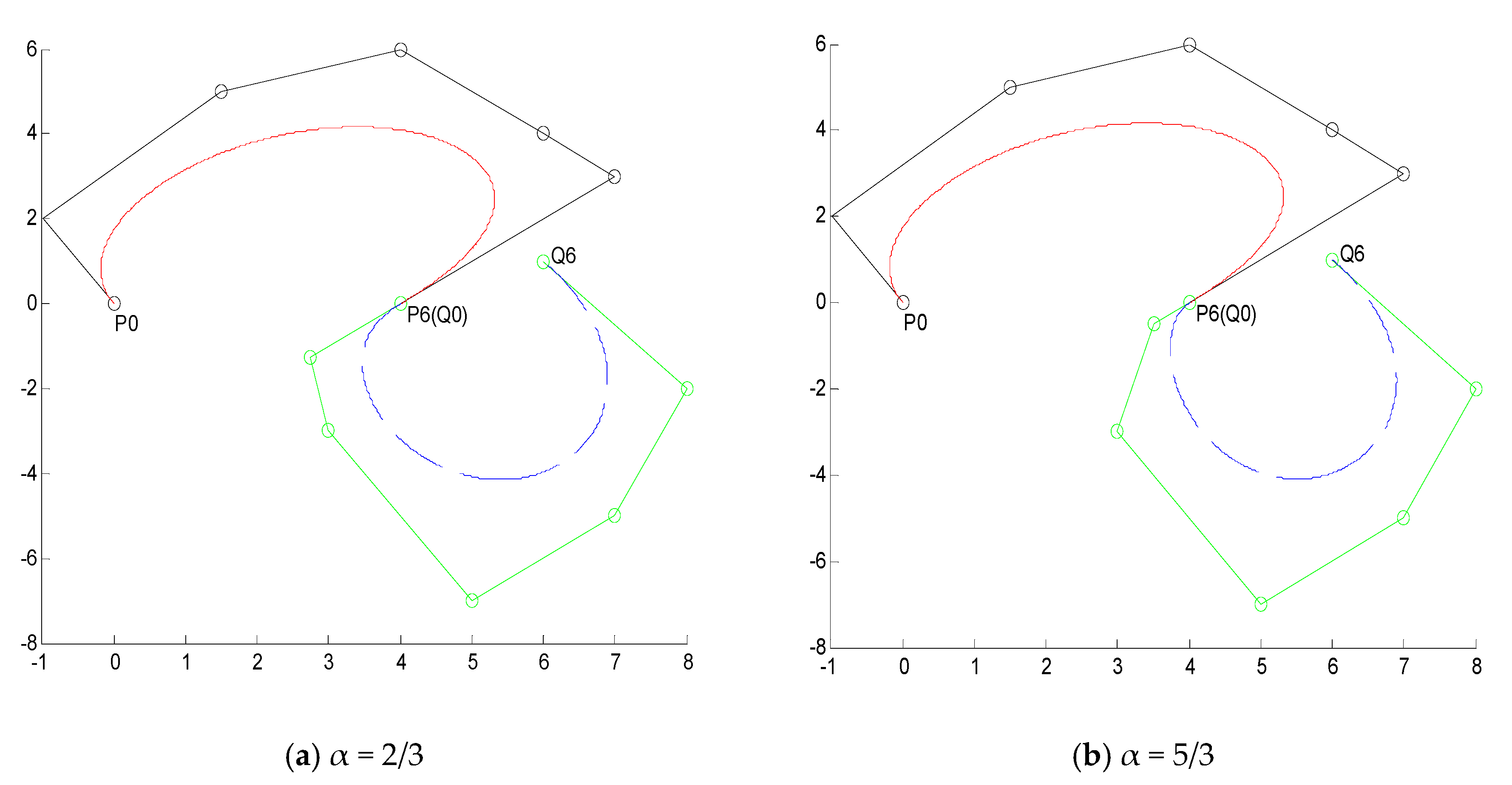
Figure 2 displays a modeling example to demonstrate the G¹ smooth continuity between two S-λ curves of degree 6 and modifies the shape of composite surface by changing the ratio of tangent vector without changing the continuous conditions. In Figure 2, the red curves represent the original curves$P(x)$, the blue curves are the constructed curves$Q(x)$which satisfy the G¹ smooth continuity conditions, that is (32). The generating functions of$P(x)$and$Q(x)$are$S_1(x)=1+4x+5x^2+6x^3$and$S_2(x)=1+3x+6x^2+4x^3$, respectively. In Figure 2a, the set of control points of S-λ curve$P(x)$and$Q(x)$are P = {(0,0), (−1,2), (1.5,5), (4,6), (6,4), (7,3), (4,0)}, Q = {(4,0), (33/12,−5/4), (3,−3), (5,−7), (7,−5), (8,−2), (6,1)}. In addition, the ratio of tangent vector of two S-λ curves is α = 2/3. In Figure 2b, we take α = 5/3, the control points of S-λ curve $P(t)$ remain unchanged, the set of control points of S-λ curve $Q(x)$ is changed to Q = {(4,0), (7/2,−1/2), (3,−3), (5,−7), (7,−5), (8,−2), (6,1)}.

Example 3.

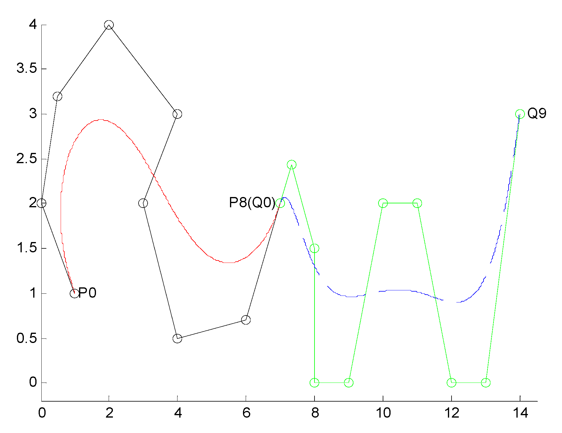
Figure 3 shows an example to illustrate the C¹ smooth continuity between a S-λ curve of degree 8 and a S-λ curve of degree 9. The generating functions of$P(x)$and$Q(x)$are$S_1(x)=1+4x+5x^2+3x^3+2x^4$and$S_2(x)=1+3x+6x^2+4x^3$. The sets of control points of S-λ curve$P(x)$and$Q(x)$are P = {(1,1), (0,2), (0.5,3.2), (2,4), (4,3), (3,2), (4,0.5), (6,0.7), (7,2)}, Q = {(7,2), (22/3,73/30), (8,1.5), (8,0), (9,0), (10,2), (11,2), (12,0), (13,0), (14,3)}, respectively.

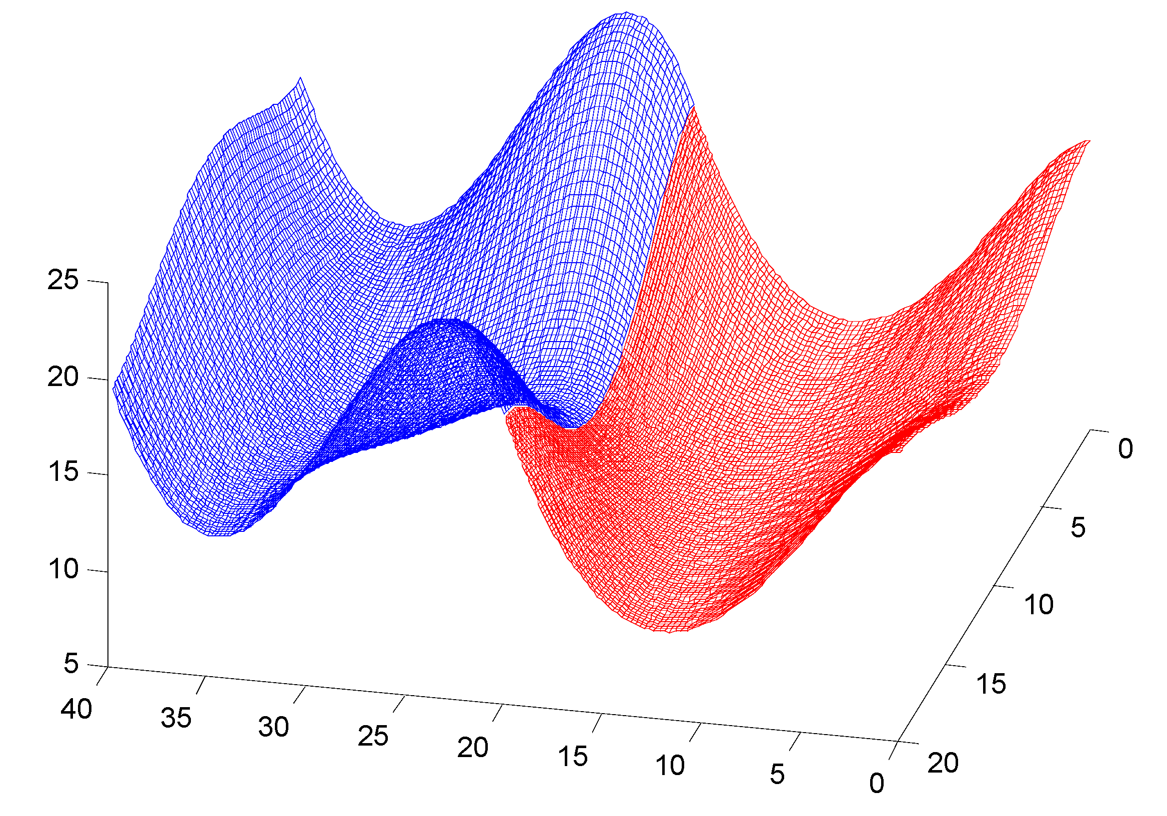
Example 4.

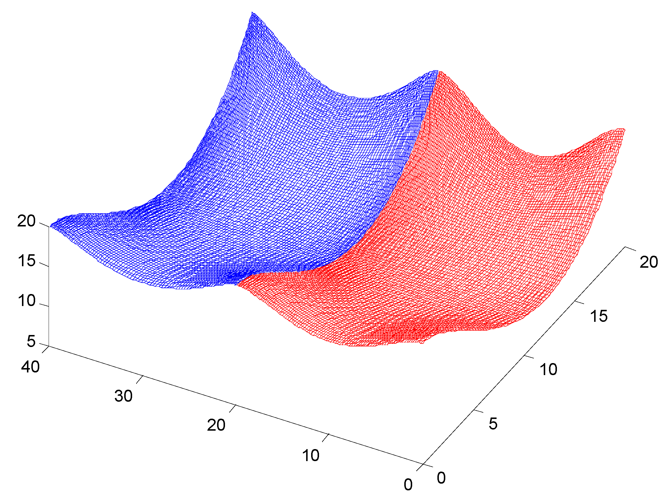
Figure 4 displays a modeling example to illustrate the G¹ smooth continuity in the u direction between two S-λ surfaces. In Figure 4, the red mesh surface represents the original surface$C_1(s,t)$, the blue mesh surface is the constructed surface$C_2(s,t)$which satisfies the G¹ smooth continuity conditions in the u direction, that is Equation (57). In addition, the basis functions of$C_1(s,t)$and$C_2(s,t)$are$P_{<m,n>,<i,j>}(s,t)=P{F}_{m,i}(s)P{G}_{n,j}(t)$and$P_{<m,k>,<i,j>}(s,t)=P{F}_{m,i}(s)P{Q}_{k,j}(t)$, where

$$P{F}_{m,i}(s)=\frac{A_i^{(m)}{[{\lambda }_1(s)]}^i}{{\left[F\left({\lambda }_1(s)\right)\right]}^m} ,P{G}_{n,j}(t)=\frac{B_j^{(n)}{[{\lambda }_2(t)]}^j}{{\left[G\left({\lambda }_2(t)\right)\right]}^n},P{Q}_{k,j}=\frac{C_j^{(k)}{[{\lambda }_2(t)]}^j}{{\left[Q\left({\lambda }_2(t)\right)\right]}^k},$$

and

$$F(x)=1+2 x+3x^2,G(x)= 1+2x+2x^2, Q(x)=1+x+2x^2,{\lambda }_1(s)=\frac{s}{1-s},{\lambda }_2(t)=\frac{t}{1-t},s\times t\in [0,1)\times [0,1)$$

The control points of S-λ surfaces$C_1(s,t)$and$C_2(s,t)$are {(0,0,20), (0,5,20), (0,10,10), (0,15,20), (0,20,20); (5,0,20), (5,5,20), (5,10,10), (5,15,20), (5,20,20); (10,0,0), (10,5,0), (10,10,10), (10,15,0), (10,20,0); (15,0,5), (15,5,5), (15,10,15),(15,15,5), (15,20,5); (20,0,20), (20,5,20),(20,10,0), (20,15,20), (20,20,20)} and {(0,20,20), (0,25,20), (0,30,10), (0,35,20), (0,40,20); (5,20,20), (5,25,20), (5,30,10), (5,35,20), (5,40,20); (10,20,0), (10,25,0), (10,30,10), (10,35,0), (10,40,0); (15,20,5), (15,25,5), (15,30,15), (15,35,5), (15,40,5); (20,20,20), (20,25,20), (20,30,0), (20,35, 20), (20,40,20)}, respectively.

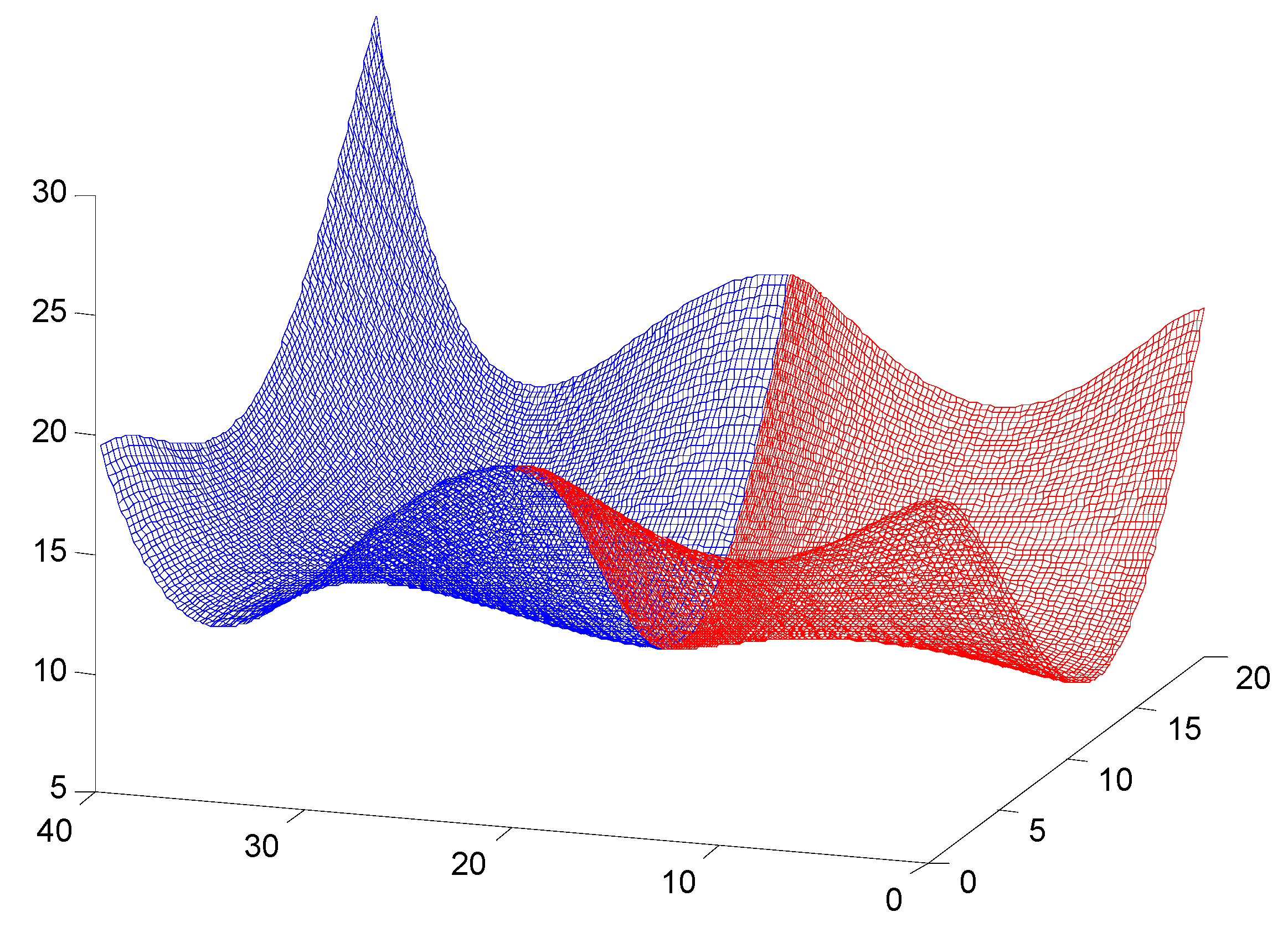
Example 5.

Figure 5 shows a modeling example to demonstrate the G¹ smooth continuity in the v direction between two S-λ surfaces. In Figure 5, the red mesh surface represents the original surface$C_1(s,t)$, the blue mesh surface is the constructed surface$C_2(s,t)$which satisfies the G¹ smooth continuity conditions in the v direction, that is Equation (58). In addition, the basis functions of$C_1(s,t)$and$C_2(s,t)$are$P_{<m,n>,<i,j>}(s,t)=P{F}_{m,i}(s)P{G}_{n,j}(t)$and$P_{<k,n>,<i,j>}(s,t)=P{Q}_{k,i}(s)P{G}_{n,j}(t)$, where

$$P{F}_{m,i}(s)=\frac{A_i^{(m)}{[{\lambda }_1(s)]}^i}{{\left[F\left({\lambda }_1(s)\right)\right]}^m},P{G}_{n,j}(t)=\frac{B_j^{(n)}{[{\lambda }_2(t)]}^j}{{\left[G\left({\lambda }_2(t)\right)\right]}^n} , P{Q}_{k,i}(s)=\frac{C_i^{(k)}{[{\lambda }_1(s)]}^i}{{\left[Q\left({\lambda }_1(s)\right)\right]}^k},$$

and

$$F(x)=1+2 x+4x^2,G(x)= 1+3x+2x^2,Q(x)=1+2x+x^2,{\lambda }_1(s)=\frac{s}{1-s},{\lambda }_2(t)=\frac{t}{1-t},s\times t\in [0,1)\times [0,1)$$

The control points of S-λ surfaces$C_1(s,t)$and$C_2(s,t)$are {(0,0,20), (0,5,20), (0,10,10), (0,15,20), (0, 20,20); (5,0,20), (5,5,20), (5,10,10), (5,15,20), (5,20,20); (10,0,0), (10,5,0), (10,10,10), (10,15,0), (10, 20,0); (15,0,5), (15,5,5), (15,10,15), (15,15,5), (15,20,5); (20,0,20), (20,5,20), (20,10,0), (20,15,20), (20,20,20)} and {(20,0,20), (20,5,20), (20,10,0), (20,15,20), (20,20,20); (25,0,35), (25,5,35), (25,10,−15), (25,15,35), (25,20,35); (30,0,10), (30,5,10), (30,10,0), (30,15,10), (30,20,10); (35,0,5), (35,5,5), (35,10,15), (35,15,5), (35,20,5); (40,0,20), (40,5,20), (40,10,30), (40,15, 20), (40,20,20)}.

Example 6.

Figure 6 shows an example to display the G¹ smooth continuity in the u and v direction between two S-λ surfaces. In Figure 6, the red mesh surface represents the original surface$C_1(s,t)$, the blue mesh surface is the constructed surface$C_2(s,t)$which satisfies the G¹ continuity conditions in the u and v direction, that is (59). Furthermore, the basis functions of$C_1(s,t)$and$C_2(s,t)$are$P_{<m,n>,<i,j>}(s,t)=P{F}_{m,i}(s)P{G}_{n,j}(t)$and$P_{<k,m>,<i,j>}(s,t)=P{Q}_{k,i}(s)P{F}_{m,j}(t)$, where

$$P{F}_{m,i}(s)=\frac{A_i^{(m)}{[{\lambda }_1(s)]}^i}{{\left[F\left({\lambda }_1(s)\right)\right]}^m}, P{G}_{n,j}(t)=\frac{B_j^{(n)}{[{\lambda }_2(t)]}^j}{{\left[G\left({\lambda }_2(t)\right)\right]}^n} ,P{Q}_{k,i}(s)=\frac{C_i^{(k)}{[{\lambda }_2(s)]}^i}{{\left[Q\left({\lambda }_2(s)\right)\right]}^k},P{F}_{m,j}(t)=\frac{A_j^{(m)}{[{\lambda }_1(t)]}^j}{{\left[F\left({\lambda }_1(t)\right)\right]}^m},$$

and

$$F(x)=1+4 x+3x^2,G(x)= 1+2x+5x^2,Q(x)=1+3x+2x^2,{\lambda }_1(s)=\frac{s}{1-s},{\lambda }_2(t)=\frac{t}{1-t},s\times t\in [0,1)\times [0,1)$$

The control points of S-λ surfaces$C_1(s,t)$and$C_2(s,t)$are {(0,0,20), (0,5,20), (0,10,10), (0,15,20), (0,20,20); (5,0,20), (5,5,20), (5,10,10), (5,15,20), (5,20,20); (10,0,0), (10,5,0), (10,10,10), (10,15,0), (10,20,0); (15,0,5), (15,5,5), (15,10,15), (15,15,5), (15,20,5); (20,0,20), (20,5,20), (20,10,0), (20,15,20), (20,20,20)} and {(0,20,20), (5,20,20), (10,20,0), (15,20,5), (20,20,20); (0,25,20), (5,25,20), (10,25,0), (15,25,5), (20,25, 20); (0,30,15), (5,30,15), (10,30,10), (15,30,5), (20,30,15); (0,35,5), (5,35,5), (10,35,15), (15,35,5), (20,35,5); (0,40,20), (5,40,20), (10,40,10), (15,40,20), (20,40,30)}.

5. Conclusions

In this paper, we introduced the S-λ curves and surfaces and derived the geometric conditions for G¹ smooth continuity between two adjacent S-λ curves and surfaces, respectively. In addition—in terms of the proposed continuity conditions—some modeling examples are provided to verify the effectiveness of the method. In summary, the research in this paper not only provides a unified method for dealing with common geometric models (such as the Bézier model, the B-spline model and the Poisson model), but also provides a practical technology with distinctive characteristics for the CAGD system. The advantages of the S-λ model can be summarized as follows:

(a)

The G¹ smooth continuity conditions for S-λ curves and surfaces proposed in this paper extend the conclusions of S-λ model constructed by Fan and Zeng [6,7];

(b)

For any composite S-λ curves and surfaces which satisfy G¹ or C¹ geometric continuity, its local and global shape can be adjusted flexibly by modifying the shape parameters without changing the control points;

(c)

S-λ model can be transformed into different geometric models when the generating functions and transformation factors of the S-λ basis functions are different, so the research of this paper plays an important role in the complex modeling design of other common geometric models as well.

It is noteworthy that the G¹ geometric continuity conditions of S-λ curves and surfaces are studied for the first time in this paper. We will focus on studying the G² geometric continuity conditions of S-λ model in future work. In addition, some interesting directions for future research would be to implement the performance and esthetics comparison of S-λ methods with other methods.

References

- Johnson, N.L.; Kemp, A.W.; Kotz, S. Univariate Discrete Distributions; John Wiley & Sons, Inc.: Hoboken, NJ, USA, 2005. [Google Scholar]
- Poston, W.L.; Johnson, N.L.; Kotz, S. Discrete Multivariate Distributions; Wiley: Hoboken, NJ, USA, 1998; Volume 40, p. 160. [Google Scholar]
- Goldman, R.N. Urn models and B-splines. Constr. Approx. 1988, 4, 265–288. [Google Scholar] [CrossRef]
- Goldman, R.N. The rational Bernstein bases and the multirational blossoms. Comput. Aided Geom. Des. 1999, 16, 701–738. [Google Scholar] [CrossRef]
- Morin, G.; Goldman, R.N. A subdivision scheme for Poisson curves and surfaces. Comput. Aided Geom. Des. 2000, 17, 813–833. [Google Scholar] [CrossRef]
- Fan, F.L.; Zeng, X.M. S-λ basis functions and S-λ curves. Comput. Aided Des. 2012, 44, 1049–1055. [Google Scholar] [CrossRef]
- Zhou, G.R.; Zeng, X.M.; Fan, F.L. Bivariate S-λ bases and S-λ surface patches. Comput. Aided Geom. Des. 2014, 31, 674–688. [Google Scholar] [CrossRef]
- Lu, J.; Qin, X.Q. Degree Reduction of S-λ Curves Using a Genetic Simulated Annealing Algorithm. Symmetry 2018, 11, 15. [Google Scholar] [CrossRef] [Green Version]
- Chen, S.N.; Zhao, C.; Zeng, X.M. A New Shape Adjustment Method of S-λ Curve. Comput. Aided Draft. Des. Manuf. 2014, 24, 39–43. [Google Scholar]
- Zeng, X.M.; Lin, L. On limiting properties of Bernstein–Trotter type operator. J. Math. Study 1994, 27, 200–203. [Google Scholar]
- Zhao, J.H. Quantify behaviors of approximation degree to unbounded functions by generalized Feller operators derived S–λ. Acta Math. Sci. 1997, 17, 466–472. [Google Scholar]
- Shi, F.Z. Computer Aided Geometric Design and NURBS; China Higher Education Press: Beijing, China, 2001. [Google Scholar]
- Liu, D.; Hoschek, J. GC1 continuity conditions between adjacent rectangular and triangular Bezier surface patches. Comput. Aided Des. 1989, 21, 194–200. [Google Scholar] [CrossRef]
- Degen, W.L.F. Explicit continuity conditions for adjacent Bézier surface patches. Comput. Aided Geom. Des. 1990, 7, 181–189. [Google Scholar] [CrossRef]
- Liu, D.Y. GC1 continuity conditions between two adjacent rational Bézier surface patches. Comput. Aided Geom. Des. 1990, 7, 151–163. [Google Scholar] [CrossRef]
- Chui, C.K.; Lai, M.J.; Lian, J.A. Algorithms for G1 connection of multiple parametric bicubic NURBS surfaces. Numer. Algorithms 2000, 23, 285–313. [Google Scholar] [CrossRef]
- Konno, K.; Tokuyama, Y.; Chiyokura, H. A G1 connection around complicated curve meshes using C1 NURBS Boundary Gregory Patches. Comput. Aided Des. 2001, 33, 293–306. [Google Scholar] [CrossRef]
- Yu, P.Q.; Shi, X.Q. G1 continuous conditions for bicubic NURBS surfaces. J. Dalian Univ. Technol. 2004, 44, 330–333. [Google Scholar]
- Wu, L.S.; Gao, X.Q.; Xiong, H. Improved curve surface seamless splicing based on NURBS. Opt. Precis. Eng. 2013, 21, 431–436. [Google Scholar]
- Hu, G.; Zhang, G.; Wu, J.L.; Qin, X.Q. A novel extension of the Bézier model and its applications to surface modeling. Adv. Eng. Softw. 2018, 125, 27–54. [Google Scholar] [CrossRef]
- Hu, G.; Bo, C.; Wu, J.; Wei, G.; Hou, F. Modeling of free-form complex curves using SG-Bézier curves with constraints of geometric continuities. Symmetry 2018, 10, 545. [Google Scholar] [CrossRef] [Green Version]
- Hu, G.; Bo, C.C.; Wei, G.; Qin, X.Q. Shape-adjustable generalized Bézier Surfaces: Construction and its geometric continuity conditions. Appl. Math. Comput. 2020, 378, 125215. [Google Scholar]
- Hu, G.; Bo, C.C.; Qin, X.Q. Continuity conditions for Q-Bézier curves of degree n. J. Inequalities Appl. 2017, 115, 1–14. [Google Scholar] [CrossRef] [Green Version]
- Hu, G.; Bo, C.; Qin, X. Continuity conditions for tensor product Q-Bézier surfaces of degree (m, n). Comp. Appl. Math. 2018, 37, 4237–4258. [Google Scholar] [CrossRef]
- Qian, J.; Tang, Y. The application of H-Bézier-like curves in engineering. Numer. Methods Comput. Appl. 2007, 28, 167–178. [Google Scholar]
- Usman, M.; Abbas, M.; Miura, K.T. Some engineering applications of new trigonometric cubic Bezier-like curves to free-form complex curve modeling. J. Adv. Mech. Des. Syst. 2020, 14, jamdsm0048. [Google Scholar] [CrossRef] [Green Version]
- Bibi, S.; Abbas, M.; Miura, K.T.; Misro, M.Y. Geometric Modeling of Novel Generalized Hybrid Trigonometric Bézier-Like Curve with Shape Parameters and Its Applications. Mathematics 2020, 8, 967. [Google Scholar] [CrossRef]
- Li, F.; Hu, G.; Abbas, M.; Miura, K.T. The generalized H-Bézier model: Geometric continuity conditions and applications to curve and surface modeling. Mathematics 2020, 8, 924. [Google Scholar] [CrossRef]
- Hu, G.; Wu, J.L. Generalized quartic H-Bézier curves: Construction and application to developable surfaces. Adv. Eng. Softw. 2019, 138, 102723. [Google Scholar] [CrossRef]
- Hu, G.; Cao, H.X.; Zhang, S.X.; Wei, G. Developable Bézier-like surfaces with multiple shape parameters and its continuity conditions. Appl. Math. Model. 2017, 45, 728–747. [Google Scholar] [CrossRef]
Figure 1.
G0(also C0) smooth continuity of quadratic S-λ curves.
Figure 2.
G1 smooth continuity of two sextic S-λ curves.
Figure 3.
C1 smooth continuity of S-λ curves.
Figure 4.
G1 smooth continuity of two S-λ surfaces in the u direction.
Figure 5.
G1 smooth continuity of two S-λ surfaces in the v direction.
Figure 6.
G1 smooth continuity of two S-λ surfaces in the u and v direction.
© 2020 by the authors. Licensee MDPI, Basel, Switzerland. This article is an open access article distributed under the terms and conditions of the Creative Commons Attribution (CC BY) license (http://creativecommons.org/licenses/by/4.0/).
Share and Cite
MDPI and ACS Style
Hu, G.; Li, H.; Abbas, M.; Miura, K.T.; Wei, G. Explicit Continuity Conditions for G1 Connection of S-λ Curves and Surfaces. Mathematics 2020, 8, 1359. https://0-doi-org.brum.beds.ac.uk/10.3390/math8081359
AMA Style
Hu G, Li H, Abbas M, Miura KT, Wei G. Explicit Continuity Conditions for G1 Connection of S-λ Curves and Surfaces. Mathematics. 2020; 8(8):1359. https://0-doi-org.brum.beds.ac.uk/10.3390/math8081359
Chicago/Turabian StyleHu, Gang, Huinan Li, Muhammad Abbas, Kenjiro T. Miura, and Guoling Wei. 2020. "Explicit Continuity Conditions for G1 Connection of S-λ Curves and Surfaces" Mathematics 8, no. 8: 1359. https://0-doi-org.brum.beds.ac.uk/10.3390/math8081359
Note that from the first issue of 2016, this journal uses article numbers instead of page numbers. See further details here.