Improved Performance of M-Class PMUs Based on a Magnitude Compensation Model for Wide Frequency Deviations

Abstract

Phasor measurement units (PMUs) are important elements in power systems to monitor and know the real network condition. In order to regulate the performance of PMUs, the IEEE Std. C37.118.1 stablishes two classes—P and M, where the phasor estimation is carried out using a quadrature oscillator and a low-pass (LP) filter for modulation and demodulation, respectively. The LP filter plays the most important role since it determines the accuracy, response time and rejection capability of both harmonics and aliased signals. In this regard and by considering that the M-class filters are used for more accurate measurements, the IEEE Std. presents different M-class filters for different reporting rates (when a result is given). However, they can degrade their performance under frequency deviations if the LP frequency response is not properly considered. In this work, a unified model for magnitude compensation under frequency deviations for all the M-class filters is proposed, providing the necessary values of compensation to improve their performance. The model considers the magnitude response of the M-class filters for different reporting rates, a normalized frequency range based on frequency dilation and a fitted two-variable function. The effectiveness of the proposal is verified using both static and dynamic conditions for frequency deviations. Besides that, a real-time simulator to generate test signals is also used to validate the proposed methodology.

1. Introduction

Over the past few years, phasor measurement units (PMUs) have become key elements in many applications of power systems, for example, monitoring, protection, control, renewable energy integration, fault location and instrument transformers calibration [1,2,3,4,5]. PMUs are devices that provide measurements of magnitude, phase, frequency and rate of change of frequency (ROCOF) for voltage and current signals in a synchronous way [1]. In order to regulate the performance of PMUs, the IEEE Std. C37.118.1 sets several tests and requirements under both static and dynamic conditions for evaluating the measurement quality [6,7]. Besides that, this Std. presents a reference signal processing algorithm used to estimate the phasor information, which in general, consists of a quadrature oscillator for modulation and a low-pass (LP) filter for demodulation [5,6]. The principal difference between P-class and M-class relies on the LP filter used for demodulation as it determines the accuracy, response time and rejection capability of both harmonics and aliased signals, among many other parameters [6]. In particular, M-class filters are intended for applications that could degrade their performance under aliased signals [8]; hence, their formulation is more complex since a higher accuracy is demanded. Despite being powerful and robust devices, PMUs can degrade their accuracy when they are subjected to waveforms of voltage and current that contain—modulations, sudden and abrupt changes of magnitude and/or phase angle and large frequency deviations [8]. These unwanted waveforms are associated with the dynamic load behavior, embedded generation and renewable sources of energy, among others [9,10,11,12]. One of the reasons why frequency deviations occur in autonomous networks is due to one-site generators [13]. Also, the use of renewable energy sources such as wind turbines implies a variable power generation, sometimes resulting in frequency deviations, low-frequency values are also observed during the start-up and shut-down of generators in power systems [14]. These non-nominal frequency values (ranging from a few Hz up to 100% of the nominal value in some cases) cause equipment malfunction and, if the frequency, magnitude and phase (information provided by a PMU) are not correctly measured, degradation of the performance of protections, controllers and state estimators, among other negative effects, occurs [15,16,17]. Moreover, wide frequency deviations can be also observed during a possible collapse of the power system, where the generator is shut down and the frequency goes down to zero; in this case, a PMU that can deal with wide frequency deviations will allow get important information about the transient stability of the system [18]. Other possible use is in the monitoring and control of AC-AC or AC-DC-AC converters, which are used to transfer power between two systems with different frequency such as the wind turbines with variable speed interconnected with the power grid [19].

In this regard, the analysis of PMUs under signal frequency deviations has received special attention since they are directly related to the performance of the LP filters used in PMUs [20]. In other words, the output signal suffers magnitude and phase changes due to the LP filter frequency response, requiring a compensation stage if reliable and accurate results are needed, mainly considering that estimation errors may lead to undesirable results for PMUs applications. From this point of view, the development of compensation strategies to minimize the adverse impacts of frequency deviations in the accuracy of results in PMUs is still a hot research topic for power systems, especially if large frequency deviations associated to changes in the electric power generation, failures in the power system, integration of renewable energies [21] and microgrids [22] are taken into consideration.

Previous methodologies that fulfill the requirements stated in the IEEE Std. C37.118.1 use techniques such as Taylor series [23], empirical wavelet transform [24], interpolated discrete Fourier Transform (DFT) and Taylor-Fourier transform [25], Taylor weighted least square [26], frequency tracking and fixed-filters [27]; however, they only cover a limited frequency range stablished by the IEEE Std. C37.118.1. On the other hand, some works that improve the performance of PMUs have been presented in the literature, where new phasor estimation algorithms, new adaptive filtering-based methodologies and several compensation strategies have been proposed [1,6,8,21,22,23,24]. For instance, some remarks about the performance of PMUs under dynamic conditions for electric signals are presented in References [28,29,30]. Regarding the compensation strategies, the phase is compensated using input delays, due to the linear phase characteristics of the filters. Also, the magnitude compensation for signal frequency deviations is presented in the Std. of PMUs [6]; however, it only presents the compensation model for the P-class filter. Note that the Std. mentions that the magnitude estimation under frequency deviations can be compensated as follows—divide the phasor magnitude by the magnitude frequency response of the P-class filter. This can be carried out in a simpler way using the evaluation of a model based on a sine function at the measured frequency, which has an argument obtained experimentally [6]; however, this compensation only works over a limited frequency range. As above-mentioned, the Std. does not present a compensation model for the M-class filter, which could compromise the accuracy under frequency deviations, even those that are close to 55 or 65 Hz [31]. The compensation methodology for the M-class PMUs is not a straightforward process since the Std. presents a set of LP filters with different specifications such as filter order and reference frequency for each reporting rate stated [6], which increases the complexity of the problem. It is worth noting that the different M-class filters are required to fulfill the Std. requirements, mainly the rejection capability of the aliased components [6]. Other schemes using adaptive approaches that consider the accuracy and performance of PMUs under wide frequency deviation ranges are presented in References [1,8]. A finite-impulse-response (FIR) bandpass filter, the extended Kalman filter and a discrete Fourier transform demodulation with a FIR-LP filter algorithm were presented by Reference [8] as adaptive schemes for PMUs. They can achieve a reliable and suitable operation under different wide frequency deviation conditions, for example a frequency range from 45 to 75 Hz is achieved for a 1 Hz/s frequency ramp. Adaptive cascade filters in compliance with the IEEE Std. C37.118.1 for P and M class filters were proposed [1]. The authors consider two variants named tick-tock and asymmetric, achieving accurate results over wide frequency ranges (±33% of the nominal frequency). Although enhanced results are obtained, the compensation of the estimated magnitude under large frequency deviations for the M-class filters as specified by the IEEE Std. C37.118.1 for each reporting rate has not been reported.

In this work, a novel methodology to obtain a general model for magnitude compensation under signal frequency deviations for the M-class filters at different reporting rates, according to the IEEE Std. C37.118.1, is proposed. It is worth mentioning that all the M-class filters have to be considered as they fulfill the requirements stated in the mentioned Std. for different reporting rates, mainly the rejection capability of aliased components. In order to design a general and unified compensation model, the proposed methodology dilates the magnitude frequency responses of the LP filters for each reporting rate and fits a three-dimensional (3D) function. This function involves the frequency deviation, the reporting rate and the magnitude frequency responses. In this regard, commercial M-class PMUs can include the proposed compensation function to provide the compensation factor required to improve the PMU performance at different reporting rates, which are defined by the end user. Moreover, as the main advantage, the proposed model offers the correct magnitude estimation using a compensation stage for wide frequency deviation ranges, outperforming the ranges stated by both the Std. and the different methodologies presented in the literature. In order to demonstrate both the effectiveness of the proposal to compensate the magnitude estimation under wide frequency deviations and its compliance with the mentioned Std., the frequency test in steady-state and the dynamic test are carried out. As the reporting rate determines the measurement bandwidth [32], different ranges and parameters have to be considered. It is worth noting that, in this research work, other compliance tests such as out of band, modulation, harmonic content and step change are not carried out since the proposal uses, as reference filters, the signal processing models provided by the Std. (M-class filters), which have already been tested; besides, these tests are not related with frequency deviations. Although tests for sinusoidal frequency variations are not considered in the Std., a study case is also presented since those oscillations can occur in real power systems [33,34,35,36]. The obtained results show that total vector error (TVE) is less than 1% for a wide frequency deviation range. Real voltage signals with off-nominal frequencies are also analyzed, which are generated and acquired using a real-time simulator.

2. Theoretical Background

2.1. IEEE Std. C37.118.1

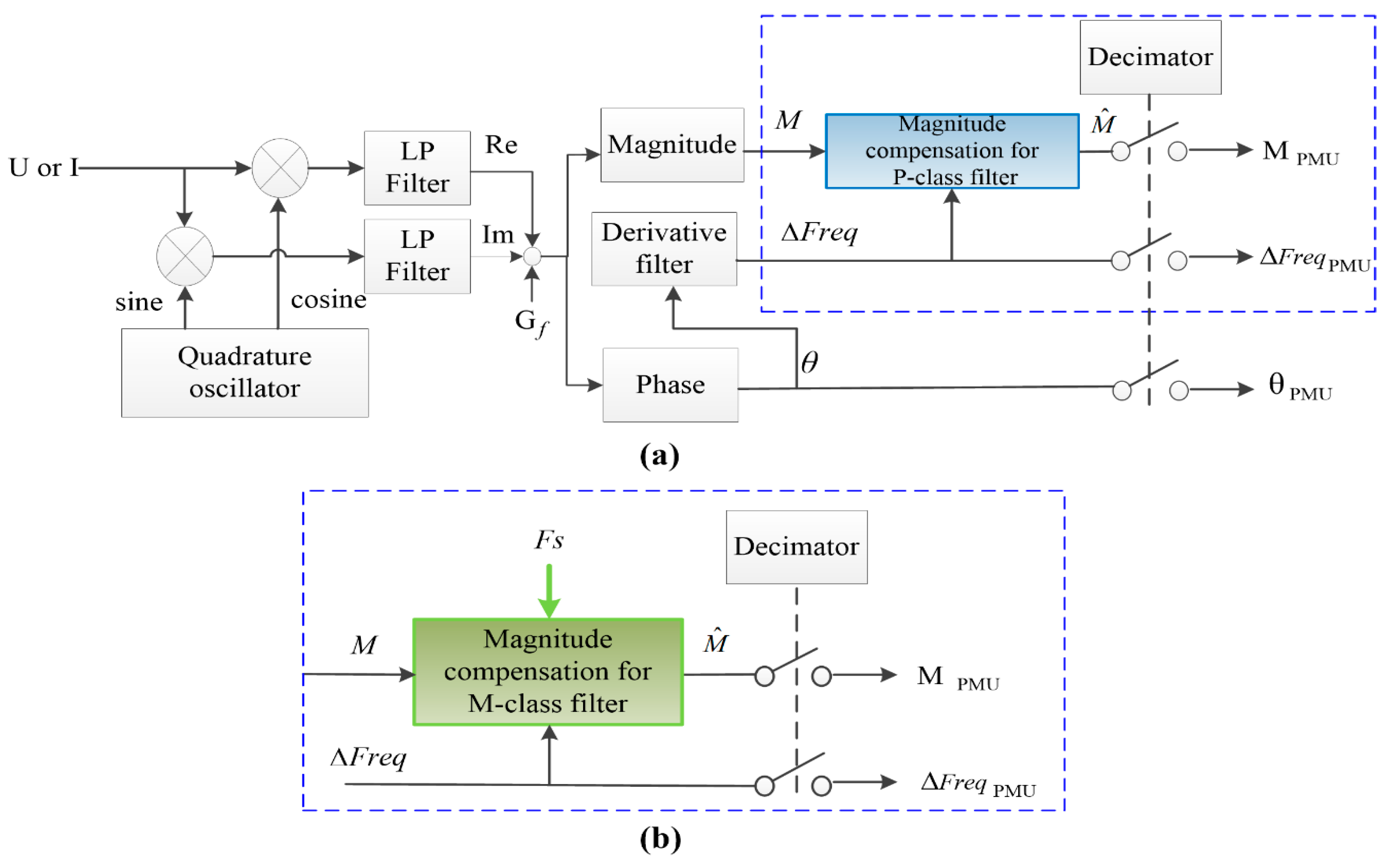
The IEEE Std. C37.118.1 sets two classes of PMUs [6], that is, P class and M class. Their selection depends basically on the desired application [37]. The Std. presents a reference algorithm for PMUs with the freedom of using any appropriate technique that can be developed for satisfying steady-state and dynamic conditions. Figure 1a shows the general structure of the signal processing algorithm for the PMU [6]. In general, the processing algorithm provided by the IEEE Std. C37.118.1 can be described as follows—firstly, the voltage or current signal, U or I, are sampled through a fixed sampling frequency. Then, the signal is modulated by a carrier signal using a complex multiplication, which is implemented using a quadrature oscillator (sine and cosine signals at nominal frequency). Next, the LP filter for each signal is used for demodulation. For obtaining a unity gain at the DC component (0 Hz), the transfer function is divided by a compensation gain, G_DC, which is obtained by adding the coefficients of the LP filters. It is worth mentioning that the Std. presents different filters for each class of PMUs—one filter for the P-class (one for all the reporting rates) and a set of filters for the M-class (one for each reporting rate). The LP filter outputs represent the real (Re) and Imaginary (Im) parts of a complex signal, Re + Im·i. Therefore, the root mean square (RMS) magnitude, M and the phase angle, θ, are obtained as follows:

$$M=\frac{1}{\sqrt{2}}\sqrt{R{e}^2+I{m}^2},\theta =ta{n}^{-1}\left(\frac{Im}{Re}\right).$$

(1)

The frequency deviation, ΔFreq, is estimated by⁵:

$$\Delta Freq\left(n\right)=\frac{\left(6\left[\theta \left(n\right)-\theta \left(n-1\right)\right]+3\left[\theta \left(n-1\right)-\theta \left(n-2\right)\right]+\left[\theta \left(n-2\right)-\theta \left(n-3\right)\right]\right)}{20\pi /F_{sampling}}$$

(2)

where θ(n − m), for m = 0, 1, 2 and 3, represents the phase angle results at the sample denoted by (n − m), n is the sample and F_sampling is the sampling frequency. It is worth noting that it can be implemented as a derivative filter.

The block of magnitude compensation, see Figure 1a, is a strategy for compensating the magnitude errors associated with frequency deviations. The magnitude compensation is carried out by:

$$\widehat{M}=\frac{M}{\left(Mode{l}_{filter-Class}\right)}$$

(3)

where M is the actual magnitude, $\widehat{M}$ is the compensated magnitude and Model_filter-Class is the compensation factor of the filter. It is worth mentioning that the Std. only provides the compensation model for P-class filters, that is, the magnitude compensation for frequency deviations, according to the IEEE Std. C37.118.1, is carried out using:

$$Mode{l}_{P-Class}=sin\left(\frac{\pi \left(f_0+K_C\Delta Freq\left(i\right)\right)}{2f_0}\right),$$

(4)

where the sine function is the model that provides, in a simple way, the magnitude frequency response of the P-class filter within a limited frequency range, ΔFreq is the measured frequency deviation, f₀ is the nominal frequency and K_C = 1.625 is a factor obtained experimentally [6]. Model_P-Class represents Model_filter-Class in (3). Also, the phase is compensated considering the group delay for the linear phase FIR filter, that is, shifting the signal (N − 1)/2 samples where N is filter order.

Finally, in Figure 1a, the magnitude (M_PMU), phase angle (θ_PMU) and frequency deviation (ΔFreq_PMU) are the decimated values from the information provided by the PMU. The decimator factor is determined by F_sampling and the reporting rate (Fs), which is given in fps, that is, the amount of results per second. In general, the PMU supports data reporting rates at sub-multiples of the nominal power-line frequency. The reporting rate has to be user selectable; for example, for 60 Hz systems, the Fs values are 10, 12, 15, 20, 30, 60 and 120 fps [6]. On the other hand, PMU results may differ from theoretical values. In this regard, the TVE is given by the Std. as a value to quantify the difference between perfect values (ideal values) and the estimation (measured values) given by the PMU under test at the same instant of time. TVE is defined by References [6,38]:

$$\begin{gathered} TVE\left(n\right)=\frac{\left|{\overrightarrow{X}}_{MEAS}-{\overrightarrow{X}}_{IDEAL}\right|}{\left|{\overrightarrow{X}}_{IDEAL}\right|} \\ TVE=\sqrt{\frac{{(X_{MEA{S}_{Re}}\left(n\right)-X_{IDEA{L}_{Re}}\left(n\right))}^2+{(X_{MEA{S}_{Im}}\left(n\right)-X_{IDEA{L}_{Im}}\left(n\right))}^2}{{(X_{IDEA{L}_{Re}}\left(n\right))}^2+{(X_{IDEA{L}_{Im}}\left(n\right))}^2}}, \end{gathered}$$

(5)

where ${\overrightarrow{X}}_{MEAS}$ and ${\overrightarrow{X}}_{IDEAL}$ are the vectors of the measured and expected (ideal) values of the phasor representation, respectively. It is worth noting that the measured values are those obtained by the in-test algorithm and the expected values are those provided by the IEEE Std. Subscripts Re and Im indicate the real and imaginary components, respectively, of the aforementioned vectors.

2.2. M-Class Filter

Unlike the P-class filter design, the M-class filter must be attenuated by at least 20 dB for any component that is above the Nyquist frequency for the corresponding reporting rate (Fs/2). The filter coefficients, W(k), are obtained using the brick-wall design methodology, which is based on a “sinc” function. Also, the filter function is multiplied by a Hamming window h(k) for ripple reduction and improvement of the attenuation factor of the stop band. Furthermore, the order of the filter is adjusted to meet frequency response requirements. The coefficients are determined by using [6]:

$$W\left(n\right)=\frac{sin\left(2\pi \frac{2F_{fr}}{F_{sampling}}n\right)}{2\pi \frac{2F_{fr}}{F_{sampling}}n}\cdot h\left(n\right),$$

(6)

where F_fr is the LP filter reference frequency, F_fr and N are presented in Table C1 in IEEE Std. C37.118.1. Finally, n goes from −N/2 to N/2 and the value of W(n) for k = 0 is replaced by 1.

The magnitude compensation for P-class PMUs is given in (4); yet, M-class PMUs require a more complex solution since the filter coefficients and N change with Fs. Besides that, the compensation function shown in (4) for P-class filters would not be enough for satisfying the requirements of the M-class filters due to the differences in their frequency responses. In this regard, a new magnitude compensation stage for the M-class filter that considers the reporting rate has to be proposed, see Figure 1b. For M-class filter, the green block is proposed to replace the blue block denoted by the dotted blue rectangle in Figure 1a. There, it can be observed that the new proposal considers two variables—ΔFreq and Fs. Therefore, it can compensate the magnitude under frequency deviations using different Fs.

In order to be compliant with the IEEE Std. C37.118.1, a set of tests in steady-state and dynamic conditions need to be carried out. In particular, the frequency test in steady-state and the linear frequency ramp as a dynamic test are only considered since they involve the conditions and values of frequency in voltage or current signals that may require magnitude compensation, mainly under wide frequency deviations. For these tests, the mathematical models presented in Reference [6] are used, where their limits and specifications are described in the next section. Also, although tests for sinusoidal frequency variations are not considered in the Std., this study case is also presented.

2.3. Steady-State and Dynamic Tests

The compliance tests have to be carried out in nominal reference conditions, except the parameters being changed in the test [6]. The mathematical models and parameters that have to be used for each test are presented in Reference [6]. As summary,

Table 1. Compliance tests for M-class PMUs.

	Steady-State Test	Dynamic Test
Description	Steady state signals with different ΔFreq	Linear frequency ramp	Sinusoidal frequency variations
Range	±2.0 Hz for Fs < 10; ±Fs/5 for 10 ≤ Fs ≤ 25; ±5 Hz for Fs ≥ 25	Lesser of ±(Fs/5) or ±5 Hz	No defined
Limit errors	TVE = 1%	TVE = 1%	No defined

shows the test description, the ranges of variation and the limits set by the Std. regarding the frequency tests. It is worth mentioning that a TVE of 1% corresponds to a maximum magnitude error of 1%, whenever the error in phase angle is zero.

On the other hand, sinusoidal frequency variations are common electrical conditions in power systems [33,34,35,36]. By considering that the proposal aims to compensate magnitude under wide frequency deviations, the aforementioned condition is also analyzed in this work although the Std. does not consider it and therefore does not define the range and limit errors. The goal is to increase the applicability of the proposal; for this test, the frequency of the signal varies sinusoidally as a function of time. In this work, the following equation is used for describing this condition.

$$X_a=X_{m}cos[2\pi f_{0}t-A_{f}cos(2\pi f_{f}t)/f_f+A_f/f_f],$$

(7)

where X_m is the amplitude of the input signal and, A_f and f_f are the amplitude and the frequency of the sinusoidal variation of the frequency, respectively. In other words, the resulting frequency varies as $f=A_f\sin (2\pi f_{f}t)+f_0$.

2.4. Applications Related to Wide Frequency Deviations

As mentioned in previous sections the electrical systems suffer different types of distortions such as modulations, sudden and abrupt changes of magnitude and/or phase angle and large frequency deviations. Specifically, frequency deviations are generated due to the connection and disconnection of heavy loads in the distribution system or short circuit faults, which in turn generates changes in the speed of the generators. In consequence, this generates serious consequences mainly in industries where there is cogeneration coupled to the grid, where the generator itself will follow the variations imposed by the electrical system, which usually are more powerful [39]. Some applications that require reliable measurements against wide frequency deviations are—in the use of renewable energy sources, during the start-up and shut-down of generators in power systems, during a possible collapse of the power system, protection and control, among other. In addition, some others applications can be highlighted such as the deployments of variable renewable energy sources, for instance photovoltaic (PV) systems, the power intermittency of PV systems causes major problems such as voltage fluctuations and frequency deviations in an electric power grid, that result in poor power quality for consumers [40]. On the other hand, the wide frequency deviation could occur due to either erroneous measurements or transient phenomena due to the interconnector trip to detect islanding system reclosure [41,42]. Another scheme where the present proposal can be used is for wide-area monitoring and control applications with variations up to 40 to 80 Hz as the one proposed in References [43,44]. Also, the wide frequency deviations occur with the high penetration of renewable energy resources in microgrids and compromise their stable operation, that is when battery energy storages are used to regulate frequency fluctuations, the battery should be charged and discharged constantly to compensate power imbalances [45]; a similar application is in wind energy storage systems [46,47]. These types of applications require accurate phasor and frequency information from multiple synchronized devices to provide a valid measurement of the dynamic behavior of the systems.

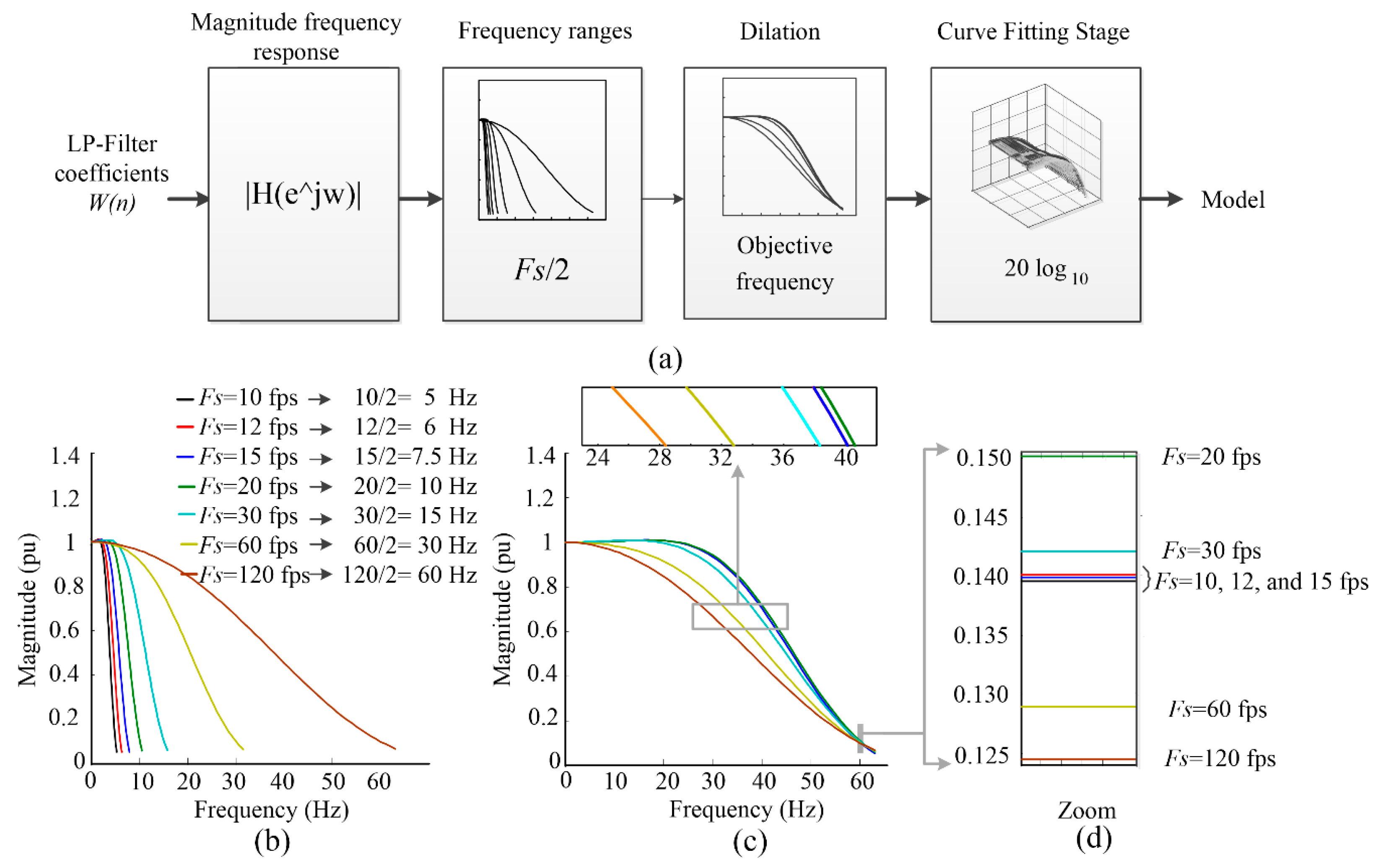
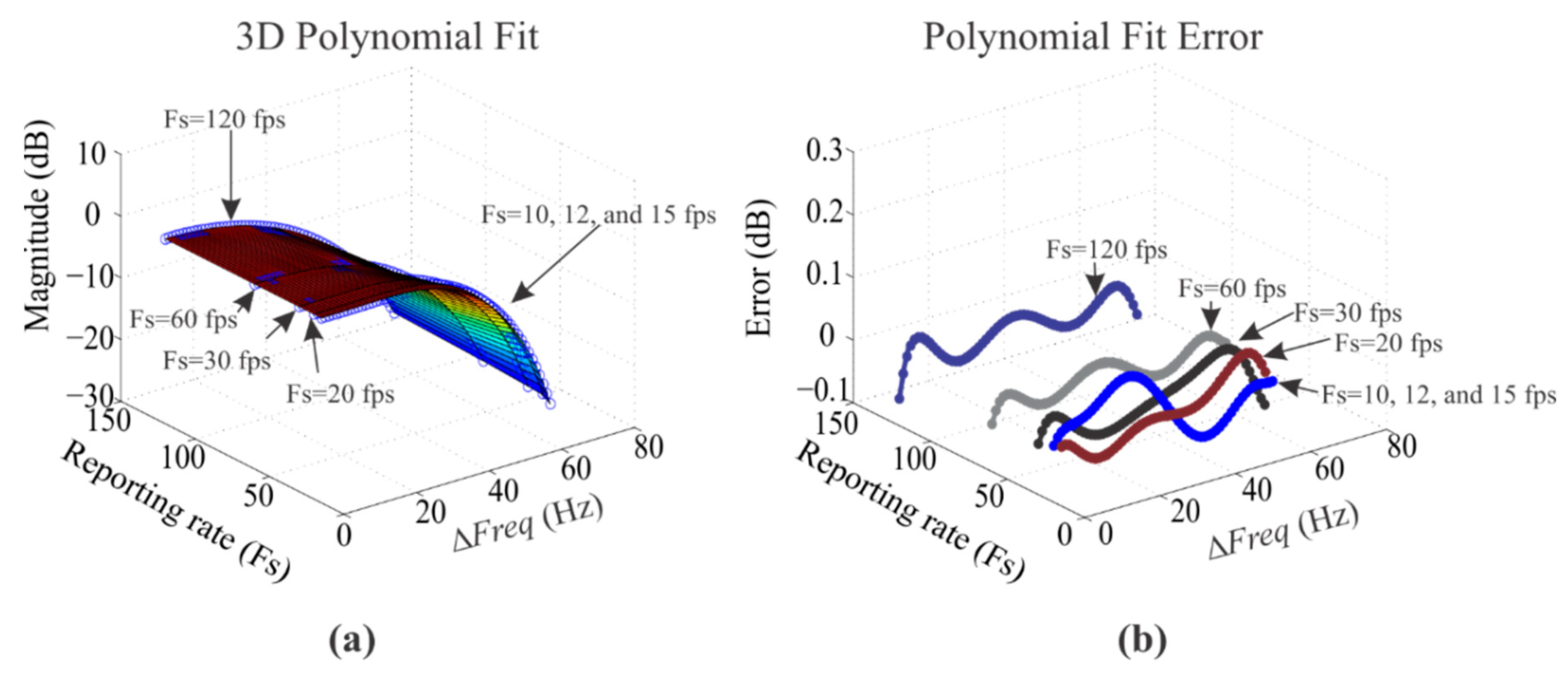
3. Proposed Methodology to Obtain the Compensation Model

As mentioned above, the proposal is a modification of the algorithm presented in the IEEE Std., which uses different filters for the estimation of magnitude and phase. These low pass filters depend on the reporting rate and are not ideal filters; therefore, the estimated magnitude is affected by the frequency of the signal. From this point of view, the proposal adds a compensation stage to the M-class PMUs for the magnitude estimation in order to be able of operating with the accuracy requirements stated in the IEEE Std. C37.118.1 but under a wider frequency range. In this regard, a methodology to obtain a general and complete compensation model by considering the seven LP filters presented in Table C1 of IEEE Std. C37.118.1 is proposed (see Figure 2). It is important to consider all the filters for different Fs, as they fulfill the requirements stated in the Std.

In general, the proposed methodology consists of four stages depicted in Figure 2a. Using the LP filter coefficients obtained by (6) and the parameters of Table 1, the first stage of the methodology determines the magnitude frequency response in the allowable frequency range (from 0 Hz to Fs/2) for each M-class filter. In other words, it determines the magnitude of each LP filter transfer function evaluated by z = e^jω, where ω = 2πf.

The next stage selects a frequency deviation range for each magnitude frequency response of the filters. In this paper, Fs/2 is selected for satisfying the Nyquist theorem requirements and achieving an attenuation of no-less than 20 dB in the first side lobe of each LP filter, where the relevant information is located (Figure 2b, pu means per unit). Next, a dilation of each curve obtained in the previous stage is performed by scaling them to a common point called objective frequency (see Figure 2c). This point represents the maximum frequency value in the allowable range, which is given by the curve for Fs = 120 fps, that is, 120 Hz/2 = 60 Hz. The dilation operation for a function g(l) is defined as follows:

$$g\left(l\right)\to g(l\cdot \frac{1}{S}),$$

(8)

where S is the dilation factor and l is the independent variable. This operation is shown in Figure 2c. The goal of this proposed stage is to obtain a general model that involves the magnitude frequency responses for the seven LP filters at the same frequency range (0 to 60 Hz). Besides that, a more regular surface that simplifies the fitting model can also be obtained.

After the dilation, it is observed that the dilated curves for the cases Fs = 10, 12 and 15 fps have very similar behavior as shown in Figure 2d. Therefore, they can be modeled as a single curve since magnitude differences are negligible, but, in contrast, individual consideration is required for the other reporting rates because the curves in the middle values have a large separation and could not be replaced as a single curve for the different Fs, which can be seen in the zoom areas of Figure 2c. Finally, the stage of curve fitting calculates a 3D model by taking into account the curves of Figure 2c. In order to have small relative errors in the model, the curves values, M_gain, are converted to decibels, M_dB, according to $M_{dB}=20·lo{g}_{10}\left(M_{gain}\right)$. The fitting model, M_FIT, is set to a polynomial model with two independent variables. In this regard, the general form of the proposed model is as follows:

$$M_{FIT}=C_{0,0}+C_{1,0}x+C_{0,1}y+C_{2,0}{x}^2+C_{1,1}xy+C_{0,2}{y}^2+\dots +C_{n,0}{x}^n+C_{0,m}{y}^m,$$

(9)

where C_n,m with m = 0, 1, 2, …, M and n = 0, 1, 2, …, N, denotes the model coefficients. The indexes m and n are the orders for the variables x and y, which represent ∆Freq and Fs, respectively.

In general, the model can be expressed, using matrices, as follows M_FIT = A∙C_m,n, where A contains the polynomial terms of the model and C_m,n contains the coefficients for each term. In this way, the system can be solved by least squares [48]. In order to do so, Matlab software (R2014a, MathWorks, Natick, MA, USA) using singular value decomposition (SVD) factorization is employed. Considering that M_FIT is computed in decibels, it can be converted to the gain factor as follows:

$$Mode{l}_{M-Class}=10^\left(M_{FIT}/20\right),$$

(10)

where Model_M-class is the proposed general compensation model for M-class filters with different Fs. Note that it represents Model_filter-class in (3). In summary, the magnitude compensation, in accordance with (3), follows the next steps—firstly, estimate ∆Freq and choose Fs; secondly, scale ∆Freq by the S factor; thirdly, compute M_FIT using (9) for Fs and the scaled ∆Freq; fourthly, calculate Model_M-Class using (10) and, finally, perform the compensation using (3). For the cases Fs = 10, 12 and 15 fps, considered to be one single case, the value of 15 fps can be used. It should be noted that the process shown in Figure 2 to obtain the model is computed offline using Matlab software; once the model has been obtained and integrated into the PMU scheme (see Figure 1), the proposed compensation stage only requires the computation of basic operations (multiplications and additions), making it an attractive and promising solution for online applications.

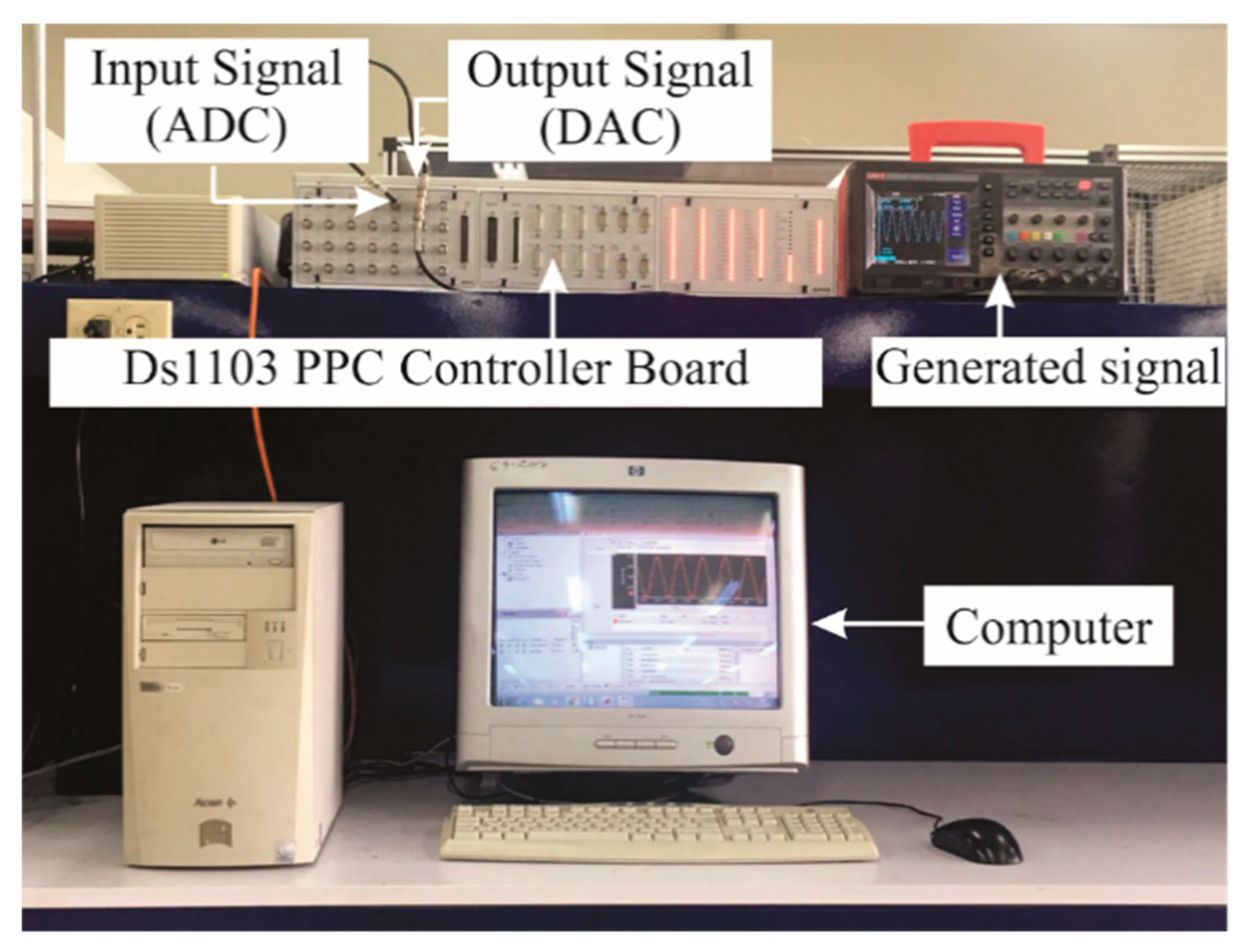
4. Experimentation and Results

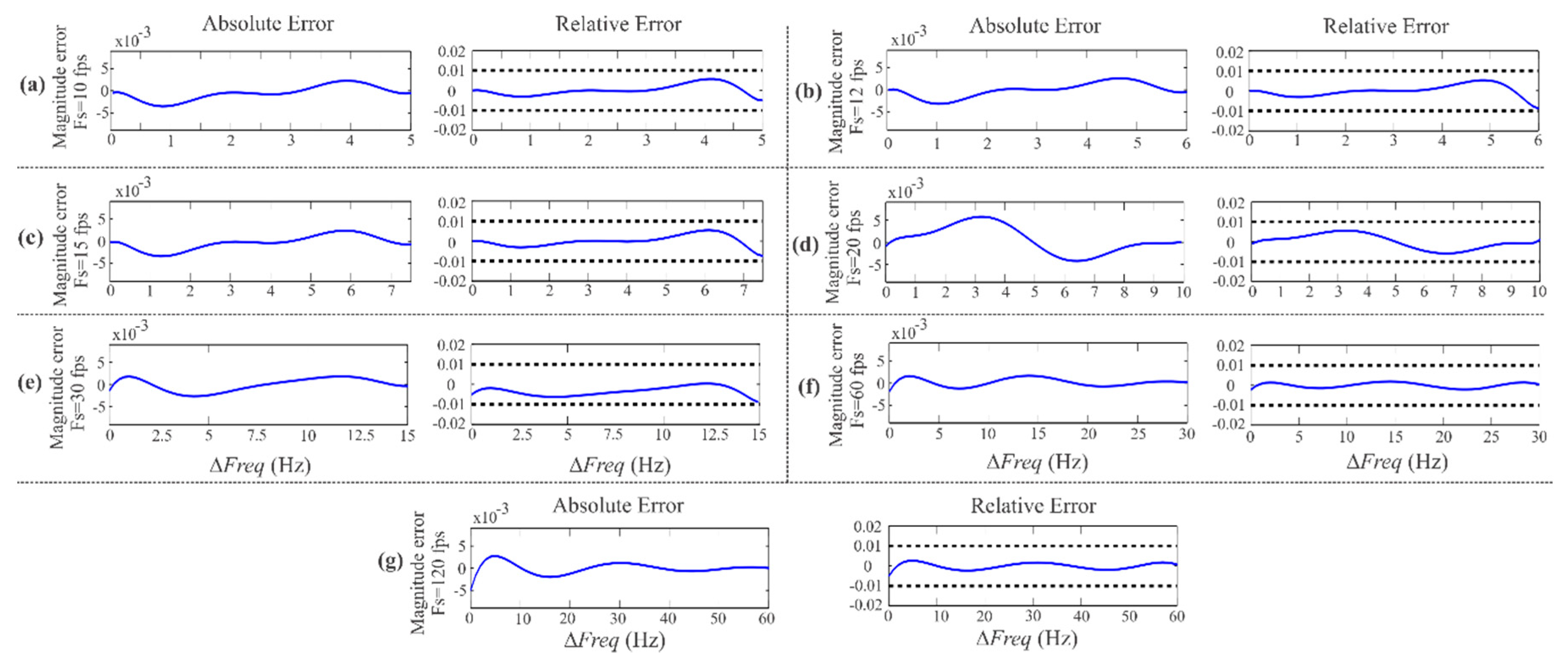
The obtained adjustment model and the results for the tests of validation are presented in this section. The validation is carried out using synthetic signals in software and through a real time simulator.

4.1. Model Results

Using the proposed methodology, the resulting model is a polynomial function of sixth and fourth orders for x and y, respectively. Therefore, it is given by:

$$\begin{array}{cc}{M}_{FIT}& =C_{0,0}+C_{1,0}x+C_{2,0}{x}^2+C_{3,0}{x}^3+C_{4,0}{x}^4+C_{5,0}{x}^5+C_{0,1}y+C_{0,2}{y}^2+C_{0,3}{y}^3\\ & +C_{0,4}{y}^4+C_{0,6}{y}^6+C_{1,1}xy+C_{2,1}{x}^{2}y+C_{3,1}{x}^{3}y+C_{4,1}{x}^{4}y+C_{5,1}{x}^{5}y+C_{1,2}x{y}^2\\ & +C_{2,2}{x}^2{y}^2+C_{3,2}{x}^3{y}^2+C_{4,2}{x}^4{y}^2+C_{1,3}x{y}^3+C_{2,3}{x}^2{y}^3+C_{3,3}{x}^3{y}^3+C_{1,4}x{y}^4\\ & +C_{2,4}{x}^2{y}^4,\end{array}$$

(11)

where the obtained coefficients using the proposed methodology are shown in

Table 2. Coefficients for the proposed model.

Coefficients
C0,0 = 0	C5,0 = 2.20676 × 10−7	C0,6 = −1.4120 × 10−9	C5,1 = 2.10556 × 10−10	C1,3 = 2.15466 × 10−6
C1,0 = −6.0525 × 10−2	C0,1 = 3.7635 × 10−4	C1,1 = 6.66086 × 10−3	C1,2 = −1.86745 × 10−4	C2,3 = 1.50529 × 10−7
C2,0 = −3.28595 × 10−3	C0,2 = −6.57461 × 10−5	C2,1 = 1.83899 × 10−4	C2,2 = −1.04144 × 10−5	C3,3 = −5.62059 × 10−12
C30 = 3.4396 × 10−4	C0,3 = 1.2709 × 10−6	C3,1 = −9.29113 × 10−7	C3,2 = 2.05616 × 10−8	C1,4 = −8.33054 × 10−9
C4,0 = −1.5051 × 10−4	C0,4 = −6.51693 × 10−9	C4,1 = 2.07606 × 10−8	C4,2 = −3.06276 × 10−10	C2,4 = −6.75353 × 10−10

. The order model is defined using as criterion that the terms less than 1 × 10⁻¹³ were omitted due to they do not affect considerably the estimation error.

The graphical representation of the proposed model is depicted in Figure 3a, where the ∆Freq is on the x-axis, the y-axis represents Fs and the z-axis is the magnitude.

From this plot, it can be observed that, for all cases of Fs, the 3D surface model fits well in a wide frequency range. Figure 3b shows the absolute errors which are computed by using:

$$E_{ABSOLUTE}=X_{FIT}-X_{IDEAL},$$

(12)

where X_FIT represents the obtained data using the proposed model and X_IDEAL denotes the reference data for each Fs. It can be noticed that the errors between the proposed model and the reference data are very small as they do not exceed 0.05 dB in the frequency range of interest.

In order to have a clearer view of these values, Figure 4 shows the errors independently. Also, having in mind that the IEEE Std. C37.118.1 presents the TVE as an important parameter to quantify the error in the measurement, it is observed that the TVE, calculated using (5), can also be estimated as a relative error if both the phase angle error and X_MEAS = X_FIT are zero. In this way, the relative error is given by:

$$E_{RELATIVE}=\frac{\left(X_{FIT}-X_{IDEAL}\right)}{\left(X_{IDEAL}\right)}\ast 100\%.$$

(13)

The Std. indicates that the TVE should not exceed 1%, which can be achieved by an error in magnitude of 1% [6]. For this reason, the relative error values are also depicted in Figure 4, as they can be directly compared with the TVE allowed by the Std. It is worth noting that other parameters used to verify the compliance with the Std., such as frequency error and rate-of-change-of-frequency error, are not presented because of two reasons—(i) the used phasor estimator algorithm is the one provided by the Std., that is, its performance requirements have been already verified by the Std. and (ii) the proposal, located after the phasor estimator, is an additional stage within the PMU, which aims to compensate magnitude to reduce the TVE under wide frequency deviations.

The polynomial orders in (11) are those that satisfy the aforementioned error upper bounds. Figure 4 shows the results of using a frequency range of Fs/2 for the seven Fs values, that is, 10, 12, 15, 20, 30, 60 and 120 fps. For example, Figure 4a shows the first case, Fs = 10 fps, with a frequency deviation of Fs/2 = 5 Hz. On the left side of Figure 4a, the magnitude of the absolute error, estimated using (12), is presented. This shows that the error is not greater than 0.005%, indicating that both the model data and the reference data are remarkably similar. On the right side of Figure 4a, the relative error obtained using (13) is depicted. The two black dotted lines represent the maximum allowable error-limits set by the Std., that is a maximum error value of 0.01% represents a TVE of 1%. Therefore, the relative error does not exceed these limits. Similar results are observed for the remaining of Fs values, see Figure 4b–g.

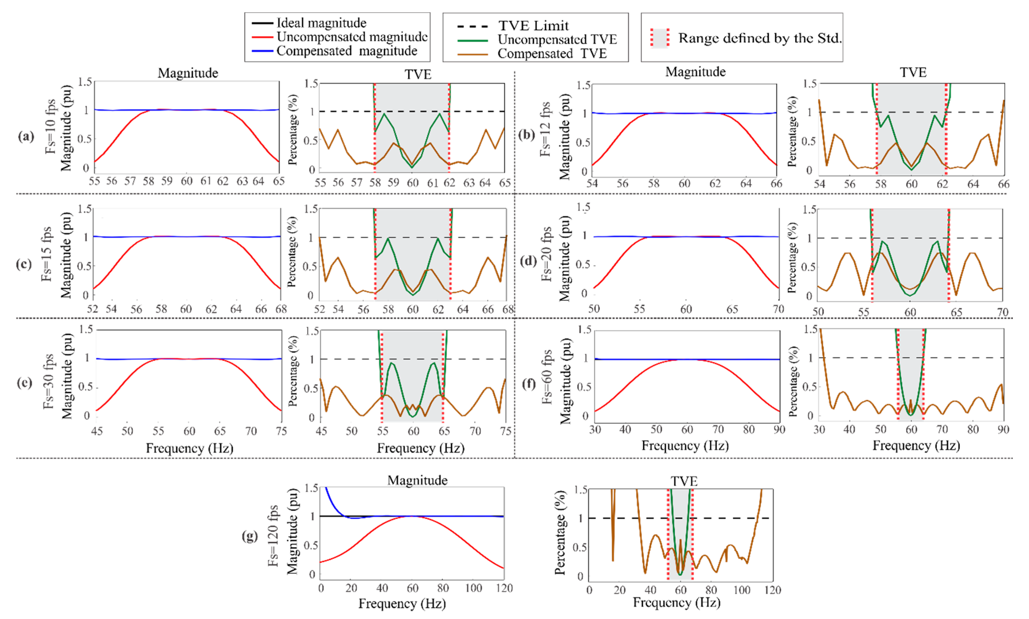
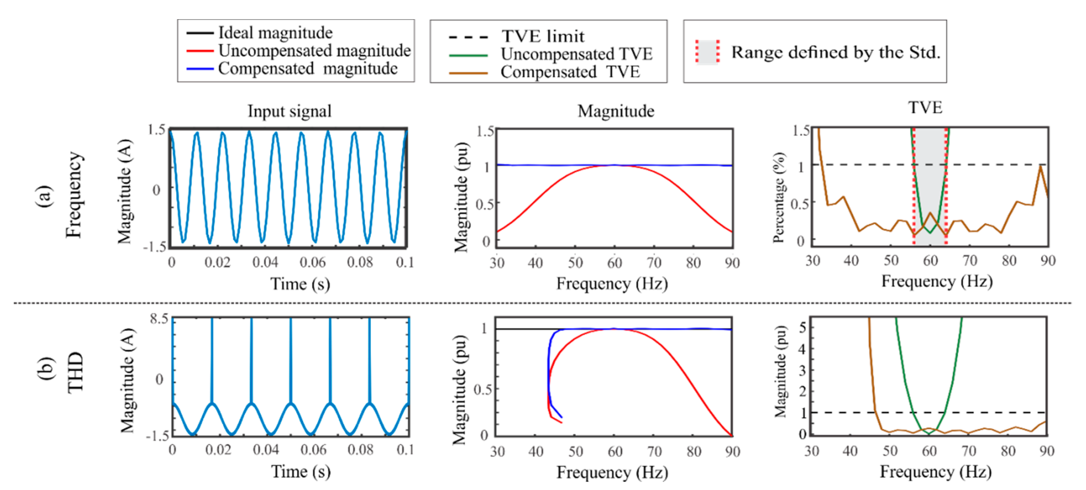
4.2. Steady-State Test

In order to show the proposal compliance with the Std., the recommended tests using the parameters presented in Table 1 for steady state tests are carried out. Figure 5 shows the obtained results for different values of Fs. There, sinusoidal signals with constant value of magnitude at different frequencies in steady state are used. Note that the frequency deviation range changes according to the values presented in Table 1. In general, two kinds of results, magnitude and TVE, can be observed in Figure 5 for each reporting rate. The magnitude results depict the magnitude values obtained by using uncompensated and compensated M-class filters. Likewise, the TVE results corresponds to compensated and uncompensated M-class filters. For example, Figure 5a shows, on the left side, the magnitude results and, on the right side, the TVE values for Fs = 10 fps. In the magnitude results, the ideal, uncompensated and compensated magnitudes are depicted using black, red and blue colors, respectively. In the TVE results, the errors due to the previous magnitude results are observed. The maximum allowable limit of TVE (1%) is denoted by a dotted black line. The green and brown colors denote the TVE results for uncompensated and compensated magnitudes, respectively. The gray area represents the frequency deviation range considered by the Std. For example, the Std. indicates a ∆Freq = Fs/5 for 10 ≤ Fs < 25 (see Table 1), therefore ∆Freq is equal to 2 Hz for Fs = 10 fps by encompassing a range from 58 to 62 Hz (see the plot on the right side of Figure 5a). In general, it can be observed that the obtained results, using the uncompensated M-class filter (given by the Std.), barely satisfy the allowable limits. On the contrary, the proposal (compensated results) greatly enhances the frequency range that can be compensated as it passes, for example, from ±2 Hz to ±5 Hz for Fs = 10 fps. This represents a noticeable advantage over the filter proposed by the Std. Similar results are found for other values of Fs (Figure 5b–g). It is worth noting that the maximum ∆Freq considered by the Std. is ±5 Hz, which applies for Fs = 30, 60 and 120 fps, according to the values presented in Table 1.

It can be observed that the proposal can compensate for a wider range of frequency deviations (see Figure 5e–g). In this regard, these results show that the proposal can deal with signals that present large frequency deviations using any of the Fs values considered in the Std.

Table 3. Frequency deviation ranges for the steady-state test.

Reporting Rate (fps)	10	12	15	20	30	60	120
Range established by the IEEE Std. C37.118.1 (Hz)	±2	±2.4	±3	±4	±5	±5	±5
Range with the proposal (Hz)	±5	±6	±8	±10	±15	±30	+60, −23

shows the ranges established by the IEEE Std. C37.118.1, which depends on the reporting rate and the ranges that can be compensated with the proposal. For all the reporting rates, the compensated ranges exceed the ones established by the Std. In fact, for a reporting rate of 60 fps, a range of ±30 Hz (from 30 to 90 Hz) is achieved, overcoming other reported works.

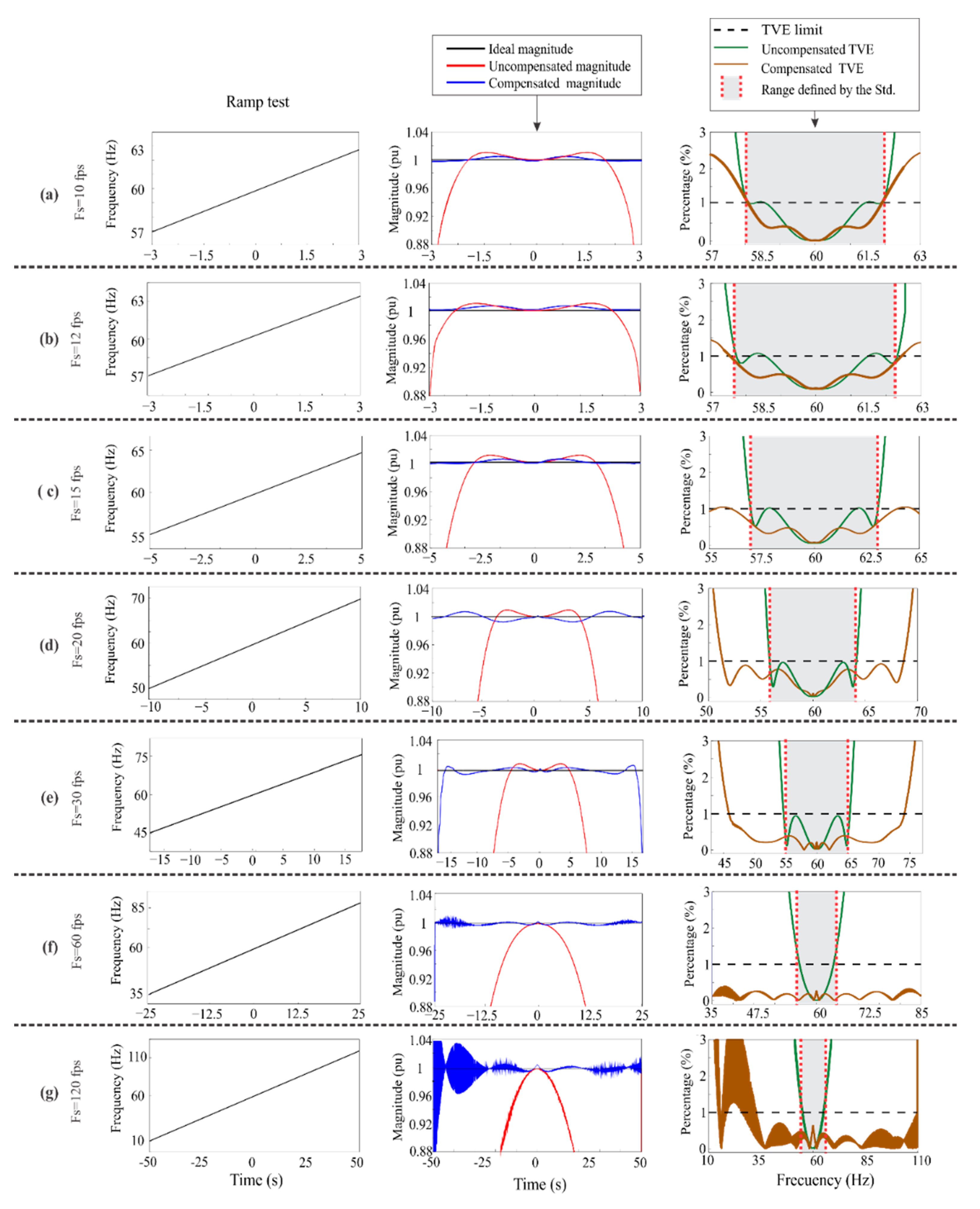
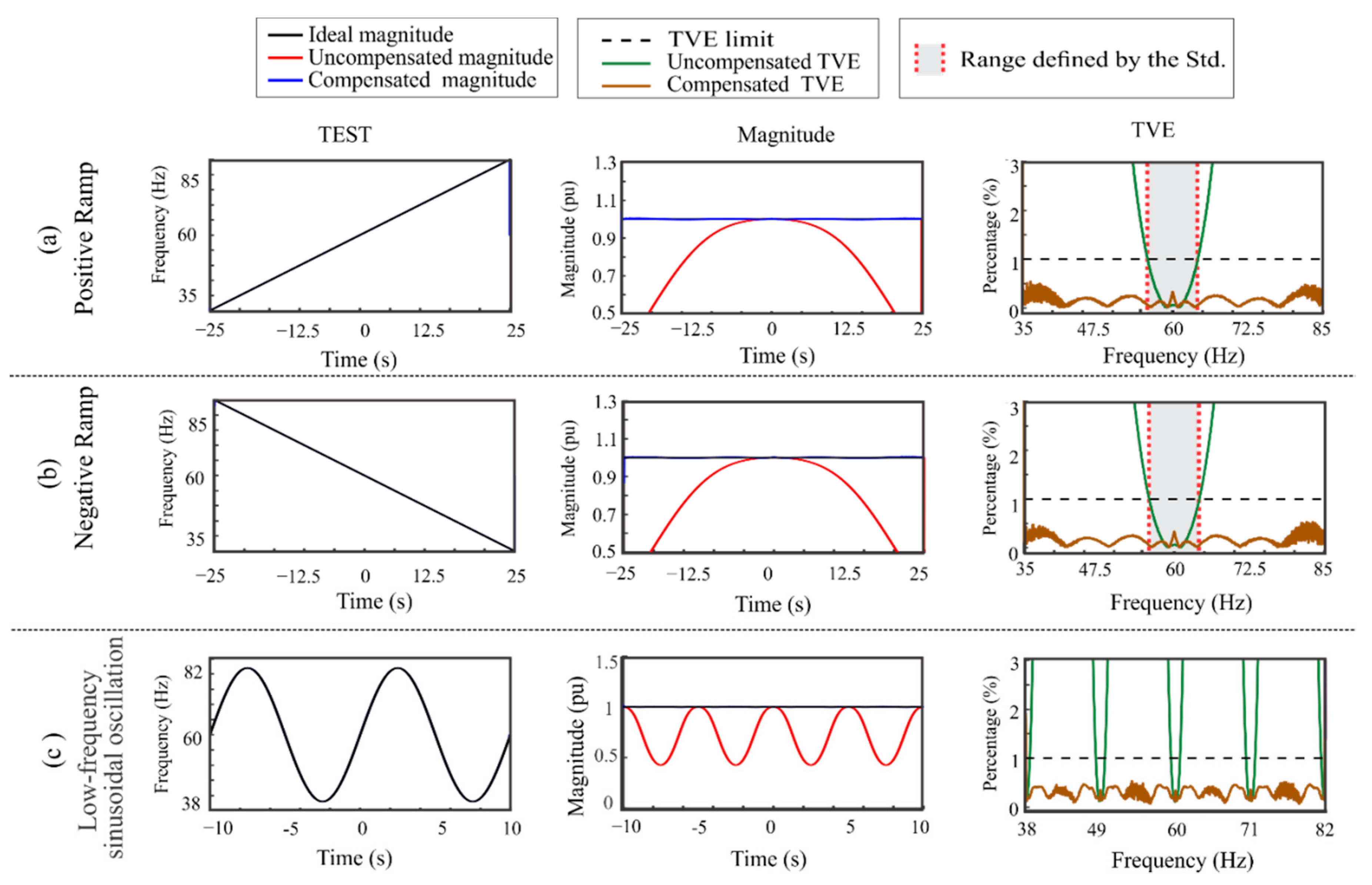
4.3. Dynamic Test: Linear Frequency Ramp

Figure 6 depicts the dynamic test results for the values of Fs shown in Table 1. The dynamic test proposed by the IEEE Std. C37.118.1 considers a linear frequency ramp with a positive slope of 1 Hz/s [6]. The frequency range depends on the value of Fs (see Table 1), for example, a frequency range from 56 to 64 Hz is considered for Fs = 20 fps, since ±Fs/5 = ±4 Hz. In Figure 6a, the case of Fs = 10 fps is presented. There, the plot on the left side presents the frequency values used for the ramp test, which is set to Fs/5 (±2 Hz). The plot in the middle shows the magnitude results, where the ideal, uncompensated and compensated magnitudes are depicted in black, red and blue colors, respectively. Although the uncompensated magnitude is close to the ideal one in the valid range, it has significant fluctuations that directly affect the TVE value. Furthermore, the plot on the right side describes the TVE values obtained for the ramp test, where the maximum allowable limit of TVE is denoted by a dotted black line. This plot shows that both the Std. and the proposal are valid in the same range (±2 Hz) (shown in the gray area). Despite having a similar range, the proposal presents for most of the frequency values a lower TVE than the one obtained by the uncompensated algorithm, for example, in Figure 6a, the uncompensated TVE for a time of 1.5 s is close to the allowable limit (1%), whereas the compensated TVE is close to 0.5%. Regarding the case of Fs = 12 fps, Figure 6b shows the range of TVE set by the Std. is ±2 1/3 Hz (gray area), which is exceeded by the proposal with a range of ±2.5 Hz. In the same regard, the case of Fs = 15 fps shows that the range of the Std. (±3 Hz) is exceeded by the proposal since it can deal with a range of ±4 Hz (Figure 6c). The remaining cases of Fs, 20, 30, 60 and 120 fps, are also presented in Figure 6d–g, respectively, where the Std. sets a valid range of ±5 Hz (gray areas). In these cases, the proposal achieves frequency ranges of ±8.5, ±14, ±26 and 27 to 50 Hz, respectively.

From the above-mentioned results, it is observed that the proposed model allows improvements in the magnitude compensation under dynamic frequency deviations even for the lowest value of Fs, that is, Fs = 10 fps, which is a difficult task due to the small available bandwidth (Fs/2). Besides that, it is also noticed that the range of ∆Freq that the proposed model can compensate depends on the available bandwidth of Fs, having a range of compensation from 27 to 50 Hz for an Fs of 120 fps. Therefore, the higher Fs value, the wider will be the range of frequency deviations that the model can compensate.

Table 4. Frequency deviation ranges for the dynamic test.

Reporting Rate (fps)	10	12	15	20	30	60	120
Range established by the IEEE Std. C37.118.1 (Hz)	±2	±2.3	±3	±4	±5	±5	±5
Range with the proposal (Hz)	±2	±2.5	±4	±8.5	±14	±26	35 to 100

shows the ranges established by the IEEE Std. C37.118.1 and the ranges that can be compensated by the proposal, which depends on the reporting rate. For all the Fs values, the results of Figure 6 in the third column show that the proposal generates lower TVE values (lines in brown color).

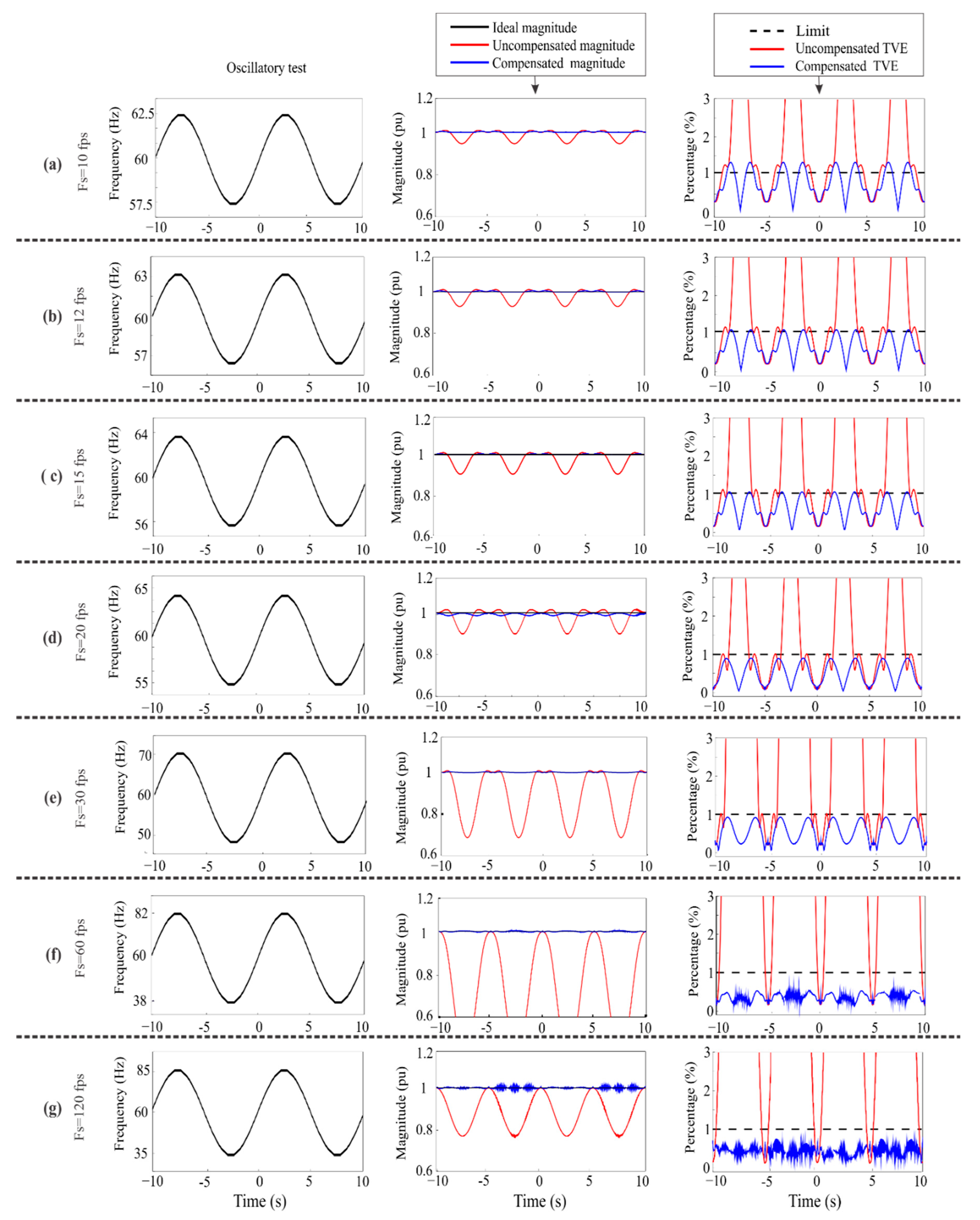
4.4. Dynamic Test: Sinusoidal Frequency Variation

Figure 7 shows the results of the sinusoidal frequency variation test. As above-mentioned, the IEEE Std. C37.118.1 does not present information for this test, however, it is considered in this work since it represents a possible condition in power systems. In this regard, the tests are constructed using (7), taking similar values of A_f to the ones taken by ∆Freq in the tests of linear frequency ramp. Therefore, the values of A_f for Fs equal to 10, 12, 15, 20, 30, 60 and 120 fps are 2.5, 3, 4, 5, 10, 22 and 25 Hz, respectively. For all the Fs values, f_f is set to 0.1 Hz, where two periods are considered. It is worth noting that the goal of these tests is to show the capabilities of the proposal for compensating magnitude under wide frequency deviations, even for sinusoidal frequency variations. In Figure 7a, the case of Fs = 10 fps is presented. There, the plot on the left side presents the frequency values used for the oscillatory test. The plot in the middle shows the magnitude results, where the ideal, uncompensated and compensated magnitudes are depicted in black, red and blue colors, respectively. Although the uncompensated magnitude is close to the ideal one in a small range, it deteriorates its accuracy as the frequency deviation increases. Similar to the previous study case (Section 4.3), the plot on the right side describes the TVE values obtained, where it can be observed that the frequency deviation range that the proposal can compensate increases along with the increment of Fs.

For instance, Figure 7c shows that the TVE is not exceeded for a ∆Freq = ±4 with an Fs = 15 fps, whereas Figure 7g shows that the TVE is not exceeded for a ∆Freq = ±25 with an Fs=120 fps. Periodical results of magnitude and TVE are observed due to the inherent periodicity of the sinusoidal oscillation. It is important to mention that the Std. does not establish a TVE limit for this test; yet, the 1% TVE limit is used. Although some values for the compensated TVE (blue color in Figure 7) exceed the 1%, they are better than the ones obtained for the uncompensated TVE, demonstrating the usefulness of the proposal. In fact, for higher reporting rates, the TVE values are kept below the 1% limit. In general, results demonstrate that the proposed compensation model for M-class PMUs can compensate the magnitude under wide frequency deviations, even if they are sinusoidal variations. Therefore, the power system applications that depend on the accuracy of the magnitude measurement may avoid to be adversely affected under wide frequency deviations.

4.5. Signals in a Real Time Digital Simulator (RTD)

In order to validate the proposal under a more realistic scenario, signals in a real-time digital simulator are implemented. Figure 8 shows the experimental setup. It consists of a computer to specify the signals using the mathematical models⁹ and a DS1103 PPC Controller Board from dSPACE. This board is a single-board system with a real-time processor PPC 750GX, 16-bit ADCs with a ±5 mV offset error and ±0.25% gain error and 16-bit DACs with ±1 mV offset error and ±0.5% gain error. The board generates the signal under analysis using a DAC (digital-analog-converter) and acquires the generated signal using an ADC (analog-digital-converter).

In Figure 9a, the results for the frequency tests in steady-state are shown, where the reporting rate of only 60 fps is used. Other reporting rates are tested in the previous section. The first column is an example of one generated signal. The second column presents the magnitude results where it is observed that the proposal can compensate for a wider frequency range (from 30 to 90 Hz). The third column shows the TVE values that confirm the wide compensation range. Similarly, Figure 9b shows the results for the harmonic distortion test, where 10% of each harmonic up to the 50th is used as stated in the Std. The harmonic distortion test is included to consider possible harmonic content into the power network. TVE results show that a range from 47.5 to 90 Hz can be compensated (third column), demonstrating the effectiveness of the proposal. The grey area is not shown in the third column of Figure 9b since the Std. does not consider the frequency deviation and the harmonic distortion in a combined way; however, it is evident that the proposal increases the range where the TVE value is acceptable.

Figure 10 shows the obtained results for dynamic scenarios, where ramp frequency tests (positive and negative) and a low-frequency sinusoidal oscillation test are carried out.

For the ramp tests, a ±25 Hz range of frequency deviation is correctly compensated, increasing the range defined by the Std. (gray area in the third column). On the other hand, in the sinusoidal frequency variation test (see Figure 10c), results indicate that the proposal can compensate the magnitude and, therefore, keep the TVE values within the acceptable limits (line in brown color, third column).

4.6. Comparison for M-Class Algorithms

Table 5. M-class algorithm comparison.

	Amplitude Step Test	Phase Step Test	Frequency Deviation Steady-State Test	Positive Ramp Test	Negative Ramp Test	IEEE Std. C37.118.1: Fs/RT limit/TVE limit	Frequency Range
Algorithm M-Class	Response Time [ms]	Response Time [ms]	TVE [%]	TVE [%]	TVE [%]
Complex filters [4]	49	58	2.6 × 10−5	0.0953	0.0953	60 fps 79 ms 1%	60 ±5 Hz
Adaptive extended Kalman Filtering [8]	65.1	17.85	0	NR	NR	60 fps 79 ms 1%	60 ±15 Hz
Second-order Taylor [23]	32	37	0.123	0.021	NR	50 fps 199 ms 1%	50 ±5 Hz
Empirical wavelet transform [24]	17.8	17.8	9.7 × 10−4	1.4 × 10−4	NR	50 fps 199 ms 1%	50 ±5 Hz
Interpolated DFT and Taylor Fourier Transform [25]	NR	NR	0.01	0.02	0.02	50 fps 199 ms 1%	50 ±5 Hz
Improved Taylor weighted least square [26]	52	32	1.1 × 10−5	0.003	0.003	100 fps 50 ms 1%	50 ±5 Hz
Real value Taylor weighted least square [26]	84	39	1.158	1.156	1.156	100 fps 50 ms 1%	50 ±5 Hz
DFT-based demodulation [26]	70	37	0.064	0.074	0.074	100 fps 50 ms 1%	50 ±5 Hz
Frequency-tracking and fixed-filter [27]	29.97	NR	0.07	0.07	0.07	50 fps 199 ms 1%	50 ±5 Hz
Proposal	15	15	1	1	1	120 fps 35 ms 1%	60 +60, −23 Hz (steady-state test) and +40, −25 Hz (dynamic test)

NR = Not reported.

shows a numerical comparison of the accuracy and response time for the amplitude and phase step tests using the TVE criterion. Also, the seventh column shows the limits of response time (RT) and TVE for the Fs value reported; as can be observed, the values of response time and TVE presented for the different algorithms are in compliance with the IEEE Std. C37.118.1 since they are lower. Although all the algorithms satisfy the frequency range of operation, the proposal overcomes these limits, allowing the correct estimation of the phasor information for a wider frequency range. In particular, the proposal extends the frequency range from (±5) to (+60, −23) in steady-state tests and from (±5) to (+40, −25) in dynamic tests by considering a Fs of 120 fps.

5. Conclusions

PMUs are key elements in many applications of power systems; despite being robust and accurate equipment, undesirable electric conditions in voltage or current signals such as large frequency changes may degrade their performance. In this work, a polynomial model to compensate the error in the estimation of magnitude associated to frequency deviations in voltage or current signals is proposed. The model is focused on the M-class filters stated in the IEEE Std. C37.118.1. In general, the proposed methodology to obtain the model considers the following elements—the magnitude frequency responses of the M-class filters at different reporting rates, a dilatation operation for normalizing the frequency ranges, a conversion to dB for a better amplitude representation and a fitting of a 3D function. This last function involves the magnitude, the frequency deviation and the reporting rate. As a result of the proposed methodology, a polynomial model with two independent variables is obtained. In other words, the output of the proposed model provides the compensation factors of magnitude by considering both the frequency deviation and the reporting rate, where all the reporting rates are considered since the Std. indicates that they have to be user selectable. The obtained results in the frequency tests for steady-state and dynamic conditions such as linear frequency ramps and sinusoidal frequency variation show that the proposed model satisfies the IEEE Std. C37.118.1 requirements and provides a far wider range, up to twenty times the range established by the Std. in dynamic conditions and higher than twelve times in steady-state conditions, where the relative error does not exceed 1%.

In future work, the phasor signal processing scheme provided by the IEEE Std. C37.118.1 along with the proposed model will be implemented into a field-programmable gate array (FPGA) platform in order to offer a system-on-a-chip solution for applications of PMUs, mainly those applications that are subjected to large frequency deviations in voltage or current signals such as start-up and shut-down of generators, in a frequency-controlled power electronic devices and clocks, protections and evaluation of system state based on frequency index, among others. It is important to mention that the methodology used to find the compensation model for M-class filters could be also applied to other demodulation filters in order to improve their performance under wide frequency deviations.

References

1. Roscoe, A.J.; Abdulhadi, I.F.; Burt, G.M. P and M class phasor measurement unit algorithms using adaptive cascaded filters. IEEE Trans. Power Deliv. 2013, 28, 1447–1459. [Google Scholar] [CrossRef] [Green Version]
2. Lee, H.; Cui, B.; Mallikeswaran, A.; Banerjee, P.; Srivastava, A.K. A review of synchrophasor applications in smart electric grid. Wiley Interdiscip. Rev. Energy Environ. 2017, 6, e223. [Google Scholar] [CrossRef]
3. Grigoraș, G.; Neagu, B.-C.; Gavrilaș, M.; Triștiu, I.; Bulac, C. Optimal Phase Load Balancing in Low Voltage Distribution Networks Using a Smart Meter Data-Based Algorithm. Mathematics 2020, 8, 549. [Google Scholar] [CrossRef] [Green Version]
4. Razo-Hernandez, J.R.; Mejia-Barron, A.; Granados-Lieberman, D.; Valtierra-Rodriguez, M.; Gomez-Aguilar, J.F. A New Phasor Estimator for PMU Applications: P Class and M Class. J. Mod. Power Syst. Clean Energy 2020, 8, 55–66. [Google Scholar] [CrossRef]
5. Granados-Lieberman, D. Global Harmonic Parameters for Estimation of Power Quality Indices: An Approach for PMUs. Energies 2020, 13, 2337. [Google Scholar] [CrossRef]
6. Power, I.; Society, E. C37.118.1-2011—IEEE Standard for Synchrophasor Measurements for Power Systems; IEEE: Piscataway, NJ, USA, 2011. [Google Scholar]
7. Srivastava, A.; Biswas, S. Synchrophasor Device Testing and Related Standards. In Smart Grid Handbook; John Wiley & Sons, Ltd.: Chichester, UK, 2016; pp. 1–24. [Google Scholar]
8. Kamwa, I.; Samantaray, S.R.; Joos, G. Wide frequency range adaptive phasor and frequency PMU algorithms. IEEE Trans. Smart Grid 2014, 5, 569–579. [Google Scholar] [CrossRef]
9. Georgilakis, P.S. Technical challenges associated with the integration of wind power into power systems. Renew. Sustain. Energy Rev. 2008, 12, 852–863. [Google Scholar] [CrossRef] [Green Version]
10. Granados-Lieberman, D.; Valtierra-Rodriguez, M.; Morales-Hernandez, L.; Romero-Troncoso, R.; Osornio-Rios, R. A Hilbert Transform-Based Smart Sensor for Detection, Classification, and Quantification of Power Quality Disturbances. Sensors 2013, 13, 5507–5527. [Google Scholar] [CrossRef] [Green Version]
11. Nanda, S.; Dash, P.K.; Chakravorti, T.; Hasan, S. A quadratic polynomial signal model and fuzzy adaptive filter for frequency and parameter estimation of nonstationary power signals. Meas. J. Int. Meas. Confed. 2016, 87, 274–293. [Google Scholar] [CrossRef]
12. Ferrero, A. Measuring electric power quality: Problems and perspectives. Meas. J. Int. Meas. Confed. 2008, 41, 121–129. [Google Scholar] [CrossRef]
13. Kušljević, M.D.; Tomić, J.J.; Marčetić, D.P. Active power measurement algorithm for power system signals under non-sinusoidal conditions and wide-range frequency deviations. IET Gener. Transm. Distrib. 2009, 3, 57–65. [Google Scholar] [CrossRef]
14. Chang, Y.; Liu, R.; Ba, Y.; Li, W. A New Control Logic for a Wind-Area on the Balancing Authority Area Control Error Limit Standard for Load Frequency Control. Energies 2018, 11, 121. [Google Scholar] [CrossRef] [Green Version]
15. Giray, M.M.; Sachdev, M.S. Off-Nominal Frequency Measurements in Electric power systems. IEEE Power Eng. Rev. 1989, 9, 42–43. [Google Scholar] [CrossRef]
16. Kundu, P.; Pradhan, A.K. Wide area measurement based protection support during power swing. Int. J. Electr. Power Energy Syst. 2014, 63, 546–554. [Google Scholar] [CrossRef]
17. Guan, M.; Pan, W.; Zhang, J.; Hao, Q.; Cheng, J.; Zheng, X. Synchronous Generator Emulation Control Strategy for Voltage Source Converter (VSC) Stations. IEEE Trans. Power Syst. 2015, 30, 3093–3101. [Google Scholar] [CrossRef]
18. Kamwa, I.; Samantaray, S.R.; Joos, G. Compliance analysis of PMU algorithms and devices for wide-area stabilizing control of large power systems. IEEE Trans. Power Syst. 2013, 28, 1766–1778. [Google Scholar] [CrossRef]
19. Cuesta, A.; Gomez-Gil, F.; Fraile, J.; Rodríguez, J.; Calvo, J.; Vara, J. Feasibility of a Simple Small Wind Turbine with Variable-Speed Regulation Made of Commercial Components. Energies 2013, 6, 3373–3391. [Google Scholar] [CrossRef] [Green Version]
20. Silva, R.P.M.; Delbem, A.C.B.; Coury, D.V. Genetic algorithms applied to phasor estimation and frequency tracking in PMU development. Int. J. Electr. Power Energy Syst. 2013, 44, 921–929. [Google Scholar] [CrossRef]
21. Sa-ngawong, N.; Ngamroo, I. Intelligent photovoltaic farms for robust frequency stabilization in multi-area interconnected power system based on PSO-based optimal Sugeno fuzzy logic control. Renew. Energy 2015, 74, 555–567. [Google Scholar] [CrossRef]
22. Chakir, M.; Kamwa, I.; Le Huy, H. Extended C37.118.1 PMU algorithms for joint tracking of fundamental and harmonic phasors in stressed power systems and microgrids. IEEE Trans. Power Deliv. 2014, 29, 1465–1480. [Google Scholar] [CrossRef]
23. Bi, T.; Liu, H.; Feng, Q.; Qian, C.; Liu, Y. Dynamic phasor model-based synchrophasor estimation algorithm for M-class PMU. IEEE Trans. Power Deliv. 2015, 30, 1162–1171. [Google Scholar] [CrossRef]
24. Chauhan, K.; Reddy, M.V.; Sodhi, R. A novel distribution-level phasor estimation algorithm using empirical wavelet transform. IEEE Trans. Ind. Electr. 2018, 65, 7984–7995. [Google Scholar] [CrossRef]
25. Tosato, P.; Macii, D.; Luiso, M.; Brunelli, D.; Gallo, D.; Landi, C. A Tuned Lightweight Estimation Algorithm for Low-Cost Phasor Measurement Units. IEEE Trans. Instrum. Meas. 2018, 67, 1047–1057. [Google Scholar] [CrossRef]
26. Xu, S.; Liu, H.; Bi, T.; Martin, K.E. An improved Taylor weighted least squares method for estimating synchrophasor. Int. J. Electr, Power Energy Syst. 2020, 120, 105987. [Google Scholar] [CrossRef]
27. Roscoe, A.J. Exploring the relative performance of frequency-tracking and fixed-filter phasor measurement unit algorithms under C37.118 test procedures, the effects of interharmonics, and initial attempts at merging P-Class response with M-Class filtering. IEEE Trans. Instrum. Meas. 2013, 62, 2140–2153. [Google Scholar] [CrossRef] [Green Version]
28. Phadke, A.G.; Kasztenny, B. Synchronized phasor and frequency measurement under transient conditions. IEEE Trans. Power Deliv. 2009, 24, 89–95. [Google Scholar] [CrossRef]
29. Warichet, J.; Sezi, T.; Maun, J.C. Considerations about synchrophasors measurement in dynamic system conditions. Int. J. Electr. Power Energy Syst. 2009, 31, 452–464. [Google Scholar] [CrossRef]
30. Ren, J.; Kezunovic, M.; Stenbakken, G. Characterizing dynamic behavior of PMUs using step signals. Eur. Trans. Electr. Power 2011, 21, 1496–1508. [Google Scholar] [CrossRef]
31. Gurusinghe, D.R.; Rajapakse, A.D.; Narendra, K. Testing and enhancement of the dynamic performance of a phasor measurement unit. IEEE Trans. Power Deliv. 2014, 29, 1551–1560. [Google Scholar] [CrossRef]
32. Castello, P.; Lixia, M.; Muscas, C.; Pegoraro, P.A. Impact of the model on the accuracy of synchrophasor measurement. IEEE Trans. Instrum. Meas. 2012, 61, 2179–2188. [Google Scholar] [CrossRef]
33. Shah, N.N.; Joshi, S.R. Utilization of DFIG-based wind model for robust damping of the low frequency oscillations in a single SG connected to an infinite bus. Int. Trans. Electr. Energy Syst. 2019, 29, e2761. [Google Scholar] [CrossRef]
34. Seo, W.S.; Kang, S.H.; Nam, S.R. Non-recursive Discrete Fourier Transform-Based Frequency Estimation of the Power System. J. Electr. Eng. Technol. 2019, 14, 1505–1515. [Google Scholar] [CrossRef]
35. Nam, S.-R.; Kang, S.-H.; Kang, S.-H. Real-Time Estimation of Power System Frequency Using a Three-Level Discrete Fourier Transform Method. Energies 2014, 8, 79–93. [Google Scholar] [CrossRef]
36. Bamigbade, A.; Khadkikar, V.; al Hosani, M.; Zeineldin, H.H.; el Moursi, M.S. Gain compensation approach for low-voltage ride-through and dynamic performance improvement of three-phase type-3 PLL. IET Power Electr. 2020, 13, 1613–1621. [Google Scholar] [CrossRef]
37. Razo-Hernandez, J.R.; Valtierra-Rodriguez, M.; Granados-Lieberman, D.; Tapia-Tinoco, G.; Rodriguez-Rodriguez, J.R. A phasor estimation algorithm based on Hilbert transform for P-class PMUs. Adv. Electr. Comput. Eng. 2018, 18, 97–104. [Google Scholar] [CrossRef]
38. Martin, K.E.; Hamai, D.; Adamiak, M.G.; Anderson, S.; Begovic, M.; Benmouyal, G.; Brunello, G.; Burger, J.; Cai, J.Y.; Dickerson, B.; et al. Exploring the IEEE standard C37.118-2005 synchrophasors for power systems. IEEE Trans. Power Deliv. 2008, 23, 1805–1811. [Google Scholar] [CrossRef]
39. Fan, D.; Centeno, V. Phasor-based synchronized frequency measurement in power systems. IEEE Trans. Power Deliv. 2007, 22, 2010–2016. [Google Scholar] [CrossRef]
40. Howlader, A.M.; Sadoyama, S.; Roose, L.R.; Chen, Y. Active power control to mitigate voltage and frequency deviations for the smart grid using smart PV inverters. Appl. Energy 2020, 258, 114000. [Google Scholar] [CrossRef]
41. Liu, X.; Laverty, D.M.; Best, R.J.; Li, K.; Morrow, D.J.; McLoone, S. Principal Component Analysis of Wide-Area Phasor Measurements for Islanding Detection—A Geometric View. IEEE Trans. Power Deliv. 2015, 30, 976–985. [Google Scholar] [CrossRef]
42. Samantaray, S.R.; Kamwa, I.; Joos, G. Phasor measurement unit based wide-area monitoring and information sharing between micro-grids. IET Gener. Transm. Distrib. 2017, 11, 1293–1302. [Google Scholar] [CrossRef]
43. Kamwa, I.; Pradhan, A.K.; Joos, G. Adaptive phasor and frequency-tracking schemes for wide-area protection and control. IEEE Trans. Power Deliv. 2011, 26, 744–753. [Google Scholar] [CrossRef]
44. Siti, M.W.; Tungadio, D.H.; Sun, Y.; Mbungu, N.T.; Tiako, R. Optimal frequency deviations control in microgrid interconnected systems. IET Renew. Power Gener. 2019, 13, 2376–2382. [Google Scholar] [CrossRef]
45. Marzebali, M.H.; Mazidi, M.; Mohiti, M. An adaptive droop-based control strategy for fuel cell-battery hybrid energy storage system to support primary frequency in stand-alone microgrids. J. Energy Storage 2020, 27, 101127. [Google Scholar] [CrossRef]
46. Cao, J.; Du, W.; Wang, H.; McCulloch, M. Optimal Sizing and Control Strategies for Hybrid Storage System as Limited by Grid Frequency Deviations. IEEE Trans. Power Syst. 2018, 33, 5486–5495. [Google Scholar] [CrossRef]
47. Liu, Y.; Du, W.; Xiao, L.; Wang, H.; Cao, J. A method for sizing energy storage system to increase wind penetration as limited by grid frequency deviations. IEEE Trans. Power Syst. 2016, 31, 729–737. [Google Scholar] [CrossRef]
48. Lay, D. Linear Algebra and Its Applications, 4th ed.; Pearson Education: Boston, MA, USA, 2012. [Google Scholar]
Figure 1. Phasor measurement unit (PMU): (a) Phasor signal processing algorithm for P-class PMU and (b) Proposed compensation for M-class PMU.
Mathematics 08 01361 g001
Figure 2. Proposed methodology: (a) Flowchart, (b) magnitude frequency response, (c) Dilated curves and (d) Zoom for 10, 12 and 15 dilated curves.
Mathematics 08 01361 g002
Figure 3. 3D fit results: (a) 3D surface and (b) Polynomial fit error.
Mathematics 08 01361 g003
Figure 4. Absolute and relative errors for: (a) 10 fps, (b) 12 fps, (c) 15 fps, (d) 20 fps, (e) 30 fps, (f) 60 fps and (g) 120 fps.
Mathematics 08 01361 g004
Figure 5. Magnitude and total vector error (TVE) results for steady-state test: (a) 10 fps, (b) 12 fps, (c) 15 fps, (d) 20 fps, (e) 30 fps, (f) 60 fps and (g) 120 fps.
Mathematics 08 01361 g005
Figure 6. Magnitude and TVE results for linear frequency ramp: (a) 10 fps, (b) 12 fps, (c) 15 fps, (d) 20 fps, (e) 30 fps, (f) 60 fps and (g) 120 fps.
Mathematics 08 01361 g006
Figure 7. Magnitude and TVE results for: (a) 10 fps, (b) 12 fps, (c) 15 fps, (d) 20 fps, (e) 30 fps, (f) 60 fps and (g) 120 fps.
Mathematics 08 01361 g007
Figure 8. Experimental setup using the real time digital simulator (RTD).
Mathematics 08 01361 g008
Figure 9. Experimental tests in steady-state: (a) Static changes frequency and (b) Harmonic distortion test.
Mathematics 08 01361 g009
Figure 10. Experimental tests in dynamic conditions: (a) positive ramp, (b) negative ramp and (c) sinusoidal frequency variation test.
Mathematics 08 01361 g010