Multi-Wavelets Galerkin Method for Solving the System of Volterra Integral Equations


1
Division of Computational Mathematics and Engineering, Institute for Computational Science, Ton Duc Thang University, Ho Chi Minh City 70000, Vietnam
2
Faculty of Mathematics and Statistics, Ton Duc Thang University, Ho Chi Minh City 70000, Vietnam
3
Department of Mathematics, College of Science, King Saud University, P.O. Box 2455, Riyadh 11451, Saudi Arabia
4
Institute of Computer Science, University of Tartu, 50090 Tartu, Estonia
*
Author to whom correspondence should be addressed.
Mathematics 2020, 8(8), 1369; https://0-doi-org.brum.beds.ac.uk/10.3390/math8081369
Submission received: 1 July 2020
/
Revised: 8 August 2020
/
Accepted: 12 August 2020
/
Published: 15 August 2020
(This article belongs to the Special Issue Differential/Difference Equations: Mathematical Modeling, Oscillation and Applications)
Abstract
:In this work, an efficient algorithm is proposed for solving the system of Volterra integral equations based on wavelet Galerkin method. This problem is reduced to a set of algebraic equations using the operational matrix of integration and wavelet transform matrix. For linear type, the computational effort decreases by thresholding. The convergence analysis of the proposed scheme has been investigated and it is shown that its convergence is of order , where J is the refinement level and r is the multiplicity of multi-wavelets. Several numerical tests are provided to illustrate the ability and efficiency of the method.
1. Introduction
In this paper, we study and construct a novel numerical algorithm for the system of Volterra integral equations of the second kind
where is a given real-valued continuous function, is the unknown function that will be determined and the function with is a given linear or nonlinear function of which satisfies the following Lipschitz condition with respect to the third variable: for all and for all ,
Therefore, the functions and are considered so that the Equation (1) has a unique solution.
Equation (1) is the general form of second-order Volterra integral equation and appears in scientific applications in chemistry, engineering, mathematics, and physics [1,2,3,4]. Numerical and analytical solutions of linear and nonlinear Volterra integral equations have been investigated in many papers. A useful method to solve such equations is the Adomian decomposition method. This method was used to investigate the existence and uniqueness of solutions of this type of equation [5,6]. One of the best paper which utilizes the multi-wavelets for solving integro-differential equations was presented by Saray [7]. In [7], an efficient algorithm was proposed for solving the Volterra integro-differential equation. This method outperforming former approaches. Golbabai et al. [8] developed a general method based on radial basis function networks to solve the system of Volterra integral equations. The modified homotopy perturbation method for solving this type of equation has been proposed by Aminikhah et al. [5,9]. Kılıçman et al. [10] used Simpson’s rule to solve this equation. Aguilar and Brunner used collocation techniques based on spline polynomials [11]. The umbral calculus and the Laplace transform methods were used as solution approaches as well [12].
Wavelets and specially multi-wavelets Galerkin method represent an efficient way to solve a variety of equations, including ordinary differential equations (ODEs), partial differential equations (PDEs), and integral equations [7,13,14]. Due to the discrete-time characterization of wavelet coefficient decay, the sparse form of the coefficients matrices arises. This property is very useful to reduce the computational cost. In this work, we aim to solve the system of the Volterra integral equation using Alpert’s multi-wavelets by exploiting the above-mentioned property. Some results are formally proved and supported by numerical experiments.
The paper is structured as follows. A brief introduction of the Alpert’s multi-wavelets is provided in Section 2. In Section 3, the wavelet Galerkin method is used to approximate the solution of the problem, and the convergence analysis is investigated. Some numerical experiments are performed to illustrate the efficiency and accuracy of the proposed method.
2. Alpert’s Multi-Wavelets and Multiresolution Analysis
Alpert et al. [13,15] introduced a class of multi-wavelets for , which are indexed by a parameter and built via Lagrange polynomials of degree less than r. These multi-wavelets are piecewise polynomials that are locally supported and orthonormal. The multiresolution analysis (MRA) framework, introduced and developed by Mallat [16] and Meyer [17], is useful to construct these bases.
According to MRA, a set of primal scaling functions is introduced for primal subspace . By translation and dilation of primal scaling functions , we determine a space ,
where and are the dilation and translation operators, respectively such that for a given function h, and , also for . Therefore, is a polynomial of degree less than k which is restricted to where and .
For a fixed integer , the orthogonal projection of onto is determined by
The coefficients are determined by [18,19,20]. To avoid computing integrals, the Gauss–Legendre Quadrature are applied as follows
where and are the Gauss-Legendre Quadrature weights and the roots of Legendre polynomial of order r, respectively which are introduced in [21,22,23]. The projection converges to h if the function (r times continuously differentiable) [15]. approximates h with mean error bounded as follows
Assume that , where . refers to the function vector called a multi-scaling function. In fact, is a function vector which includes the scaling function in the space . By this definition, one can rewrite (3) viz, where H is a vector with entries and has dimension .
This construction of multi-wavelets for can be extended to the two–dimensional space including . Let us introduce the space which is spanned by orthonormal bases Therefore, any function can be projected onto the by the projection via,
where H is an matrix whose elements are obtained by
where . By the following theorem, it is possible to bound the error for such projection, if the function h is sufficiently smooth.
Theorem 1
([15]). Suppose that the function has continuous partial derivatives of order r and mixed partial derivative of order . Then
where
As the subspaces are nested, there exist complementary orthogonal subspaces such that
here and in the following ⨁ denotes orthogonal sums. There is a family of other bases such that the dilations and translations of these bases span the complementary subspaces , namely,
The functions are called multi-wavelets. Due to (9), the multi-scale decomposition can be inductively found, . This decomposition gives rise to the multi-scale projection operator that maps onto via
where is the orthonormal projection operator that maps onto . In fact, by using multi-scale projection operator, any function can be approximated by multi-wavelets of higher levels , and the multi-scaling functions of the coarse space viz,
where
Note that the single-scale coefficients can be determined by (4). However, for evaluating the multi-wavelets coefficients of higher levels, in many cases, they have to be calculated numerically. To avoid such numerical computations, the wavelet transform matrix can be applied, as introduced in [14,24]. This matrix is useful to find the multi-wavelets by using the scaling functions
where and , . Using the vector function and (11), we can write
where is an N-dimensional vector with entries and for , and . Besides, it is obvious that .
Thresholding
Alpert’s multi-wavelets provide vanishing moments of order for , i.e.,
Furthermore, Alpert’s multi-wavelets are uniformly bounded concerning to and , i.e.,
The vanishing moments and normalization (16) imply that the detail coefficients become small when the underlying function is locally smooth. Therefore it is possible to obtain [25]
So the detail coefficients decay at the rate of and in the regions where the function is smooth, most of the detail coefficients may be discarded when the refinement level J increases. This gives rise to thresholding. The thresholding operator is introduced by
where and the elements of are defined by
Note that the thresholding affects only the detail coefficients while the coarse scale coefficients remain unchanged.
The approximation error due to the thresholding can be estimated similarly to the classical wavelets. Let be the approximation operator . The approximation error due to the thresholding can be bounded as stated by the following proposition [25].
Proposition 1.
(Approximation error). Let Ω be bounded and with . Then the approximation error concerning to the set of significant details is uniformly bounded concerning to , , i.e.,
for some constant independent of . Here and are the projections according to (11) corresponding to the coefficients and .
3. Multi-Wavelets Galerkin Method
In this section, we use the wavelet Galerkin method to solve the system of the Volterra integral Equation (1). To this end, we will apply the interpolation property of scaling functions to reach an efficient algorithm. Assume that the solution of Equation (1) can be expanded using multi-scale projection operator based on multi-wavelets as follows
where ⊗ is the Kronecker product and is a vector whose elements are n unknown sub-vectors with a dimension of such that
One can imagine two types of equations, linear and nonlinear. For the linear type, the i-th component of the vector function has the form
and it can be approximated by multi-scale operator, i.e.,
where are matrices. Integrating from 0 to x, we get
where are matrices and the rest are vectors. But if the j-th component of vector function is nonlinear, one can consider the following expansion
where is a vector whose elements are nonlinear algebraic equations. In view of the Equations (23) and (24), and using operational matrix of integration for multi-wavelets introduced in [7,14,15], one can write
with , and .
Such an approximation can be considered for the j-th element of viz,
and thus by putting we have
Now, we introduce the residual as
To apply the Galerkin method, it is necessary that . Thus we have
By solving this system of linear and nonlinear equations using restarted generalized minimal residual method (GMRES) and Newton methods, respectively, we obtain the approximate solution of the Equation (1). Note that because we use the Galerkin method with orthogonal bases, such a system will have a unique solution [26].
Convergence Analysis
Theorem 2.
Suppose thatwhereandare the exact and approximate solutions of nonlinear system (1), respectively. Let X be an open set inand letbe a function such thatfor anyand the condition (2) is satisfied. Furthermore, presume that. Furthermore, assume that the residualwhere the residualis specified as
andis introduced in (27).
where κ is a positive constant. Consequently,when.
Proof.
Using (27), (29) and the hypotheses of the theorem, we can write
where . Since the function satisfies the Lipschitz condition (2), Equation (30) can be reduced to
Now, suppose that
where and are the vectors and thus, one can write
Taking -norm from both sides and using the triangle inequality yields
where the second row comes from theorem 8 in [27]. Since Alpert multi-wavelets are orthonormal, one can write
According to the previous section, when has high vanishing moments and the function h is smooth, decays fast in . By means of vanishing moments of Alpert’s multi-wavelets and the matrix norms inequalities, we get
where . Now Equation (5) leads to the desired result
☐
Theorem 3.
Proof.
Taking as the approximate solution of (1) and as the approximate solution obtained from solving (28) using restarted GMRES or Newton methods, the convergence can be concluded from
The approximate solution of (1) satisfies
Let us consider where is the vector and thus, we have
Since Alpert multi-wavelets are orthonormal, one can write
Therefore one can bound the error of via
4. Numerical Examples
In this section, some numerical experiments are considered to illustrate the convergence and efficiency of the proposed method. To this end, we report the errors of the solution which is defined by
where u and are the exact and approximate solution of systems (1), respectively. In order to get the sparse coefficients matrix in the linear type, all the entries of this matrix that are less than a small positive number are set to zero. Finally, one can find the rate of sparsity which is defined by [28]
where is the total number of elements and the number of elements remaining after thresholding.
Example 1.
Example 2.
Let us consider the following system of Volterra integral equation as a further example
Example 3.
Let us consider the following nonlinear system
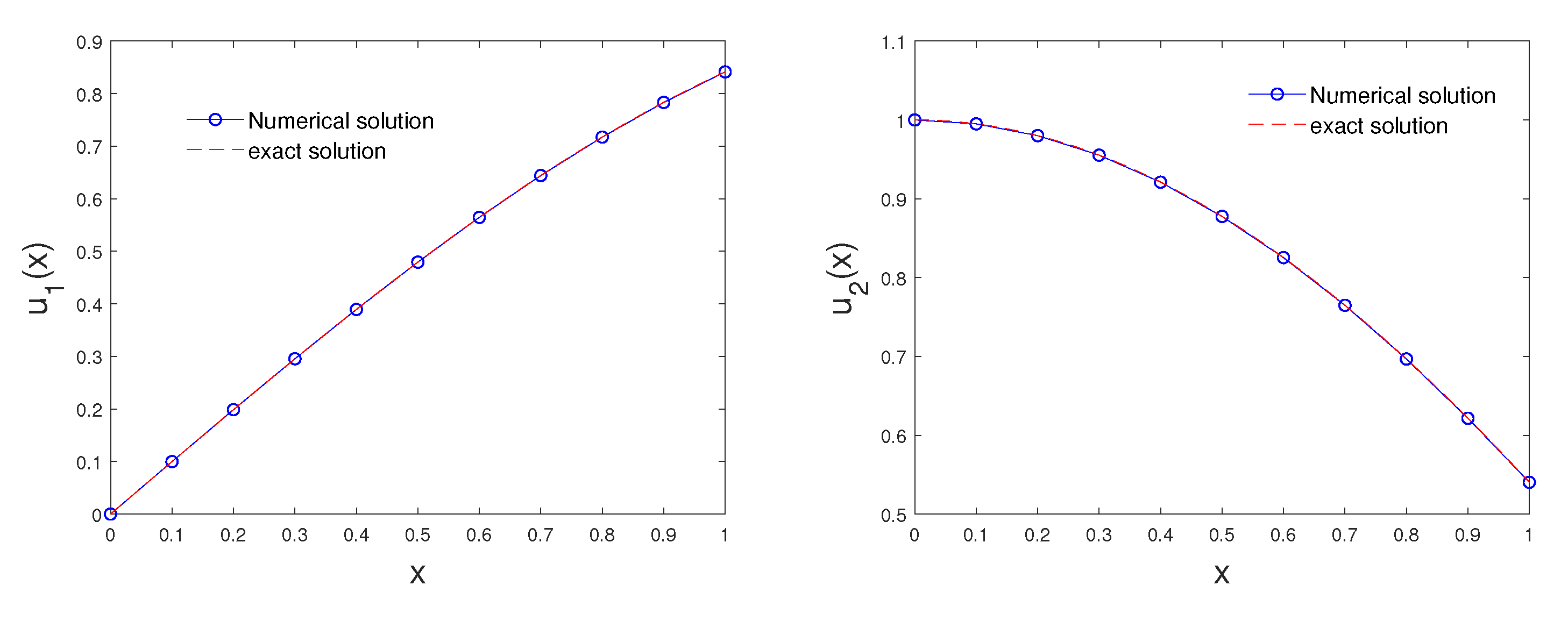
Table 2 is reported to show the efficiency and accuracy of the proposed method. We observe when the refinement level J and multiplicity parameter r increase, the L2-errors decrease. In Table 3 and Table 4, results are compared with other methods [10,31,32,33] in terms of the absolute errors. In this paper, J and r are the criteria for the discretization and the degree of polynomials used as a basis, respectively. Taking r = 7 and J = 2, the results of Table 3 and Table 4 indicate that the proposed method solves this equation better than others [10,31,32,33]. Furthermore, we reported the exact and numerical solution by Figure 5.
5. Conclusions
In this paper, we proposed the multi-wavelets Galerkin method to solve the linear and nonlinear Volterra integral equation. The convergence analysis and numerical simulations indicate that the proposed method gives a satisfactory approximation to the exact solution. Thresholding can be used to increase sparsity for a lower computational cost, without affecting the error in . Using the interpolation property of Alpert’s multi-wavelets, the proposed method turns out to be fast and very competitive against state-of-the-art techniques. The main advantages of the proposed method are the lower computational cost and lower complexity.
Author Contributions
Conceptualization, H.V.L. and H.B.J.; methodology, software, H.B.J. and S.T.; validation, formal analysis, H.B.J.; writing–original draft preparation, investigation, funding acquisition, H.V.L., H.B.J. and S.T.; writing–review and editing, H.V.L., H.B.J. and S.T. All authors have read and agreed to the published version of the manuscript.
Funding
This project was supported by Researchers Supporting Project number (RSP-2020/210), King Saud University, Riyadh, Saudi Arabia.
Conflicts of Interest
The authors declare no conflict of interest.
References
- Jerri, A. Introduction to Integral Equations with Applications; Wiley: New York, NY, USA, 1999. [Google Scholar]
- Li, Y.; Xu, R.; Lin, J. Global dynamics for a class of infection-age model with nonlinear incidence. Nonlinear Anal. Model. Control 2018, 24, 47–72. [Google Scholar] [CrossRef]
- Nordbo, A.; Wyller, J.; Einevoll, G.T. Neural network firing-rate models on integral form. Biol. Cybern. 2007, 97, 195–209. [Google Scholar] [CrossRef] [PubMed]
- Porter, D.; Stirling, D.S. Integral Equations: A Practical Treatment from Spectral Theory to Applications; Cambridge University Press: Cambridge, UK, 2004. [Google Scholar]
- Aminikhah, H.; Biazar, J. A new analytical method for solving systems of Volterra integral equations. Int. J. Comput. Math. 2010, 87, 1142–1157. [Google Scholar] [CrossRef]
- Biazar, J.; Babolian, E.; Islam, R. Solution of a system of Volterra integral equations of the first kind by Adomian method. Appl. Math. Comput. 2003, 139, 249–258. [Google Scholar]
- Saray, B.N. An efficient algorithm for solving Volterra integro-differential equations based on Alpert’s multi-wavelets Galerkin method. J. Comput. Appl. Math. 2019, 348, 453–465. [Google Scholar] [CrossRef]
- Golbabai, A.; Mammadova, M.; Seifollahi, S. Solving a system of nonlinear integral equations by an RBF network. Comput. Math. Appl. 2009, 57, 1651–1658. [Google Scholar]
- Saberi-Nadjafi, J.; Tamamgar, M. Modified homotopy perturbation method for solving the system of Volterra integral equations. Int. Nonlinear Sci. Numer. Simul. 2008, 9, 409–413. [Google Scholar] [CrossRef]
- Kılıçman, A.; Kargaran Dehkordi, L.; Tavassoli Kajani, M. Numerical Solution of Nonlinear Volterra Integral Equations System Using Simpson’s 3/8 Rule. Math. Prob. Eng. 2012, 2012, 1–16. [Google Scholar] [CrossRef]
- Aguilar, M.; Brunner, H. Collocation methods for second-order Volterra integrodifferential equations. Appl. Numer. Math. 1988, 4, 455–470. [Google Scholar] [CrossRef]
- Górska, K.; Horzela, A. The Volterra type equations related to the non-Debye relaxation. Commun. Nonlinear Sci. 2020, 85, 105246. [Google Scholar] [CrossRef]
- Alpert, B.; Beylkin, G.; Gines, D.; Vozovoi, L. Adaptive solution of partial differential equations in multiwavelet bases. J. Comput. Phys. 2002, 182, 149–190. [Google Scholar] [CrossRef] [Green Version]
- Saray, B.N.; Lakestani, M.; Razzaghi, M. Sparse representation of system of Fredholm integro-differential equations by using Alpert multiwavelets. Comput. Math. Math. Phys. 2015, 55, 1468–1483. [Google Scholar] [CrossRef]
- Alpert, B.; Beylkin, G.; Coifman, R.R.; Rokhlin, V. Wavelet-like bases for the fast solution of second-kind integral equations. SIAM Sci. Stat. Comput. 1993, 14, 159–184. [Google Scholar] [CrossRef]
- Mallat, S.G. A Wavelet Tour of Signal Processing; Academic Press: Cambridge, MA, USA, 1999. [Google Scholar]
- Meyer, Y. Wavelets and Operators; Cambridge University Press: Cambridge, UK, 1993. [Google Scholar]
- Dehghana, M.; Saray, B.N.; Lakestani, M. Three methods based on the interpolation scaling functions and the mixed collocation finite difference schemes for the numerical solution of the nonlinear generalized Burgers–Huxley equation. Math. Comput. Model. 2012, 55, 1129–1142. [Google Scholar] [CrossRef]
- Saray, B.N.; Lakestani, M.; Cattani, C. Evaluation of mixed Crank–Nicolson scheme and Tau method for the solution of Klein–Gordon equation. Appl. Math. Comput. 2018, 331, 169–181. [Google Scholar]
- Shahriari, M.; Saray, B.N.; Lakestani, M.; Manafia, J. Numerical treatment of the Benjamin-Bona-Mahony equation using Alpert multiwavelets. Eur. Phys. J. Plus. 2018, 133, 1–12. [Google Scholar] [CrossRef]
- Shamsi, M.; Razzaghi, M. Numerical solution of the controlled duffing oscillator by the interpolating scaling functions, Electrmagn. Waves Appl. 2004, 18, 691–705. [Google Scholar]
- Shamsi, M.; Razzaghi, M. Solution of Hallen’s integral equation using multiwavelets. Comput. Phys. Comm. 2005, 168, 187–197. [Google Scholar] [CrossRef]
- Seyedi, S.; Saray, B.N.; Nobari, M. Using interpolation scaling functions based on Galerkin method for solving non-Newtonian fluid flow between two vertical flat plates. Appl. Math. Comput. 2015, 269, 488–496. [Google Scholar]
- Saray, B.N.; Manafian, J. Sparse representation of delay differential equation of pantograph type using multiwavelets Galerkin method. Eng. Comput. 2018, 35, 887–903. [Google Scholar] [CrossRef]
- Hovhannisyan, N.; Müller, S.; Schäfer, R. Adaptive multiresolution discontinuous Galerkin schemes for conservation laws. Math. Comput. 2014, 83, 113–151. [Google Scholar] [CrossRef] [Green Version]
- Atkinson, K.E. The Numerical Solution of Integral Equations of the Second Kind; Cambridge University Press: Cambridge, UK, 1997. [Google Scholar]
- Lancaster, P.; Farahat, H.K. Norms on direct sums and Tensor products. Math. Comput. 1972, 26, 401–414. [Google Scholar] [CrossRef]
- Goswami, J.C.; Chan, A.K.; Chui, C.K. On solving first-kind integral equations using wavelets on bounded integval. IEEE Trans. Antennas Propag. 1995, 43, 614–622. [Google Scholar] [CrossRef]
- Delves, L.M.; Mohamed, J.L. Computational Methods for Integral Equations; Cambridge University Press: New York, NY, USA, 1988. [Google Scholar]
- Babolian, E.; Biazar, J. Solution of a system of non-linear Volterra integral equations of the second kind. Far East J. Math. Sci. 2000, 2, 935–945. [Google Scholar]
- Biazar, J.; Ghazvini, H. Hes homotopy perturbation method for solving systems of Volterra integral equations of the second kind. Chaos Soliton Fract. 2009, 39, 770–777. [Google Scholar] [CrossRef]
- Yaghouti, M.R. A numerical method for solving a system of Volterra integral equations. World Appl. Program. 2012, 2, 18–33. [Google Scholar]
- Davaeifar, S.; Rashidinia, J. Approximate Solution of System of Nonlinear Volterra Integro-Differential Equations by Using Bernstein Collocation Method. Int. J. Math. Model. Comput. 2017, 7, 79–91. [Google Scholar]
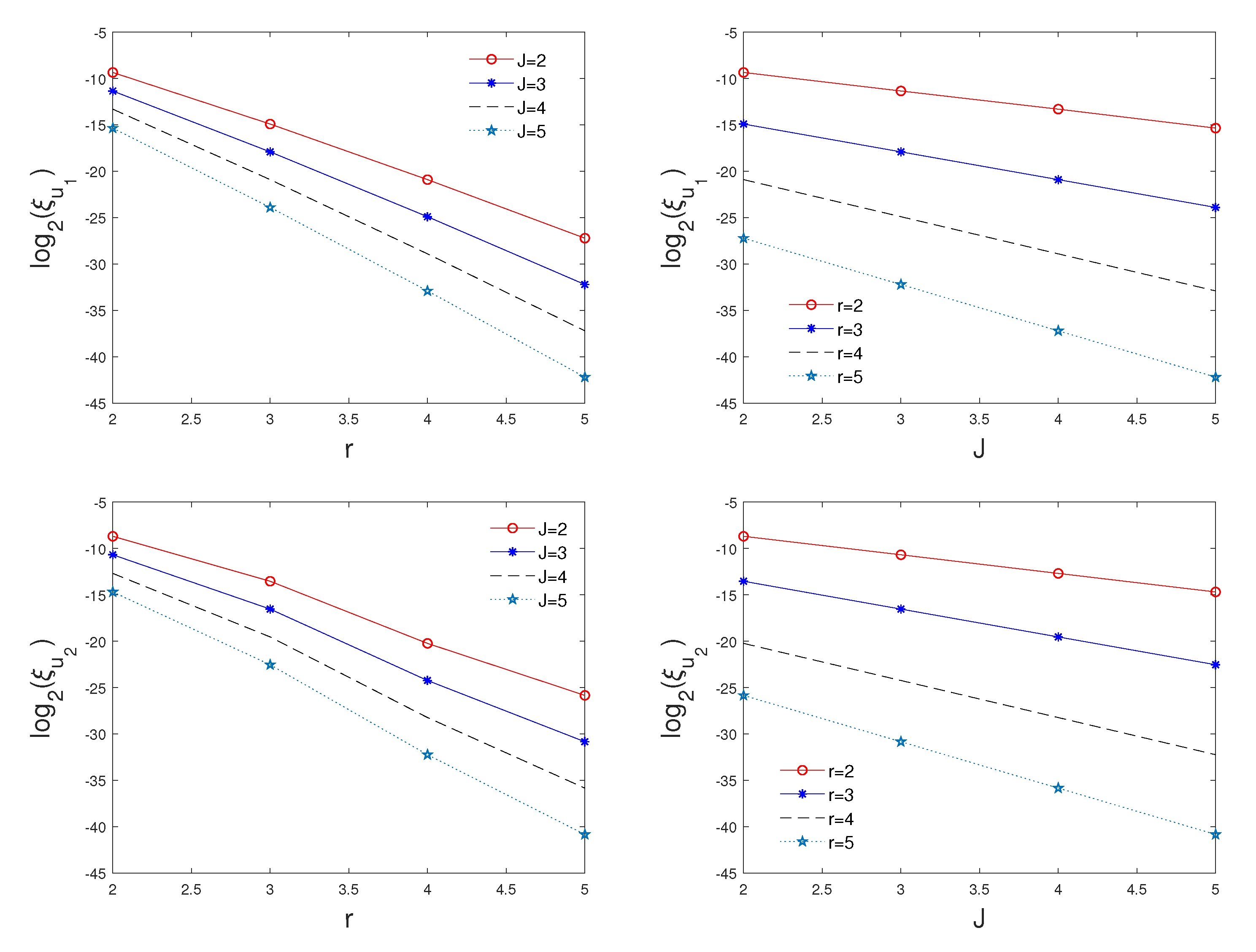
Figure 1.
Effects of the refinement level J (left) and the multiplicity parameter r (right) on error when and for Example 1.
Figure 1.
Effects of the refinement level J (left) and the multiplicity parameter r (right) on error when and for Example 1.

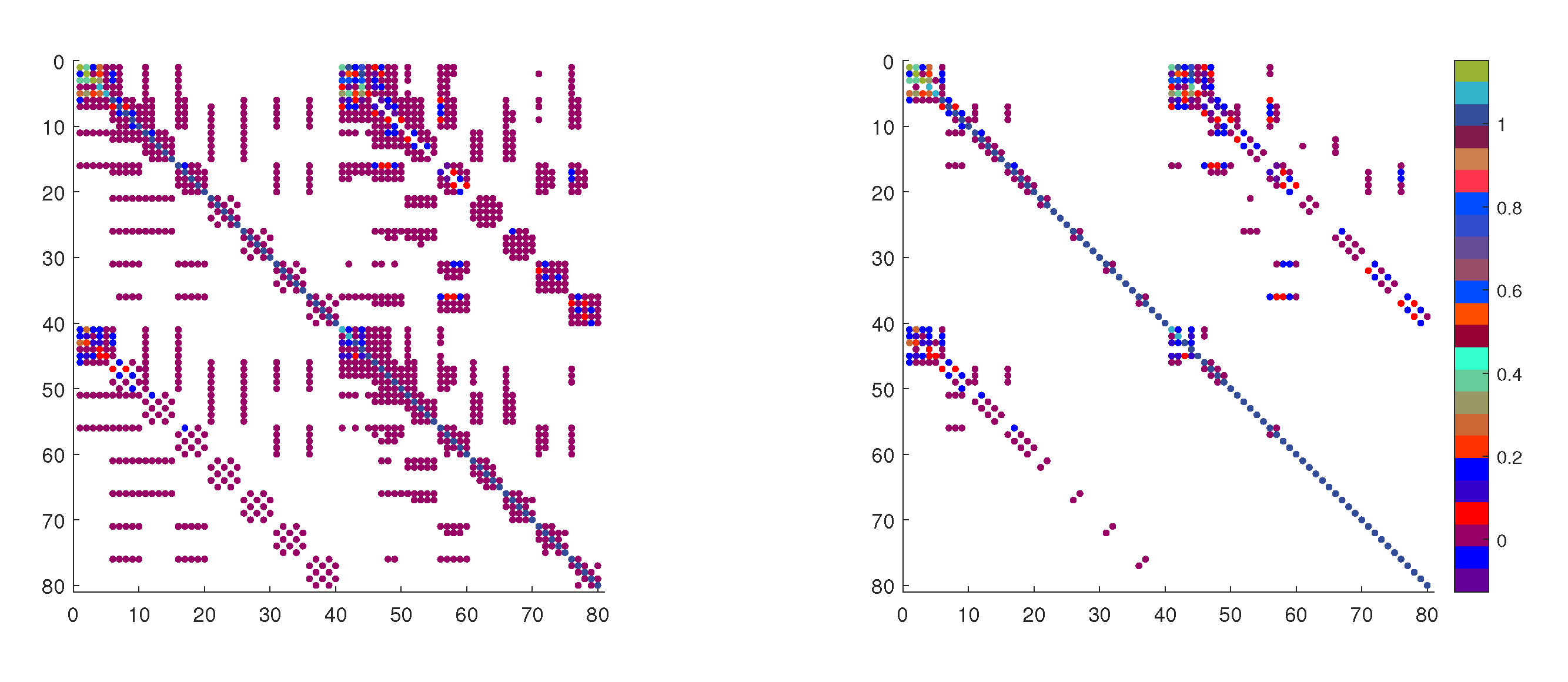
Figure 2.
Plot of sparse matrix after thresholding with (left) and (right) for Example 1.

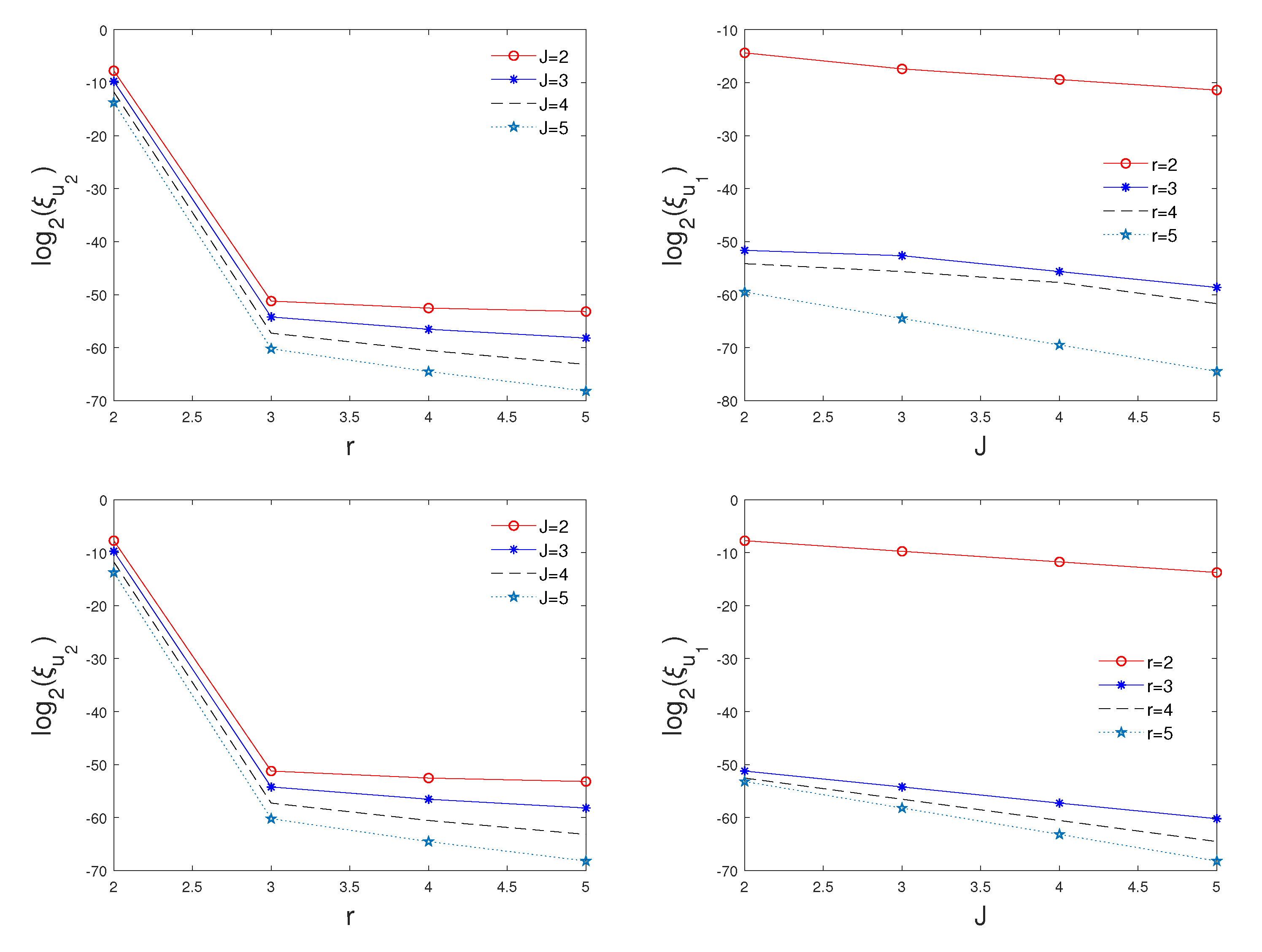
Figure 3.
Effects of the refinement level J (left) and the multiplicity parameter r (right) on error when and for Example 2.
Figure 3.
Effects of the refinement level J (left) and the multiplicity parameter r (right) on error when and for Example 2.

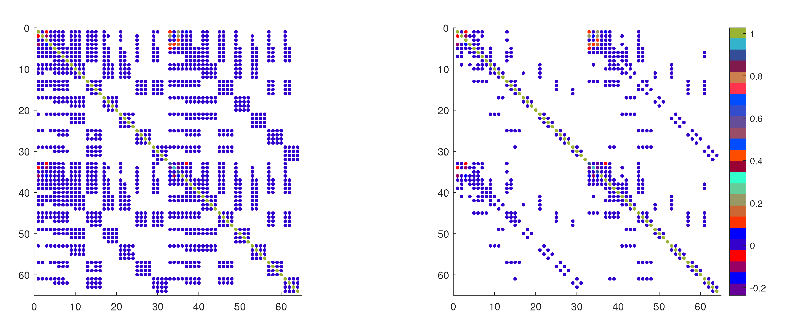
Figure 4.
Plot of sparse matrix after thresholding with (left) and (right) for Example 2.

Figure 5.
Plot of the exact and numerical solution taking and for Example 3.


Table 1.
Effects of parameters r, J and on sparsity and -error for Example 1.
| Without Thresholding | |||||||
|---|---|---|---|---|---|---|---|
| -Error | -Error | -Error | |||||
| 3 | 2 | 6.25 | |||||
| 3 | |||||||
| 5 | 2 | ||||||
| 3 | |||||||
Table 2.
Effect of the refinement level J and multiplicity parameter r on -error for Example 3.
| r | |||||
|---|---|---|---|---|---|
| 3 | |||||
| 4 | |||||
| 5 | |||||
| 3 | |||||
| 4 | |||||
| 5 |
© 2020 by the authors. Licensee MDPI, Basel, Switzerland. This article is an open access article distributed under the terms and conditions of the Creative Commons Attribution (CC BY) license (http://creativecommons.org/licenses/by/4.0/).
Share and Cite
MDPI and ACS Style
Long, H.V.; Jebreen, H.B.; Tomasiello, S. Multi-Wavelets Galerkin Method for Solving the System of Volterra Integral Equations. Mathematics 2020, 8, 1369. https://0-doi-org.brum.beds.ac.uk/10.3390/math8081369
AMA Style
Long HV, Jebreen HB, Tomasiello S. Multi-Wavelets Galerkin Method for Solving the System of Volterra Integral Equations. Mathematics. 2020; 8(8):1369. https://0-doi-org.brum.beds.ac.uk/10.3390/math8081369
Chicago/Turabian StyleLong, Hoang Viet, Haifa Bin Jebreen, and Stefania Tomasiello. 2020. "Multi-Wavelets Galerkin Method for Solving the System of Volterra Integral Equations" Mathematics 8, no. 8: 1369. https://0-doi-org.brum.beds.ac.uk/10.3390/math8081369
Note that from the first issue of 2016, this journal uses article numbers instead of page numbers. See further details here.