Insurance Contracts for Hedging Wind Power Uncertainty


1
Department of Economics, “G. D’Annunzio” University of Chieti-Pescara, 66013 CHIETI, Italy
2
Department of Economic and Business Science, “Guglielmo Marconi” University of Rome, 00185 Rome, Italy
3
Department of Management, Marche Polytechnic University, 60121 Ancona, Italy
*
Author to whom correspondence should be addressed.
Mathematics 2020, 8(8), 1376; https://0-doi-org.brum.beds.ac.uk/10.3390/math8081376
Submission received: 30 July 2020
/
Revised: 12 August 2020
/
Accepted: 14 August 2020
/
Published: 17 August 2020
(This article belongs to the Special Issue New Trends in Random Evolutions and Their Applications)
Abstract
:This paper presents an insurance contract that the supplier of wind power may subscribe to with an insurance company in order to immunize his/her revenue against the volatility of wind power and prices. Based on empirical evidence, we found that wind power and electricity prices are correlated. Then, we adopted a joint stochastic process to model both time series, which is based on indexed semi-Markov chains for the wind power generation process and on a general Markovian process for the electricity price process. Using a joint stochastic model allows the insurance company to compute the fair premium that the wind power producer has to pay in order to hedge the risk against inadequate revenues. Recursive type equations are obtained for the prospective mathematical reserves of the insurance contract. The model and the validity of the results are illustrated through a real data application.
1. Introduction
The use of renewable energies is continuously expanding year-by-year, and this trend is expected to persist in the future, although a decline of capacity has been observed related to lockdown measures due to the COVID-19 outbreak during 2020; see [1].
Wind energy covers a large part of renewable energy production even if this industry suffers the high variability of the wind speed process, which in turn impacts the electricity generation.
To remedy this problem, several solutions have been considered. Some of them are of a technical nature; others are based on intangible instruments such as financial products and specific contracts. Among the technical solutions, we remember the recourse to energy storage systems based on batteries that can contribute to absorbing the excess of production during high wind speed periods and to yield required power during low wind speed moments. The literature on this aspect is very large, and we may refer to [2,3,4,5,6] and to the respective bibliographies. Another technical possibility is associated with hybrid power plants that help wind power production with any dispatchable energy source such as gas turbines, air compressed systems, hydroelectric plants, or different; see, e.g., [7]. These engineering-based approaches need sophisticated technical know-how that may be outside of the wind power producer’s possibilities. For this reason, alternative solutions based on intangible instruments have been proposed and revealed to be practicable. Some of them are based on the possibility for the wind farm to purchase call/put options to protect itself against the uncertainty of the wind; see [8,9] on devising a barrier option for wind power. A more recent proposal came from [10] where an insurance contract was advanced as an effective tool to hedge wind speed volatility and in turn wind power. The main idea of the insurance-driven approach is to design an insurance contract that may protect the wind power producer (WPP) from undesirable fluctuation of the income generated by the wind power production. The contract is based on an exchange of cash-flows in terms of premium paid and benefits obtained by the WPP that should respect a form of equilibrium. Premiums are paid periodically and are for simplicity constant in time. Benefits are collected in case the wind power sold at the market price of electricity is unable to generate the desired income stipulated in the contract. Accordingly, the paramount objective of this paper is to compute the level of fair premium and the evolution of the mathematical reserves generated by the cash-flows. This approach requires the specification of an accurate wind power model. In [10], the authors applied a weighted indexed semi-Markov chain model (WISMC), which has been proven to possess a suitable probabilistic structure able to reproduce many stylized facts of wind speed and power dynamics; see [11,12,13,14]. This class of stochastic processes is a generalization of semi-Markov processes, which have shown to be very appropriate in a wide spectrum of domains ranging from reliability to finance; see, e.g., [15,16,17].
Nevertheless, the contribution by [10] leaves open space for further improvements. First, it is well known that electricity price evolves randomly in time; see, e.g., [18,19]. Thus, the unrealistic assumption of the deterministic electricity price adopted in [10] should be relaxed in favor of stochastic process assignment. Second, we also know that the electricity price is correlated with the wind power production process because large wind power productions are associated with decreases in the electricity price as an excess of supply on the market; see, e.g., [7,20]. This empirical evidence suggests the adoption of the multivariate model of the wind power generation and electricity price process. For this reason, we propose a multivariate model of wind the energy production and electricity price process using copula functions. After having specified the model, we describe the actuarial structure of the insurance contract, and we derive a recurrent type equation for the expected value of the accumulated discounted benefit function over a given time interval. Consequently, we determine the fair premium and an equation for the prospective mathematical reserve. The model is applied to real data concerning the electricity price process and wind production in Sardinia from 1 August 2014 to 31 July 2018. We show how to fix the fair premium and the computation of the connected actuarial quantities.
From a mathematical point of view, it is relevant to observe that the considered mathematical methods presented in this paper are generalizations of methods proposed in other classical problems of insurance mathematics like life insurance contracts and disability modeling where multi-state models based on Markov chains (see, e.g., [21,22,23]) or semi-Markov chains (see, e.g., [24,25,26,27,28,29,30,31,32,33]) with rewards represent the usual approach. The rest of the paper is organized as follows. In Section 2, we briefly describe the WISMC model of wind energy and the joint model of electricity price and wind power generation. This fixes the framework in which the actuarial evaluation will be subsequently developed. We then present in Section 3 the actuarial investigation with the description of the insurance contract, the computation of the fair premium, and the evolution of the mathematical reserve. In Section 4, we present a numerical example based on real data on wind power production and electricity prices.
2. The Stochastic Models
In this section, we describe the main stochastic tools adopted for the description of the considered insurance contract. We first present the WISMC model that is used as a marginal model for wind power production. Successively, we introduce a Markovian model for the electricity price process, and using a copula function, we specify a dependence structure between electricity price and wind power production. In this way, we obtain a multivariate model that is at the base of the valuation of the insurance contract.
2.1. The WISMC Model of Wind Power Production
Here, we introduce the discrete-time WISMC model with a finite state space in relation to the wind power production of a wind farm.
Indexed semi-Markov models are based on three sequences of random variables defined on a common complete probability space . First, we consider the stochastic process with values in . The set E denotes different levels of wind power production. These levels change value in time due to randomness inherent to the wind power production phenomenon, and describes the sequences of wind power transitions from one level to another one in time.
Evidently, the wind power production stays at a given level of production for a random time before changing its value. Accordingly, there is another sequence of random variables denoted by that indicates the times when the change of states of occurs. The sequence is an increasing sequence of random times, and their difference is called the sequence of sojourn times. Thus, the random variable denotes how long the wind power state will remain at level before making a transition to level .
A detailed description of the system needs the specification of the so-called index process that we are going to introduce.
Assume disposing of a set of past information about wind power levels and transition times, i.e.,
then consider a generic bounded function called the score function, and define the index process as:
A specific choice of the score function may depend on the considered application and will be discussed later in the applied section. The quantity is the memory parameter and is used to calibrate the overall memory of the process to the real data. Different values of could be used according to the need to make more relevant the information brought by the past observations. The calibration of will also be discussed later in the application. From an intuitive point of view, the index process assigns to a past trajectory of wind power production a total score. This is done by attaching to every past wind power observation a score , which depends on the recorded value of the wind power , on when this observation was registered, and on the present time .
These three random processes are assumed to interact, and therefore, we specify a dependence structure between them. Specifically, we assume that:
where is the natural filtration of the three-variate process.
Relation (2) asserts that the knowledge of the last wind power value and of the value of the index process suffices to give the conditional distribution of the couple , whatever the values of the past variables might be. This means that knowing the couple , we dispose of the joint distribution of the next wind power value and of the time when the system will enter into . This model is particularly able to increase the memory of the process incorporating past information about the system’s evolution. It should be remarked that whenever should be constant with respect to v for all possible combinations of , then the WISMC model collapses into a standard semi-Markov chain model.
Let be the sojourn time cumulative distribution function in wind power state with index process value v, that is:
It expresses the probability to change the actual wind power i in a time less than or equal to t given the indexed process has value v. The standard notation for the survival function is adopted hereafter, i.e., .
Let be the number of transitions held up to time t, and let be the state of the system (wind power) at time t. We refer to as a weighted-indexed semi-Markov chain and to as the indexed embedded Markov chain.
The processes provide a description of the status of the system when a transition occurs, i.e., in correspondence to any one of the jump times . However, during any time t belonging to a sojourn time (that is for ), while the state of the wind power remains unchanged (), the value of the index process updates due to the information that the embedded Markov chain has not changed state along the sojourn time or, equivalently, the time elapsed since the last transition has increased. The time elapsed since the last transition is called the backward recurrence time process and is defined by . Thus, to completely characterize the status of the system also along a sojourn time, it is necessary to extend the definition of the index process allowing considering any time as follows:
where . It is not difficult to realize that if , then , and accordingly:
Now, observing that the previous relations imply that , by substitution in (4), we get:
which coincides with (1) and shows that .
Let us introduce the marginal one-step distribution of WISMC:
In our application, it denotes the conditional probability distribution of wind power production at time given the values of the wind power production and the backward and index processes at time t.
This probability can be obtained as follows:
where
The probabilities can be obtained from the knowledge of the kernel of the WISMC according to Lemma 2.1 and Theorem 2.1 in [34]. We conclude this short overview on the WISMC model by considering two concepts that we need to introduce. They are taken from [35] and play an important role in the determination of the results of this study.
Definition 1.
[Shift operator] Let be a sequence of states and corresponding transition times, i.e., , , .
Denote , then we define the shift operator:
defined by:
where , , .
Intuitively, the shift operator when it is applied to a trajectory renders back another trajectory where the sequence of visited states is the same as in the input trajectory with the difference that transition times are translated to time units backward and the number of transitions is set one unit backward.
The following assumption concerning the score function will be needed in the rest of the article:
Assumption 1.
, .
Lemma 1.
For a WISMC with score function that satisfies Assumption 1, for fixed arbitrary state j and time t and , we have:
The result presented in Lemma 1 focuses on a class of score functions leading the probability (7) to be independent of n. Accordingly, the WISMC inherits a homogeneity property that is particularly useful for the applications of the model. Throughout this article, we are going to consider only homogeneous WISMC.
2.2. Joint Model of Electricity Price and Wind Power Production
A wind power producer (WPP) sells energy in the spot market. Accordingly, he/she will accept the market price of electricity as a counterpart for his/her power production. The electricity price changes in time randomly, and different stochastic processes have been advanced as a suitable description of the statistical properties of this variable. A very exhaustive review and perspective were given in [18].
In this paper, we focus on a simple structure for the electricity price model that can be merged, successively, with the WISMC model of wind power production. For this reason, we focus on a stochastic process that satisfies a general Markovian property. Precisely, we assume:
Assumption 2.
The energy price dynamics satisfies the Markov property, i.e.,
A large variety of models satisfies this property, and an example is given by:
where is a Gaussian noise. Equation (8) defines a first-order autoregressive model (AR(1)) that exhibits a mean reversion property. Extensions to AR(p) models fall well within our framework, as well as processes that allow the presence of a jump component:
where is a pure jump process.
The observation of data on electricity prices and wind power production suggests the presence of a dependence structure between these random processes; see, e.g., [7,20]. In general, it is expected that if a large amount of wind power is introduced into a power system, this would tend to lower the spot price on the related energy market. Motivated by this empirical evidence, we advance another assumption:
Assumption 3.
The wind power production and the electricity price are dependent processes. Their joint probability distribution satisfies the following property:
where is the sigma algebra generated by the WISMC (which includes information on past values of the backward recurrence time process and of the index process as well). The symbol is used to denote a copula function, which merges the conditional marginal distribution of electricity price:
and the conditional marginal one-step distribution of wind power production:
Thus, once the marginal models of electricity price and wind power are settled on, the adoption of a specific copula function leads to a joint model that is at the base of the actuarial problem we are going to discuss in the next section.
3. The Insurance Problem
In this section, we argue that a WPP may protect himself/herself against the variability of the income generated through its activity using actuarial techniques. Let be the WPP’s revenues collected at time t by producing a level of wind power that is sold on the market at the price . The process is complex and is subject to consistent variability in time due to its basic components: the produced wind power , the electricity price process , and their dependence structure.
Here, we consider the possibility to hedge this risk using an insurance contract.
At any time , the WPP collects random revenues . Assume, he/she wishes to guarantee for himself/herself at any time s at least a revenue equal to . To this end, he/she may sign an insurance contract such that:
- if , he/she gets from the insurer the benefit ;
- if , no money transfer from the insurer to the WPP occurs;
- at any time during the validity period of the contract, he/she pays a fixed premium to the insurer equal to .
- money amounts are discounted with fixed discount factor v; accordingly, denotes the discount factor for s periods of time.
A traditional problem in actuarial mathematics is how to determine the value of the premium U. The simplest way is to fix U in such a way that premiums and benefits are in equilibrium over a considered time interval. Thus, let be the total benefits paid by the insurer during the time interval :
The dependence on three time variables is considered with the intention of considering explicitly the effects of the last transition time (), the time u elapsed in the last state until current time (), and the horizon time of evaluation T.
Clearly, is a random process that inherits statistical properties from the revenue process . A viable solution is to define the total fair premium as the amount such that is equal to the expected value of the benefits, i.e., .
The fair premium can now be determined as the amount U such that:
where represents the present value of an annuity due, which is a series of unit payments at the beginning of each period for periods discounted using the interest rate . Thus, the possibility to determine the fair premium passes from the computation of the total expected benefits . To this end, denote by the random variable that has the same distribution as the conditional distribution of the random variable given that:
Finally, denote by:
the conditional expectation with respect to the information available up to present time , which includes past values of the wind power production, corresponding transition times, backward recurrence time process value, and electricity price.
Lemma 2.
Under Assumptions 1–3, the accumulated discounted benefit process satisfies the following stochastic relation:
and consequently:
Proof.
To show that:
and:
share the same distribution, it is sufficient to remark that these random variables are obtained by the summation of the same addends, which are discounted by the same time length. These random addends have the same conditional distribution even if they are defined on different information sets, which are:
for (14) and:
for (15). Nonetheless, from Assumption A2, we have that:
having denoted by the distribution of X. Moreover, from Lemma 1 in [35], we can obtain that, given , the index process assumes the value:
and the same value is assumed conditional on , i.e., . This implies that:
The first-order moment of the accumulated discounted benefits can now be calculated using the relation derived in the next theorem.
Theorem 1.
Under Assumptions 1–3, the expected value of accumulated discounted benefits satisfies the following recurrent equations, for all , , and ,
where , and:
Proof.
Since , we have that:
Let be the indicator variable for event E, then the expectation (20) can be further decomposed into:
Formula (21) can be obtained according to the integral representation of expectation as follows:
Observe now that the event implies that , and consequently, the former integral becomes
The conditional joint distribution of the random vector inside Formula (23) can be derived using Assumption 3 as a function of the copula and the marginal distributions of wind power production and electricity price process. Indeed, for small , we have:
where:
and:
Firstly, it is worth observing that this joint distribution is of a mixed type, having a continuous part () and a discrete one (). Secondly, the expression (uid38) is in agreement with a general formula for multivariate mixed distributions presented in [36].
The relation:
is therefore valid.
To compute the expectation in Formula (21), we observe that the event implies that . We use then the integral representation of expectation and analogous computations as we did before to get:
It remains to compute Formula (20). It is simple to realize that:
The latter expression can be rewritten using the tower property of conditional expectation as follows:
Observe that the random variable:
is distributed the same as:
By integration, we obtain:
Similarly, one obtains for the second part of (31) that:
which completes the proof of the theorem. □
Remark 1.
Theorem 1 can be seen as an extension of Theorem 1 in [29] and also of those obtained in [10] to the more general framework represented by WISMC models. More precisely, our result includes the possibility to manage random rewards that are not only a deterministic function of the state of the chain, but that are obtained through a transformation of a stochastic process (electricity price process), which is dependent through a copula function on the state process (wind power production) modeled using a WISMC model.
Theorem 1 determines an expression for the expected value of paid benefits during the validity period of the contract. Therefore, if the premium is fixed according to Relation (10), at any time s, we have the generation of a payment (positive or negative) equal to:
which guarantees a global balance during the time interval . Anyway, the accumulation process of premiums and benefits is not in equilibrium at any time where an excess of paid premiums or received benefits may occur. To quantify this payment process, which is important to understand the cash-flows associated with the contract, it is sufficient to replace the time T (maturity of the insurance contract) in Equation (19) by time L and to consider payments according to Relation (32). To this end, if we denote by the accumulated rewards from the inception time up to the time L and by the random variable, which has the same distribution as the conditional distribution for the r.v. given that the past information is , , , we can set and obtain a recursive equation for the so-called prospective reserve , i.e.,
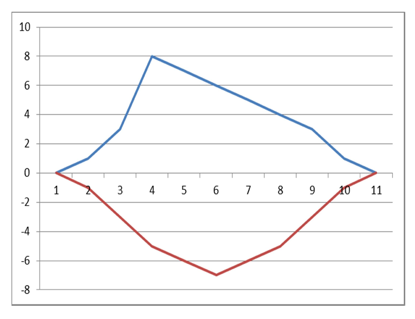
The quantity expresses the average level of payments up to time L. A positive value of denotes the fact that up to time L, there was an excess of benefits with respect to premiums. Conversely, a negative value of indicates that premiums were paid in excess as compared to the benefits. Obviously, at the maturity, T of the contract premiums and benefits should be in equilibrium; therefore, .
The knowledge of the prospective reserve is very important in insurance mathematics because a positive function highlights the need to charge the fair premium in such a way to avoid that on average, the insurance company will pay in advance. This prevents the contract from not being self-financed.
As a matter of example, we show in Figure 1 two hypothetical paths of the prospective reserve. Both curves start from zero and at the end of the contract assume a null value. The positive curve denotes a contract not self-financed, needing the introduction of a charge over the fair premium due to expected benefits, which forgo expected premiums. The negative curve indicates a contract that is self-financed due to expected premiums forgoing expected benefits.
4. Materials and Methods
The data covered a 4 year period (from 1 August 2014 to 31 July 2018) on an hourly basis. The wind speed dataset was retrieved from the modern-era retrospective analysis for research and applications, version 2 (MERRA-2) project (https://gmao.gsfc.nasa.gov/reanalysis/MERRA-2/).
The data concerning electricity price are freely available from the website of the Italian company “Gestore Mercati Energetici” at (http://www.mercatoelettrico.org/It/download/DatiStorici.aspx). We obtained the data for the Sardinia zone, covering the period described before on an hourly basis.
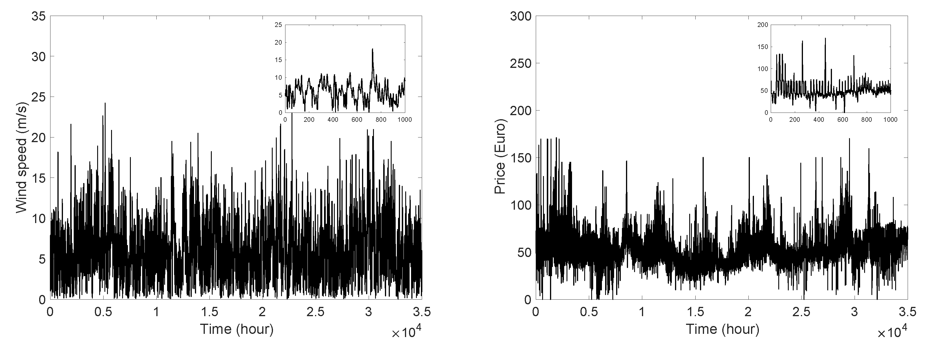
The time series of wind speed and prices for the analyzed period are shown in Figure 2.
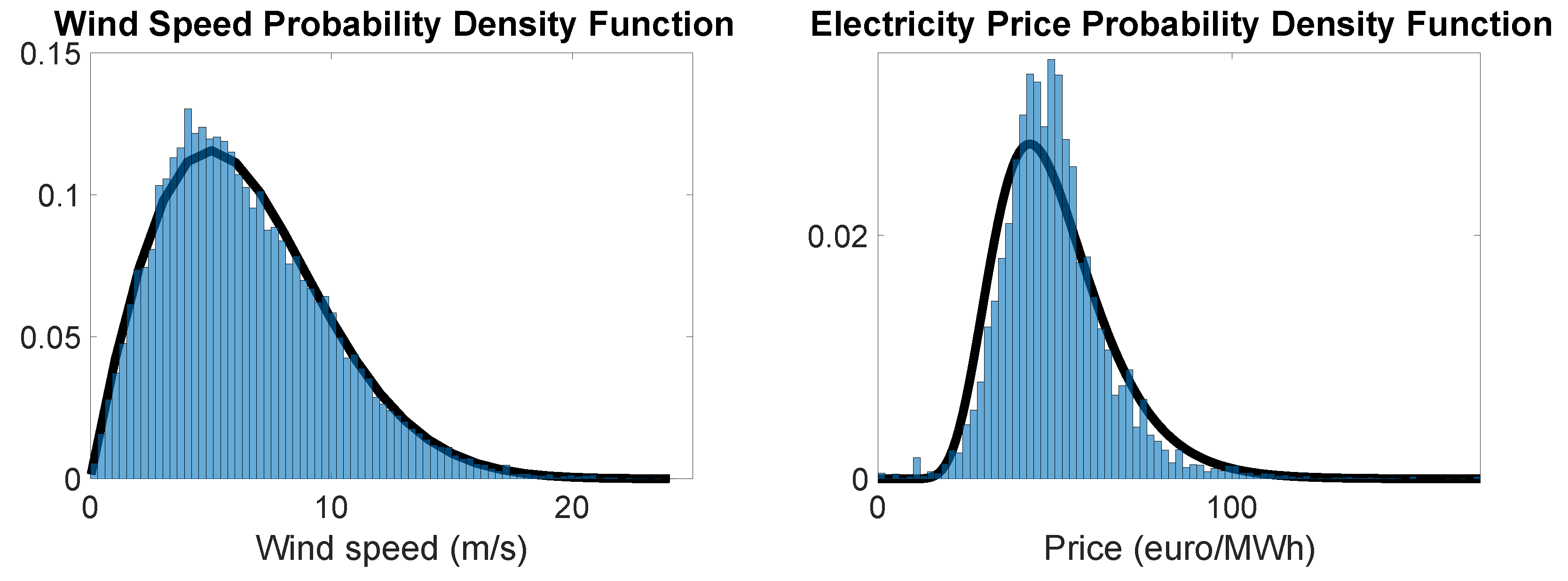
We also plotted the empirical probability density function of both variables (Figure 3) and compared them with a Weibull distribution for wind speed and a lognormal distribution for prices
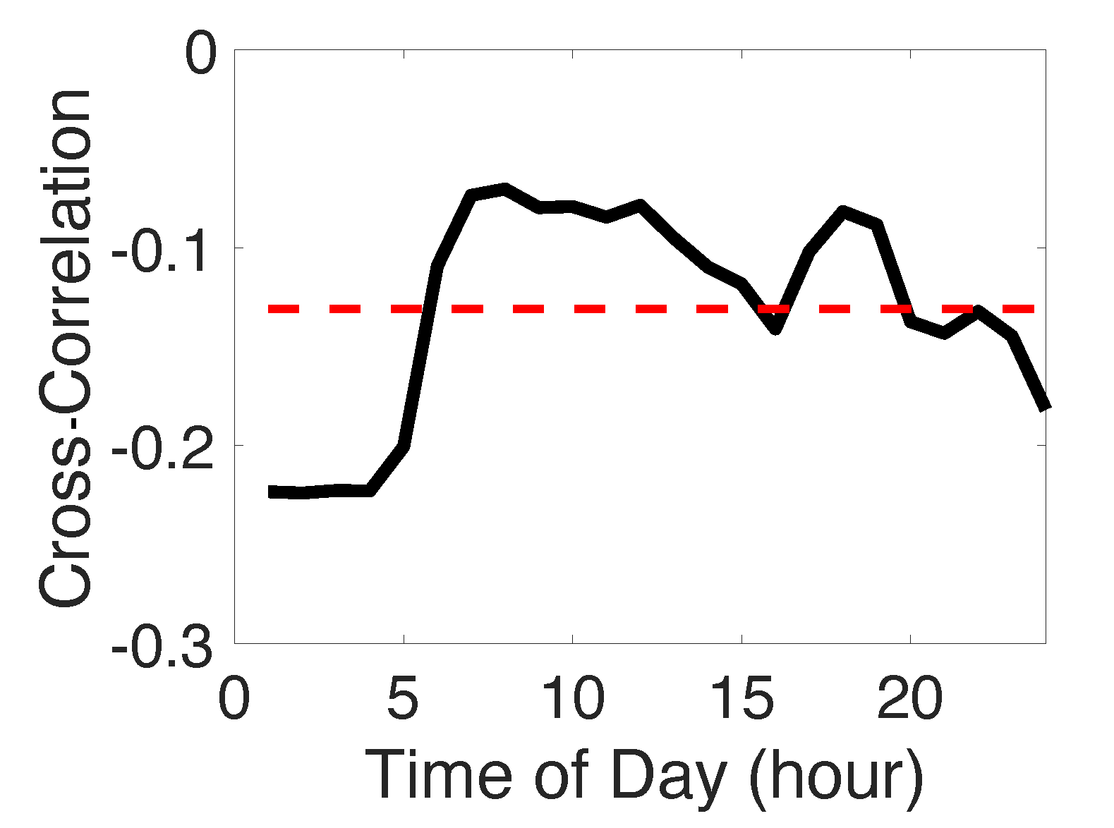
We also deduced a dependence between price and wind speed that gave rise to low negative correlation that had a small variation during the day; see Figure 4. As a consequence, this correlation should be carefully managed.
To obtain the energy produced by one wind turbine, we transformed the wind speed in wind power by means of the power curve of a hypothetical wind turbine. The turbine is located in Sardinia (Italy) and has the following characteristics:
- -
- geographical coordinates: 39.5 N (latitude) and 8.75 E (longitude);
- -
- hub height of the turbine: 95 m;
- -
- rated power of the turbine: 2 MW;
- -
- cut-in wind speed: 4 m/s;
- -
- rated wind speed: 13 m/s;
- -
- cut-out wind speed: 25 m/s.
To extend the analysis to a wind farm that consists of multiple turbines, as a first approximation, it is possible to multiply the wind energy produced by the number of turbines.
According to Section 2.1, wind power was modeled by using a WISMC model. The parameters were optimized by using the algorithms described in [10,37]. Following the same works, we chose an exponentially weighted moving average (EWMA) of the past wind speed values to define the index process.
Then, wind power was discretized into nine states with the cited optimization algorithm that reduced the mean squared error between the real power autocorrelation function and the simulated one. According to [20], we selected the process for the electricity price time series. Then, we modeled correlation between prices and wind power production by using a Gaussian copula. All parameters, for price time series and the copula, were optimized by using the MLE algorithm implemented in MATLAB software. To compare our model with real data, we generated synthetic trajectories of the joint process of wind power and electricity prices of the same time length of the real database by means of Monte Carlo simulations.
5. Results on the Insurance Problem
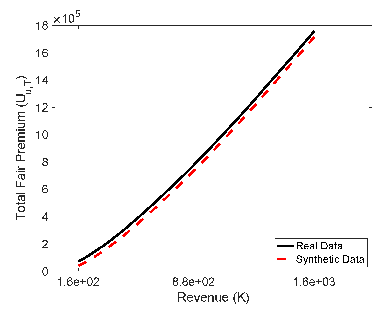
In Figure 5, we compare the fair premium as defined in Equation (10) for real data and simulated data as a function of the revenue K. We used the hypothesis that the premium and benefits are settled daily. All values were actualized by using a constant interest rate fixed at (the use of a term structure for the interest rate can be implemented easily). In the plot, the dashed line represents simulated data, while the continuous line represents real data. It is obvious from the figure that the model is able to reproduce perfectly the real behavior. As expected, the fair premium is an increasing function of the revenue K.
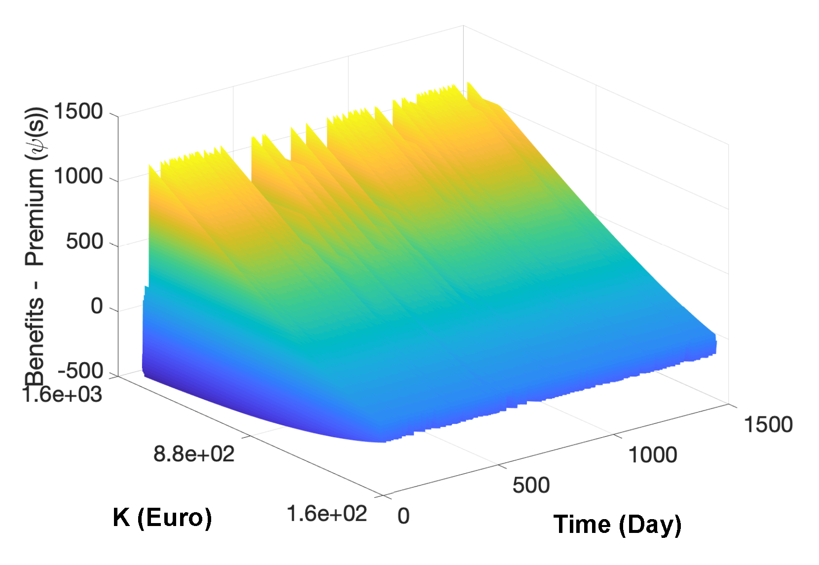
In Figure 6 the daily difference between benefits and the periodic premium is calculated as a function of time and revenue K. As one would expect, this difference is a random variable, and the variance increases with the revenue value.
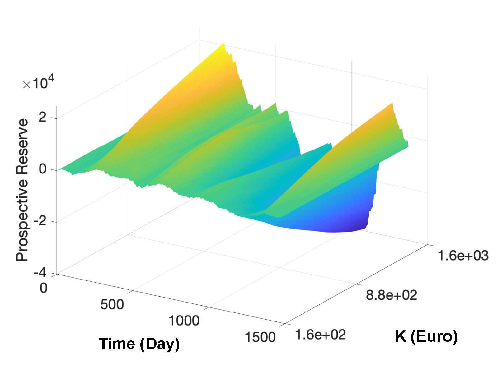
As the last result, in Figure 7, we show the prospective reserve, again as a function of time and revenue. According to the theoretical results, the reserve starts from zero and reaches a zero value at the end of the contract. Like the difference between benefits and premium, the prospective reserves deviate from zeros more for increasing values of the revenue K.
6. Conclusions
In this paper, we showed how to model jointly wind power and electricity prices that, according to real data, have a small negative correlation, which, nonetheless, cannot be ignored. The advanced joint stochastic process is based on indexed semi-Markov chains for the wind power generation process and on a general Markovian process for the electricity price process, which are merged through copula functions. The joint process is used to compute the fair premium and the prospective mathematical reserve for an insurance contract that a wind power producer can stipulate to hedge himself/herself from the risk of low revenues. The results are a generalization to a dependent framework of results obtained in the case of constant electricity prices, which are independent of the power process by [10]. We presented the computation of the most relevant insurance quantities both from a mathematical and an empirical point of view. The empirical results show a very good agreement between real and synthetic data obtained from Monte Carlo simulations. Nevertheless, this mathematical approach suffers from a few limitations. The first is due to its probabilistic structure, which can only be applied in the presence of a consistent dataset with many observations. For example, the same application could not be executed on data sampled on monthly or even weekly time scales. The second limitation concerns the choice of the score function that defines the index process, which is not yet automatized and only done in a heuristic way. Further developments of the model including the computation of the retrospective mathematical reserve and the adoption of more general schemes for computing the premium that go beyond the application of the fair premium principle seem highly promising. Although such considerations on wind insurance are entirely theoretical at the moment, they may have interesting practical implications and allow insurance companies to enter into a new business line.
Author Contributions
All authors contributed equally to this work. All authors read and agreed to the published version of the manuscript.
Funding
This research received no external funding.
Conflicts of Interest
The authors declare no conflict of interest.
References
- IEA. Renewable Energy Market Update. 2020. Available online: https://www.iea.org/reports/renewable-energy-market-update (accessed on 15 May 2020).
- Beenstock, M. The stochastic economics of windpower. Energy Econ. 1995, 17, 27–37. [Google Scholar] [CrossRef]
- Barton, J.P.; Infield, D.G. Energy storage and its use with intermittent renewable energy. IEEE Trans. Energy Convers. 2004, 19, 441–448. [Google Scholar] [CrossRef]
- Sufyan, M.; Rahim, N.A.; Aman, M.M.; Tan, C.K.; Raihan, S.R.S. Sizing and applications of battery energy storage technologies in smart grid system: A review. J. Renew. Sustain. Energy 2019, 11, 014105. [Google Scholar] [CrossRef]
- Wang, X.; Vilathgamuwa, D.M.; Choi, S.S. Determination of battery storage capacity in energy buffer for wind farm. IEEE Trans. Energy Convers. 2008, 23, 868–878. [Google Scholar] [CrossRef]
- Pinson, P.; Papaefthymiou, G.; Klockl, B.; Verboomen, J. Dynamic sizing of energy storage for hedging wind power forecast uncertainty. In Proceedings of the 2009 IEEE Power & Energy Society General Meeting, Calgary, AB, Canada, 26–30 July 2009; pp. 1–8. [Google Scholar]
- D’Amico, G.; Petroni, F.; Sobolewski, R.A. Optimal Control of a Dispatchable Energy Source for Wind Energy Management. Stochastics Qual. Control 2019, 34, 19–34. [Google Scholar] [CrossRef]
- Hedman, K.W.; Sheblé, G.B. Comparing hedging methods for wind power: Using pumped storage hydro units vs. options purchasing. In Proceedings of the 2006 International Conference on Probabilistic Methods Applied to Power Systems, Stockholm, Sweden, 11–15 June 2006; pp. 1–6. [Google Scholar]
- Xiao, Y.; Wang, X.; Wang, X.; Wu, Z. Trading wind power with barrier option. Appl. Energy 2016, 182, 232–242. [Google Scholar] [CrossRef]
- D’Amico, G.; Petroni, F.; Prattico, F. Insuring wind energy production. Phys. A Stat. Mech. Appl. 2017, 467, 542–553. [Google Scholar] [CrossRef]
- D’Amico, G.; Petroni, F.; Prattico, F. Wind speed modeled as an indexed semi-Markov process. Environmetrics 2013, 24, 367–376. [Google Scholar] [CrossRef] [Green Version]
- D’Amico, G.; Petroni, F.; Prattico, F. Wind speed and energy forecasting at different time scales: A nonparametric approach. Phys. A Stat. Mech. Appl. 2014, 406, 59–66. [Google Scholar] [CrossRef] [Green Version]
- D’Amico, G.; Petroni, F.; Prattico, F. Economic performance indicators of wind energy based on wind speed stochastic modeling. Appl. Energy 2015, 154, 290–297. [Google Scholar] [CrossRef]
- D’Amico, G.; Petroni, F.; Prattico, F. Reliability measures for indexed semi-Markov chains applied to wind energy production. Reliab. Eng. Syst. Saf. 2015, 144, 170–177. [Google Scholar] [CrossRef] [Green Version]
- Limnios, N.; Oprisan, G. Semi-Markov Process and Reliability. 2001. Available online: file:///C:/Users/MDPI/Downloads/bok3A978-1-4612-0161-8.pdf (accessed on 15 May 2020).
- Barbu, V.S.; Limnios, N. Semi-Markov Chains and Hidden Semi-Markov Models toward Applications: Their Use in Reliability and DNA Analysis; Springer Science & Business Media: Berlin/Heidelberg, Germany, 2009; Volume 191. [Google Scholar]
- Swishchuk, A.; Hofmeister, T.; Cera, K.; Schmidt, J. General semi-Markov model for limit order books. Int. J. Theor. Appl. Financ. 2017, 20, 1750019. [Google Scholar] [CrossRef]
- Weron, R. Electricity price forecasting: A review of the state-of-the-art with a look into the future. Int. J. Forecast. 2014, 30, 1030–1081. [Google Scholar] [CrossRef] [Green Version]
- Mari, C. Hedging electricity price volatility using nuclear power. Appl. Energy 2014, 113, 615–621. [Google Scholar] [CrossRef]
- Casula, L.; D’Amico, G.; Masala, G.; Petroni, F. Performance estimation of a wind farm with a dependence structure between electricity price and wind speed. World Econ. 2020. [Google Scholar] [CrossRef]
- Norberg, R. A Time-Continuous Markov Chain Interest Model with Applications to Insurance. Appl. Stoch. Model. Data Anal. 1995, 11, 245–256. [Google Scholar] [CrossRef]
- Milbrodt, H. Hattendorff’s theorem for non-smooth continuous-time Markov models I: Theory. Insur. Math. Econ. 1999, 25, 181–195. [Google Scholar] [CrossRef]
- Henriksen, L.F.B.; Nielsen, J.W.; Steffensen, M.; Svensson, C. Markov chain modeling of policyholder behavior in life insurance and pension. Eur. Actuar. J. 2014, 4, 1–29. [Google Scholar] [CrossRef]
- Janssen, J. Application des processus semi-Markoviens à un probléme d’invalidité. Bulletin de l’Association Royale des Actuaries Belges 1966, 63, 35–52. [Google Scholar]
- Hoem, J.M. Inhomogeneous Semi-Markov Processes, Select Actuarial Tables, and Duration-dependence in Demography. In Population Dynamics; Elsevier: Amsterdam, The Netherlands, 1972; pp. 251–296. [Google Scholar]
- Janssen, J.; De Dominicis, R. Finite non-homogeneous semi-Markov processes: Theoretical and computational aspects. Insur. Math. Econ. 1984, 3, 157–165. [Google Scholar] [CrossRef]
- Janssen, J.; Manca, R. A realistic non-homogeneous stochastic pension fund model on scenario basis. Scand. Actuar. J. 1997, 1997, 113–137. [Google Scholar] [CrossRef]
- Stenberg, F.; Manca, R.; Silvestrov, D. Semi-Markov Reward Models for Disability Insurance. 2006. Available online: http://dspace.nbuv.gov.ua/bitstream/handle/123456789/4468/2006_12_3-4_17.pdf (accessed on 15 May 2020).
- Stenberg, F.; Manca, R.; Silvestrov, D. An algorithmic approach to discrete time non-homogeneous backward semi-Markov reward processes with an application to disability insurance. Methodol. Comput. Appl. Probab. 2007, 9, 497–519. [Google Scholar] [CrossRef]
- D’Amico, G.; Guillen, M.; Manca, R. Full backward non-homogeneous semi-Markov processes for disability insurance models: A Catalunya real data application. Insur. Math. Econ. 2009, 45, 173–179. [Google Scholar] [CrossRef]
- Ji, M.; Hardy, M.; Li, J.S.H. A semi-Markov multiple state model for reverse mortgage terminations. Ann. Actuar. Sci. 2012, 6, 235–257. [Google Scholar] [CrossRef]
- Maegebier, A. Valuation and risk assessment of disability insurance using a discrete time trivariate Markov renewal reward process. Insur. Math. Econ. 2013, 53, 802–811. [Google Scholar] [CrossRef]
- Buchardt, K.; Møller, T.; Schmidt, K.B. Cash flows and policyholder behaviour in the semi-Markov life insurance setup. Scand. Actuar. J. 2015, 2015, 660–688. [Google Scholar] [CrossRef]
- D’Amico, G.; Petroni, F. Multivariate high-frequency financial data via semi-Markov processes. Markov Process. Relat. Fields. 2014, 20, 415–434. [Google Scholar]
- D’Amico, G.; Petroni, F. A micro-to-macro approach to returns, volumes and waiting times. arXiv 2020, arXiv:2007.06262. [Google Scholar]
- Onken, A.; Panzeri, S. Mixed Vine Copulas as Joint Models of Spike Counts and Local Field Potentials. In Advances in Neural Information Processing Systems; Mit Press: Cambridge, MA, USA, 2016; pp. 1325–1333. [Google Scholar]
- D’Amico, G.; Petroni, F. Copula based multivariate semi-Markov models with applications in high-frequency finance. Eur. J. Oper. Res. 2018, 267, 765–777. [Google Scholar] [CrossRef]
Figure 1.
Two possible evolutions of the prospective mathematical reserve.

Figure 2.
Time series of wind speed and prices.

Figure 3.
Empirical pdf of wind speed fitted with a Weibull distribution and prices fitted with a lognormal distribution. The fits are performed by using an MLE algorithm.
Figure 3.
Empirical pdf of wind speed fitted with a Weibull distribution and prices fitted with a lognormal distribution. The fits are performed by using an MLE algorithm.

Figure 4.
Correlation between price and wind speed as a function of daily hours.

Figure 5.
Fair premium for real (continuous) and simulated (dashed) data as a function of the revenue K.
Figure 5.
Fair premium for real (continuous) and simulated (dashed) data as a function of the revenue K.

Figure 6.
Differences between benefits and the periodic premium as a function of time and revenue K.
Figure 6.
Differences between benefits and the periodic premium as a function of time and revenue K.

Figure 7.
Prospective reserve as function of time and revenue K.

© 2020 by the authors. Licensee MDPI, Basel, Switzerland. This article is an open access article distributed under the terms and conditions of the Creative Commons Attribution (CC BY) license (http://creativecommons.org/licenses/by/4.0/).
Share and Cite
MDPI and ACS Style
D’Amico, G.; Gismondi, F.; Petroni, F. Insurance Contracts for Hedging Wind Power Uncertainty. Mathematics 2020, 8, 1376. https://0-doi-org.brum.beds.ac.uk/10.3390/math8081376
AMA Style
D’Amico G, Gismondi F, Petroni F. Insurance Contracts for Hedging Wind Power Uncertainty. Mathematics. 2020; 8(8):1376. https://0-doi-org.brum.beds.ac.uk/10.3390/math8081376
Chicago/Turabian StyleD’Amico, Guglielmo, Fulvio Gismondi, and Filippo Petroni. 2020. "Insurance Contracts for Hedging Wind Power Uncertainty" Mathematics 8, no. 8: 1376. https://0-doi-org.brum.beds.ac.uk/10.3390/math8081376
Note that from the first issue of 2016, this journal uses article numbers instead of page numbers. See further details here.