A Comparison of Forecasting Mortality Models Using Resampling Methods


1
Departamento de Economía y Dirección de Empresas, Universidad de Alcalá, Pza. San Diego S/N, 28801 Alcalá de Henares, Spain
2
Centro de Gestión de la Calidad y del Cambio, Universitat Politècnica de València, Camino de Vera, S/N, 46022 Valencia, Spain
*
Author to whom correspondence should be addressed.
†
These authors contributed equally to this work.
Mathematics 2020, 8(9), 1550; https://0-doi-org.brum.beds.ac.uk/10.3390/math8091550
Submission received: 28 July 2020
/
Revised: 1 September 2020
/
Accepted: 7 September 2020
/
Published: 10 September 2020
(This article belongs to the Special Issue Application of Mathematical Analysis and Models to Financial Economics)
Abstract
:The accuracy of the predictions of age-specific probabilities of death is an essential objective for the insurance industry since it dramatically affects the proper valuation of their products. Currently, it is crucial to be able to accurately calculate the age-specific probabilities of death over time since insurance companies’ profits and the social security of citizens depend on human survival; therefore, forecasting dynamic life tables could have significant economic and social implications. Quantitative tools such as resampling methods are required to assess the current and future states of mortality behavior. The insurance companies that manage these life tables are attempting to establish models for evaluating the risk of insurance products to develop a proactive approach instead of using traditional reactive schemes. The main objective of this paper is to compare three mortality models to predict dynamic life tables. By using the real data of European countries from the Human Mortality Database, this study has identified the best model in terms of the prediction ability for each sex and each European country. A comparison that uses cobweb graphs leads us to the conclusion that the best model is, in general, the Lee–Carter model. Additionally, we propose a procedure that can be applied to a life table database that allows us to choose the most appropriate model for any geographical area.
1. Introduction
The accuracy of the prediction of age-specific probabilities of death is the main objective for life insurance companies. A more precise valuation of age-specific probabilities of death provides better valuations of insurance companies’ life products. Therefore, sophisticated models have been implemented in the actuarial literature to improve the accuracy of the future age-specific probabilities of death. The vast majority of the mortality models proposed in the literature are encompassed in the framework of age-period-cohort methodology. Among the stochastic mortality models, the Lee–Carter model [1] is one of the most well-known and applied methods in the demographic and actuarial fields. This model [1] has inspired numerous variants and extensions to improve the goodness-of-fit and the forecasting properties of the model since its publication in 1992 [2,3,4]. Various modifications have also extended the Lee–Carter model by incorporating additional terms [5,6,7,8]. Furthermore, in recent years, different models have been developed to calibrate mortality with different methodologies [9,10,11,12].
However, there is no single criterion to evaluate the prediction accuracy of mortality models. In the literature, since 2005, different measures have been employed to compare observed and predicted age-specific probabilities of death. These criteria are encompassed in two groups: nonpenalized and penalized measures. Nonpenalized measures do not consider the number of model parameters; therefore, the selected model is the one that minimizes the error measure. In contrast, penalized measures add a penalty function that penalizes the models that are overparametrized. Both penalized and nonpenalized measures have been used to compare observed and predicted age-specific probabilities of death. Among the nonpenalized measures, we can include measures such as the sum of squares errors (SSE), mean square errors (MSE), mean absolute error (MAE), mean absolute percentage error (MAPE) and r-square (). Penalized measures encompass the Akaike information criterion (AIC) and Bayesian information criterion (BIC). Therefore, there is not a clear trend among authors to employ a specific criterion (as shown in Table 1), as it as challenging to select a particular goodness-of-fit measure to choose the best mortality model.
In this sense, tools from other disciplines can be used to overcome the problem of assessing the forecasting ability of mortality models. In this paper, we propose the use of machine learning techniques to evaluate the predictions of mortality models. With the explosion of ‘big data” problems, machine learning has emerged as a new subfield in statistics, and it is focused on supervised and unsupervised modeling and prediction. Within learning machine techniques, “resampling methods” refers to repeatedly drawing subsamples from a given sample and refitting the model by using each subsample to obtain additional information about the model [13]. In addition, resampling methods can be used to estimate the accuracy associated with different models to evaluate their out-of-sample performance. These methods have been employed in fields such as finance, biology, marketing, and other fields to assess the accuracy of different models [14,15]. Thus, we have implemented these techniques to evaluate the forecasting ability of mortality models.
Two of the most commonly used resampling methods are cross-validation and bootstrapping. In this paper, we propose using different cross-validation methods [16,17], which have not been applied to compare mortality models. These methods have been widely used in other fields to assess algorithms’ generalizability in classification and regression [18,19]. In contrast, bootstrapping [20] is one of the most popular resampling methods applied in the actuarial field, although it has been mainly employed to construct confidence intervals for forecasted mortality rates [21,22,23,24,25,26]. Accordingly, in this paper, we do not include bootstrapping (for more details, see for instance [27,28,29]).
We conclude the literature reviewe by identifying a knowledge gap and research possibilities that, mainly concern how best to use the existing resample methods to evaluate predictive life table models. To the best of our knowledge, resampling methods have not been employed to assess the forecasting ability of different mortality models. Moreover, resampling methods have to be adapted for time series analysis [18,30] as dynamic life tables are a type of cross-sectional time series data. Specifically, these data contain observations (ages) about different cross-sections across time (periods), which means “panel data”. Therefore, we adapt the use of time series resampling methods to evaluate the forecasting ability of different models that employ panel data.
This study’s main objective is to emphasize the use of resampling methods to select the model with the best forecasting ability. In addition, we also propose to compare the predictions of the probabilities of death in different countries by employing a radar plot. This radar plot is a useful graphical display method for multivariate data. We present an analysis of the resampling methods with mortality data from 30 different European countries from the Human Mortality Database [46], which is available to any researcher. Three different models are used to analyze the data to identify the main features of dynamic life tables and to predict future mortality rates. Then, we employ radar charts to illustrate three different mortality models’ forecasting ability among 30 European countries. Our paper describes all the steps that are taken and the R-packages [47] for the purposes of replicability and reproducibility.
The contents of the remainder of this article are structured as follows. In Section 2, we present the original version of the Lee–Carter model and the extended two factor version of this model developed by [2,7]. In addition, we consider the proposal of [48] who maintain the structure of the former models but include some orthogonality constraints in the model parameters. In Section 3, we describe four resampling methods that are applied to assess the forecasting ability of these mortality models. In Section 4, we present a brief summary of the different measures used to compare the forecasting accuracy of the mortality models. The application of five resampling methods to several European countries for the 1990–2016 period to evaluate the forecasting abilities of the three versions of the Lee–Carter model is presented in Section 5. The outcomes of each resampling method are also collected in Section 5. Finally, Section 6 establishes the main conclusions that are drawn from the outcomes of the previous section.
2. Fitting and Prediction of the Lee–Carter Models
We consider a set of crude probabilities of death , for age and calendar year , which we use to produce smoother forecast estimates, , of the true but unknown mortality probabilities . A crude rate at age x and time t is typically based on the corresponding number of deaths recorded, , relative to those initially exposed to risk, .
The original Lee–Carter model [1] is one of the most popular mortality models. This model is a type of age-period (AP) model where the central rate of mortality is assumed to depend on age x and period t,
or equivalently,
In (2), and are parameters that depend on age, is an index that describes the general tendency of mortality over time, and; is the error term with a zero mean, and is the variance that represents the part of the mortality probability that is not captured by the model.
Based on the original model proposed by [1], other authors have suggested some extensions. In particular, [2,7] proposed incorporating an additional term so that the central mortality rate becomes the following:
The objective of this proposal is to improve the quality of the fit by adding new terms. The authors eliminate the pattern of the residuals in the original Lee–Carter model.
Another version of the bifactorial extension of the Lee–Carter model was proposed by [48] who kept the structure of the bifactorial model but orthogonalized the parameters and and incorporated some additional constraints (see Table 2).
In this paper, we use the logit link version of these models for the death probabilities [34] so that the eventually analyzed model becomes
where and are parameters that depend on age, and and depend on time t. Table 2 summarizes the main features of the models evaluated in this paper, namely, the acronyms used for each of the models, the constraints that must satisfy the parameters, and the model formula.
The three models are evaluated in the next section by applying resampling methods. The model fit is properly obtained by using the gnm library [49] from [47].
For forecasting the age-specific probabilities of death, , by considering [34,48], we assume that and follow ARIMA (Autoregressive Integrated Moving Average model) independent processes. To estimate the ARIMA parameters, we use the auto.arima function from the R package forecast [50], which also provides the ARIMA model that offers the best results according to the Akaike information criterion (AIC). Once the ARIMA parameters are estimated, the expected future values of and are estimated and used to forecast the probabilities of death.
This procedure is applied by using three models (the unifactorial Lee–Carter model (LC), the bifactorial Lee–Carter model (LC2) and the bifactorial Lee–Carter model with orthogonalized parameters model (LC2-O)) to conduct forecasting for each of the populations covered in this study.
3. Resampling Methods for Evaluating the Forecasting Abilities of the Models
In this section, we describe the class of methods usually employed to evaluate model forecasting ability that consists of repeatedly drawing samples from a data set and refitting the model on each sample. These methods obtain additional information about the model fit that would not be available when fitting the model only once [13]. These methods are generally referred to as “resampling methods”.
Notably, in this paper, we apply four statistical learning methods that are categorized as resampling methods. These methods consist of randomly dividing the sample into the two subsets of the training set and the validation set. The first set is used to fit the model, and the second set is used to evaluate the forecasting ability by using the goodness-of-fit measures. Depending on the way that these two sets are generated, we have different resampling methods. In this study, we focus on the following methods:
- Hold-out;
- Repeated hold-out;
- Leave-one-out-CV (Cross Validation); and
- K-fold CV.
3.1. Hold-Out or Out-Of-Sample
The first method, the hold-out or the H-method, consists of randomly dividing the sample into two subsets of data for training and testing only once [51]. Usually, the training set contains 75% of the data, and the validation set contains the remaining 25%, although it is easy to find examples with different divisions, such as 80% and 20% or 2/3 and 1/3. [13,52,53]. If the data set is too small, then the training set may not be sufficiently large; therefore, this method is preferred when the data set is large (more than 10,000 observations).
In this case, we adapt this method to time series. According to [30], a sample should be divided chronologically, as shown in Figure 1. Therefore, when dividing the sample into two subsets, the first subset is the training set, and all the remaining observations that correspond to the events that occurred late are the validation set to be used to test the model. This method is known as the out-of-sample method [54] since the validation set is used to evaluate the forecasting ability of the model. Ref. [54] justifies this division of the sample as representing the “real-world forecasting environment, in which we stand in the present and forecast the future”. The forecasting ability of the model is measured just once, and the goodness-of-fit of the model is evaluated with the validation dataset.
3.2. Repeated Hold-Out
A variation of the hold-out method is known as the repeated hold-out method [58], and it involves repeating the hold-out several times, as seen in Figure 2. This technique allows for testing the model b times, where b is the number of times that the sample is randomly subdivided into alternative training and validation sets. The measure of the forecasting ability of the model when applying the repeated hold-out method is the average of each of the b measures of the goodness of fit:
This method is only suitable when dealing with sufficiently large databases (more than 1000 observations [53]).
Unlike the hold-out and other resampling methods, when fitting the model, we use all the data that compose the entire sample since each iteration does not exclude any observations because they are part of the training data. This is shown in Figure 1 and Figure 2.
In this paper, we apply the standard repeated hold-out without the modifications suggested in [18] (the first paper that, to the best of our knowledge, justifies the use of a repeated hold-out for time series).
Notably, the validation sets in repeated hold-out methods can share observations, and this is not possible in CV methods. To the best of our knowledge, repeated hold-out methods have not been applied to evaluate the forecasting ability of mortality models.
3.3. Leave-One-Out Cross-Validation
According to this method, the sample, again, should be divided into two subsets. However, instead of generating two subsets of a similar size, only one observation is used as the validation set, and the remaining observations are used as the training set, as shown in Figure 2. For more details about this process, i.e., the “leave-one-out CV” (LOOCV) method, see [59,60].
This process is repeated n times (where n is the number of observations in the entire sample). A measure of the forecast quality should be calculated at each iteration, and then, the forecast accuracy is calculated as an average of this measure:
This procedure, the LOOCV, possesses some advantages over other methods. First, this procedure reduces the sample bias, sicne the training set contains observations, which is nearly as many as the entire sample. Second, there is no randomness when selecting the training and the validation sets because all the data are used for both purposes (fitting and testing the model). For more details, see [13].
When applying this method to time series, as in our case, the training set must contain only the observations that correspond to dates prior to the data to be predicted; therefore, future observations must not be used to build the training set, as seen in Figure 1. Thus, the training set consists of a window with a fixed origin, and in each iteration, a new datum is chronologically added to it. This procedure is also known as an “evaluation on a rolling forecasting origin one-step ahead” [61]. In a particular application of LOOCV, Reference [62] compared the forecasting ability of parametric and nonparametric mortality models.
3.4. K-Fold Cross-Validation
An alternative to LOOCV is “K-fold CV” [59]. When applying this method, we first randomly divide the sample into k data subsets with the same size. Then, we choose one of these subsets and use the remaining data subsets as the training set. The subset chosen becomes the validation set, and it is used to measure the forecasting ability of the model. The process has to be repeated with a different subset as the validation set each time, and all the remaining data are the training set. As a result, we obtain k different measures of the forecasting ability of the model. As before, the model accuracy is measured by using the average forecasting ability of the k iterations:
In practice, the number of subsets or folds is usually 5 or 10. The main advantage that the K-fold CV has over the LOOCV is its computational efficiency, since it requires only 5 or 10 repetitions of the procedure. Other advantages can be found in [52,63]. In Figure 2 we can observe the case when , that is, the 4-fold CV where the sample has been subdivided into four subsets. Each time, three-fourths of the sample is used as the training set, and the rest of the subsets are used as the validation set. According to [53], this method is particularly appropriate for medium-sized data sets (between 100 and 1000 observations).
However, when the sample is a time series, the method cannot be directly applied. In this case, the sample cannot be randomly divided. Each subset must contain only consecutive observations. Additionally, we can use only previous information for forecasting future observations, as shown in Figure 1. Thus, when applying this methodology for testing the forecasting ability of a mortality model in the first iteration, only the first subset (chronologically ordered) is used to forecast the data of the next subset that is used as the validation subset. In the next iteration, the first two blocks are used as the training set, and the next block (in chronological order) is used as the validation set, etc. This type of cross-validation methodology is known as “blocked cross- validation” [30]. To the best of our knowledge, the K-fold CV has never been used to analyze the forecasting ability of mortality models.
4. Choosing the Optimal Mortality Model
To measure the forecasting ability of mortality models, different measures have been used in the literature. These measures can be grouped into the two classes of nonpenalized and penalized measures. First, the so-called nonpenalized measures attempt to find the model that minimizes the calibration or forecasting error independently of the number of model parameters. Usually, a model with a large number of parameters tends to yield a smaller calibration and sometimes, smaller forecasting errors. Thus, nonpenalized measures tend to select the models with a more significant number of parameters. For this reason, these types of measures are not adequate to select among a model from all the models with different numbers of parameters. In contrast, penalized measures consider the number of model parameters to thus correct the goodness-of-fit/forecasting measure to prevent the risk of over parametrization.
However, there is not a single criterion to evaluate the forecasting ability of these models. Table 1 summarizes the goodness-of-fit measures that have been used in the literature in recent years together with the mortality models considered in these papers and the model that was eventually chosen. Table 1 clearly shows that since 2005, different measures (penalized and nonpenalized) have been applied to compare mortality models. Therefore, it is difficult to use a particular goodness-of-fit measure to select a mortality model.
In fact, we decide to employ different criteria to choose the optimal mortality model, specifically, the following nonpenalized measures:
and,
As is well known, when these accuracy measures are smaller, the forecasting ability of the model is better, except for the , which is a bounded measure between zero and one, with values closer to one indicating a better model fit.
In addition, we employ the most popular penalized measures, namely, the Akaike Information Criterion (AIC) [64] and the Bayes Information Criterion (BIC) [65]. Both criteria penalize the complexity of the models in such a way that using a model with more parameters must produce a significant increment of the likelihood function () to reduce the AIC or BIC:
and
In all of these measures, is the number of observations in the validation set, and is the number of parameters used for each model.
Many authors select the best model based on the best accuracy fit. However, [48,66] consider it to be more suitable to select the model on the grounds of its demographic significance, that is, in terms of its underlying biological, medical or socioeconomic relevance and its impact on mortality rates at specific ages. In some countries, the unifactorial Lee–Carter model can capture the demographic feature of the data. However, other countries need to include an additional term (a bifactorial Lee–Carter model) to capture particular demographic features that the LC cannot encompass. For instance, in Spain, the unifactorial Lee–Carter can not capture the anomalous demographic changes in the male population produced by the effect of AIDS during the nineties. Nevertheless, the bifactorial Lee–Carter model strives to collect all the information present in the data. Therefore, when we select the model, we must consider whether the parameters allow us to explain all the demographic events present in the population.
5. Analysis of the Mortality Data from the Human Mortality Database
5.1. Description of the Data
The data employed in this study consist of the life tables of 30 European countries provided by [46]. The countries included in this study are Austria, Belarus, Belgium, the Czech Republic, Denmark, Estonia, Finland, France, Germany, Greece, Hungary, Iceland, Ireland, Israel, Italy, Latvia, Lithuania, Luxembourg, Nederland, Norway, Poland, Portugal, Russia, Slovakia, Slovenia, Spain, Sweden, Switzerland, the United Kingdom and Ukraine. The sample period covers 1990 to 2016 and the ages range from 0 to 109 years old. It should be noted that Ukraine and Russia have data only between 1990 and 2013 and 1990 and 2014, respectively. Therefore, the resampling methods are equally applied to these two countries by employing a different data set period. All the data for the male and female populations are studied separately. However, this database includes some countries with minimal populations or with missing values, thereby producing anomalous estimates of the parameters involved in the models. In particular, the populations that produce these types of anomalies are the male populations in Denmark, Slovenia and Slovakia, the female populations in Luxemburg, and both the male and female populations in Iceland. Therefore, the outcomes associated with these countries should be carefully considered.
The fitting is conducted by using [47]. The life tables were downloaded from [46] with the HMDHFDplus library [67]. This library allows us to obtain the data in the data.frame format by using the readHMDweb function, thereby simplifying the data treatment. The demography library [68] is also available and allows us to obtain the data but in this case, in matrix format.
5.2. Forecasting Abilities of the Models
In this section, we first analyze if the forecasting ability of the three models described in Section 3 is independent of the studied country or if, on the contrary, the forecasting ability depends on the idiosyncratic characteristics of each particular country. Second, we analyze whether the results are robust to the measure and the technique used to quantify the forecasting ability of the models. Therefore, we apply the resampling methods explained in Section 3, and for each method, we calculate all the forecasting accuracy measures described in Section 4.
Finally, the cobweb graph or radar graph compares the forecasting ability of the three mortality models. In each vertex, we represent the number of countries for which a model outperforms the other two competing models according to the given goodness-of-fit/forecasting criterion. Therefore, the best model tends to take an outer position in the cobweb, which signal that this model has produced better forecasts for more countries independent of the method employed to measure the forecasting ability of the model. The application used to draw these graphs is the R package fmsb [69]. The resampling methods are applied to evaluate the prediction ability of each European country for their male and female populations. Futhermore, we have incorporated an individual analysis of the considered European countries in Appendix A. Figure A1, Figure A2, Figure A3, Figure A4, Figure A5 and Figure A6 display the values of the Sum Squared Errors (SSE) and Mean Absolute Errors (MAE) measures in all European countries and for each resampling method by applying every model considered in the paper, namely, the unifactorial Lee-Carter (LC1), bifactorial Lee-Carter (LC2) and bifactorial Lee-Carter with orthogonalized parameters (LC2-O) models.
5.3. Hold-Out
The steps followed to apply the hold-out method to mortality models are the following.
- The sample is subdivided into two subsets: the training set contains 75% of the data that correspond to the 1990–2009 period, and the validation set comprises the remaining 25% of the data that cover the 2010–2016 period. The validation set that includes the last years of the sample period is employed to evaluate the forecasting ability of the models.
- The three mortality models are fitted by using the training set, and the corresponding estimations of parameters , and are obtained for each model.
- Once the values are estimated with the training set data, we proceed to fit an ARIMA model to forecast the values of the validation set (2010–2016). The particular ARIMA model is selected according to the AIC, as explained in Section 2.
- Forecasted life tables are obtained for each model, and then, the forecasting ability of each model is obtained by using the goodness-of-fit measures described in Section 4 that are calculated with the validation dataset.
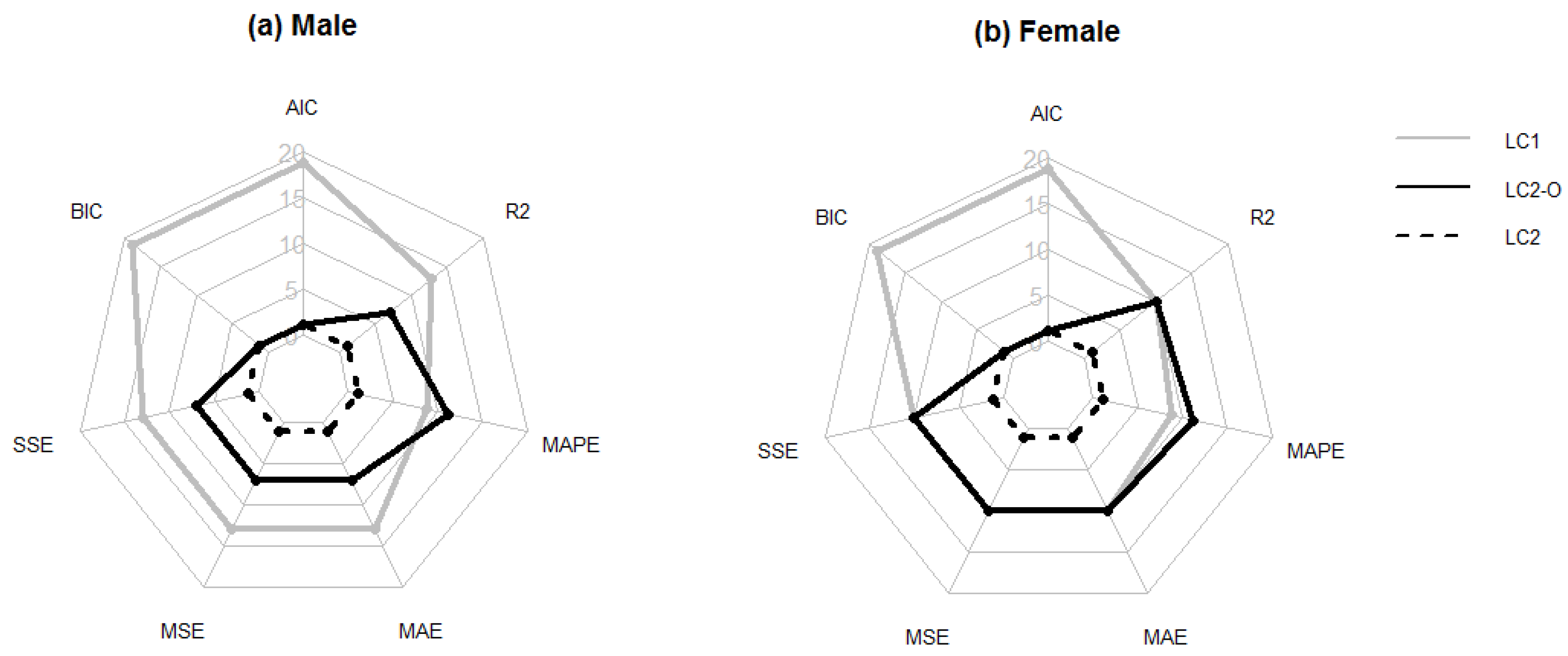
Figure 3 uses cobweb maps to show the number of times that each model yields the best result according to the seven criteria employed to measure the forecasting ability of the models. As seen in Figure 3, LC outperform the two alternative models when penalized measures are used to quantify the forecasting ability of the models. However, the results are more ambiguous when nonpenalized measures are applied.
5.4. Repeated Hold-Out
The second resampling method is the repeated hold-out that follows a similar procedure but considers the peculiarities of our sample.
- We randomly subdivide the sample into two subsets. Of the total data, 75% are used as the training subset, and the remaining 25% are the validation subset. Here, the data that correspond to the years 1990, 1991, 1992, 1993, 1994, 1995, 1996, 1998, 1999, 2000, 2001, 2002, 2003, 2005, 2006, 2009, 2011, 2013, 2014 and 2016 are used as the training set, and the data that correspond to the years 1997, 2004, 2007, 2008, 2010, 2012 and 2015 form the validation set.
- The three models are fitted with the training data set that obtains the corresponding estimates , and .
- Since the training set does not contain serialized data, we use the na.kalman function from the imputeTS library of [70] to estimate the missing values by using ARIMA time series models and obtain the values that corresponds to the years included in the validation set.
- Finally, we obtain the forecasted life tables of the years included in the validation set; then, the forecasting ability of the model is obtained by using the goodness-of-fit measures described in Section 4 that are applied to the validation dataset.
This procedure is repeated times, where the years that form the training and the validation sets are randomly changed. To obtain a global measure of the forecasting ability of each model, we proceed to calculate the average value by using Equation (5) for the 100 outcomes obtained for each country and sex in step 4.
Figure 4 summarizes the number of times that each model outperforms the other two alternatives according to the different criteria. When using this resampling method, the results are even more favorable to LC. The penalized measures choose LC for nearly all the countries, and even when nonpenalized measures are used, LC usually outperforms the other two models.
5.5. Leave-One-Out CV
Again, we have to adapt the methodology to apply it to a time series. In this case, the CV method undertakes the following steps.
- We use the first three years of the sample (1990, 1991 and 1992) as the training set. According to the tsCV function of the forecast library developed by [50], three is the minimum number of years necessary to fit the mortality models used in this study.
- We obtain the estimations of , and .
- By using the ARIMA model that best fits the values, a single forecast is obtained for the that correspond to the year 1993.
- Once these data are projected for 1993, we obtain the corresponding forecasted probabilities of death for all ages (from zero to 109 years), countries and populations, and we then proceed to calculate the forecasting ability measures with the 1993 data as the validation set.
This procedure is repeated 24 times. Each iteration incorporates an additional year into the training set and uses the data that correspond to the following year as the validation set.
A global measure of the forecasting ability of each model is calculated as the average of the 24 results obtained each time that the model is applied. These results, again, are shown in Figure 5 by using a cobweb graph where each vertex represents the number of times that a model produces the best result according to the seven measures used in this study. Again, we obtain more evidence in favor of LC even when using nonpenalized measures of the goodness-of-fit.
5.6. The 5-Fold CV
The fourth method that we apply in this analysis is the 5-fold CV, since we have 24 years, and it follows the process shown bellow.
- We proceed to subdivide the sample into six equally sized subsets, that include subset data from four consecutive years. The first subset consists of data from 1990 to 1994 and is used only as a training set. The second subset contains data from 1995 to 1998, the third subset contains data from 1999 to 2002, the fourth subset contains data from 2003 to 2006, the fifth subset contains data from 2007 to 2011 and the sixth subset contains data from 2012 to 2016.
- With the data that correspond to the period from 1990 to 1994, we obtain the estimations of , and .
- We fit the ARIMA model to the values of by obtaining projections for the values that correspond to the second subset (from 1995 to 1998) that is used as the validation set.
- Finally, we forecast the life tables for each country according to sex and age from 1995 to 1998, and we can then proceed to determine the different measures of the forecasting ability of the mortality models employed in this study.
This procedure is repeated by enlarging the training set each time by using the following sample subset and the next four years of data as the validation set. That is, the next iteration consists of using data from 1990 to 1998 as the training set and the data from 1999 to 2002 as the validation set, etc.
Again, the forecasting power of a model is obtained as the average of the results of each iteration. Figure 6 illustrates these outcomes for each forecasting ability measure and indicates the number of times that a model yields the best results for the 30 countries considered in this study. Those models located in outer places are the models with the best result for most countries. The outcomes confirm again that LC outperforms the two other models, thereby showing the convenience of using resampling methods for evaluating alternative mortality models.
6. Conclusions
This paper has described the usefulness and simplicity of resampling methods and a radial plotting technique called radar plotting for multivariate graphical data. Although they are commonly used in other fields such as business management and engineering, these methods have not found a foothold in the presentation of research results related to mortality forecasting models. This provides an essential opportunity for knowledge translation to the actuarial community.
We propose using resampling methods to evaluate the forecasting ability of three different mortality models. Additionally, it is important to mention that these methods are very suitable for evaluating the predictive ability of models, especially the cross-validation models. Specifically, cross-validation models are especially suitable for our sample size.
The main result is that overall, the LC model provides the best results independently of the resampling method used and the criterion used to measure the forecasting ability. This result is valid for both the male and female populations. Despite the simplicity of this model (with a smaller number of parameters), its forecasting ability is better than the two other models, which require the estimation of many more parameters. These results are particularly evident when penalized measures of accuracy are employed to evaluate the forecasting ability of the models. For both the AIC and the BIC, the LC model produces the best results. Even when using nonpenalized measures, LC provides better outcomes in most cases.
When we apply nonpenalized measures in the hold-out method, we do not find precise results regarging the “best” model. The hold-out is a traditional method. However, when we apply the other three resampling methods (repeated hold-out, LOOCV, and K-fold CV) and compare the results, the LC model produces the best results (the only case where the LC model produces the worst results is for females when applying the repeated hold-out method). Therefore, the resampling methods allow us to determine the best model.
Concerning the work of other authors, we should emphasize that many of them seek to find the best model that predicts mortality in Europe. In this paper, we make a general bibliographical review of the different criteria employed to measure the goodness-of-fit of mortality models. Additionally, we do not apply a single resampling method but rather test a battery of resampling methods such as cross-validation by using hold-out, leave-one-out and k-fold CV. In addition, we have specified how to apply the resampling methods when we have access to time series data.
Finally, we would like to note that although this paper conducts predictions only by using European life tables, the methodology can be extended to the life tables of any geographical area.
The influence of social relationships on the risk of mortality is comparable to that of well-established risk factors for mortality [71]. Social networks have generated enormous volumes of data about human interaction. Big data research, which includes to these large datasets, offers insight into many domains, especially complex and social network applications [72], that we suggest can be applied to human mortality.
Author Contributions
All authors contributed equally. All authors have read and agreed to the published version of the manuscript.
Funding
The research of David Atance was supported by a grant (Contrato Predoctoral de Formación Universitario) from the University of Alcalá. This work is partially supported by a grant from the MEIyC (Ministerio de Economía, Industria y Competitividad, Spain project ECO2017-89715-P).
Acknowledgments
We would like to express our sincere thanks to the anonymous reviewers for their careful review of the manuscript and valuable remarks.
Conflicts of Interest
The authors declare that they have no conflict of interest to report.
Appendix A
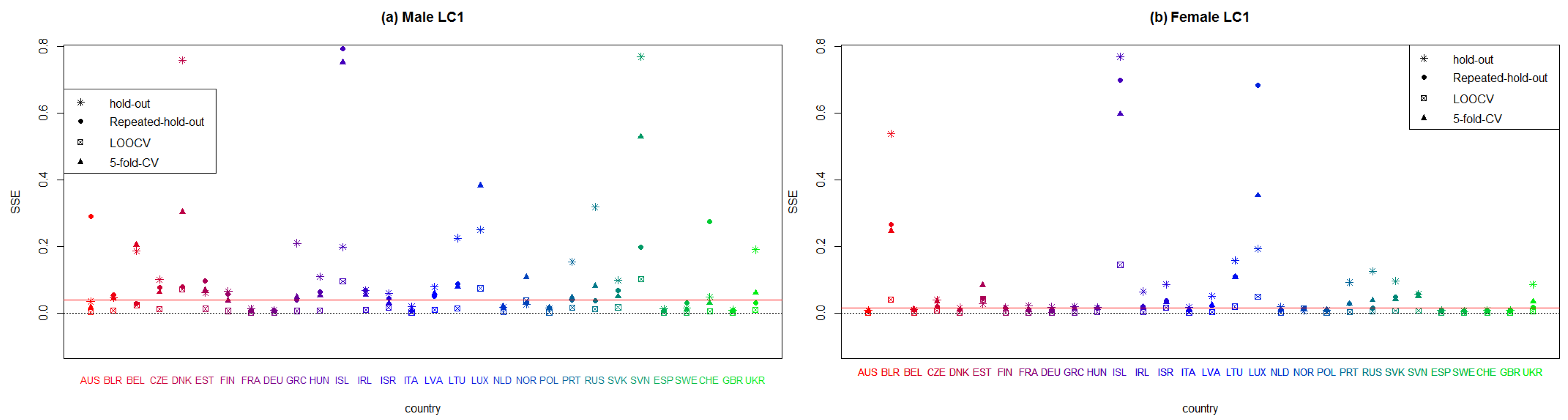
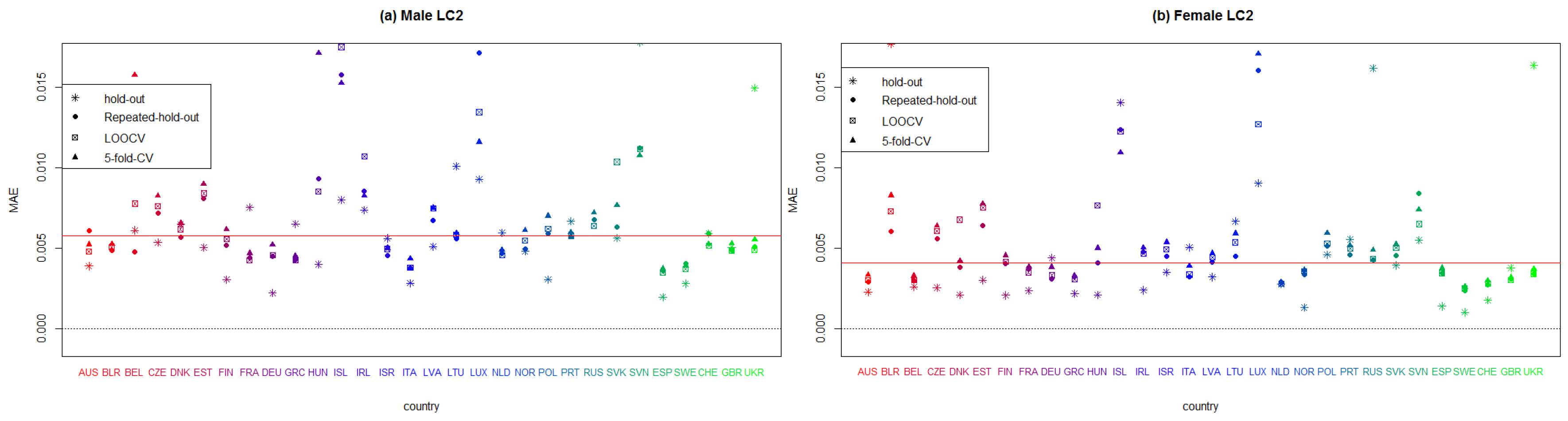
Figure A1, Figure A2, Figure A3, Figure A4, Figure A5 and Figure A6 display the values of the SSE and MAE measures in all European countries after applying every model considered in this paper, namely, the unifactorial Lee–Carter (LC), bifactorial Lee–Carter (LC2) and bifactorial Lee–Carter with orthogonalized parameters (LC2-O) models. We can therefore identify which model works best in each European country. The red line corresponds to the median, and each symbol corresponds to each resampling method. We do not employ penalized measures because we seek an individual analysis of the forecasting accuracy in the models. We include only the MAE and SSE for the sake of brevity although the rest of the criteria are available to the reader on request.
In Figure A1 and Figure A2, we can observe that LC fits best in countries where the exposure to risk is high. France, Germany, Italy, Netherlands, and Spain perform better than the rest of the countries for both sexes. Conversely, countries with a small population present the worst results (Belarus, Denmark, Iceland, Luxemburg and Slovenia). Suprisingly, the countries that were part of the former USSR have an inferior result in terms of goodness-of-fit.
In Figure A3 and Figure A4, we display the results that correspond to LC2. It can be seen that this model performs better for women than for men. Italy, Sweden, Spain, and the United Kingdom have the lowest error measure; meanwhile, Belarus, Iceland, Ireland, Luxemburg, Slovakia, and Slovenia yield the worst results. Finally, we exhibit the measures for LC2-O in Figure A5 and Figure A6. Once again, we observe that females produce smaller error measures than males. Denmark, Hungary, Iceland, Ireland, Lithuania, Luxemburg, Slovakia, and Slovenia are the European countries with the worst results, while Austria, France, Germany, Italy, Netherlands, Spain, Switzerland, and the United Kingdom produce the lowest values in the SSE and MAE. Clearly, whatever model is used to forecast mortality rates, the quality of the fitting is highly dependent on the population size and stability of mortality.
Figure A1.
Plot summarizing the sum of squares errors (SSE) of each European country that applies the unifactorial Lee–Carter model to males and females, according to every employed resampling method.
Figure A1.
Plot summarizing the sum of squares errors (SSE) of each European country that applies the unifactorial Lee–Carter model to males and females, according to every employed resampling method.

Figure A2.
Plot summarizing the mean absolute measure (MAE) of each European country that applies the unifactorial Lee–Carter model to males and females, according to every employed resampling method.
Figure A2.
Plot summarizing the mean absolute measure (MAE) of each European country that applies the unifactorial Lee–Carter model to males and females, according to every employed resampling method.

Figure A3.
Plot that summarizing the sum of squares errors (SSE) of each European country that applies bifactorial Lee–Carter model to males and females, according to every employed resampling method.
Figure A3.
Plot that summarizing the sum of squares errors (SSE) of each European country that applies bifactorial Lee–Carter model to males and females, according to every employed resampling method.

Figure A4.
Plot summarizing the mean absolute measure (MAE) of each European country that applies bifactorial Lee–Carter model to males and females, according to every employed resampling method.
Figure A4.
Plot summarizing the mean absolute measure (MAE) of each European country that applies bifactorial Lee–Carter model to males and females, according to every employed resampling method.

Figure A5.
Plot summarizing the sum of squares errors (SSE) of each European country that applies bifactorial Lee–Carter model with orthogonalized parameters to males and females, according to every employed resampling method.
Figure A5.
Plot summarizing the sum of squares errors (SSE) of each European country that applies bifactorial Lee–Carter model with orthogonalized parameters to males and females, according to every employed resampling method.

Figure A6.
Plot summarizing the mean absolute measure (MAE) of each European country that applies bifactorial Lee–Carter model with orthogonalized parameters to males and females, according to every employed resampling method.
Figure A6.
Plot summarizing the mean absolute measure (MAE) of each European country that applies bifactorial Lee–Carter model with orthogonalized parameters to males and females, according to every employed resampling method.

References
- Lee, R.D.; Carter, L.R. Modeling and forecast US mortality. J. Am. Stat. Assoc. 1992, 87, 659–671. [Google Scholar]
- Booth, H.; Maindonald, J.; Smith, L. Applying Lee—Carter under conditions of variable mortality decline. Popul. Stud. 2002, 56, 325–336. [Google Scholar] [CrossRef] [PubMed]
- Brouhns, N.; Denuit, M.; Vermunt, J.K. A Poisson log—Bilinear regression approach to the construction of projected lifetables. Insur. Math. Econ. 2002, 3, 373–393. [Google Scholar] [CrossRef] [Green Version]
- Lee, R.; Miller, T. Evaluating the performance of the Lee—Carter method for forecasting mortality. Demography 2001, 38, 537–549. [Google Scholar] [CrossRef] [PubMed]
- Cairns, A.J.G.; Blake, D.; Dowd, K. A two-factor model for stochastic mortality with parameter uncertainty: Theory and calibration. J. Risk Insur. 2006, 73, 687–718. [Google Scholar] [CrossRef]
- Cairns, A.J.G.; Blake, D.; Dowd, K.; Coughlan, G.D.; Epstein, D.; Ong, A.; Balevich, I. A quantitative comparison of stochastic mortality models using data from England and Wales and the United States. N. Am. Actuar. J. 2009, 13, 1–35. [Google Scholar] [CrossRef]
- Renshaw, A.E.; Haberman, S. Lee—Carter mortality forecasting with age-specific enhancement. Insur. Math. Econ. 2003, 33, 255–272. [Google Scholar] [CrossRef]
- Renshaw, A.E.; Haberman, S. A cohort-based extension to the Lee—Carter model for mortality reduction factors. Insur. Math. Econ. 2006, 38, 556–570. [Google Scholar] [CrossRef]
- Hainaut, D. A neural-network analyzer for mortality forecast. ASTIN Bull. J. IAA 2018, 48, 481–508. [Google Scholar] [CrossRef] [Green Version]
- Levantesi, S.; Pizzorusso, V. Application of machine learning to mortality modeling and forecasting. Risks 2019, 7, 26. [Google Scholar] [CrossRef] [Green Version]
- Pascariu, M.D.; Lenart, A.; Canudas-Romo, V. The maximum entropy mortality model: Forecasting mortality using statistical moments. Scand. Actuar. J. 2019, 2019, 661–685. [Google Scholar] [CrossRef]
- Śliwka, P.; Socha, L. A proposition of generalized stochastic Milevsky—Promislov mortality models. Scand. Actuar. J. 2018, 8, 706–726. [Google Scholar] [CrossRef]
- James, G.; Witten, D.; Hastie, T.; Tibshirani, R. An Introduction to Statistical Learning: With Application in R; Springer: New York, NY, USA, 2013. [Google Scholar]
- Lyons, M.B.; Keith, D.A.; Phinn, S.R.; Mason, T.J.; Elith, J. A comparison of resampling methods for remote sensing classification and accuracy assessment. Eur. Actuar. J. 2008, 208, 145–153. [Google Scholar] [CrossRef]
- Molinaro, A.M.; Simon, R.; Pfeiffer, R.M. Prediction error estimation: A comparison of resampling methods. Bioinformatics 2005, 21, 3301–3307. [Google Scholar] [CrossRef] [PubMed] [Green Version]
- Arlot, S.; Celisse, A. A survey of cross-validation procedures for model selection. Stat. Surv. 2010, 4, 40–79. [Google Scholar] [CrossRef]
- Stone, M. Cross-validatory choice and assessment of statistical predictions. J. R. Stat. Soc. Ser. B (Methodol.) 1974, 36, 111–133. [Google Scholar] [CrossRef]
- Bergmeir, C.; Hyndman, R.J.; Koo, B. A note on the validity of cross-validation for evaluating autoregressive time series prediction. Comput. Stat. Data Anal. 2018, 120, 70–83. [Google Scholar] [CrossRef]
- Hastie, T.; Tibshirani, R.; Friedman, J. The Elements of Statistical Learning; Springer Series in Statistics: New York, NY, USA, 2009. [Google Scholar]
- Efron, B. Bootstrap methods: Another look at the jackknife. Ann. Stat. 1979, 7, 1–26. [Google Scholar] [CrossRef]
- Brouhns, N.; Denuit, M.; Van Keilegom, I. Bootstrapping the Poisson log-bilinear model for mortality forecasting. Scand. Actuar. J. 2005, 3, 212–224. [Google Scholar] [CrossRef]
- D’Amato, V.; Haberman, S.; Piscopo, G.; Russolillo, M. Modelling dependent data for longevity projections. Insur. Math. Econ. 2012, 51, 694–701. [Google Scholar] [CrossRef]
- Debón, A.; Martínez-Ruiz, F.; Montes, F. Temporal evolution of mortality indicators: Application to spanish data. N. Am. Actuar. J. 2012, 16, 364–377. [Google Scholar] [CrossRef]
- Debón, A.; Montes, F.; Mateu, J.; Porcu, E.; Bevilacqua, M. Modelling residuals dependence in dynamic life tables: A geostatistical approach. Comput. Stat. Data Anal. 2008, 52, 3128–3147. [Google Scholar] [CrossRef]
- Koissi, M.C.; Shapiro, A.F.; Högnäs, G. Evaluating and extending the Lee—Carter model for mortality forecasting: Bootstrap confidence interval. Insur. Math. Econ. 2006, 38, 1–20. [Google Scholar] [CrossRef]
- Liu, X.; Braun, W.J. Investigating mortality uncertainty using the block bootstrap. J. Probab. Stat. 2010, 2010, 813583. [Google Scholar] [CrossRef] [Green Version]
- Efron, B.; Tibshirani, R.J. An Introduction to the Bootstrap. Monogr. on Stat. and Appl. Probab. 1993, 57, 1–436. [Google Scholar]
- Nordman, D.J.; Lahiri, S.N.; Fridley, B.L. Optimal block size for variance estimation by a spatial block bootstrap method. Indian J. Stat. 2007, 69, 468–493. [Google Scholar]
- Härdle, W.; Horowitz, J.; Kreiss, J.P. Bootstrap methods for time series. Int. Stat. Rev. 2003, 71, 435–459. [Google Scholar] [CrossRef] [Green Version]
- Bergmeir, C.; Benítez, J.M. On the use of cross-validation for time series predictor evaluation. Inf. Sci. 2012, 191, 192–213. [Google Scholar] [CrossRef]
- Debón, A.; Montes, F.; Sala, S. A comparison of parametric models for mortality graduation. Application to mortality data of the Valencia region (Spain). SORT Stat. Oper. Res. Trans. 2005, 29, 269–288. [Google Scholar]
- Booth, H.; Hyndman, R.J.; Tickle, L.; de Jong, P. Lee—Carter mortality forecasting: A multi-country comparison of variants and extensions. Demogr. Res. 2006, 15, 289–310. [Google Scholar] [CrossRef]
- Delwarde, A.; Denuit, M.; Eilers, P. Smoothing the Lee—Carter and Poisson log-bilinear models for mortality forecasting: A penalized log-likelihood approach. Stat. Model. 2007, 7, 29–48. [Google Scholar] [CrossRef]
- Debón, A.; Montes, F.; Puig, F. Modelling and forecasting mortality in Spain. Eur. J. Oper. Res. 2008, 189, 624–637. [Google Scholar] [CrossRef] [Green Version]
- Currie, I.D.; Durban, M.; Eilers, P.H.C. Smoothing and forecasting mortality rates. Stat. Model. 2004, 4, 279–298. [Google Scholar] [CrossRef]
- Chen, K.; Liao, J.; Shang, X.; Li, J.S.H. Discossion of “A Quantitative Comparison of Stochastic Mortality Models Using Data from England and Wales and the United States”. N. Am. Actuar. J. 2009, 13, 514–520. [Google Scholar] [CrossRef]
- Plat, R. On stochastic mortality modeling. Insur. Math. Econ. 2009, 45, 393–404. [Google Scholar] [CrossRef]
- Debón, A.; Martínez-Ruiz, F.; Montes, F. A geostatistical approach for dynamic life tables: The effect of mortality on remaining lifetime and annuities. Insur. Math. Econ. 2010, 47, 327–336. [Google Scholar] [CrossRef] [Green Version]
- Yang, S.S.; Yue, J.C.; Huang, H.C. Modeling longevity risks using a principal component approach: A comparison with existing stochastic mortality models. Insur. Math. Econ. 2010, 46, 254–270. [Google Scholar] [CrossRef]
- Haberman, S.; Renshaw, A. A comparative study of parametric mortality projection models. Insur. Math. Econ. 2011, 48, 35–55. [Google Scholar] [CrossRef] [Green Version]
- Mitchell, D.; Brockett, P.; Mendoza-Arriaga, R.; Muthuraman, K. Modeling and forecasting mortality rates. Insur. Math. Econ. 2013, 52, 275–285. [Google Scholar] [CrossRef]
- Cadena, M. Mortality Models based on the Transform log(−log x). arXiv 2015, arXiv:1502.07199. [Google Scholar]
- Danesi, I.L.; Haberman, S.; Millossovich, P. Forecasting mortality in subpopulations using Lee—Carter type models: A comparison. Insur. Math. Econ. 2015, 62, 151–161. [Google Scholar] [CrossRef]
- Yang, B.; Li, J.; Balasooriya, U. Cohort extensions of the Poisson common factor model for modelling both genders jointly. Scand. Actuar. J. 2016, 2, 93–112. [Google Scholar] [CrossRef]
- Neves, C.; Fernandes, C.; Hoeltgebaum, H. Five different distributions for the Lee—Carter model of mortality forecasting: A comparison using GAS models. Insur. Math. Econ. 2017, 75, 48–57. [Google Scholar] [CrossRef]
- Human Mortality Database. University of California, Berkeley (USA), and Max Planck Institute for Demographic Research (Germany). Available online: www.mortality.org (accessed on 7 August 2020).
- R Core Team. R: A Language and Environment for Statistical Computing; R Foundation for Statistical Computing: Vienna, Austria, 2018; Available online: https://www.R-project.org/ (accessed on 19 November 2019).
- Hunt, A.; Blake, D. Identifiability in age/period/cohort mortality models. Ann. Actuar. Sci. 2020. forthcoming. [Google Scholar] [CrossRef] [Green Version]
- Turner, H.; Firth, D. Generalized Nonlinear Models in R: An Overview of the Gnm Package. 2018. Available online: https://cran.r-project.org/package=gnm (accessed on 12 January 2020).
- Hyndman, R.J.; Khandakar, Y. Automatic time series forecasting: The forecast package for R. J. Stat. Softw. 2008, 26, 1–22. [Google Scholar]
- Lachenbruch, P.A.; Mickey, M.R. Estimation of error rates in discriminant analysis. Technometrics 1968, 10, 1–11. [Google Scholar] [CrossRef]
- Kohavi, R. A study of cross-validation and bootstrap for accuracy estimation and model selection. In Proceedings of the Fourteenth International Joint Conference on Artificial Intelligence, Montreal, QC, Canada, 20–25 August 1995; Morgan Kaufmann: San Francisco, CA, USA, 1995; pp. 1137–1143. [Google Scholar]
- Torgo, L. Data mining with R: Learning with case studies. In Data Mining and Knowledge Discovery Series; Chapman and Hall/CRC: Boca Raton, FL, USA, 2010. [Google Scholar]
- Tashman, L.J. Out-of-sample tests of forecasting accuracy: An analysis and review. Int. J. Forecast. 2000, 16, 437–450. [Google Scholar] [CrossRef]
- Diaz, G.; Ana, D.; Giner-Bosch, V. Mortality forecasting in Colombia from abridged life tables by sex. Genus 2018, 74, 15. [Google Scholar] [CrossRef]
- Ahcan, A.; Medved, D.; Olivieri, A.; Pitacco, E. Forecasting mortality for small populations by mixing mortality data. Insur. Math. Econ. 2014, 54, 12–27. [Google Scholar] [CrossRef]
- Atance, D.; Balbás, A.; Navarro, E. Constructing dynamic life tables with a single factor model. In Documentos de trabajo IAES; Instituto Universitario de Análisis Económico y Social Universidad de Alcalá: Madrid, Spain, 2019; Volume 9, pp. 1–45. [Google Scholar]
- Forsythe, A.; Hartigan, J.A. Efficiency of confidence intervals generated by repeated subsample calculations. Biometrika 1970, 57, 629–639. [Google Scholar] [CrossRef]
- Burman, P. A comparative study of ordinary cross-validation, v-fold cross-validation and the repeated learning-testing methods. Biometrika 2002, 76, 503–514. [Google Scholar] [CrossRef] [Green Version]
- Shao, J. Linear model selection by cross-validation. J. Am. Stat. Assoc. 1993, 88, 486–494. [Google Scholar] [CrossRef]
- Hyndman, R.J.; Athanasopoulos, G. Forecasting: Principles and Practice; OTexts: Melbourne, Australia, 2018. [Google Scholar]
- Li, H.; O’Hare, C. Mortality Forecasting: How far back should we look in time? Risks 2019, 7, 22. [Google Scholar] [CrossRef] [Green Version]
- Breiman, L.; Spector, P. Submodel selection and evaluation in regression: The X-random case. Int. Stat. Rev. 1992, 60, 291–319. [Google Scholar] [CrossRef]
- Akaike, H. A new look at the statistical model identification. IEEE Trans. Autom. Control 1974, 6, 716–723. [Google Scholar] [CrossRef]
- Schwarz, G. Estimating the dimension of a model. Ann. Stat. 1978, 6, 461–464. [Google Scholar] [CrossRef]
- Hunt, A.; Blake, D. A general procedure for constructing mortality models. N. Am. Actuar. J. 2014, 18, 116–138. [Google Scholar] [CrossRef]
- Riffe, T. Reading Human Fertility Database and Human Mortality Database Data into R; TR-2015-004; MPIDR: Rostock, Germany, 2015. [Google Scholar]
- Hyndman, R.J.; Booth, H.; Tickle, L.; Maindonald, J. Demography: Forecasting Mortality, Fertility, Migration and Population Data. R Package Version 1.21; 2010; Available online: http://CRAN.R-project.org/package=demography (accessed on 12 January 2020).
- Nakazawa, M. fmsb: Functions for Medical Statistics Book with Some Demographic Data. R Package Version 0.6.3; 2018; Available online: https://CRAN.R-project.org/package=fmsb (accessed on 12 January 2020).
- Moritz, S.; Bartz-Beielstein, T. imputeTS: Time Series Missing Value Imputation in R. R J. 2017, 9, 207–2018. Available online: https://journal.r-project.org/archive/2017/RJ-2017-009/index.html (accessed on 12 January 2020). [CrossRef] [Green Version]
- Holt-Lunstad, J.; Smith, T.B.; Layton, J.B. Social relationships and mortality risk: A meta-analytic review. PLoS Med. 2010, 7, e1000316. [Google Scholar] [CrossRef]
- Thai, M.T.; Wu, W.; Xiong, H. Big Data in Complex and Social Networks; Chapman and Hall/CRC Press: London, UK, 2016. [Google Scholar]
Figure 1.
A schematic display of the employed resampling methods for an embedded time series. The training set, validation set and omitted set are shown in gray, white and black, respectively.
Figure 1.
A schematic display of the employed resampling methods for an embedded time series. The training set, validation set and omitted set are shown in gray, white and black, respectively.

Figure 2.
A schematic display of the employed resampling methods for nonembedded time series. The training sets and validation sets are shown in gray and white, respectively.
Figure 2.
A schematic display of the employed resampling methods for nonembedded time series. The training sets and validation sets are shown in gray and white, respectively.

Figure 3.
Radar graph summarizing the number of countries for which each model (LC, LC2, and LC2-O) achieves the best forecasting ability according to the hold-out method for males (a) and females (b).
Figure 3.
Radar graph summarizing the number of countries for which each model (LC, LC2, and LC2-O) achieves the best forecasting ability according to the hold-out method for males (a) and females (b).

Figure 4.
Radar graph summarizing the number of countries for which each model (LC, LC2, and LC2-O) achieves the best forecasting ability according to the repeated hold-out method for males (a) and females (b).
Figure 4.
Radar graph summarizing the number of countries for which each model (LC, LC2, and LC2-O) achieves the best forecasting ability according to the repeated hold-out method for males (a) and females (b).

Figure 5.
Radar graphs summarizing the number of countries for which each model (LC, LC2, and LC2-O) achieves the best forecasting ability according to the leave-one-out method for males (a) and females (b).
Figure 5.
Radar graphs summarizing the number of countries for which each model (LC, LC2, and LC2-O) achieves the best forecasting ability according to the leave-one-out method for males (a) and females (b).

Figure 6.
Radar graph that summarizing the number of countries for which each model (LC, LC2, and LC2-O) achieves the best forecasting ability according to the 5-fold CV method for males (a) and females (b).
Figure 6.
Radar graph that summarizing the number of countries for which each model (LC, LC2, and LC2-O) achieves the best forecasting ability according to the 5-fold CV method for males (a) and females (b).


Table 1.
Summary of goodness-of-fit measures.
| Paper | Measure of Goodness Fit | Mortality Models | Selected Model |
|---|---|---|---|
| [31] | Gompertz–Makeham | Logit–Gompertz–Makeham | |
| MAPE | Logit–Gompertz–Makeham | ||
| Heligman–Pollard–2law | |||
| [32] | MAE | LC1/LM | BMS with small differences |
| ME | BMS/HU | ||
| LC-smooth | |||
| [33] | AIC | LC1-Negative Binomial | LC1-Negative Binomial |
| BIC | LC1-Poisson | ||
| [24] | MAPE | LC1-Logit/LC2-Logit | MP |
| MSE | Median Polish (MP) | ||
| [34] | MAPE | LC1-SVC/LC1-GLM | LC2 |
| MSE | LC1-ML/LC2-SVD | ||
| LC2-GLM/LC2-ML | |||
| [6] | BIC | LC1/LC2-Cohort | LC2-Cohort |
| APC/M5 | M8 | ||
| [35] | |||
| M6/M7/M8 | |||
| [36] | SSE | M5-Logit | M5-Logit |
| M5-Log/M5-Probit | |||
| [37] | BIC | [37] model | [37] model |
| LC1/M7/M5 | |||
| LC2-Cohort | |||
| [35] model | |||
| [38] | Deviance | LC1/LC1-res | LC-APC |
| MSE | LC2/LC2-res | ||
| MAPE | LC-APC/LC-APC-res | ||
| MP/MP-res | |||
| MP-APC/MP-APC-res | |||
| [39] | MAPE | LC1/APC1 | [39] model |
| BIC | APC2/CBD | ||
| [39] model | |||
| [40] | AIC | LC1/ | M7/M8/ |
| BIC | M/LC2 | ||
| HQC | M5/M6 | ||
| M7/M8 | |||
| [41] | RSSE | [41] model | RH |
| LC1/RH | [41] | ||
| BIC | / | ||
| [37] model | |||
| [42] | MSE | LC1/CBD | [42] model |
| MAPE | [42] model | ||
| [43] | MAPE | P-Double-LC2/M-Double-LC2 | P-Common-LC2 |
| AIC | P-Common-LC2/M-Common-LC1 | ||
| BIC | P-Simple-LC1/M-Simple-LC1 | ||
| MAPE | P-Division-LC1/M-Division-LC1 | ||
| P-One-LC1/M-One-LC1 | |||
| [44] | BIC | PCFC | PCFC |
| MAPE | PCFM | ||
| [45] | AIC | GAS Poisson/GAS Binomial | GAS Negative Binomial |
| MAPE | GAS Negative Binomial | ||
| GAS Gaussian/GAS Beta |
Table 2.
List of the Lee–Carter models used in this study, with the acronyms, parameter constraints and equations.
Table 2.
List of the Lee–Carter models used in this study, with the acronyms, parameter constraints and equations.
| Label Model | Parameter Constraints | Formula |
|---|---|---|
| LC | ||
| LC2 | ||
| LC2-O | ||
© 2020 by the authors. Licensee MDPI, Basel, Switzerland. This article is an open access article distributed under the terms and conditions of the Creative Commons Attribution (CC BY) license (http://creativecommons.org/licenses/by/4.0/).
Share and Cite
MDPI and ACS Style
Atance, D.; Debón, A.; Navarro, E. A Comparison of Forecasting Mortality Models Using Resampling Methods. Mathematics 2020, 8, 1550. https://0-doi-org.brum.beds.ac.uk/10.3390/math8091550
AMA Style
Atance D, Debón A, Navarro E. A Comparison of Forecasting Mortality Models Using Resampling Methods. Mathematics. 2020; 8(9):1550. https://0-doi-org.brum.beds.ac.uk/10.3390/math8091550
Chicago/Turabian StyleAtance, David, Ana Debón, and Eliseo Navarro. 2020. "A Comparison of Forecasting Mortality Models Using Resampling Methods" Mathematics 8, no. 9: 1550. https://0-doi-org.brum.beds.ac.uk/10.3390/math8091550
Note that from the first issue of 2016, this journal uses article numbers instead of page numbers. See further details here.