Ridge Fuzzy Regression Modelling for Solving Multicollinearity


1
Department of Statistics, North Carolina State University, Raleigh, NC 27695, USA
2
Department of Applied Mathematics, Hanyang University, Gyeonggi-do 15588, Korea
*
Author to whom correspondence should be addressed.
Mathematics 2020, 8(9), 1572; https://0-doi-org.brum.beds.ac.uk/10.3390/math8091572
Submission received: 14 August 2020
/
Revised: 5 September 2020
/
Accepted: 10 September 2020
/
Published: 12 September 2020
(This article belongs to the Special Issue Applications of Fuzzy Optimization and Fuzzy Decision Making)
Abstract
:This paper proposes an -level estimation algorithm for ridge fuzzy regression modeling, addressing the multicollinearity phenomenon in the fuzzy linear regression setting. By incorporating -levels in the estimation procedure, we are able to construct a fuzzy ridge estimator which does not depend on the distance between fuzzy numbers. An optimized -level estimation algorithm is selected which minimizes the root mean squares for fuzzy data. Simulation experiments and an empirical study comparing the proposed ridge fuzzy regression with fuzzy linear regression is presented. Results show that the proposed model can control the effect of multicollinearity from moderate to extreme levels of correlation between covariates, across a wide spectrum of spreads for the fuzzy response.
1. Introduction
Often times in practical applications, the available data may not always be precise. The researcher may be only accessible to minimum and maximum values of data. Sometimes the data may not even be given in numbers. For instance, consider linguistics data such as “young”, “tall”, or “high”, and medicine data such as “healthy” and “not healthy”. In such cases where the given data are imprecise and vague, classical representation of numbers may be insufficient. The fuzzy set theory introduced by Zadeh [1,2] can handle such uncertainty in data. In the view of fuzzy set theory, uncertain data are what is called fuzzy. Fuzzy data are prevalent in various fields such as linguistics, survey, medicine and so forth [3,4,5,6,7]. The development of fuzzy set theory has led to statistical methods for analyzing fuzzy data. When the measure of indeterminacy is needed, the neutrosophic set introduced by Smarandache [8] considered the measure of indeterminacy in addition to the fuzzy set. The neutrosophic statistics based on the the neutrosophic set can be applied for the analysis of the data when data are selected from the population with uncertain, fuzzy, and imprecise observations [9].
In 1982, Tanaka et al. [10] proposed the fuzzy linear regression model which generalizes the usual linear regression model to fuzzy data. Fuzzy regression models have been since then widely used to analyze fuzzy data [11,12,13,14,15,16].
In classical linear regression models, the multicollinearity phenomenon is frequently observed in which two or more explanatory variables are highly linearly related. Common examples of collinear covariates are: a person’s height and weight, a person’s level of education, gender, race, and starting salary. When multicollinearity occurs, the least squares estimator may not be obtainable or be subject to very high variance. Once the researcher identifies the collinear variables, there are several techniques the researcher can use to handle multicollinearity. Among these techniques, the two most widely used approaches are lasso regression and ridge regression. Lasso regression developed by Tibshirani [17] and ridge regression developed by Hoerl and Kennard [18] improve model performance by adding a penalty term to the classical linear regression model. Both methods aim to shrink the model parameters towards zero. This induces a sparse model which increases the model bias, but decreases the model variance even more, thus improving overall performance. Ridge regression decreases the parameters of low contributing variables towards zero, but not exactly to zero, and stabilizing the parameter variance of the least squares estimator in the presence of multicollinearity. Lasso regression sets the model parameters exactly to zero, removing low contributing variables as well as improving model fitting. However, sometimes the researcher may want to include all the available covariates in the model without having to reduce the dimension of the data. In such cases, ridge regression is preferred to lasso regression.
Similar to classical linear regression models, multicollinearity occurs frequently in fuzzy linear regression models as well, causing problems in the estimation procedure. Often times the number of covariates is not particularly large for fuzzy data. Consequently, dropping any explanatory variables may not be an option. As in the classical statistical setting, we prefer to use ridge regression to lasso regression to handle multicollinearity in such datasets. In this paper, we incorporate fuzzy set theory with ridge regression developed by Hoerl and Kennard [18] to handle multicollinearity observed in fuzzy data. Only some works have suggested ridge estimation methods for fuzzy linear regression, and are limited to obtaining fuzzy ridge estimators which are dependent on the distance between fuzzy numbers [19,20,21]. We instead propose an -level estimation algorithm for ridge fuzzy regression modelling. The proposed algorithm is an extension of the ridge regression model introduced in Choi et al. [22]. By applying -levels to the estimation procedure, we are able to construct a fuzzy ridge estimator which does not depend on the distance between fuzzy numbers. Simulation experiments show the proposed ridge fuzzy regression model can solve moderate to severe degrees of multicollinearity across a wide range of spreads for the fuzzy response. An empirical study using Tanaka’s house prices data [10] with multicollinearity, the most widely applied data set in the fuzzy linear regression literature, is conducted to demonstrate the practical implementations.
The rest of this paper is organized as follows. Section 2 introduces key definitions and results from fuzzy set theory. Section 3 describes the classical ridge regression, followed by a step-by-step procedure for the proposed -level estimation algorithm of ridge fuzzy regression modeling. Section 4 and Section 5 illustrates the performance of the model with simulation studies and a numerical example, respectively. Section 6 concludes the paper.
2. Fuzzy Numbers
A fuzzy set is a set of ordered pairs where is a membership function which represents the degree of membership of x in a set A. Please note that when A is a crisp (classical) set, its membership function can take only the values one or zero depending on whether or not x does or does not belong to A. In this case, reduces to the indicator function of a set A. For any in , the -level set of a fuzzy set A is a crisp set which contains all the elements in X with membership value in A greater than or equal to . The -level set of a fuzzy set A can also be represented by . Here and are the left and right end-points of the -level set, respectively. Zadeh’s [23] resolution identity theorem states that a fuzzy set can represented by its membership function or by its -level set. Let A be a fuzzy number with membership function and -cut . Then we have .
A fuzzy number is a normal and convex subset of the real line R with bounded support. The support of a fuzzy set A is defined by . The following parametric class of fuzzy numbers, the so-called -fuzzy numbers denoted by , is often used as a special case:
where are fixed, left-continuous, and non-increasing functions with , and . L and R are called left and right shape functions of A, respectively. is the mean value of A, and are each the left and right spreads of A. The spreads and represent the fuzziness of the fuzzy number and can be symmetric or asymmetric. If , the -fuzzy number becomes a precise real number with no fuzziness. Thus, a precise real number can be considered to be a special case of a fuzzy number. For a precise observation , its corresponding membership function is .
In the fuzzy set theory, triangular and trapezoidal fuzzy numbers are special cases of -fuzzy numbers and are used extensively [24]. The membership function of a triangular fuzzy number is given by
where , and are the left end-point, mid-point, and right end-point, respectively.
3. Ridge Fuzzy Regression
In this section, we propose the -level estimation algorithm for the proposed ridge fuzzy regression model. This algorithm modifies the method based on Choi et al. [22] to estimate the fuzzy parameters. The term -level estimation indicates that our algorithm uses -levels to describe fuzzy data. By using -level, we are able to develop a ridge fuzzy estimator which is not restricted to the distance between fuzzy numbers. We first briefly examine the original formulation of ridge regression model for crisp data.
3.1. Ridge Regression
Given a data set , a multiple linear regression model assumes that the relationship between a dependent variable , and a set of explanatory variables , is linear. The model takes the form
or written alternatively in matrix notation as . A vector is a vector of observations on the dependent variable, is a matrix of explanatory variables, is a vector of regression coefficients to be estimated, and is a vector of error terms. The standard estimator for is the least squares estimator defined by
In the presence of multicollinearity, i.e., in state of extreme correlations among the explanatory variables is poorly determined and susceptible to high variance. Thus, we may deliberately bias the regression coefficient estimates so as to control their variance. In this manner, the ridge regression estimator was introduced by Hoerl and Kennard [18] as a penalized least squares estimator. It is achieved by minimizing the residual sum of squares (RSS) subject to a constraint on the size of the estimated coefficient vector [25]:
Here is a shrinkage parameter which controls the size of the coefficients. The larger the value of , the greater the amount of shrinkage, and we have coefficients close to zero. The smaller the value of is close to 0, we obtain the least squares solutions. Please note that by convention the input matrix is assumed to be standardized and is assumed to be centered before solving RSS(). The ridge regression solution is
where is the identity matrix. The shrinkage parameter is usually selected via K-fold cross validation. Cross validation is a simple and powerful tool often used to calculate the shrinkage parameter and the prediction error in ridge regression. The entire dataset is divided into K parts, and trains the model on all but the kth part. The model is validated on the part, iterating for all . The choice of K is or in general.
3.2. Ridge Fuzzy Regression Algorithm
Let us consider a set of observations
where the dependent variable , and the explanatory variables , are triangular fuzzy numbers. We assume a linear relationship between the dependent and explanatory variables:
where are the fuzzy regression parameters and are the fuzzy error terms. ⊕ and ⊙ represent addition and multiplication between two fuzzy numbers, respectively. Often the N equations are stacked together and written in matrix notation as
For more details on arithmetic operations between fuzzy numbers, see [10,26]. Please note that the above fuzzy variables can be symmetric or asymmetric, and be extended to various forms such as normal, parabolic, or square root fuzzy data. Since crisp sets are a special case of fuzzy sets, fuzzy inputs and fuzzy outputs, or fuzzy inputs and crisp outputs combinations are also possible. For illustration purposes, in this section, we present our ridge fuzzy regression model using triangular membership functions.
We divide the given data into training and test sets. The model is computed from the training set , and later its performance is evaluated on the test set . Note again that N is the total number of observations, n is the number of observations for the training set, and m is the number of observations for the test set, such that . We fit our ridge fuzzy regression model on the training set by the following estimation algorithm:
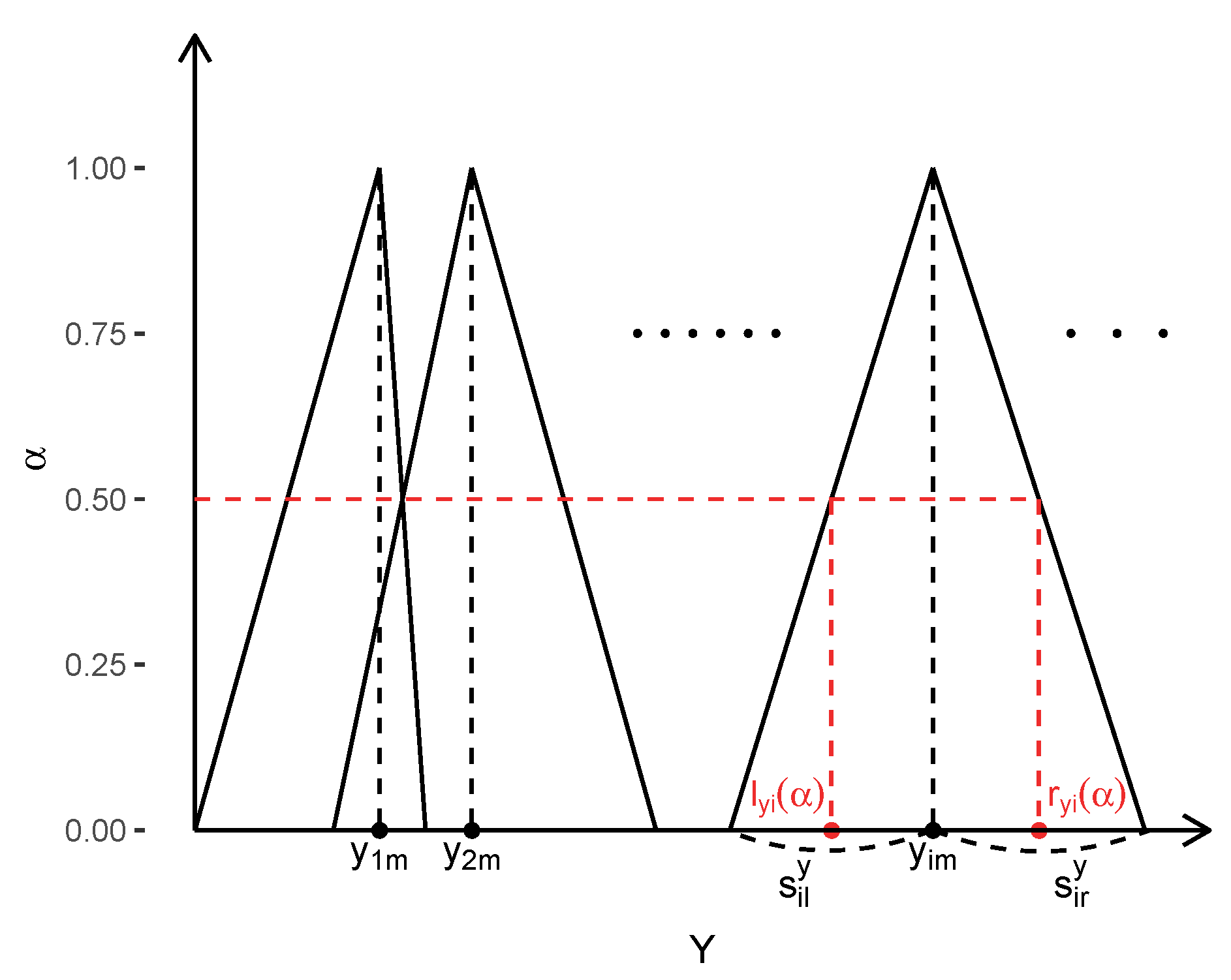
Step 1: Create -level sets of the triangular fuzzy input and output as illustrated in Figure 1. For any -level in ,
where are the left and right spreads of the dependent and explanatory variables, respectively. The -levels are denoted by the sequence for some K with .
Step 2: Perform ridge regression of on for each . Find the intermediate estimators and of and by minimizing the following respective ridge loss functions (see Figure 2).
We assume the endpoints of the -level set of has been centered and the endpoints of -level set of has been standardized as is by convention in classical ridge regression [25].
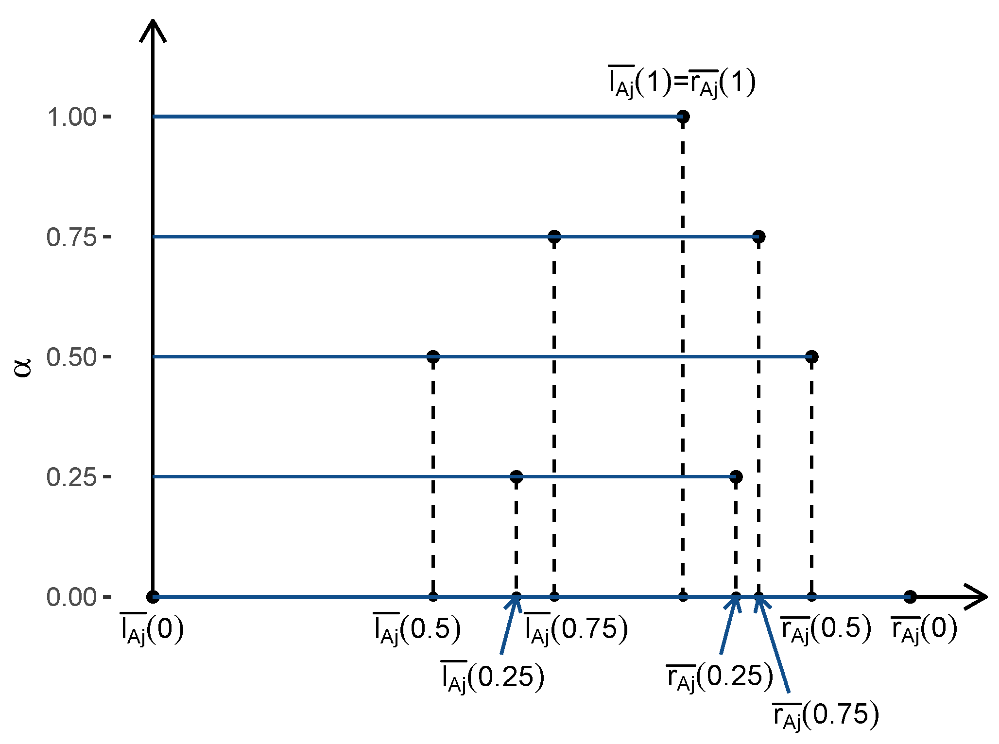
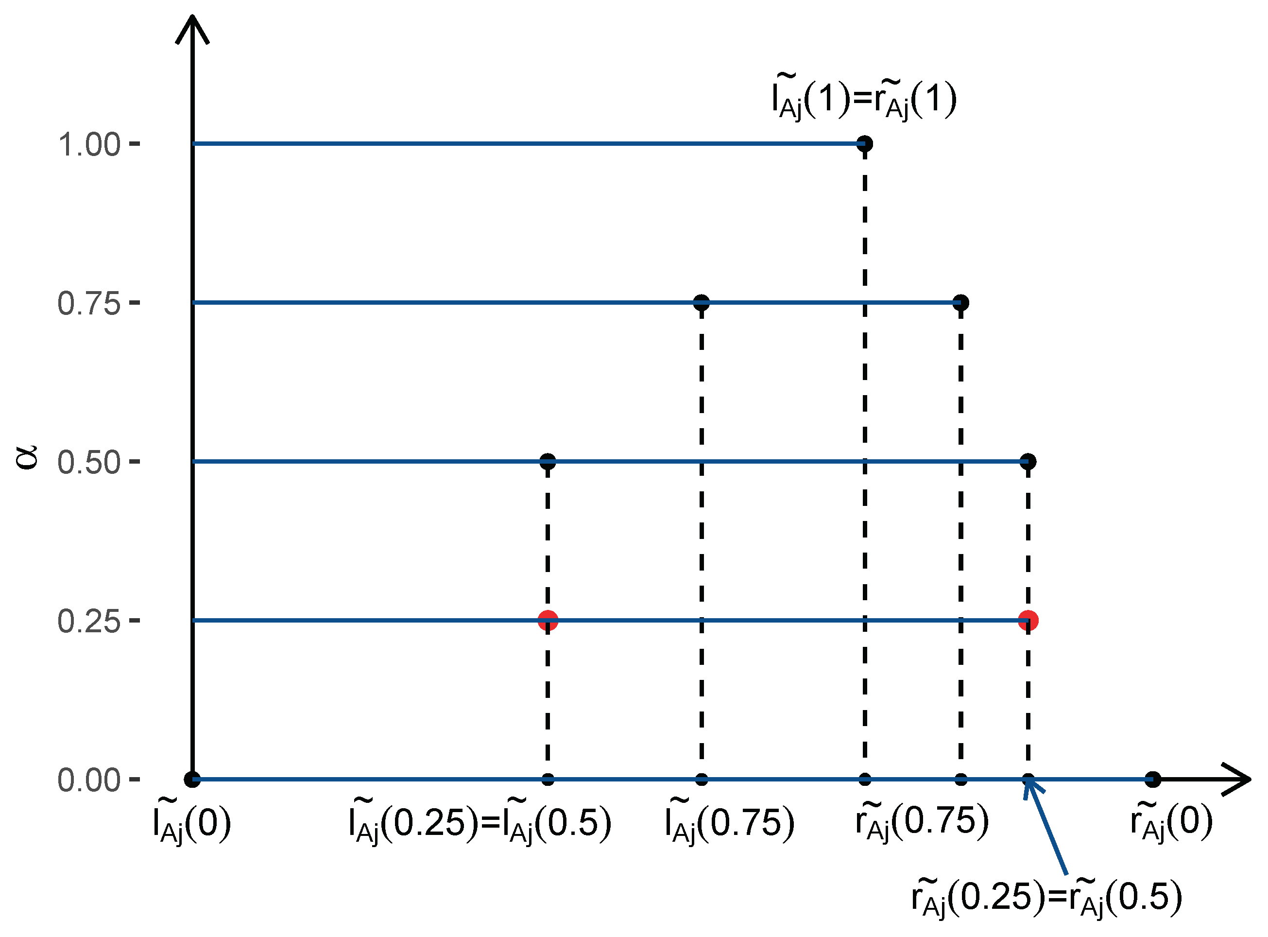
Step 3: Obtain the estimators and of and by modifying the intermediate estimators and so that the estimated coefficients form the membership function of a triangular fuzzy number. For this the following operations are performed (see Figure 3).
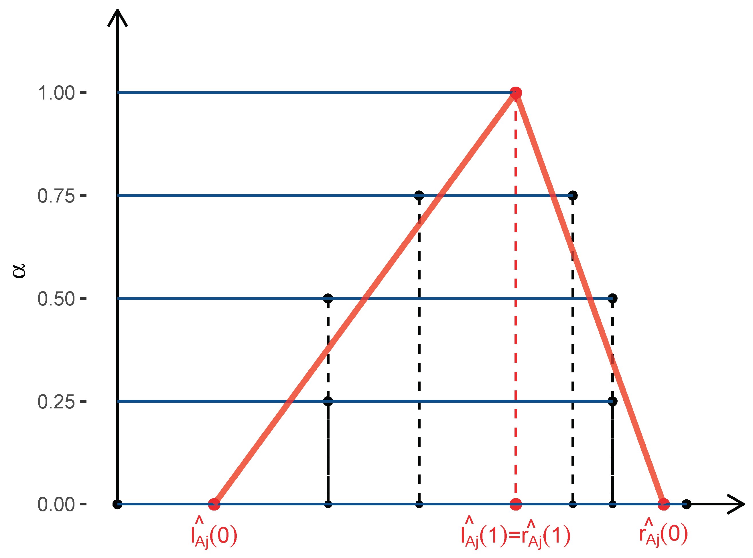
Step 4: Estimate the triangular fuzzy coefficient and its membership function by fitting a linear regression line through and for , respectively. A constraint is given so that satisfy the condition of (see Figure 4).
Step 5: Symmetric fuzzy inputs or outputs do not always guarantee that the estimated membership function will also be symmetric. To reduce the difference between the true values with the fitted values we consider the following candidates:
or
where is chosen as , or
where is chosen as .
We present two performance criteria based on Diamond’s fuzzy distance measure [27] to evaluate the proposed fuzzy estimators. Denote the dependent variable as , , and its predicted value as , . Here n is the number of observations for the training set. We defined (root mean square error for fuzzy numbers) and (mean absolute percentage error for fuzzy numbers) as below.
Compute the for each of the membership functions, then select the one which minimizes the criterion.
Step 6: Repeat Steps 1–5 for selected -level sequences with equally spaced between 0 and 1. Choose the optimal set of -levels which minimizes . Finally, compute the fuzzy ridge coefficient estimate based on that selected sequence.
4. Simulation Study
A simulation study was conducted to illustrate the performance of the proposed ridge fuzzy regression model in the presence of multicollinearity. Simulation results are compared with the fuzzy linear regression model with varying degrees of correlation. The fuzzy least squares estimator is obtained by setting the tuning parameter as zero in Step 2 of Section 3.2.
We generated observations for each of the crisp explanatory variables. The number of data dimensions is in line with commonly found fuzzy data. Following Gibbons [28], the explanatory variables are generated by
where is a given constant and are generated from independent normal distributions with mean 50 and variance 1. Here are assumed to be non-negative so as to reflect the non-negative characteristics of real world fuzzy data. The degree of linear association between explanatory variables is controlled via , where in this case is the correlation between any two explanatory variables is . Three different sets of correlation are considered corresponding to . Each value of stands for moderate, high, and very high correlation between the variables. Observations on the fuzzy dependent variable are generated by
where are generated from independent normal distributions with mean 0 and variance . Four values of are investigated in this study: 0.5, 1, 1.5, and 2. Large values of correspond to bigger variation in the spreads of the fuzzy dependent variable. the vector of left spreads and the vector of right spreads are determined by
Cases of asymmetric spreads, , and symmetric spreads, are also compared. The supposed parameters of the model are: . In order to analyze the effects of factors and , we controlled for the effects of varying -level sequences in Step 6 of Section 3.2. For both models we fixed the -level sequence as (0, 0.25, 0.5, 0.75, 1).
200 replicates for each scenario are generated. The explanatory variables and the fuzzy coefficients remain fixed, while the error terms and hence the fuzzy dependent variable changes. We separated the simulated data into training and test sets. Once the ridge fuzzy regression model and the fuzzy linear regression model are fit to the training data, and are computed from the test set for replicates. Let and be the performance measures when the fuzzy model is applied to the replicate t. The following quantities are then computed for each fuzzy estimator:
In addition, we fit the ridge regression model and the linear regression model on the mid-point of our training data for comparison with fuzzy methods. The test Ave. RMSE and Ave. MAPE values of 200 replicates are recorded for both models. The output from numerical experiments is suggested below in Table 1, Table 2, Table 3, Table 4, Table 5 and Table 6. Measures of performance are summarized for all combinations of factors and whether the fuzzy output is symmetric or not. The following remarks can be made on the basis of Table 1, Table 2, Table 3, Table 4, Table 5 and Table 6:
- Ave. RMSE and Ave. MAPE do not depend on whether the spreads are symmetric or not as they are computed from the mid-points of the generated data. Ridge regression achieves smaller Ave. RMSE than linear regression in all cases. Ridge regression achieves smaller or nearly equal Ave. MAPE with linear regression in all cases. If the Ave. RMSE of ridge regression is smaller than linear regression a similar pattern is observed for values. This relationship is observed for Ave. MAPE and as well.
- increases as increases for both models. As and increases, the difference between ridge fuzzy regression and fuzzy linear regression increases as well. values are larger when the spreads are symmetric. In all scenarios, ridge fuzzy regression values almost always outperform those of fuzzy linear regression.
- exhibit near identical patterns with . For both ridge fuzzy regression and fuzzy linear regression, is larger for bigger values. The difference between the two models increases as and increases. When the fuzzy dependent variable is symmetric the values are larger than when it is asymmetric. is in general lower for ridge fuzzy regression than fuzzy linear regression for all and combinations and asymmetric, symmetric outputs.
5. Empirical Study
In this section, we demonstrate the performance of the proposed ridge fuzzy regression model on an illustrative example taken from Tanaka [10]. The performance of the ridge fuzzy regression estimator is compared with the fuzzy least squares estimator for crisp explanatory variables and a fuzzy dependent variable. The linear regression fuzzy model from Tanaka [10] is further compared to illustrate the performance of the ridge fuzzy regression model. For both the ridge fuzzy regression and the linear fuzzy model, the -level sequences , for some r and K are chosen as candidates for Step 6 of the estimation algorithm in Section 3.2. The list of -level sequences is presented in Table 7.
Example: House Prices Data
Tanaka et al. [10] presents a data set concerning the price mechanism of prefabricated houses. The relationship between five crisp inputs (rank of material, first floor space (m2), second first floor space (m2), number of rooms and number of Japanese-style rooms) and a fuzzy output (house price) is investigated. The complete data is shown in Table 8. The fitted values for the ridge fuzzy model and the linear fuzzy model is shown in Table 9. Results show the predicted values from the ridge fuzzy regression more accurately describes the original data than fuzzy linear regression. This is again clarified in Figure 5. In the triangular fuzzy plot of the observed and fitted values, a comparison of the two models is shown. The black triangles correspond to the observed values, the red triangles in Figure 5a to the ridge fuzzy fitted values, and the blue triangles in Figure 5b to the fuzzy linear fitted values. Both methods estimated the mid-points of the fuzzy dependent variable well. The spreads however, are shorter for the proposed ridge fuzzy regression than the other. The fitted equation for the ridge fuzzy regression is given by
and for the fuzzy linear regression, the fitted equation is
Please note that the fitted equation for the linear regression fuzzy model shown in Tanaka et al. [10] is
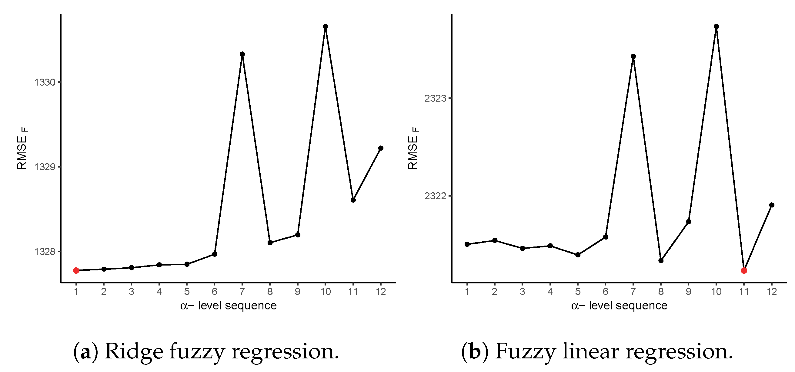
An analysis of the -level sequences used in Step 6 of the estimation algorithm is presented in Figure 6. The -level sequence which minimizes was chosen as the optimal -level sequence for each of the models. The red dots in Figure 6a,b each indicate the chosen -level sequence based on . For the ridge fuzzy regression, , with was chosen. In the case of fuzzy linear regression, was selected.
In Table 10 the performance measures and ridge fuzzy regression are compared with the fuzzy linear regression model and the linear regression fuzzy model from Tanaka et al. [10]. Clearly both measures are greatly reduced for the ridge fuzzy regression compared to the other models, suggesting that the proposed ridge fuzzy regression model provides a better fit of the data in comparison to the two methods.
6. Conclusions
This paper proposes an -level estimation algorithm for ridge fuzzy regression modeling, extending the ridge regression model introduced in Choi et al. [22]. As shown in simulation studies and an empirical study, the proposed ridge fuzzy regression model can handle fuzzy data sets with crisp inputs and triangular fuzzy outputs. The same procedure is available with fuzzy inputs and fuzzy outputs, or fuzzy inputs and crisp outputs. In previous works, estimation methods for ridge fuzzy regression depend on the distance between fuzzy numbers. By incorporating -levels to ridge fuzzy regression, we are able to construct the ridge fuzzy estimator without having to define the distance between fuzzy numbers. Simulation results show the ridge fuzzy regression model reduces the effect of multicollinearity over a wide range of spreads for the fuzzy response, for various levels of correlation between inputs. In the illustrative example taken from Tanaka et al. [10], we have shown the practical implementations of our method. Comparison is made with fuzzy linear regression with respect to RMSE and MAPE for fuzzy numbers. Overall these results demonstrate the effectiveness of ridge regression in fuzzy data.
An importance point to note is that typically ridge regression is preferred over lasso regression when the objective of research is to handle multicollinearity while not wanting to remove low contributing variables. However, when the dimension of the data is large and dropping collinear variables is necessary, one may use lasso regression rather than ridge regression. To manage such cases, in future studies we plan to extend the proposed -level estimation algorithm for ridge fuzzy models to lasso fuzzy regression models. Lasso fuzzy regression will be especially useful for modeling correlated genetic data sets.
Author Contributions
Conceptualization, H.K. and H.-Y.J.; methodology, H.-Y.J.; software, H.K.; validation, H.K. and H.-Y.J.; formal analysis, H.K.; investigation, H.K.; resources, H.K.; data curation, H.K.; writing–original draft preparation, H.K.; writing–review and editing, H.K. and H.-Y.J.; visualization, H.K.; supervision, H.-Y.J.; project administration, H.-Y.J.; funding acquisition, H.-Y.J. Both authors have read and agreed to the published version of the manuscript.
Funding
This work was supported by the National Research Foundation of Korea (NRF) grant funded by the Korea government (MSIT) (No.2017R1C1B1005069, No.2019R1I1A1A01046810).
Conflicts of Interest
The authors declare no conflict of interest.
References
- Zadeh, L. Fuzzy sets. Inf. Control 1965, 8, 338–353. [Google Scholar] [CrossRef] [Green Version]
- Zadeh, L. Probability measures of fuzzy events. J. Math. Anal. Appl. 1968, 23, 421–427. [Google Scholar] [CrossRef] [Green Version]
- Barro, S.; Marin, R. Fuzzy Logic in Medicine; Springer: Berlin/Heidelberg, Germany, 2002. [Google Scholar]
- Bellamy, J.E. Medical diagnosis, diagnostic spaces, and fuzzy systems. J. Am. Vet. Med. Assoc. 1997, 210, 390–396. [Google Scholar] [CrossRef] [PubMed]
- Jung, H.Y.; Choi, H.; Park, T. Fuzzy heaping mechanism for heaped count data with imprecision. Soft Comput. 2018, 22, 4585–4594. [Google Scholar] [CrossRef]
- Jung, H.Y.; Leem, S.; Lee, S.; Park, T. A novel fuzzy set based multifactor dimensionality reduction method for detecting gene-gene interaction. Comput. Biol. Chem. 2016, 65, 193–202. [Google Scholar] [CrossRef]
- Jung, H.Y.; Leem, S.; Park, T. Fuzzy set-based generalized multifactor dimensionality reduction analysis of gene-gene interactions. BMC Med. Genom. 2018, 11. [Google Scholar] [CrossRef]
- Smarandache, F. A Unifying Field in Logics: Neutrosophic Logic. Neutrosophy, Neutrosophic Set, Neutrosophic Probability: Neutrsophic Logic. Neutrosophy, Neutrosophic Set, Neutrosophic Probability; Infinite Study: Austin, TX, USA, 2005. [Google Scholar]
- Aslam, M.; Arif, O.H.; Sherwani, R.A.K. New diagnosis test under the neutrosophic statistics: An application to diabetic patients. BioMed Res. Int. 2020, 2020, 2086185. [Google Scholar] [CrossRef] [Green Version]
- Tanaka, H.; Uejima, S.; Asai, K. Linear regression analysis with fuzzy model. IEEE Trans. Syst. Man Cybern. 1982, 12, 903–907. [Google Scholar] [CrossRef]
- Chang, P.T.; Lee, E. Fuzzy least absolute deviations regression and the conflicting trends in fuzzy parameters. Comput. Math. Appl. 1994, 28, 89–101. [Google Scholar] [CrossRef]
- Choi, S.H.; Jung, H.Y.; Lee, W.J.; Yoon, J.H. Fuzzy regression model with monotonic response function. Commun. Korean Math. Soc. 2018, 33, 973–983. [Google Scholar] [CrossRef]
- Icen, D.; Gunay, S. Design and implementation of the fuzzy expert system in Monte Carlo methods for fuzzy linear regression. Appl. Soft Comput. 2019, 77, 399–411. [Google Scholar] [CrossRef]
- Jung, H.Y.; Yoon, J.H.; Choi, S.H. Fuzzy linear regression using rank transform method. Fuzzy Sets Syst. 2015, 274, 97–108. [Google Scholar] [CrossRef]
- Lee, W.J.; Jung, H.Y.; Yoon, J.H.; Choi, S.H. The statistical inferences of fuzzy regression based on bootstrap techniques. Appl. Soft Comput. 2015, 19, 883–890. [Google Scholar] [CrossRef]
- Sohn, S.Y.; Kim, D.H.; Yoon, J.H. Technology credit scoring model with fuzzy logistic regression. Appl. Soft Comput. 2016, 43, 150–158. [Google Scholar] [CrossRef]
- Tibshirani, R. Regression shrinkage and selection via the lasso. J. R. Stat. Soc. Ser. (Methodol.) 1996, 58, 267–288. [Google Scholar] [CrossRef]
- Hoerl, A.E.; Kennard, R.W. Ridge Regression: Biased Estimation for Nonorthogonal Problems. Technometrics 1970, 12, 55–67. Available online: http://0-www-jstor-org.brum.beds.ac.uk/stable/1267351 (accessed on 14 May 2020). [CrossRef]
- Hong, D.H.; Hwang, C. Ridge Regression Procedures For Fuzzy Models Using Triangular Fuzzy Numbers. Int. J. Uncertain. Fuzziness Knowl.-Based Syst. 2004, 12, 145–159. [Google Scholar] [CrossRef]
- Hong, D.H.; Hwang, C.; Ahn, C. Ridge estimation for regression models with crisp inputs and Gaussian fuzzy output. Fuzzy Sets Syst. 2004, 142, 307–319. [Google Scholar] [CrossRef]
- Donoso, S.; Marin, N.; Vila, M.A. Quadratic Programming Models for Fuzzy Regression. In Proceedings of the International Conference on Mathematical and Statistical Modeling in Honor of Enrique Castillo, Ciudad Real, Spain, 28–30 June 2006. [Google Scholar]
- Choi, S.H.; Jung, H.Y.; Kim, H. Ridge Fuzzy Regression Model. Int. J. Fuzzy Syst. 2019. [Google Scholar] [CrossRef]
- Zadeh, L. The concept of a linguistic variable and its application to approximate reasoning—I. Inf. Sci. 1975, 8, 199–249. [Google Scholar] [CrossRef]
- Dubois, D.; Prade, H. Fuzzy Sets and Systems: Theory and Applications; Academic Press: Cambridge, MA, USA, 1980. [Google Scholar]
- Hastie, T.; Tibshirani, R.; Friedman, J. The Elements of Statistical Learning: Data Mining, Inference, and Prediction, 2nd ed.; Springer: Berlin/Heidelberg, Germany, 2009. [Google Scholar]
- Tanaka, H.; Lee, H. Interval regression analysis by quadratic programming approach. IEEE Trans. Fuzzy Syst. 1998, 6, 473–481. [Google Scholar] [CrossRef]
- Diamond, P. Fuzzy least squares. Inf. Sci. 1988, 46, 141–157. [Google Scholar] [CrossRef]
- Gibbons, D.G. A Simulation Study of Some Ridge Estimators. J. Am. Stat. Assoc. 1981, 76, 131–139. [Google Scholar] [CrossRef]
- Aslam, M.; Albassam, M. Application of neutrosophic logic to evaluate correlation between prostate cancer mortality and dietary fat assumption. Symmetry 2019, 11, 330. [Google Scholar] [CrossRef] [Green Version]
- Aslam, M. Introducing Kolmogorov–Smirnov tests under uncertainty: An application to radioactive data. ACS Omega 2019, 5, 914–917. [Google Scholar] [CrossRef] [PubMed] [Green Version]
- Aslam, M.; Al Shareef, A.; Khan, K. Monitoring the temperature through moving average control under uncertainty environment. Sci. Rep. 2020, 10, 1–8. [Google Scholar] [CrossRef] [PubMed]
- Aslam, M. On detecting outliers in complex data using Dixon’s test under neutrosophic statistics. J. King Saud-Univ.-Sci. 2020, 32, 2005–2008. [Google Scholar] [CrossRef]
- Albassam, M.; Khan, N.; Aslam, M. The W/S test for data having neutrosophic numbers: An application to USA village population. Complexity 2020, 2020, 3690879. [Google Scholar] [CrossRef]
- Aslam, M.; Arif, O.H. Test of Association in the Presence of Complex Environment. Complexity 2020, 2020, 2935435. [Google Scholar] [CrossRef]
- Aslam, M.; Arif, O.H. Multivariate Analysis under Indeterminacy: An Application to Chemical Content Data. J. Anal. Methods Chem. 2020, 2020, 1406028. [Google Scholar] [CrossRef]
Figure 1.
Fuzzy output data.

Figure 2.
Intermediate estimators and for the -level sequence (0, 0.25, 0.5, 0.75, 1).

Figure 3.
Modified estimators and for the -level sequence (0, 0.25, 0.5, 0.75, 1).

Figure 4.
Estimated fuzzy coefficient and its membership function.

Figure 5.
The triangular fuzzy plot of observed and fitted values. (a): Ridge fuzzy regression and (b): Fuzzy linear regression.
Figure 5.
The triangular fuzzy plot of observed and fitted values. (a): Ridge fuzzy regression and (b): Fuzzy linear regression.

Figure 6.
Analysis of the α-level sequences in Step 6 of the estimation algorithm. (a): Ridge fuzzy regression and (b): Fuzzy linear regression.
Figure 6.
Analysis of the α-level sequences in Step 6 of the estimation algorithm. (a): Ridge fuzzy regression and (b): Fuzzy linear regression.


Table 1.
The performance measures when and the dependent variable is an asymmetric triangular fuzzy number.
Table 1.
The performance measures when and the dependent variable is an asymmetric triangular fuzzy number.
| : | 0.5 | 1.0 | 1.5 | 2.0 | |
|---|---|---|---|---|---|
| Ave. | Ridge Fuzzy Reg. | 1.161 | 4.459 | 10.955 | 19.419 |
| Fuzzy Reg. | 1.706 | 8.979 | 23.130 | 40.243 | |
| Ave. | Ridge Reg. | 0.478 | 0.957 | 1.437 | 1.917 |
| Linear Reg. | 0.481 | 0.962 | 1.444 | 1.925 | |
| Ave. | Ridge Fuzzy Reg. | 1.84% | 7.64% | 19.26% | 34.43% |
| Fuzzy Reg. | 2.83% | 15.81% | 41.14% | 71.71% | |
| Ave. | Ridge Reg. | 0.31% | 0.61% | 0.91% | 1.21% |
| Linear Reg. | 0.31% | 0.61% | 0.92% | 1.23% | |
Table 2.
The performance measures when and the dependent variable is a symmetric triangular fuzzy number.
Table 2.
The performance measures when and the dependent variable is a symmetric triangular fuzzy number.
| : | 0.5 | 1.0 | 1.5 | 2.0 | |
|---|---|---|---|---|---|
| Ave. | Ridge Fuzzy Reg. | 3.604 | 8.150 | 19.944 | 22.572 |
| Fuzzy Reg. | 6.273 | 19.228 | 39.020 | 61.870 | |
| Ave. | Ridge Reg. | 0.478 | 0.957 | 1.437 | 1.917 |
| Linear Reg. | 0.481 | 0.962 | 1.444 | 1.925 | |
| Ave. | Ridge Fuzzy Reg. | 5.89% | 13.64% | 25.52% | 38.88% |
| Fuzzy Reg. | 10.72% | 33.72% | 69.03% | 109.8% | |
| Ave. | Ridge Reg. | 0.31% | 0.61% | 0.91% | 1.21% |
| Linear Reg. | 0.31% | 0.61% | 0.92% | 1.23% | |
Table 3.
The performance measures when and the dependent variable is an asymmetric triangular fuzzy number.
Table 3.
The performance measures when and the dependent variable is an asymmetric triangular fuzzy number.
| : | 0.5 | 1.0 | 1.5 | 2.0 | |
|---|---|---|---|---|---|
| Ave. | Ridge Fuzzy Reg. | 1.210 | 4.612 | 11.625 | 20.995 |
| Fuzzy Reg. | 2.879 | 17.321 | 38.918 | 63.449 | |
| Ave. | Ridge Reg. | 0.478 | 0.959 | 1.440 | 1.921 |
| Linear Reg. | 0.481 | 0.962 | 1.444 | 1.925 | |
| Ave. | Ridge Fuzzy Reg. | 2.02% | 8.29% | 21.47% | 39.05% |
| Fuzzy Reg. | 5.19% | 32.26% | 72.62% | 118.4% | |
| Ave. | Ridge Reg. | 0.32% | 0.64% | 0.95% | 1.27% |
| Linear Reg. | 0.32% | 0.64% | 0.96% | 1.28% | |
Table 4.
The performance measures when and the dependent variable is a symmetric triangular fuzzy number.
Table 4.
The performance measures when and the dependent variable is a symmetric triangular fuzzy number.
| : | 0.5 | 1.0 | 1.5 | 2.0 | |
|---|---|---|---|---|---|
| Ave. | Ridge Fuzzy Reg. | 3.306 | 8.356 | 16.036 | 25.076 |
| Fuzzy Reg. | 8.378 | 30.691 | 60.041 | 91.664 | |
| Ave. | Ridge Reg. | 0.478 | 0.959 | 1.440 | 1.921 |
| Linear Reg. | 0.481 | 0.962 | 1.444 | 1.925 | |
| Ave. | Ridge Fuzzy Reg. | 5.60% | 14.71% | 28.85% | 45.47% |
| Fuzzy Reg. | 15.23% | 56.89% | 111.7% | 170.6% | |
| Ave. | Ridge Reg. | 0.32% | 0.64% | 0.95% | 1.27% |
| Linear Reg. | 0.32% | 0.64% | 0.96% | 1.28% | |
Table 5.
The performance measures when and the dependent variable is an asymmetric triangular fuzzy number.
Table 5.
The performance measures when and the dependent variable is an asymmetric triangular fuzzy number.
| : | 0.5 | 1.0 | 1.5 | 2.0 | |
|---|---|---|---|---|---|
| Ave. | Ridge Fuzzy Reg. | 0.952 | 2.378 | 6.822 | 14.514 |
| Fuzzy Reg. | 34.201 | 101.27 | 171.70 | 243.33 | |
| Ave. | Ridge Reg. | 0.440 | 0.874 | 1.310 | 1.746 |
| Linear Reg. | 0.443 | 0.885 | 1.328 | 1.771 | |
| Ave. | Ridge Fuzzy Reg. | 1.80% | 4.70% | 14.53% | 31.64% |
| Fuzzy Reg. | 75.07% | 222.3% | 377.1% | 535.0% | |
| Ave. | Ridge Reg. | 0.37% | 0.74% | 1.11% | 1.49% |
| Linear Reg. | 0.38% | 0.76% | 1.14% | 1.52% | |
Table 6.
The performance measures when and the dependent variable is a symmetric triangular fuzzy number.
Table 6.
The performance measures when and the dependent variable is a symmetric triangular fuzzy number.
| : | 0.5 | 1.0 | 1.5 | 2.0 | |
|---|---|---|---|---|---|
| Ave. | Ridge Fuzzy Reg. | 2.471 | 6.266 | 13.195 | 23.077 |
| Fuzzy Reg. | 55.455 | 142.97 | 233.84 | 325.40 | |
| Ave. | Ridge Reg. | 0.440 | 0.874 | 1.310 | 1.746 |
| Linear Reg. | 0.443 | 0.885 | 1.328 | 1.771 | |
| Ave. | Ridge Fuzzy Reg. | 4.70% | 12.53% | 27.65% | 49.26% |
| Fuzzy Reg. | 121.5% | 313.5% | 513.2% | 714.9% | |
| Ave. | Ridge Reg. | 0.37% | 0.74% | 1.11% | 1.49% |
| Linear Reg. | 0.38% | 0.76% | 1.14% | 1.52% | |
Table 7.
The list of -level sequences for Step 6 of the estimation algorithm.
| , | ||
|---|---|---|
| No. | r | K |
| 1 | 0.01 | 100 |
| 2 | 0.02 | 50 |
| 3 | 0.025 | 40 |
| 4 | 0.04 | 25 |
| 5 | 0.05 | 20 |
| 6 | 0.1 | 10 |
| 7 | 0.15 | 6 |
| 8 | 0.2 | 5 |
| 9 | 0.25 | 4 |
| 10 | 0.3 | 3 |
| 11 | 0.5 | 2 |
| 12 | 1 | 1 |
Table 8.
Houses prices data.
| No. | ||||||
|---|---|---|---|---|---|---|
| 1 | (6060, 550) | 1 | 38.09 | 36.43 | 5 | 1 |
| 2 | (7100, 50) | 1 | 62.10 | 26.50 | 6 | 1 |
| 3 | (8080, 400) | 1 | 63.76 | 44.71 | 7 | 1 |
| 4 | (8260, 150) | 1 | 74.52 | 38.09 | 8 | 1 |
| 5 | (8650, 750) | 1 | 75.38 | 41.40 | 7 | 2 |
| 6 | (8520, 450) | 2 | 52.99 | 26.49 | 4 | 2 |
| 7 | (9170, 700) | 2 | 62.93 | 26.49 | 5 | 2 |
| 8 | (10,310, 200) | 2 | 72.04 | 33.12 | 6 | 3 |
| 9 | (10,920, 600) | 2 | 76.12 | 43.06 | 7 | 2 |
| 10 | (12,030, 100) | 2 | 90.26 | 42.64 | 7 | 2 |
| 11 | (13,940, 350) | 3 | 85.70 | 31.33 | 6 | 3 |
| 12 | (14,200, 250) | 3 | 95.27 | 27.64 | 6 | 3 |
| 13 | (16,010, 300) | 3 | 105.98 | 27.64 | 6 | 3 |
| 14 | (16,320, 500) | 3 | 79.25 | 66.81 | 6 | 3 |
| 15 | (16,990, 650) | 3 | 120.50 | 32.25 | 6 | 3 |
Table 9.
Fitted values of house prices data.
| No. | Ridge Fuzzy Reg. | Fuzzy Reg. | |
|---|---|---|---|
| 1 | (6060, 550) | (5812.32, 1024.08) | (5735.21, 1621.95) |
| 2 | (7100, 50) | (6819.04, 996.70) | (6785.09, 1668.23) |
| 3 | (8080, 400) | (7988.07, 1118.22) | (8059.27, 1868.14) |
| 4 | (8260, 150) | (8214.21, 1091.78) | (8143.87, 1866.29) |
| 5 | (8650, 750) | (9233.67, 1158.99) | (8684.11, 2002.89) |
| 6 | (8520, 450) | (8894.65, 1026.66) | (8884.70, 1708.12) |
| 7 | (9170, 700) | (9493.11, 1042.17) | (9436.42, 1,770.07) |
| 8 | (10,310, 200) | (11,051.53, 1143.94) | (10,266.90, 1992.65) |
| 9 | (10,920, 600) | (11,272.79, 1170.98) | (11,276.09, 2024.78) |
| 10 | (12,030, 100) | (12,309.87, 1190.31) | (12,561.81, 2108.54) |
| 11 | (13,940, 350) | (13,837.21, 1153.57) | (13,781.85, 2059.16) |
| 12 | (14,200, 250) | (14,315.80, 1144.40) | (14,372.32, 2080.39) |
| 13 | (16,010, 300) | (15,122.16, 1161.12) | (15,372.29, 2147.15) |
| 14 | (16,320, 500) | (15,677.92, 1375.23) | (16,093.51, 2388.31) |
| 15 | (16,990, 650) | (16,517.66, 1213.89) | (17,106.59, 2285.64) |
Table 10.
and fuzzy performance measures for ridge fuzzy regression, fuzzy linear regression, and the linear regression fuzzy model from Tanaka et al. [10].
Table 10.
and fuzzy performance measures for ridge fuzzy regression, fuzzy linear regression, and the linear regression fuzzy model from Tanaka et al. [10].
| RMSEF | MAPEF | |
|---|---|---|
| Ridge Fuzzy Reg. | 1327.78 | 18% |
| Fuzzy Reg. | 2321.24 | 33% |
| Tanaka et al. | 349,851.8 | 55% |
© 2020 by the authors. Licensee MDPI, Basel, Switzerland. This article is an open access article distributed under the terms and conditions of the Creative Commons Attribution (CC BY) license (http://creativecommons.org/licenses/by/4.0/).
Share and Cite
MDPI and ACS Style
Kim, H.; Jung, H.-Y. Ridge Fuzzy Regression Modelling for Solving Multicollinearity. Mathematics 2020, 8, 1572. https://0-doi-org.brum.beds.ac.uk/10.3390/math8091572
AMA Style
Kim H, Jung H-Y. Ridge Fuzzy Regression Modelling for Solving Multicollinearity. Mathematics. 2020; 8(9):1572. https://0-doi-org.brum.beds.ac.uk/10.3390/math8091572
Chicago/Turabian StyleKim, Hyoshin, and Hye-Young Jung. 2020. "Ridge Fuzzy Regression Modelling for Solving Multicollinearity" Mathematics 8, no. 9: 1572. https://0-doi-org.brum.beds.ac.uk/10.3390/math8091572
Note that from the first issue of 2016, this journal uses article numbers instead of page numbers. See further details here.