Box-Cox Gamma-G Family of Distributions: Theory and Applications


1
Department of Statistics and Operations Research, King Saud University, Riyadh 11362, Saudi Arabia
2
Department of Mathematics and Statistics, College of Science, Imam Mohammad Ibn Saud Islamic University (IMSIU), Riyadh 11432, Saudi Arabia
3
Department of Mathematics, Université de Caen, LMNO, Campus II, Science 3, 14032 Caen, France
4
Department of Statistics, The Islamia University of Bahawalpur, Punjab 63100, Pakistan
*
Author to whom correspondence should be addressed.
Mathematics 2020, 8(10), 1801; https://0-doi-org.brum.beds.ac.uk/10.3390/math8101801
Submission received: 14 September 2020
/
Revised: 7 October 2020
/
Accepted: 12 October 2020
/
Published: 16 October 2020
Abstract
:This paper is devoted to a new class of distributions called the Box-Cox gamma-G family. It is a natural generalization of the useful Ristić–Balakrishnan-G family of distributions, containing a wide variety of power gamma-G distributions, including the odd gamma-G distributions. The key tool for this generalization is the use of the Box-Cox transformation involving a tuning power parameter. Diverse mathematical properties of interest are derived. Then a specific member with three parameters based on the half-Cauchy distribution is studied and considered as a statistical model. The method of maximum likelihood is used to estimate the related parameters, along with a simulation study illustrating the theoretical convergence of the estimators. Finally, two different real datasets are analyzed to show the fitting power of the new model compared to other appropriate models.
Keywords:
generalized distribution; Box-Cox transformation; mathematical properties; maximum likelihood estimation; half-Cauchy distributionMSC:
60E05; 62E15; 62F101. Introduction
Due to a lack of flexibility, common (probability) distributions do not allow the construction of convincing statistical models for a large panel of datasets. This drawback has been the driving force behind numerous studies introducing new families’ flexible distributions. One of the most popular approaches to define such families is by using a so-called generator. In this regard, we refer the reader to the Marshall-Olkin-G family by [1], the exp-G family by [2], the beta-G family by [3], the gamma-G family by [4], the Kumaraswamy-G family by [5], the Ristić–Balakrishnan (RB)-G family (also called gamma-G type 2) by [6], the exponentiated generalized-G family by [7], the logistic-G family by [8], the transformerX (TX)-G family by [9], the Weibull-G family by [10], the exponentiated half-logistic-G family by [11], the odd generalized exponential-G family by [12], the odd Burr III-G family by [13], the cosine-sine-G family by [14], the generalized odd gamma-G family by [15], the extended odd-G family by [16], the type II general inverse exponential family by [17], the truncated Cauchy power-G family by [18], the exponentiated power generalized Weibull power series-G family by [19], the exponentiated truncated inverse Weibull-G family by [20], the ratio exponentiated general-G family by [21] and the Topp-Leone odd Fréchet-G family by [22].
In this article, we propose a new family of distributions based on a novel and motivated generator. As a first comment, we can say that it generalizes, in a certain sense, the RB-G family by [6] thanks to the use of the Box-Cox transformation. In order to substantiate this claim, the RB-G family is briefly presented below. Let be a cumulative distribution function (cdf) of a baseline continuous distribution, where denotes one or more parameters. Then, the RB-G family is governed by the following cdf:
where , denotes the lower incomplete gamma function, that is, with , and . When is an integer, the cdf in (1) corresponds to the one of the -th lower record value statistic with underlying cdf . Beyond this characterization, the RB-G family has been used successfully in many applied situations, providing efficient solutions for modeling different types of phenomena through observed data. In this regard, we refer to the extensive survey of [23], and the references therein. The impact of the RB-G family in the statistical society motivates the study of natural extensions, widening its field of application in a certain sense.
The idea of this article is to extend the RB-G family by replacing the logarithm transformation of in (1) by the Box-Cox transformation of depending on a tuning depth parameter . More precisely, we replace by , where denotes the Box-Cox transformation specified by with . We thus consider the cdf given by
The motivations and interests behind this idea are as follows:
- (i)
- (ii)
- (iii)
- In full generality, the consideration of power transform of increases its statistical possibilities, and those of the related family as well. See, for instance, Ref. [2] for the former exp-G family.
- (iv)
- Recently, the Box-Cox transformation was implicitly used in the construction of the Muth-G family proposed by [26], with a total success in applications. In a sense, this study gives the green light for more in the application of the Box-Cox transformation for defining original families of distributions.
For the purposes of this study, the family characterized by the cdf (2) is called the Box-Cox gamma-G, abbreviated as BCG-G for the sake of conciseness. Our aim is to study the BCG-G family in detail, examining both theoretical and practical aspects, with discussions. The theory includes the asymptotic behavior of the fundamental functions with discussion on their curvatures, some results in distribution, the analytical definition of the quantile function (qf), two results on stochastic ordering, manageable series expansions of the crucial functions, moments (raw, central and incomplete), mean deviations, mean residual life function, moment generating function, Rényi entropy, various distributional results on the order statistics and generalities on the maximum likelihood approach. In the practical work, the half-Cauchy cdf is considered for , offering a new solution for modelling data presenting a highly skewed distribution to the right. The maximum likelihood approach is successfully employed to estimate the model parameters. Based on this approach, we show that our model outperforms the fitting behavior of well established competitors. All of these facts highlight the importance of the new family.
This article is made up of the following sections. In Section 2, we present the probability density and the hazard rate functions. Next, some special members of the BCG-G family are listed. In Section 3, we derive some mathematical properties of the BCG-G family. Section 4 is devoted to a member of the BCG-G family defined with the half-Cauchy distribution as the baseline. Section 5 concerns the statistical inference of this new distribution through the maximum likelihood method. Analysis of two practical datasets is also performed. The article ends in Section 6.
2. Presentation of the BCG-G Family
First, we recall that the BCG-G family is specified by the cdf in (2). When differentiating, its probability density function (pdf) is obtained as
When the baseline distribution is a lifetime distribution, another fundamental function is the hazard rate function (hrf) defined by
Here, corresponds to the survival function of the BCG-G family. One can also expressed the reversed and cumulative hrfs defined by and , respectively. Some special members of the BCG-G family are presented in Table 1, taking classical baseline distributions with various supports and number of parameters. To our knowledge, none of them has ever been evoked in the literature.
Let us mention that the BCG-G member defined with the half-Cauchy cdf as the baseline will be in the center of our practical investigations in Section 4 (for reasons which will be explained later).
3. General Mathematical Properties
This section deals with some mathematical properties of the BCG-G family.
3.1. Asymptotic Behavior
We now study the asymptotic behavior of the BCG-G cdf , pdf and hrf given by (2), (3) and (4), respectively. Among other things, this allows us to understand the impact of the parameters and , as well as the baseline distribution, on the tails of the corresponding distributions.
Thus, in the case , using the following equivalence result: for , the following equivalences hold:
and
In the case , the following equivalence results: and for , give
and
Thus, the asymptotic behavior of is proportional to the baseline hrf, with as the coefficient of proportionality. Moreover, we can notice that, for the three functions, the impact of is strong when , while it is nonexistent when . Thus, it plays an important role in modulating the degree of asymmetry of the corresponding distribution.
3.2. Shapes of the BCG-G Pdf and the Hrf
In the following, we analytically describe the shapes of the BCG-G pdf and hrf. A critical point of the BCG-G pdf is obtained as the root of the following equation: , where
In view of these equations, we have no guarantee for the uniqueness of a critical point for any ; more than one root can exist. Now, let . Then, we can express it as
If denotes a critical point, then it corresponds to a “local maximum” if , a “local minimum” if and a “point of inflection” if .
Likewise, a critical point of the BCG-G hrf is obtained as the root of the following equation: , where
Again, more than one root can exist. Let . Then, after some development, we get
The If denotes such a critical point, then its nature depends on the sign of ; it is a local maximum if , a local minimum if and a point of inflection if . Finally, let us mention that the above critical points can be determined using any mathematical software (R, Python, Mathematica, Maple…).
3.3. Basic Distributional Results
Some distributional results involving the BCG-G family are now presented. Let Y be a random variable (rv) with the gamma distribution with parameters 1 and , that is with pdf given as , and be the qf associated to , thus satisfying the following nonlinear equation: with . Then, the rv X defined by has the BCG-G pdf given by (3). Moreover, if X is a rv has the BCG-G pdf, then the following rv:
follows the gamma distribution with the parameters 1 and .
3.4. Quantile Function with Applications to Asymmetry and Kurtosis
Many practical purposes require an explicit form for the qf. Here, the qf of the BCG family is
where is the inverse function of with respect to u, as described in [27]. Thus, the first quartile is , the median is , the third quartile is and the H-spread is .
From (5), one can define diverse robust measures of skewness and kurtosis as the Galton skewness S proposed by [28] and the Moors kurtosis K introduced by [29]. They are defined as
and
respectively. Then, the considered BCG-G distribution is left skewed, symmetric or right skewed according to , or , respectively. As for K, it measures the degree of tail heaviness. The main advantages of S and K are to (i) be robust to eventual outliers and (ii) always exist, whatever the existence or not of moments.
3.5. Stochastic Ordering
We now describe two stochastic ordering results on the BCG-G family, one is related to the parameter and the other to the parameter . First, for any , based on (1) and (2), the following first-order stochastic dominance holds:
Indeed, we have for all , implying that , and the function is increasing with respect to u, implying the desired result. Therefore, the BCG-G family first-order stochastically dominates the RB-G family.
We now reveal how two different members of the BCG-G family with the same baseline but with different parameters can be compared. Let , and and be two rvs such that has the BCG-G pdf and has the BCG-G pdf . Then, if , the ratio function is decreasing with respect to x since
Therefore, is stochastically greater than with respect to the likelihood ratio order. Others stochastic ordering information can be derived, as those listed in [30].
3.6. Manageable Series Expansions
This part is devoted to manageable series expansions of the BCG-G cdf and pdf, allowing a vast exploration of their mathematical properties.
First, let us determine a series expansion for the BCG-G cdf. By virtue of the classical exponential series expansion, we get
Therefore,
Since , with exclusion of the limit cases, the generalized binomial theorem gives
On the other side, by applying the generalized binomial theorem two times in a row, we obtain
Hence, we can write
where
and . One can remark that, for , is the well-known exp-G cdf with power parameter u, as presented in [2].
An alternative series expression is
where and, for , . That is, the BCG-G cdf can be expressed as an infinite linear combination of exp-G cdfs.
For further purposes, we now introduce the pdf of the exp-G distribution with power parameter ; it is defined by . Then, upon differentiation of (8), the following series expansion for is derived:
For numerical purposes, in many cases, the infinite bound can be substituted by any large integer number with an acceptable loss of precision.
The series expansion (9) is manageable, and can be used to determine important features of the BCG-G family, as those related to the moments. Some of them are presented below.
3.7. Moments
Hereafter, X denotes a rv having the BCG-G pdf as defined in (3) and, for any integer u, denotes a rv having the following exp-G pdf: . Moreover, when a quantity is introduced, it is assumed that it mathematically exists; it is not necessarily the case, depending on the definition for and the values of the parameters.
The moments of a distribution are fundamental to define crucial measures, as central and dispersion parameters, as well as skewness and kurtosis measures. Here, we determine the (raw and central) moments for the BCG-G family. The r-th (raw) moment of X is given by
where denotes the expectation operator. Applying the expansion given by (9), we can write
where is the r-th moments of , that is . An acceptable numerical evaluation of is possible by replacing the infinite bound(s) by any large integer number(s).
The mean and variance of X are given by and , respectively. Moreover, the r-th central moment of X can be deduced from as follows: . Important related measures are described below.
3.8. Cumulants, Skewness And Kurtosis
The r-th cumulant of X, say , is derived from the following recursion formula:
with . The moments skewness and kurtosis of X are defined by
respectively. Both can be calculated numerically for a given cdf . The related BCG-G distribution is left skewed, symmetric or right skewed according to , or , respectively. Moreover, the kurtosis measures its flatness. Thus, they have the same roles to S and K, respectively, but without guarantee of existence.
3.9. Incomplete Moments
The r-th incomplete moment of X is defined by
where denotes the indicator function over the event A. Using the series expansion given by (9), we also have
where .
From the incomplete moments, several important mathematical quantities related to the BCG-G family can be expressed. Some of them are presented below. First, the mean deviation of X about the mean has the following expression:
Also, the mean deviation of X about the median is given by
These two mean deviations can be used as measurements of the degree of dispersion of X.
The Bonferroni and Lorenz curves are, respectively, given by
They have numerous applications in various areas such as econometrics, finance, medicine, demography and insurance. We may refer the reader to [31].
The r-th moment of the residual life for X is given as
and the r-th moment of the reversed residual life for X is defined by
Using the classical binomial formula, they can be expressed in terms of incomplete moments as
and
respectively. The mean residual life and mean reversed residual life of X follow by taking . Further details and applications on the moments of the residual life and reversed residual life of a random variable can be found in [32].
3.10. Moment Generating Function
More general to the moments, the moment generating function of X is given by
Using the series expansion given by (9), we also have
where or, eventually, . The r-th moment of X follows from the formula: .
3.11. Rényi Entropy
The Rényi entropy introduced by [33] is a measure of variation of the uncertainty used in many areas as engineering, biometrics, quantum information and ecology. Here, we discuss the Rényi entropy of the BCG-G family. Let with . Then, the Réyni entropy of the BCG-G family is specified by
Now, let us notice that
By virtue of the exponential series expansion, we get
The generalized binomial theorem yields
where
By putting this expansion into (12), we can express as
We can express the last integral term as
Numerical evaluation of this integral is feasible.
3.12. Order Statistics
The order statistics are classical rvs modelling a wide variety of real-life phenomena. Here, we derive tractable expressions for their pdfs as well as their moments in the context of the BCG-G family. Let be n rvs having the BCG-G pdf. Then, the pdf of the i-th order statistic of is given by
Since , owing to a result by [34], the following equality holds:
with defined by the following recursive formula: and, for , . Now, (13) becomes
Let us note by the i-th order statistic of . Then, by using (14), the r-th moment of is given by
with
The last integral term can be calculated numerically for most of the considered cdf .
Proceeding as above, one can derive various mathematical quantities, such as the incomplete moments, mean deviations and the moment generating function of .
3.13. Maximum Likelihood: General Formula
In this section, we provide the main ingredient for estimating the parameters of the BCG-G model by the maximum approach. Let be the observations of n independent and identically distributed rvs having the BCG-G pdf. Then, the log-likelihood function can be expressed as
The maximum likelihood estimates (MLEs) for , and , say , and , respectively, are defined such that is maximal. If the first partial derivatives of with respect to all the parameters exist, the MLEs are the simultaneous solutions of the following equations: , and , with
and
Clearly, closed-form expressions for , and do not exist, but they can be determined numerically using iterative methods such as Newton-Raphson algorithms, via any statistical software.
For the (asymptotic) confidence interval estimation and statistical tests on the model parameters, the corresponding observed information matrix is required. Hereafter, r denotes the number of components of , and we set and . Then, the observed information matrix at is obtained as
For the sake of space, the expressions of the components of this matrix are omitted. Then, under some technical condition of regularity type, when n is large, the distribution of the random estimators behind can be approximated by the multivariate normal distribution defined as , where is the observed information matrix computed at . Then, the standard errors (SEs) of the estimators behind , and are, respectively, obtained as , and , respectively, where denotes the i-th diagonal element of and the (asymptotic) confidence intervals for , and at the level with are, respectively, given by
where denotes the -quantile of the standard normal distribution .
4. Box-Cox Gamma-Half-Cauchy Distribution
The BCG-G family contains a plethora of potential interesting distributions. Among them, we focus on the one based on the half-Cauchy distribution. The reasons of this choice are threefold:
- (i)
- The half-Cauchy distribution is a simple distribution and with a heavy tail highly skewed to the right.
- (ii)
- The few existing extensions or generalizations of the half-Cauchy distribution give models which demonstrate good quality of the adjustment properties. See [35], and the references therein.
- (iii)
- Since has a great influence on the behavior of the BCG pdf and hrf when , one can expect a positive impact of this on the flexibility on the left tail of the half-Cauchy distribution.
The cdf of the half-Cauchy distribution with parameter is defined by
The corresponding pdf is obtained as
By putting these expressions into (2), we obtain the cdf given by
This distribution is called the Box-Cox gamma-half-Cauchy distribution, abbreviated by BCG-HC. All the mathematical properties presented in Section 2 hold with and a qf that will be presented later. In the next, we discuss the most useful properties of this new distribution.
First, the corresponding pdf is obtained as
Moreover, the hrf of the BCG-HC distribution is expressed as
Let us now investigate the asymptotic behavior of the BCG-HC pdf only. In the case , we have and . Then
In the case , we have and . Hence
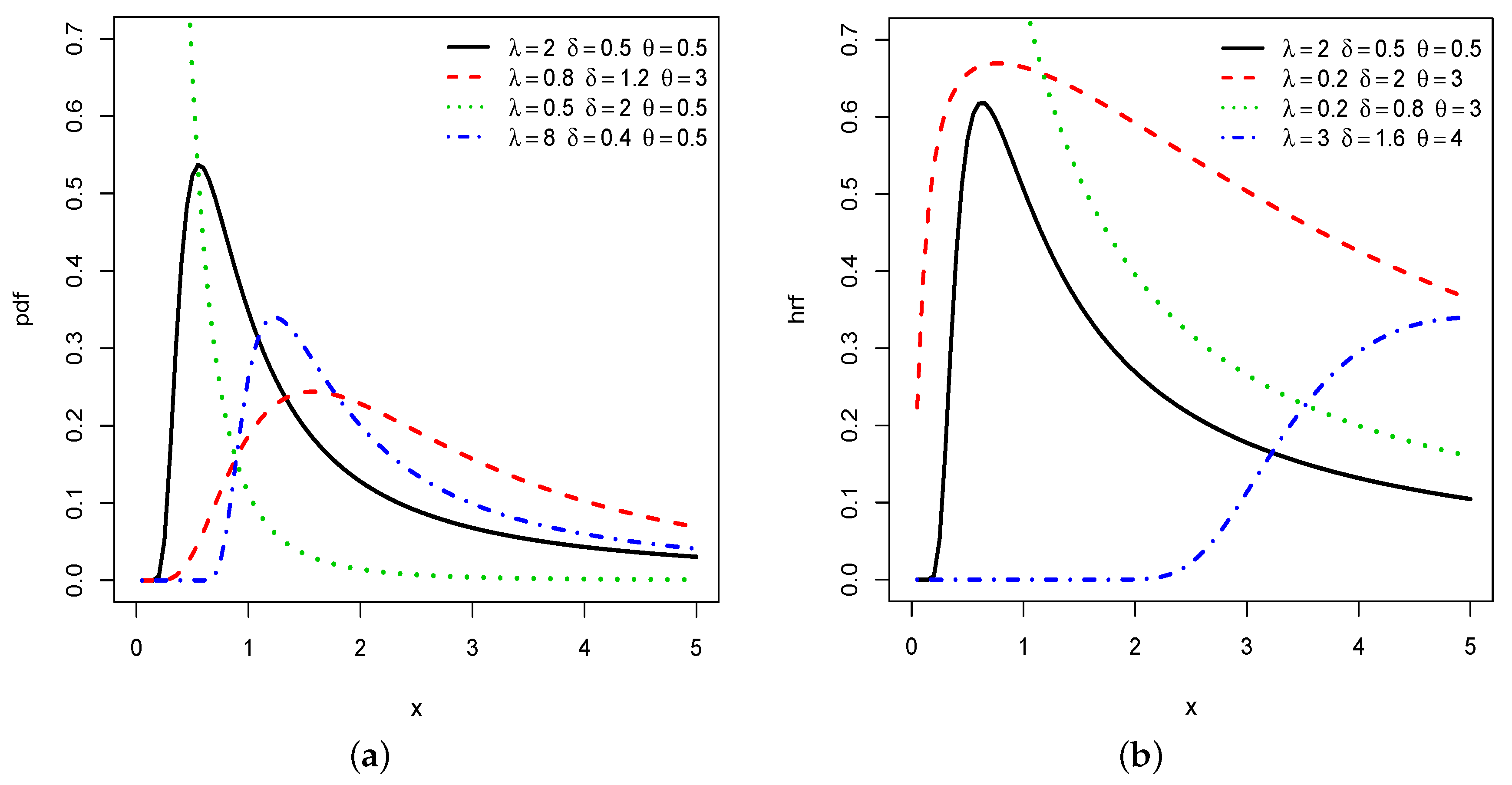
We thus observe that the tails have different decay properties; the right tail has a polynomial decay, whereas the left tail is of exponential decay. The parameter mainly impacts the case . Figure 1 displays plots for the BCG-HC pdfs and hrfs for selected values of , and .
We see various kinds of shapes with different levels of bell shaped and right-skewed. In some cases, a light left tail can be observed. Several tests show that the parameter mainly impacts on the peak of the pdf. These combined features are welcome to construct flexible models for a wide variety of lifetime data.
Now, let us notice that the qf of the half-Cauchy distribution with parameter is given by
The following result in distribution holds. Let Y be a rv with the gamma distribution with parameters 1 and . Then, the rv follows the BCG-HC distribution.
Moreover, based on (5), the BCG-HC qf is obtained as
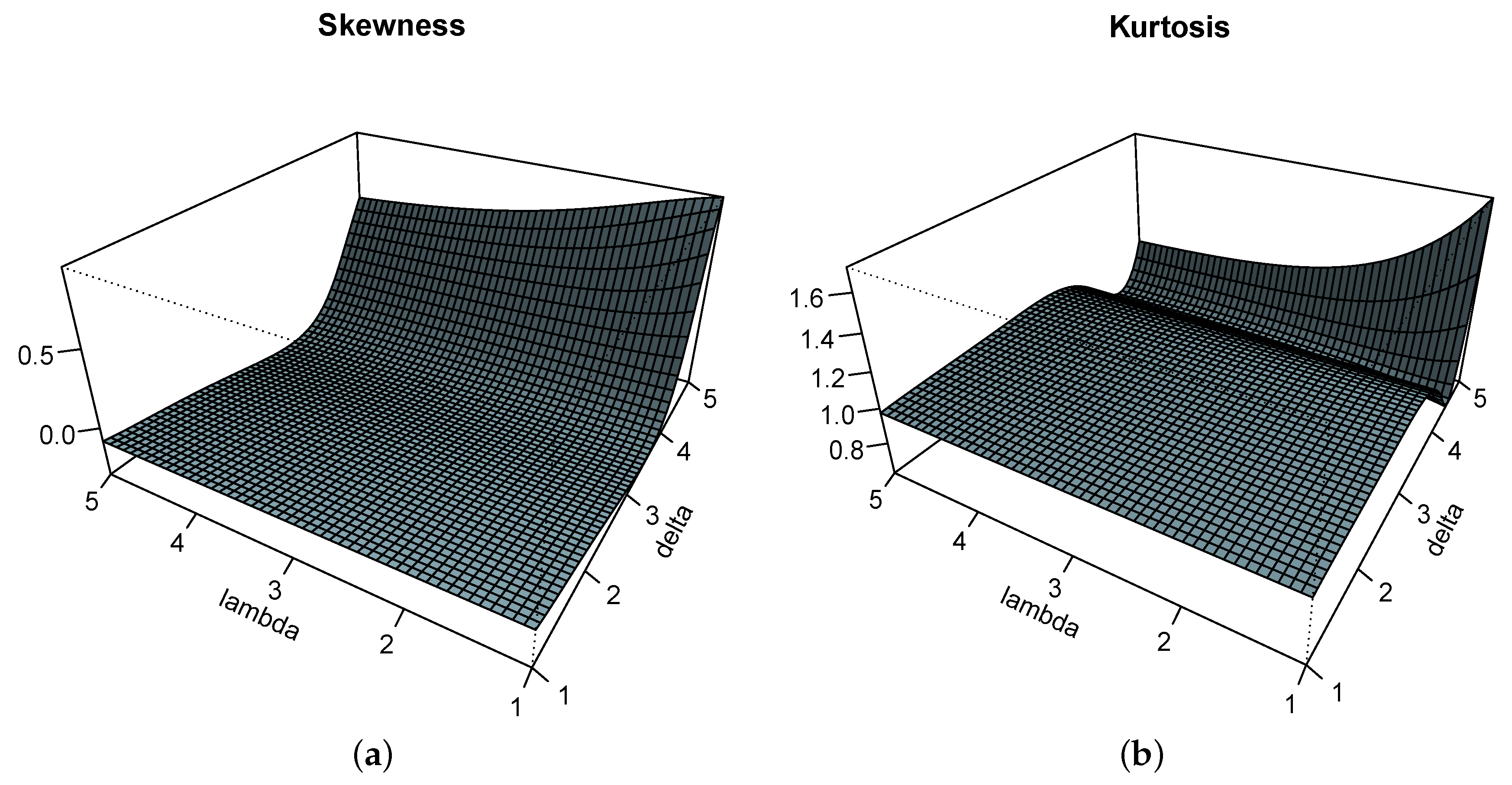
From this qf, we can express the Galton skewness S defined by (6) and the Moors kurtosis K defined by (7). Figure 2 presents the graphics of these two measures for , and .
We observe that S increases when increases, with a various magnitude according to . Varying shapes are observed for K, indicating a non-monotonicity for this measure.
It should be noted that a rv X following the BCG-HC distribution does not have moments of all orders. More precisely, the r-th moment exists if and only if . Indeed, there is no problem of convergence when and, when , we have
which converges as a Riemann integral if and only if . Under this condition, is given by (10). Therefore, if , the variance exists and, if , the skewness and the kurtosis given by (11) exist. Table 2 provides a numerical evaluation of these quantities for selected values for , and .
This approach can be performed to calculate the incomplete moment with a given value for t, means deviation, mean residual life function, moment generating function, Rényi entropy, moments of the order statistics and maximum likelihood estimates (as performed in Section 5.3 for two practical datasets).
5. Statistical Inference and Data Analysis with the BCG-HC Model
Statistical inference and applications of the BCG-HC model with parameters , and , as defined by the cdf in (18) or the pdf in (19), are explored in this section.
5.1. Maximum Likelihood Method
The MLEs , and of the parameters , and , respectively, can be obtained by solving the nonlinear Equations (15)–(17) with the following partial derivatives:
The corresponding SEs can be obtained by the computation of the corresponding observed Fisher information matrix, as described in Section 3.13. These estimates will be considered in the coming simulation and applications studies.
5.2. Simulation Study
Here, following the method described in Section 3.13 and Section 5.1, we check the numerical performance of the MLEs , and in the estimation of , and , respectively, via a complete simulation study. Root mean square errors (RMSEs), as well as lower bounds (LBs), upper bounds (UBs) and average length (ALs) of the asymptotic confidence intervals are determined. The software Mathematica 9 is used. The algorithm of our simulation study is designed as follows.
- 1000 random samples of size n = 50, 100, 200 and 300 are generated from the BCG-HC distribution.
- Values of the true parameters in order: are taken as Set1: , Set2: , Set3: and Set4: .
- The MLEs, RMSEs, LBs, UBs and ALs for the selected sets of values are calculated, considering the levels and for the asymptotic confidence intervals.
With the existing theoretical results of the MLEs in mind, as expected, we notice that the RMSEs and ALs decrease when n increases.
5.3. Data Analysis
Now, we empirically prove the flexibility of the BCG-HC distribution by the analysis of two practical datasets. The BCG-HC distribution will be compared with the competitive models presented in Table 7. The unknown parameters of the models are estimated by the maximum likelihood method. We compare the fitted distributions by using the following usual criteria: , where denotes the maximized log-likelihood, Akaike information criterion (AIC), Bayesian information criterion (BIC), Cramér-Von Mises (CVM), Anderson-Darling (AD) and Kolmogorov-Smirnov (KS) statistics, with the p-value (PV) of the KS test. These measures typically summarize the discrepancy between the data and the expected values under the considered model. In general, the smaller the values of AIC, BIC, CVM, AD and KS, and the greater the values of PV, the better the fit to the data. The software R is used, with the help of the R package entitled AdequacyModel developed by [36].
The two considered datasets are described below.
- Dataset 1:
- We consider the actual taxes dataset used by [39]. The data consist of actual monthly tax revenue in Egypt from January 2006 to November 2010. An immediate histogram plot shows that the distribution of the data is strongly skewed to the right, which
- Dataset 2:
The descriptive statistics of these two datasets are presented in Table 8.
Firstly, let us analyze Dataset 1. Table 9 lists the MLEs and their corresponding SEs (in parentheses) for the BCG-HC model and other fitted models. For the BCG-HC model, these estimates are computed following the methodology described in Section 3.13 and Section 5.1.
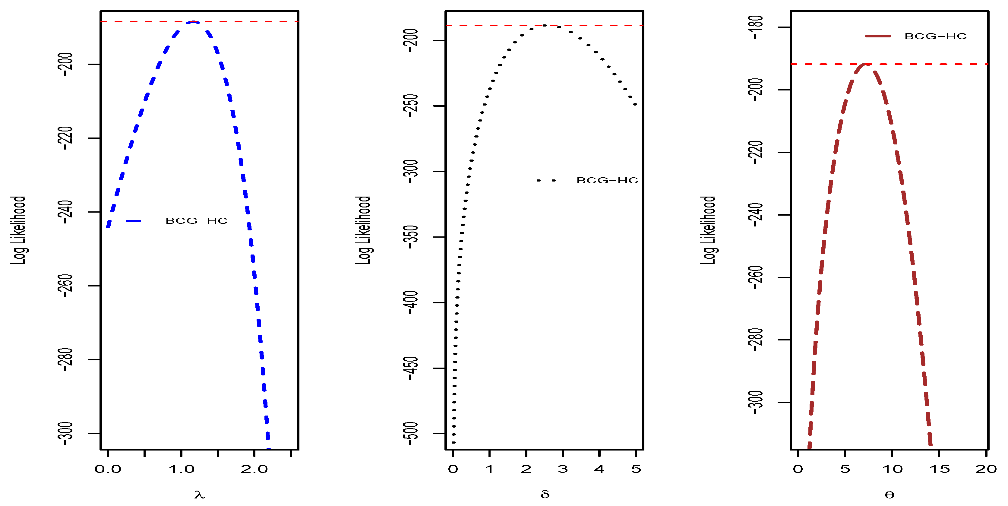
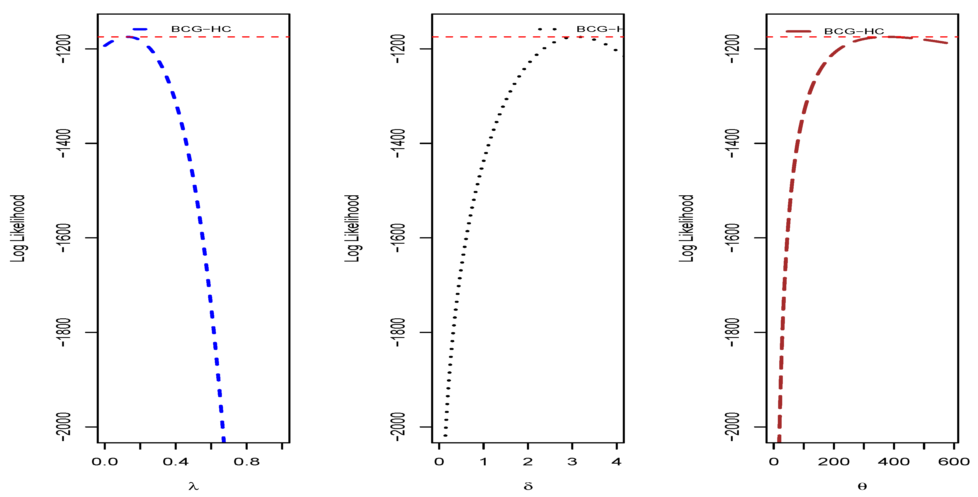
The uniqueness of the obtained MLEs for the BCG-HC model is shown via the profiles plots of the log-likelihood function of , and in Figure 3.
Table 10 indicates the confidence intervals of the parameters of the BCG-HC model for Dataset 1. The levels and are considered.
Table 11 indicates the values of the criteria for the models. From them, we see that the BCG-HC model is the best, having the smallest value of AIC, BIC, CVM, AD and KS, and the largest value of PV.
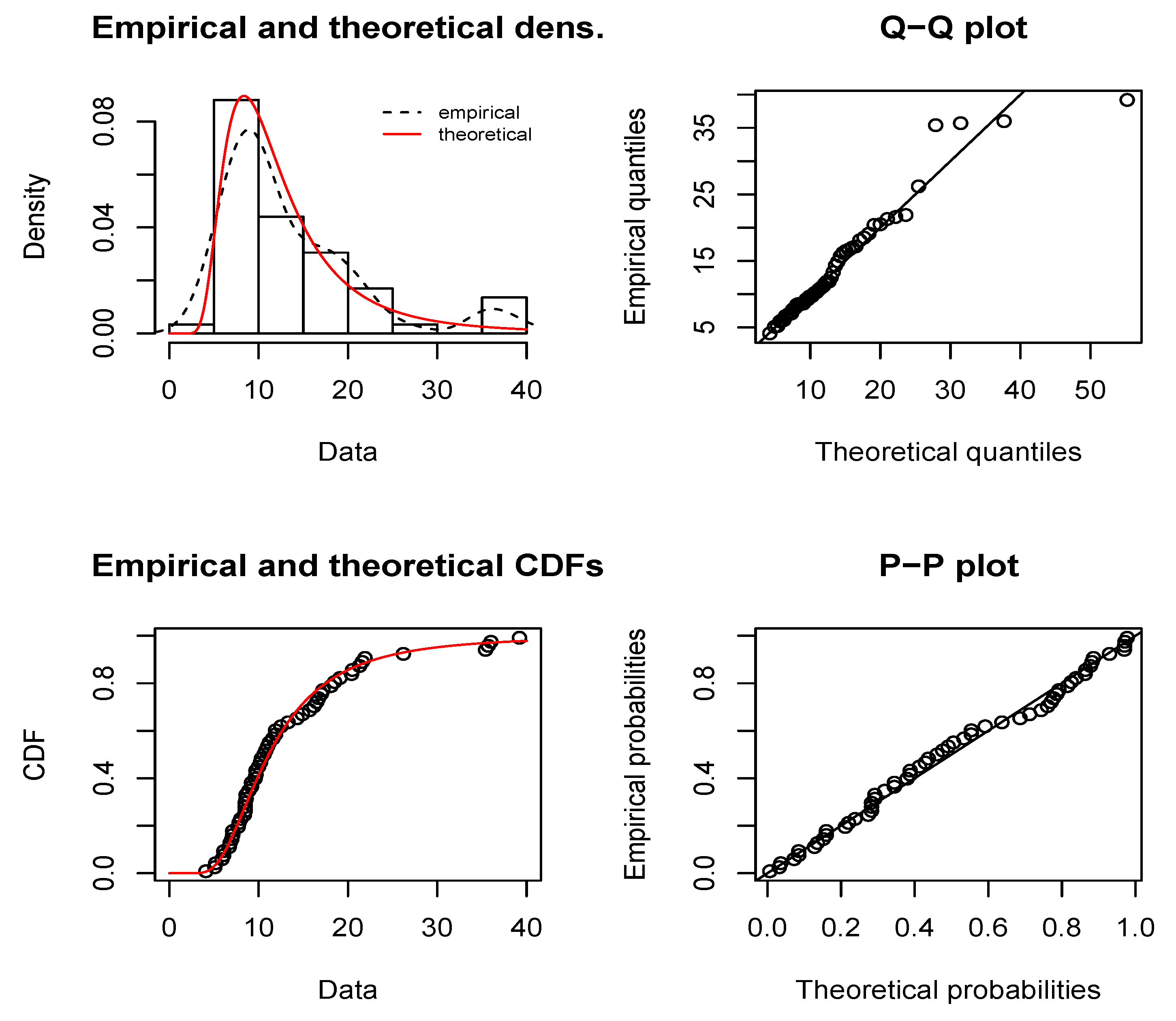
The probability–probability (PP), quantile–quantile (QQ), estimated pdfs (epdfs) and cdfs (ecdfs) plots of the BCG-HC are shown in Figure 4. As anticipated, the best fit is observed for the BCG-HC model.
Now let us proceed to the analysis of Dataset 2 with the same statistical methodology as for Dataset 1. Table 12 lists the MLEs and their corresponding standard errors (in parentheses) for the considered models.
The obtained MLEs for the BCG-HC model are unique. This is shown in Figure 5.
Confidence intervals of the parameters of the BCG-HC model for Dataset 2 are given in Table 13.
Table 14 provides the values of criteria for the BCG-HC model and other fitted models. We thus admit that the BCG-HC model provides a better fit to Dataset 2 than the competitors.
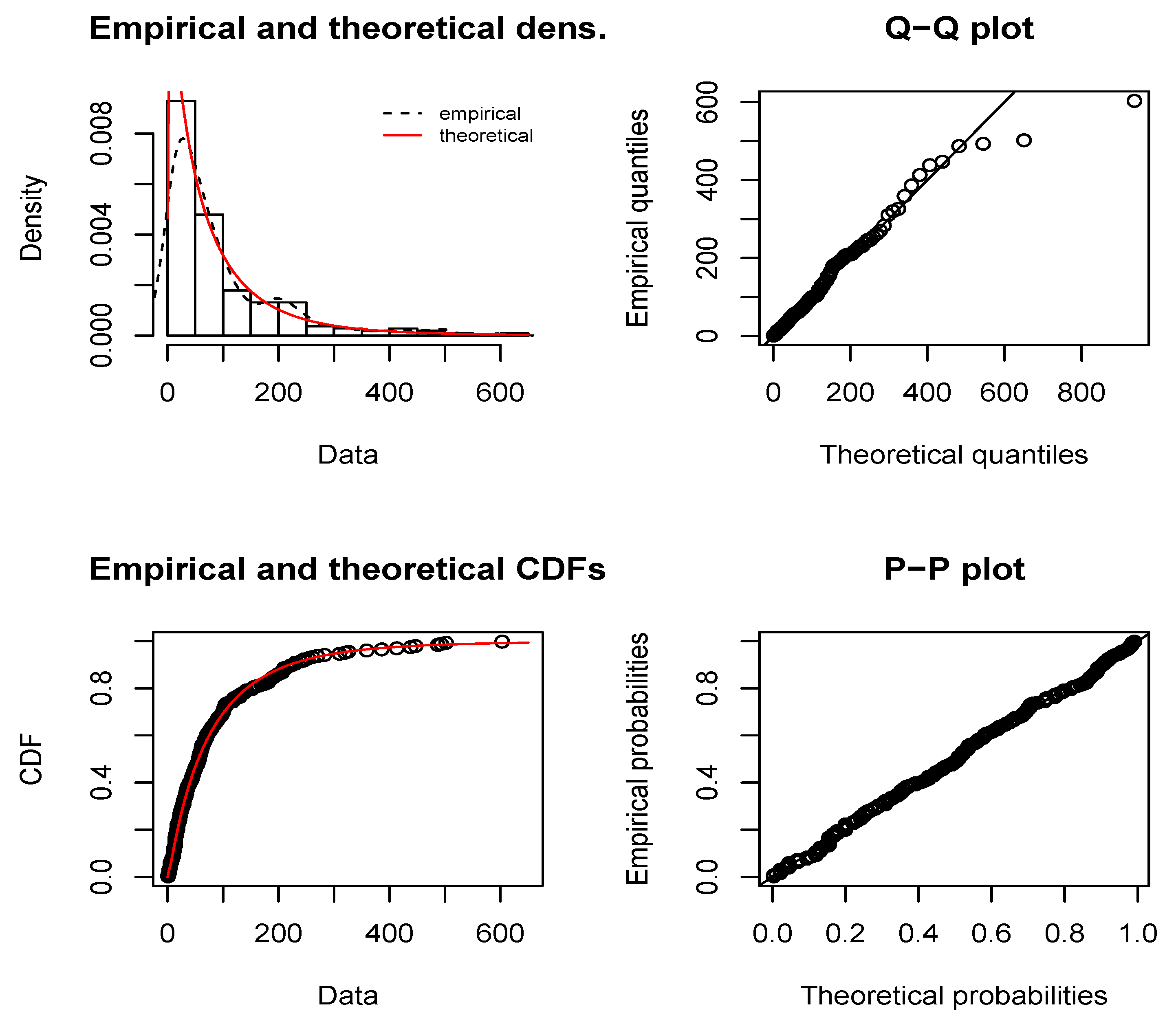
Figure 6 displays the PP, QQ, epdf and ecdf plots of the BCG-HC model. The best fit is observed for the BCG-HC model.
6. Concluding Remarks
In this article, a new family of distributions is presented. It generalizes the RB-G family proposed earlier by [6] through the use of the Box-Cox transformation. The mathematical and practical properties of the BCG-G family are investigated in detail, revealing numerous desirable properties from the theoretical and practical points of view. A member of the BCG-G family extending the half-Cauchy distribution is considered as a statistical model. The parameter estimation is processed and the maximum likelihood estimates are evaluated by simulation study. Two practical datasets are analyzed to illustrate the importance and flexibility of the new model. In fact, it outperforms some generalized half-Cauchy models such as the gamma half-Cauchy, Kumaraswamy half-Cauchy, Marshall Olkin half-Cauchy, exponential half-Cauchy and half-Cauchy models when applied to these datasets. We firmly believe that the proposed family may attract applied statisticians and various scientists from various fields for other modeling purposes.
Author Contributions
A.A.A.-B., I.E., C.C. and F.J. have contributed equally to this work. All authors have read and agreed to the published version of the manuscript.
Funding
This project is supported by Researchers Supporting Project number (RSP-2020/156) King Saud University, Riyadh, Saudi Arabia.
Acknowledgments
The authors thank the two reviewers for their detailed and constructive comments. This work was supported by King Saud University (KSU). The first author, therefore, gratefully acknowledges the KSU for technical and financial support.
Conflicts of Interest
The authors declare no conflict of interest.
References
- Marshall, A.N.; Olkin, I. A new method for adding a parameter to a family of distributions with applications to the exponential and Weibull families. Biometrika 1997, 84, 641–652. [Google Scholar] [CrossRef]
- Gupta, R.C.; Gupta, P.I.; Gupta, R.D. Modeling failure time data by Lehmann alternatives. Comm. Stat. Theory Methods 1998, 27, 887–904. [Google Scholar] [CrossRef]
- Eugene, N.; Lee, C.; Famoye, F. Beta-normal distribution and its applications. Comm. Stat. Theory Methods 2002, 31, 497–512. [Google Scholar] [CrossRef]
- Zografos, K.; Balakrishnan, N. On the families of beta-and gamma-generated generalized distribution and associated inference. Stat. Methodol. 2009, 6, 344–362. [Google Scholar] [CrossRef]
- Cordeiro, G.M.; De Castro, M. A new family of generalized distributions. J. Stat. Comput. Simul. 2011, 81, 883–898. [Google Scholar] [CrossRef]
- Ristić, M.M.; Balakrishnan, N. The gamma-exponentiated exponential distribution. J. Stat. Comput. Simul. 2012, 82, 1191–1206. [Google Scholar] [CrossRef]
- Cordeiro, G.M.; Ortega, E.M.M.; Cunha, D.C. The exponentiated generalized class of distributions. J. Data Sci. 2013, 11, 1–27. [Google Scholar]
- Torabi, H.; Montazeri, N.H. The logistic-uniform distribution and its applications. Commun. Stat. Simul. Comput. 2014, 43, 2551–2569. [Google Scholar] [CrossRef]
- Alzaatreh, A.; Lee, C.; Famoye, F. A new method for generating families of continuous distributions. Metron 2013, 71, 63–79. [Google Scholar] [CrossRef] [Green Version]
- Bourguignon, M.; Silva, R.B.; Cordeiro, G.M. The Weibull-G family of probability distributions. J. Data Sci. 2014, 12, 1253–1268. [Google Scholar]
- Cordeiro, G.M.; Alizadeh, M.; Ortega, E.M.M. The exponentiated half-logistic family of distributions: Properties and applications. J. Probab. Stat. 2014, 2014, 864396. [Google Scholar] [CrossRef]
- Tahir, M.H.; Cordeiro, G.M.; Alizadeh, M.; Mansoor, M.; Zubair, M.; Hamedani, G.G. The odd generalized exponential family of distributions with applications. J. Stat. Distrib. Appl. 2015, 2, 1. [Google Scholar] [CrossRef] [Green Version]
- Jamal, F.; Nasir, M.A.; Tahir, M.H.; Montazeri, N.H. The odd Burr-III family of distributions. J. Stat. Appl. Probab. 2017, 6, 105–122. [Google Scholar] [CrossRef]
- Chesneau, C.; Bakouch, H.S.; Hussain, T. A new class of probability distributions via cosine and sine functions with applications. Commun. Stat. Simul. Comput. 2018, in press. [Google Scholar] [CrossRef]
- Hosseini, B.; Afshari, M.; Alizadeh, M. The Generalized Odd Gamma-G Family of Distributions: Properties and Applications. Austrian J. Stat. 2018, 47, 69–89. [Google Scholar] [CrossRef]
- Bakouch, H.S.; Chesneau, C.; Khan, M.N. The extended odd family of probability distributions with practice to a submodel. Filomat 2020, 33, 3855–3867. [Google Scholar] [CrossRef]
- Jamal, F.; Chesneau, C.; Elgarhy, M. Type II general inverse exponential family of distributions. J. Stat. Manag. Syst. 2020, 23, 617–641. [Google Scholar] [CrossRef] [Green Version]
- Aldahlan, M.A.; Jamal, F.; Chesneau, C.; Elgarhy, M.; Elbatal, I. The truncated Cauchy power family of distributions with inference and applications. Entropy 2020, 22, 346. [Google Scholar] [CrossRef] [Green Version]
- Aldahlan, M.A.; Jamal, F.; Chesneau, C.; Elbatal, I.; Elgarhy, M. Exponentiated power generalized Weibull power series family of distributions: Properties, estimation and applications. PLoS ONE 2020, 15, e0230004. [Google Scholar] [CrossRef] [Green Version]
- Almarashi, A.M.; Elgarhy, M.; Jamal, F.; Chesneau, C. The exponentiated truncated inverse Weibull generated family of distributions with applications. Symmetry 2020, 12, 650. [Google Scholar] [CrossRef] [Green Version]
- Bantan, R.A.R.; Jamal, F.; Chesneau, C.; Elgarhy, M. On a new result on the ratio exponentiated general family of distributions with applications. Mathematics 2020, 8, 598. [Google Scholar] [CrossRef]
- Al-Marzouki, S.; Jamal, F.; Chesneau, C.; Elgarhy, M. Topp-Leone odd Fréchet generated family of distributions with applications to Covid-19 datasets. CMES-Comput. Model. Eng. Sci. 2020, 125, 437–458. [Google Scholar]
- Cordeiro, G.M.; Bourguignon, M. New results on the Ristić–Balakrishnan family of distributions. Comm. Stat. Theory Methods 2016, 45, 6969–6988. [Google Scholar] [CrossRef]
- Oluyede, B.O.; Pu, S.; Makubate, B.; Qiu, Y. The Gamma-Weibull-G Family of Distributions with Applications. Austrian J. Stat. 2018, 47, 45–76. [Google Scholar] [CrossRef] [Green Version]
- Torabi, H.; Montazeri, N.H. The gamma uniform distribution and its applications. Kybernetika 2012, 48, 16–30. [Google Scholar]
- Alzaatreh, A.; Mansoor, M.; Tahir, M.H.; Zubair, M.; Ghazali, S.A. The gamma half-Cauchy distribution: Properties and applications. Hacet. J. Math. Stat. 2016, 45, 1143–1159. [Google Scholar] [CrossRef]
- DiDonato, A.R.; Morris, A.H., Jr. Computation of the incomplete gamma function ratios and their inverse. ACM Trans. Math. Softw. (TOMS) 1986, 12, 377–393. [Google Scholar] [CrossRef]
- Galton, F. Inquiries into Human Faculty and Its Development; Macmillan and Company: London, UK, 1883. [Google Scholar]
- Moors, J.J.A. A quantile alternative for Kurtosis. J. R. Stat. Soc. Ser. D 1988, 37, 25–32. [Google Scholar] [CrossRef] [Green Version]
- Shaked, M.; Shanthikumar, J.G. Stochastic Orders; Wiley: New York, NY, USA, 2007. [Google Scholar]
- Sarabia, J.M. Parametric Lorenz Curves: Models and Applications. In Modeling Income Distribuions and Lorenz Curves; Chotikapanich, D., Ed.; Vol. 5 of Economic Studies in Equality, Social Exclusion and Well-Being; Springer: New York, NY, USA, 2008; Chapter 9; pp. 167–190. [Google Scholar]
- Nanda, A.K.; Singh, H.; Misra, N.; Paul, P. Reliability properties of reversed residual lifetime. Comm. Stat. Theory Methods 2003, 32, 2031–2042. [Google Scholar] [CrossRef]
- Rényi, A. On measures of entropy and information. In Proceedings of the 4th Berkeley Symposium on Mathematical Statistics and Probability, Oakland, CA, USA, 20 June–30 July 1961; Volume 1, pp. 547–561. [Google Scholar]
- Gradshteyn, I.S.; Ryzhik, I.M. Table of Integrals, Series and Products; Academic Press: New York, NY, USA, 2000. [Google Scholar]
- Almarashi, A.M.; Elgarhy, M. A new Muth generated family of distributions with applications. J. Nonlinear Sci. Appl. 2018, 11, 1171–1184. [Google Scholar] [CrossRef] [Green Version]
- Marinho, P.R.D.; Silva, R.B.; Bourguignon, M.; Cordeiro, G.M.; Nadarajah, S. AdequacyModel: An R package for probability distributions and general purpose optimization. PLoS ONE 2019, 14, e0221487. [Google Scholar] [CrossRef] [Green Version]
- Ghosh, I. The Kumaraswamy-half-Cauchy distribution: Properties and applications. J. Stat. Theory Appl. 2014, 13, 122–134. [Google Scholar] [CrossRef] [Green Version]
- Jacob, E.; Jayakumar, K. On half-Cauchy distribution and process. Int. J. Stat. Math. 2012, 3, 77–81. [Google Scholar]
- Mead, M.E. A new generalization of Burr XII distribution. J. Stat. Adv. Theory Appl. 2010, 12, 53–73. [Google Scholar]
- Proschan, F. Theoretical explanation of observed decreasing failure rate. Technometrics 2000, 42, 7–11. [Google Scholar] [CrossRef]
- Dahiya, R.C.; Gurland, J. Goodness of fit tests for the gamma and exponential distributions. Technometrics 1972, 14, 791–801. [Google Scholar] [CrossRef]
- De Andrade, T.A.N.; Zea, L.M.; Gomes-Silva, S.; Cordeiro, G.M. The gamma generalized pareto distribution with applications in survival analysis. Int. J. Stat. Prob. 2017, 6, 141–156. [Google Scholar] [CrossRef] [Green Version]
- Gupta, R.D.; Kundu, D. Exponentiated Exponential Family: An Alternative to Gamma and Weibull Distributions. Biom. J. 2001, 43, 117–130. [Google Scholar] [CrossRef]
- Kus, C. A new lifetime distribution. Comput. Stat. Data Anal. 2007, 51, 4497–4509. [Google Scholar] [CrossRef]
Figure 1.
Plots of some Box-Cox gamma-half-Cauchy (BCG-HC) (a) pdfs and (b) hrfs.

Figure 2.
Bidimensional plots of (a) the Galton skewness S and (b) the Moors kurtosis K for the BCG-HC distribution with parameters , and .
Figure 2.
Bidimensional plots of (a) the Galton skewness S and (b) the Moors kurtosis K for the BCG-HC distribution with parameters , and .

Figure 3.
Profiles plots of the log-likelihood function of the BCG-HC distribution for Dataset 1.

Figure 4.
Probability–probability (PP), quantile–quantile (QQ), estimated pdfs (epdfs) and cdfs (ecdfs) plots of the BCG-HC distribution for Dataset 1.
Figure 4.
Probability–probability (PP), quantile–quantile (QQ), estimated pdfs (epdfs) and cdfs (ecdfs) plots of the BCG-HC distribution for Dataset 1.

Figure 5.
Profiles plots of the log-likelihood function of the BCG-HC distribution for Dataset 2.

Figure 6.
PP, QQ, epdf and ecdf plots of the BCG-HC distribution for Dataset 2.


Table 1.
Some representatives of the Box-Cox gamma-G (BCG-G) family.
| Baseline Distribution | Support | New Cdf | Parameters |
|---|---|---|---|
| Uniform | |||
| Benford | |||
| Exponential | |||
| Weibull | |||
| Pareto | |||
| Fréchet | |||
| Burr XII | |||
| Gamma | |||
| half-Cauchy | |||
| Logistic | |||
| Normal | |||
| Gumbel | |||
| Cauchy |
Table 2.
Mean, variance, skewness and kurtosis for BCG-HC distribution for the following selected parameters values in order : (i): , (ii): , (iii): , (iv): , (v): and (vi): .
Table 2.
Mean, variance, skewness and kurtosis for BCG-HC distribution for the following selected parameters values in order : (i): , (ii): , (iii): , (iv): , (v): and (vi): .
| (i) | (ii) | (iii) | (iv) | (v) | (vi) | |
|---|---|---|---|---|---|---|
| 2.8163 | 41.7295 | 20.1226 | 61.23518 | 31.71016 | 9.656562 | |
| 0.2271 | 834.1558 | 137.7351 | 10090.58 | 5974.927 | 1.632379 | |
| 1.6795 | −0.2009 | 0.02808 | 2.254328 | 3.550561 | 1.299637 | |
| 7.8262 | −1.04022 | −1.8966 | 4.808801 | 13.24243 | 4.022025 |
Table 3.
Maximum likelihood estimates (MLEs), root mean square errors (RMSEs), lower bounds (LBs), upper bounds (UBs) and average length (ALs) of the BCG-HC model for the set of parameters Set1: .
Table 3.
Maximum likelihood estimates (MLEs), root mean square errors (RMSEs), lower bounds (LBs), upper bounds (UBs) and average length (ALs) of the BCG-HC model for the set of parameters Set1: .
| n | MLE | RMSE | 90%LB | 90%UB | 90%AL | 95%LB | 95%UB | 95%AL |
|---|---|---|---|---|---|---|---|---|
| 50 | 0.6156 | 0.0984 | 0.3249 | 0.9063 | 0.5814 | 0.2692 | 0.9620 | 0.6927 |
| 0.6498 | 0.1671 | −0.0400 | 1.3397 | 1.3798 | −0.1722 | 1.4718 | 1.6440 | |
| 0.5573 | 0.0358 | 0.3642 | 0.7503 | 0.3860 | 0.3273 | 0.7872 | 0.4600 | |
| 100 | 0.5694 | 0.0630 | 0.3679 | 0.6709 | 0.3030 | 0.3389 | 0.6999 | 0.3611 |
| 0.5334 | 0.0808 | 0.1659 | 0.9009 | 0.7350 | 0.0955 | 0.9713 | 0.8758 | |
| 0.4662 | 0.0031 | 0.4047 | 0.5878 | 0.1831 | 0.3871 | 0.6053 | 0.2182 | |
| 200 | 0.5340 | 0.0140 | 0.4231 | 0.7049 | 0.2817 | 0.3962 | 0.7319 | 0.3357 |
| 0.5218 | 0.0617 | 0.2559 | 0.9877 | 0.7318 | 0.1858 | 1.0577 | 0.8719 | |
| 0.4845 | 0.0016 | 0.4183 | 0.5707 | 0.1525 | 0.4037 | 0.5853 | 0.1816 | |
| 300 | 0.4807 | 0.0011 | 0.4209 | 0.5406 | 0.1198 | 0.4094 | 0.5521 | 0.1427 |
| 0.4928 | 0.0080 | 0.3148 | 0.6108 | 0.2960 | 0.2864 | 0.6391 | 0.3527 | |
| 0.5016 | 0.0006 | 0.4588 | 0.5444 | 0.0856 | 0.4506 | 0.5526 | 0.1020 |
Table 4.
MLEs, RMSEs, LBs, UBs and ALs of the BCG-HC model for the set of parameters Set2: .
| n | MLE | RMSE | 90%LB | 90%UB | 90%AL | 95%LB | 95%UB | 95%AL |
|---|---|---|---|---|---|---|---|---|
| 50 | 0.9775 | 0.0968 | 0.4213 | 1.5737 | 1.1524 | 0.3110 | 1.6841 | 1.3731 |
| 1.3986 | 0.8164 | −0.1130 | 2.9102 | 3.0232 | −0.4024 | 3.1996 | 3.6021 | |
| 0.5138 | 0.0085 | 0.3844 | 0.6431 | 0.2586 | 0.3597 | 0.6678 | 0.3082 | |
| 100 | 1.0351 | 0.0874 | 0.5965 | 1.4736 | 0.8771 | 0.5126 | 1.5576 | 1.0450 |
| 1.6758 | 0.7029 | 0.3906 | 2.9609 | 2.5702 | 0.1446 | 3.2070 | 3.0624 | |
| 0.5118 | 0.0062 | 0.4223 | 0.6014 | 0.1791 | 0.4051 | 0.6185 | 0.2134 | |
| 200 | 1.0208 | 0.0202 | 0.6646 | 1.3370 | 0.6723 | 0.6003 | 1.4013 | 0.8010 |
| 1.5861 | 0.3644 | 0.5824 | 2.5899 | 2.0075 | 0.3902 | 2.7821 | 2.3919 | |
| 0.5086 | 0.0026 | 0.4366 | 0.5807 | 0.1440 | 0.4228 | 0.5944 | 0.1716 | |
| 300 | 0.9939 | 0.0062 | 0.7830 | 1.1049 | 0.3220 | 0.7521 | 1.1358 | 0.3836 |
| 1.4140 | 0.0303 | 0.9560 | 1.8719 | 0.9159 | 0.8684 | 1.9596 | 1.0913 | |
| 0.5011 | 0.0007 | 0.4630 | 0.5392 | 0.0763 | 0.4557 | 0.5465 | 0.0909 |
Table 5.
MLEs, RMSEs, LBs, UBs and ALs of the BCG-HC model for the set of parameters Set3: .
| n | MLE | RMSE | 90%LB | 90%UB | 90%AL | 95%LB | 95%UB | 95%AL |
|---|---|---|---|---|---|---|---|---|
| 50 | 1.5900 | 1.4331 | −0.0661 | 3.2461 | 3.3122 | −0.3832 | 3.5632 | 3.9464 |
| 1.5106 | 2.4035 | −0.9041 | 4.3253 | 5.2293 | −1.4047 | 4.8260 | 6.2307 | |
| 0.5324 | 0.0032 | 0.3877 | 0.6371 | 0.2494 | 0.3639 | 0.6610 | 0.2971 | |
| 100 | 1.5409 | 0.4954 | 0.6060 | 2.4757 | 1.8697 | 0.4270 | 2.6548 | 2.2278 |
| 1.4475 | 1.4578 | 0.1043 | 3.5907 | 3.4863 | −0.2294 | 3.9245 | 4.1539 | |
| 0.4799 | 0.0029 | 0.3896 | 0.5362 | 0.1467 | 0.3755 | 0.5503 | 0.1747 | |
| 200 | 1.4978 | 0.2224 | 0.8292 | 2.1665 | 1.3372 | 0.7012 | 2.2945 | 1.5933 |
| 1.3364 | 0.9537 | 0.5250 | 3.1478 | 2.6228 | 0.2739 | 3.3990 | 3.1250 | |
| 0.4821 | 0.0018 | 0.4181 | 0.5460 | 0.1279 | 0.4059 | 0.5583 | 0.1524 | |
| 300 | 1.1493 | 0.0129 | 0.9301 | 1.3685 | 0.4383 | 0.8882 | 1.4104 | 0.5223 |
| 1.1775 | 0.0364 | 0.7137 | 1.4413 | 0.7276 | 0.6440 | 1.5110 | 0.8669 | |
| 0.5110 | 0.0006 | 0.4734 | 0.5505 | 0.0771 | 0.4660 | 0.5579 | 0.0919 |
Table 6.
MLEs, RMSEs, LBs, UBs and ALs of the BCG-HC model for the set of parameters Set4: .
| n | MLE | RMSE | 90%LB | 90%UB | 90%AL | 95%LB | 95%UB | 95%AL |
|---|---|---|---|---|---|---|---|---|
| 50 | 1.0456 | 0.7670 | −0.0091 | 2.1004 | 2.1095 | −0.2111 | 2.3023 | 2.5134 |
| 1.1550 | 2.5041 | −0.9199 | 3.2298 | 4.1497 | −1.3172 | 3.6271 | 4.94429 | |
| 0.5148 | 0.0079 | 0.3791 | 0.6505 | 0.2714 | 0.3531 | 0.6765 | 0.323346 | |
| 100 | 0.9334 | 0.1587 | 0.5304 | 1.3365 | 0.8061 | 0.4532 | 1.4136 | 0.960408 |
| 1.0780 | 1.6735 | 0.2184 | 2.3376 | 2.1192 | 0.0155 | 2.5405 | 2.52499 | |
| 0.4956 | 0.0032 | 0.4087 | 0.5826 | 0.1739 | 0.3920 | 0.5992 | 0.207212 | |
| 200 | 0.7876 | 0.0116 | 0.5544 | 1.0208 | 0.4664 | 0.5098 | 1.0654 | 0.555658 |
| 0.8221 | 0.0758 | 0.3170 | 1.3273 | 1.0103 | 0.2202 | 1.4240 | 1.20375 | |
| 0.4964 | 0.0009 | 0.4240 | 0.5687 | 0.1447 | 0.4102 | 0.5826 | 0.172388 | |
| 300 | 0.8105 | 0.0051 | 0.6859 | 0.9432 | 0.2573 | 0.6612 | 0.9678 | 0.306609 |
| 0.8141 | 0.0359 | 0.5928 | 1.1354 | 0.5426 | 0.5408 | 1.1874 | 0.646517 | |
| 0.4979 | 0.0007 | 0.4507 | 0.5251 | 0.0745 | 0.4435 | 0.5323 | 0.088727 |
Table 7.
Coherent competitive models of the BCG-HC distribution.
| Model | Parameters | Cdf | Reference |
|---|---|---|---|
| gamma half-Cauchy (GHC) | [35] | ||
| gamma-exponentiated exponential (GEE) | [6] | ||
| Kumaraswamy half-Cauchy (KHC) | [37] | ||
| Marshall Olkin half-Cauchy (MHC) | [38] | ||
| exponential half-Cauchy (EHC) | [2] | ||
| half-Cauchy (HC) | (Standard) |
Table 8.
Descriptive statistics for Datasets 1 and 2.
| Mean | Median | Variance | Skewness | Kurtosis | |
|---|---|---|---|---|---|
| Dataset 1 | 13.4900 | 10.6000 | 64.8025 | 1.5700 | 2.0800 |
| Dataset 2 | 93.1400 | 57.0000 | 11397.7 | 2.1000 | 4.8500 |
Table 9.
MLEs and standard errors (SEs) (in parentheses) for Dataset 1.
| Model | Estimates | ||
|---|---|---|---|
| BCG-HC | 1.1642 | 2.5801 | 19.4444 |
| () | (0.5017) | (1.1276) | (2.5591) |
| GHC | 17.7164 | 0.1176 | 2.3306 |
| () | (19.2298) | (0.0576) | (3.1104) |
| GEE | 0.2457 | 37.5865 | 0.5408 |
| () | (0.1011) | (4.6796) | (0.2810) |
| KHC | 20.8633 | 4.9716 | 1.6795 |
| () | (3.2415) | (1.2284) | (2.9067) |
| MHC | 1.0729 | 10.9676 | – |
| () | (0.5804) | (4.4320) | – |
| EHC | 5.6949 | 2.6629 | – |
| () | (3.5708) | (1.5689) | – |
| HC | 11.52048 | – | – |
| () | (1.6603) | – | – |
Table 10.
Asymptotic confidence intervals of the parameters of the BCG-HC model for Dataset 1.
| CI | |||
|---|---|---|---|
| [0.1808, 1.8144] | [0.3700, 4.7901] | [14.4285, 24.4602] | |
| [0, 2.4585] | [0, 5.4893] | [12.8419, 26.0468] |
Table 11.
Criteria values for Dataset 1.
| Model | AIC | BIC | CVM | AD | KS | PV | |
|---|---|---|---|---|---|---|---|
| BCG-HC | 188.3004 | 382.0049 | 388.2375 | 0.0465 | 0.2762 | 0.0660 | 0.9589 |
| GHC | 188.5255 | 383.0510 | 389.2836 | 0.0597 | 0.3441 | 0.0708 | 0.9282 |
| GEE | 197.4691 | 400.9382 | 407.1708 | 0.1826 | 1.1285 | 0.1602 | 0.0966 |
| KHC | 188.7694 | 383.5388 | 389.7714 | 0.0683 | 0.3903 | 0.0767 | 0.8781 |
| MHC | 219.7464 | 443.4928 | 447.6478 | 0.1057 | 0.6053 | 0.2483 | 0.0013 |
| EHC | 209.5714 | 423.1428 | 427.2979 | 0.0498 | 0.2919 | 0.2817 | 0.0001 |
| HC | 219.7548 | 441.5097 | 443.5872 | 0.1071 | 0.6133 | 0.2504 | 0.0012 |
Table 12.
MLEs and SEs (in parentheses) for Dataset 2.
| Model | Estimates | ||
|---|---|---|---|
| BCG-HC | 0.1291 | 3.1037 | 375.5790 |
| () | (0.0277) | (0.7969) | (2.5457) |
| GHC | 46.6670 | 0.1919 | 0.0100 |
| () | (7.0641) | (0.0218) | (0.0051) |
| GEE | 0.0026 | 5.0801 | 4.7598 |
| () | (0.0025) | (1.4180) | (0.2454) |
| KHC | 0.9911 | 2.234 | 132.2408 |
| () | (0.1110) | (0.7374) | (3.7441) |
| MHC | 0.4511 | 100.3208 | – |
| () | (0.3240) | (5.1647) | – |
| EHC | 1.1920 | 43.1570 | – |
| () | (0.1658) | (8.0007) | – |
| HC | 52.8000 | – | – |
| () | (4.9808) | – | – |
Table 13.
Asymptotic confidence intervals of the parameters of the BCG-HC model for Dataset 2.
| CI | |||
|---|---|---|---|
| [0.0748, 0.1649] | [1.5417, 4.6656] | [370.5894, 380.5685] | |
| [0.0576, 0.2005] | [1.0476, 5.1597] | [369.0110, 382.1469] |
Table 14.
Criteria values for Dataset 2.
| Model | AIC | BIC | CVM | AD | KS | PV | |
|---|---|---|---|---|---|---|---|
| BCG-HC | 1174.7000 | 2355.4000 | 2365.5000 | 0.0335 | 0.2541 | 0.0380 | 0.9200 |
| GHC | 1185.4000 | 2376.7000 | 2386.8000 | 0.2197 | 1.5109 | 0.0712 | 0.2300 |
| GEE | 1177.4000 | 2360.9000 | 2371.0000 | 0.0847 | 0.5412 | 0.0571 | 0.4900 |
| KHC | 1178.4000 | 2362.8000 | 2372.9000 | 0.0983 | 0.6798 | 0.0501 | 0.6600 |
| MHC | 1185.5000 | 2375.1000 | 2381.8000 | 0.0885 | 0.6624 | 0.0562 | 0.5100 |
| EHC | 1185.6000 | 2375.2000 | 2381.9000 | 0.1764 | 1.1690 | 0.0600 | 0.4300 |
| HC | 1186.4000 | 2374.9000 | 2378.2000 | 0.1303 | 0.9009 | 0.0620 | 0.3900 |
Publisher’s Note: MDPI stays neutral with regard to jurisdictional claims in published maps and institutional affiliations. |
© 2020 by the authors. Licensee MDPI, Basel, Switzerland. This article is an open access article distributed under the terms and conditions of the Creative Commons Attribution (CC BY) license (http://creativecommons.org/licenses/by/4.0/).
Share and Cite
MDPI and ACS Style
Al-Babtain, A.A.; Elbatal, I.; Chesneau, C.; Jamal, F. Box-Cox Gamma-G Family of Distributions: Theory and Applications. Mathematics 2020, 8, 1801. https://0-doi-org.brum.beds.ac.uk/10.3390/math8101801
AMA Style
Al-Babtain AA, Elbatal I, Chesneau C, Jamal F. Box-Cox Gamma-G Family of Distributions: Theory and Applications. Mathematics. 2020; 8(10):1801. https://0-doi-org.brum.beds.ac.uk/10.3390/math8101801
Chicago/Turabian StyleAl-Babtain, Abdulhakim A., Ibrahim Elbatal, Christophe Chesneau, and Farrukh Jamal. 2020. "Box-Cox Gamma-G Family of Distributions: Theory and Applications" Mathematics 8, no. 10: 1801. https://0-doi-org.brum.beds.ac.uk/10.3390/math8101801
Note that from the first issue of 2016, this journal uses article numbers instead of page numbers. See further details here.