Some Intrinsic Properties of Tadmor–Tanner Functions: Related Problems and Possible Applications


Faculty of Mathematics and Informatics, University of Plovdiv Paisii Hilendarski, 24, Tzar Asen Str., 4000 Plovdiv, Bulgaria
Mathematics 2020, 8(11), 1963; https://0-doi-org.brum.beds.ac.uk/10.3390/math8111963
Submission received: 24 September 2020
/
Revised: 11 October 2020
/
Accepted: 12 October 2020
/
Published: 5 November 2020
(This article belongs to the Special Issue Numerical Analysis and Computational Science)
Abstract
:In this paper, we study some properties of an exponentially optimal filter proposed by Tadmor and Tanner. More precisely, we consider the problem for approximating the function of rectangular type by the class of exponential functions about the Hausdorff metric. We prove upper and lower estimates for “saturation”—d (in the case ). New activation and “semi-activation” functions based on are defined. Some related problems are discussed. We also consider modified families of functions with “polynomial variable transfer”. Numerical examples, illustrating our results using CAS MATHEMATICA are given.
1. Introduction
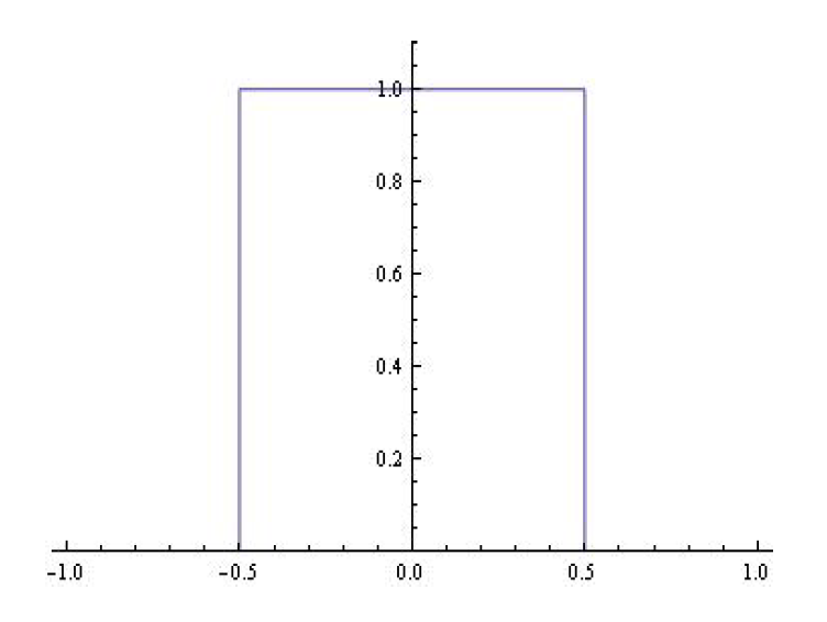
In antenna-feeder techniques, the most often occurred signals are of rectangular type, as shown in Figure 1. In [1,2], the authors construct a new class of accurate filters for processing piecewise smooth spectral data.
Various modifications of this “powerful” class of functions have been proposed and studied by a number of researchers. This study represents a certain interesting problem for approximating the function with the specified class of exponential functions in the Hausdorff sense.
Definition 2
The basic approaches for approximation of functions and point sets of the plane by algebraic and trigonometric polynomials in respect to Hausdorff distance (H–distance) are connected to the work and achievements of Bl. Sendov who established a Bulgarian school in Approximation theory, particularly for developing the theory of Hausdorff approximations.
In this paper we consider some intrinsic properties of function (1). A number of modified adaptive functions have also been proposed that can find application in the field of antenna-feeder analysis. Of course, the specialists working in this direction will assess which of the new models have the right to exist.
2. Main Results
2.1. Some Intrinsic Properties
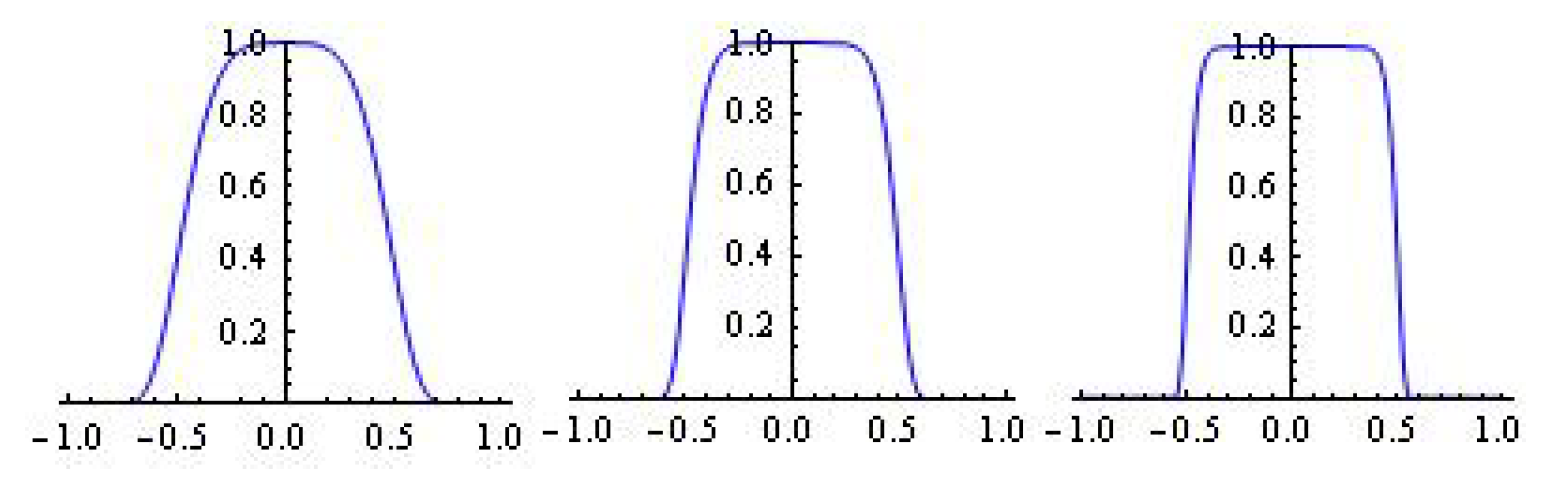
We will consider only the case q–even (see, Figure 2). Let be the value for which —i.e., is the solution of the nonlinear equation:
The Hausdorff distance d between and satisfies the relation:
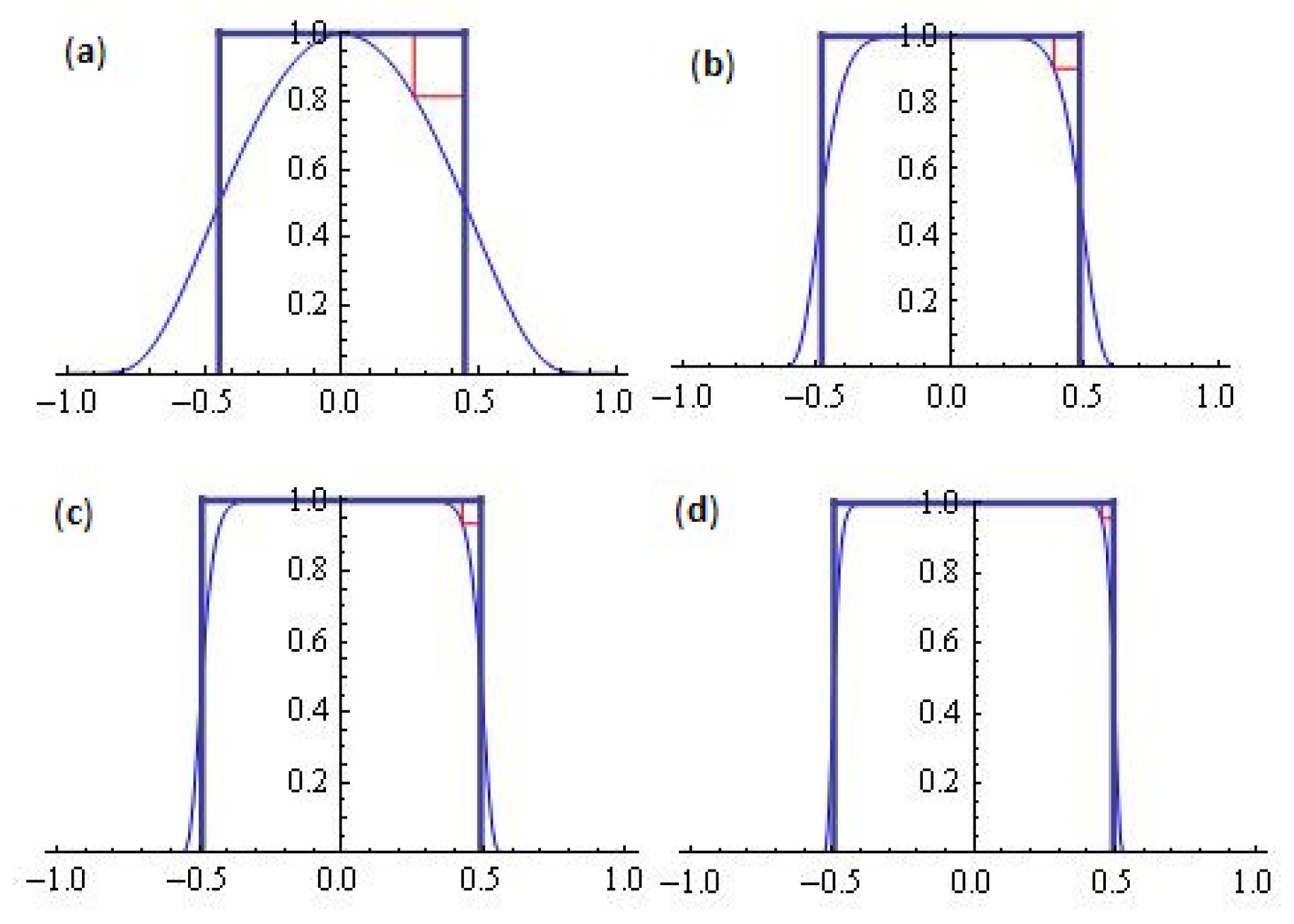
Some computational examples using relations (3) and (4) are depicted on Figure 3. Equations (3) and (4) are nonlinear equations for solving and d. For large values of q, the coefficient grows very rapidly, which severely limits the computational calculations and visualization of the results in any Computer Algebraic Platform. The same remark remains valid when solving the nonlinear Equation (4) for the magnitude of the best Hausdorff approximation—d. This requires obtaining precise two-sided estimates for d. We will sketch the idea, for example, for . Let (see (4))
The following theorem gives upper and lower bounds for d.
Theorem 1.
Let . The “saturation”-d satisfies the following inequalities
where
Proof.
From , we conclude that the function G is strictly monotonically increasing. Consider the function
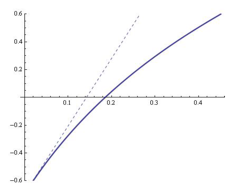
From Taylor expansion, we obtain . Hence, approximates with as (see, Figure 4). In addition, . Further, we have
This completes the proof of the theorem. □
From (5), we see that for , .
The reader may formulate the corresponding approximation problem for arbitrary q following the ideas given in this note, and this will be omitted. Some techniques for obtaining accurate two-sided estimates can be found in [7].
2.2. Some Remarks
The basic problems considered in [8,9,10]) are an approximation of functions and point sets by algebraic and trigonometric polynomials in the Hausdorff metric as well as their applications in the field of antenna-feeder techniques, analysis and the synthesis of antenna patterns and filters, including noise minimization by the suitable approximation of impulse functions.
The application of Fourier analysis for the approximation of impulse and transmitting functions is compared to this, which can be obtained using the elements of the best Hausdorff approximation.
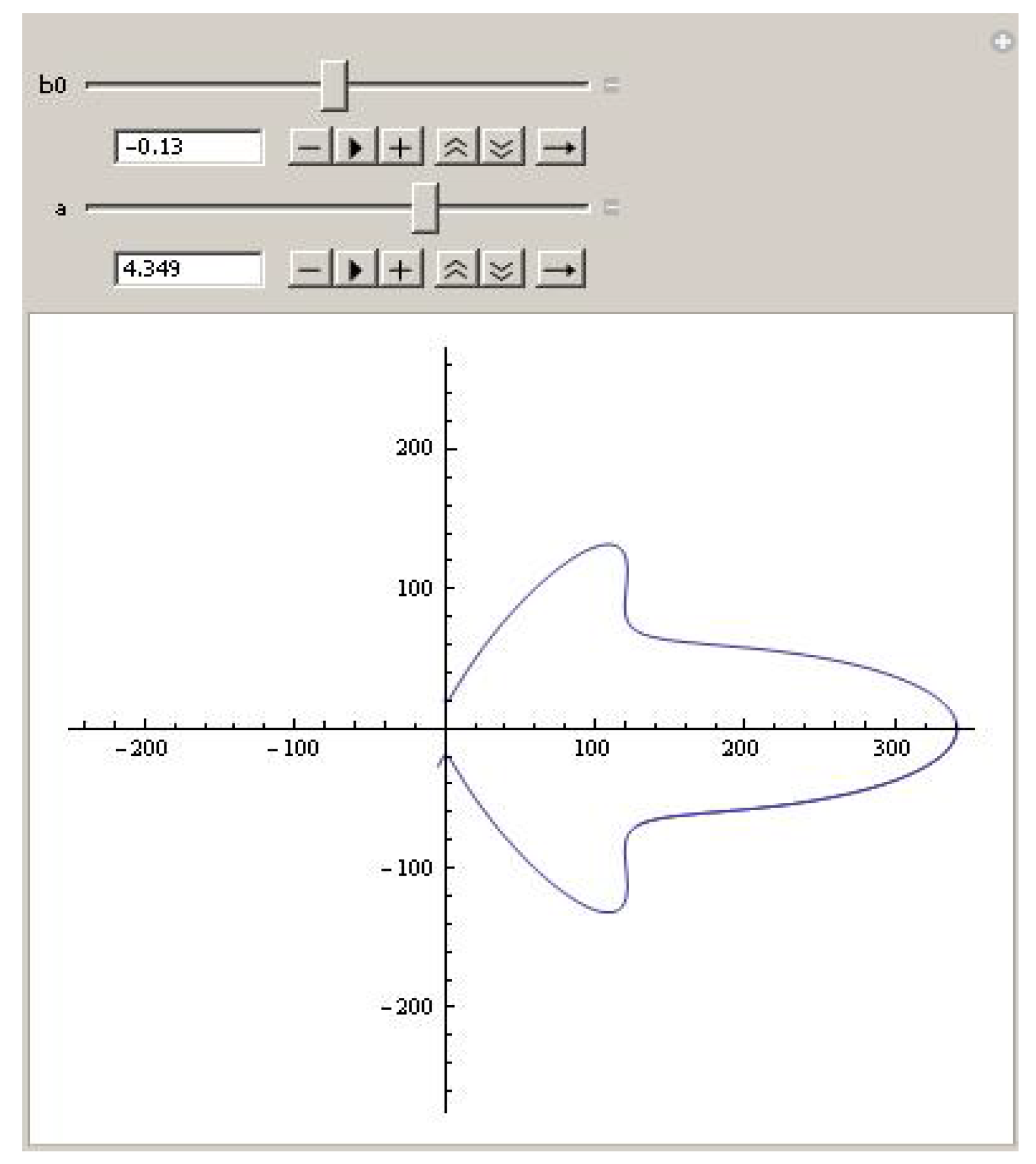
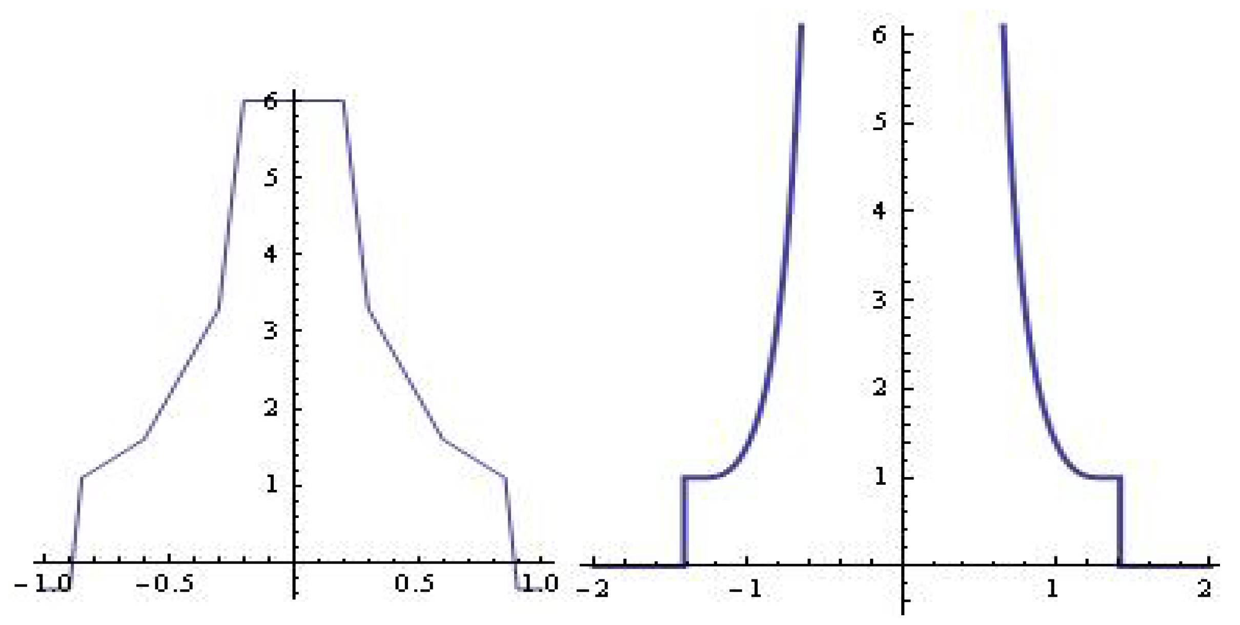
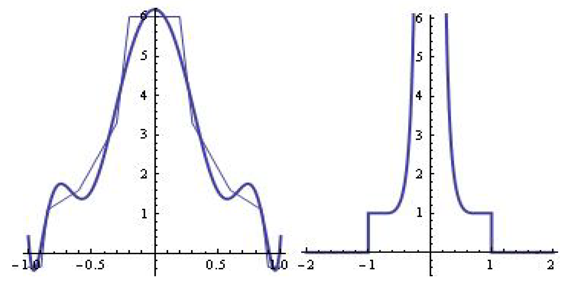
- Modified Families with ”Polynomial Variable Transfer”Following the ideas formally given by us, we consider the following modified families of functions based on with “polynomial variable transfer”:andThe modified families: for and for are depicted in Figure 6.Let , where is azimuthal angle and a is the phase difference.Then, for example, typical radiation patterns with “restrictions” using for(a) ;(b)Numerical examples are presented using CAS MATHEMATICA.
- The New Activation FunctionWe define the following activation function based on (1):In antenna-feeder technique most often occurred signals are of types shown in Figure 9 and Figure 10. For q even, the corresponding approximation using model (9) is shown in Figure 9. For q odd, the corresponding approximation using new activation function is shown in Figure 10.The reader may formulate the corresponding approximation problem following the ideas given in this article, and this will be omitted. The results have important role in the fields of Population Dynamics, Biostatistics, Signal Theory, Reliability Analysis and Life testing experiments. For other results, see [12,13,14,15]. Another application of the Hausdorff metric can be found in [16].
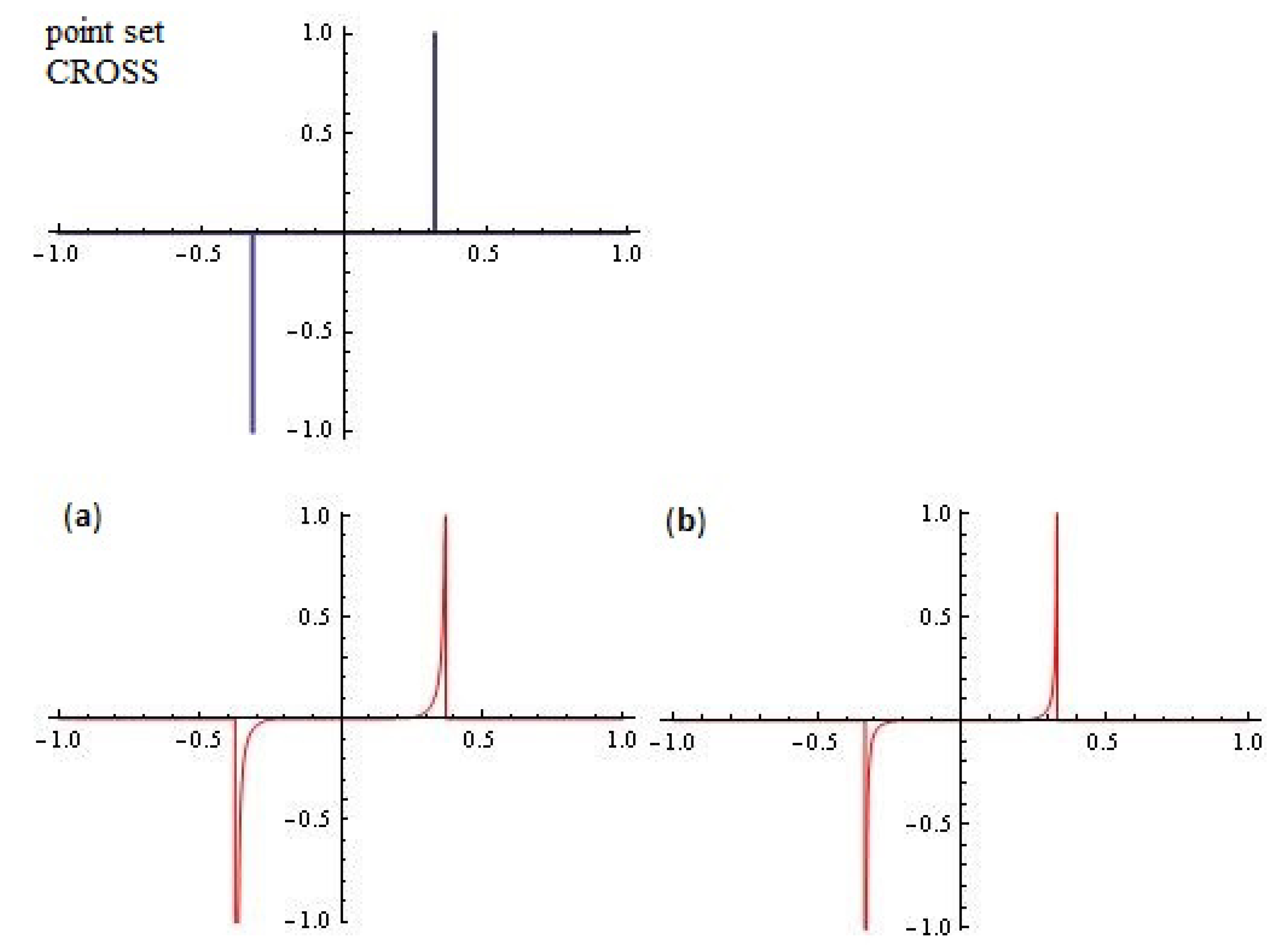
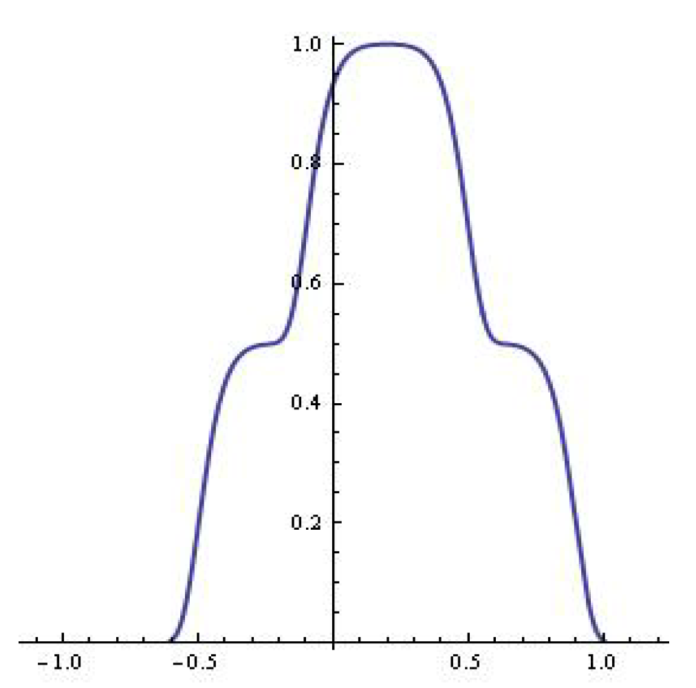
- New ”semi-activation” functionWe define the following “semi-activation” functionThe problem of approximating the “point set” depicted in Figure 11 is also of independent interest (in the limiting case, the “point set CROSS”—see, for instance, [17]).The modified family for :(a) ;(b)is depicted in Figure 11.
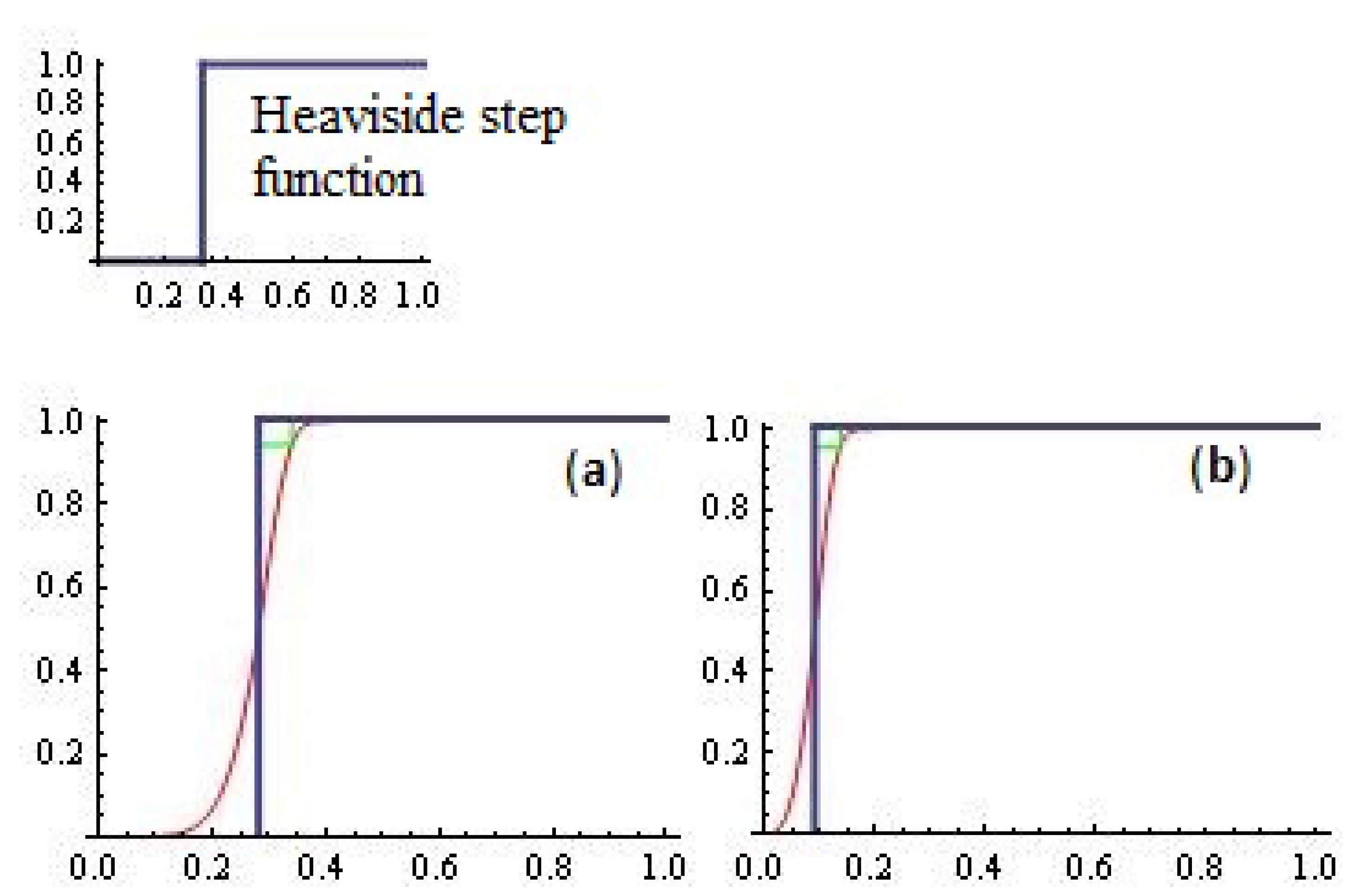
- Another activation functionFormally, we define the following activation functionwhere .The shifted Heaviside step function is defined byObviously, the new function can be used successfully to approximate the Heaviside step function (see Figure 12).Approximation of shifted Heaviside step function by sigmoidal function for:(a) : ; Hausdorff distance ;(b) ; Hausdorff distanceis visualized on Figure 12.The function can be used in the field of population dynamics and biostatistics [7].
- The new functionFormally, we define the following function:where and are polynomials.In some cases, the function can be used for analysis of “rectangular signals”.For example, see Figure 13 for fixedand.Remark 1.is the polynomial of best one–sided Hausdorff distance of the functionby polynomial of degree 10 (see, for example, [4]).Let .Unfortunately, these diagrams cannot always be realized in practice.
- Application to the ”cut-off function”The analysis presented in this article can also be applied to the “cut-off function”, see (1):where and p is even.
- Approximation with restrictionsOften some restrictions must be imposed on the main lobe of the radiation pattern—for example, see Figure 16The polynomialcomputed by Remez’s algorithm from [18] and shown in Figure 17, provides a reliable approximation of the window (Figure 16).We note that the “adaptive function” withbased on function of Tadmor and Tanner (1) is of the form shown in Figure 17.Unfortunately, these diagrams cannot always be realized in practice.Specialists working in these scientific fields have the final word.We will look at another instructive example.A typical diagram function with imposed constraints at the median level is shown in Figure 18.After serious analysis, it turned out that the function by Tadmor and Tanner could be modified in such a way as to obtain the following “differential analogue with step h”:whereandFrom the attached visualization (see Figure 19 and Figure 20) it can be seen that the proposed new modification can be used successfully for the approximation of functions of type .Obviously, higher order differential analogues can be obtained, which we leave to the readers’ attention.
3. Concluding Remarks
The aim of the present research is to define families of “adaptive functions” that could be used in various branches of scientific knowledge, in particular in the approximation of a number of classical impulse signals, point sets in the plane and supplemented graphs of discontinuous functions.
Questions related to the synthesis and analysis of transfer functions, radiation diagrams with algebraic and trigonometric polynomials about Hausdorff distance are elaborated in detail in the monograph in [8].
In this article we consider only some aspects related to the disclosure of intrinsic properties of some of the proposed families of “adaptive functions” in a purely methodological aspect.
Many of the proposed new models could not be used as “feasible models–diagrams” in practice.
Funding
This research received no external funding.
Acknowledgments
This work has been accomplished with the financial support by the Grant No BG05M2OP001-1.001-0003, financed by the Science and Education for Smart Growth Operational Program (2014–2020) and co-financed by the European Union through the European structural and Investment funds.
Conflicts of Interest
The author declares no conflict of interest.
References
- Tadmor, E.; Tanner, J. Adaptive filters for piecewise smooth spectral data. SIMA J. Numer. Alg. 2005, 25, 535–547. [Google Scholar]
- Tanner, J. Optimal filter and mollifier for piecewise smooth spectral data. Math. Comput. 2006, 75, 767–790. [Google Scholar] [CrossRef] [Green Version]
- Hausdorff, F. Set Theory, 2nd ed.; Chelsea Publ.: New York, NY, USA, 1962. [Google Scholar]
- Sendov, B. Hausdorff Approximations; Kluwer: Boston, MA, USA, 1990. [Google Scholar]
- Sendov, B.; Popov, V. The exact asymptotic behavior of the best approximation by algebraic and trigonometric polynomials in the Hausdorff metric. Math. USSR-Sb 1972, 89, 138–147. (In Russian) [Google Scholar] [CrossRef]
- Anguelov, R.; Markov, S.; Sendov, B. On the Normed Linear Space of Hausdorff Continuous Functions. Lecture Notes Comput. Sci. 2006, 3743, 281–288. [Google Scholar]
- Kyurkchiev, N.; Markov, S. On the Hausdorff distance between the Heaviside step function and Verhulst logistic function. J. Math. Chem. 2016, 54, 109–119. [Google Scholar] [CrossRef]
- Kyurkchiev, N.; Andreev, A. Approximation and Antenna and Filter Synthesis: Some Moduli in Programming Environment Mathematica; Lap Lambert Academic Publishing: Saarbrucken, Germany, 2014. [Google Scholar]
- Andreev, A.; Kyurkchiev, N. Approximation of some impulse functions—implementation in programming environment MATHEMATICA. In Proceedings of the 43 Spring Conference of the Union of Bulgarian Mathematicians, Borovetz, Bulgaria, 2–6 April 2014; pp. 111–117. [Google Scholar]
- Golev, A.; Djamiykov, T.; Kyurkchiev, N. Sigmoidal Functions in Antenna-feeder Technique. Int. J. Pure Appl. Math. 2017, 116, 1081–1092. [Google Scholar]
- Gelb, A.; Tanner, J. Robust reprojection methods for the resolution of the Gibbs phenomenon. Appl. Comput. Harmon. Anal. 2006, 20, 3–25. [Google Scholar] [CrossRef]
- Kyurkchiev, N.; Iliev, A.; Rahnev, A. On the Half-Logistic Model with “polynomial variable transfer”. Application to approximate the specific “data CORONA VIRUS”. Int. J. Differ. Equations Appl. 2020, 19, 45–61. [Google Scholar]
- Kyurkchiev, N. Selected Topics in Mathematical Modeling: Some New Trends (Dedicated to Academician Blagovest Sendov (1932–2020)); Lap Lambert Academic Publishing: Saarbrucken, Germany, 2020. [Google Scholar]
- Costarelli, D.; Spigler, R. Constructive Approximation by Superposition of Sigmoidal Functions. Anal. Theory Appl. 2013, 2013 29, 169–196. [Google Scholar]
- Kyurkchiev, N.; Nikolov, G. Comments on some new classes of sigmoidal and activation functions. Applications. Dyn. Syst. Appl. 2019, 28, 789–808. [Google Scholar]
- Peters, J. Foundations of Computer Vision: Computational Geometry, Visual Image Structures and Object Shape Detection; Springer: Cham, Switzerland, 2017. [Google Scholar]
- Kyurkchiev, N.; Markov, S. On the numerical approximation of the “cross” set. Ann. Univ. Sofia Fac. Math. 1974, 66, 19–25. (In Bulgarian) [Google Scholar]
- Tashev, S. Approximation of bounded sets on the plane in Hausdorff metric. CR Acad. Bulg. Sci. 1976, 29, 465–468. (In Russian) [Google Scholar]
- Petrushev, P.; Popov, V. Rational Approximation of Real Functions; Cambridge University Press: Cambridge, UK, 1987. [Google Scholar]
- Ivanov, K.; Totik, V. Fast Decreasing Polynomials. Constr. Approx. 1990, 6, 1–20. [Google Scholar] [CrossRef]
- Kyurkchiev, N.; Andreev, A. Hausdorff approximation of functions different from zero at one point—implementation in programming environment MATHEMATICA. Serdica J. Comput. 2013, 7, 135–142. [Google Scholar]
- Kyurkchiev, N.; Andreev, A. Synthesis of slot aerial grids with Hausdorff–type directive patterns–implementation in programming environment Mathematica. CR Acad. Bulg. Sci. 2013, 66, 1521–1528. [Google Scholar]
- Kyurkchiev, N. Synthesis of Slot Aerial Grids with Hausdorff Type Directive Patterns. Ph.D. Thesis, VMEI, Sofia, Bulgaria, 1979. (In Bulgarian). [Google Scholar]
- Sendov, B.L.; Schinev, H.; Kjurkchiev, N. Hausdorff-synthesis of aerial grids in scanning the directive diagram. Electropromishlenost Prib. 1984, 16, 203–205. (In Bulgarian) [Google Scholar]
- Schinev, H.; Kjurkchiev, N.; Gachev, M. Experimental investigations of slot aerial grids with Hausdorff type directive patterns. Electropromishlenost Prib. 1979, 14, 223–224. (In Bulgarian) [Google Scholar]
- Shinev, H.; Kyurkchiev, N.; Gachev, M.; Markov, S. Application of a class of polynomials of best approximation to linear antenna array synthesis. Izv. Vmei Sofia 1975, 34, 1–6. (In Bulgarian) [Google Scholar]
- Kyurkchiev, N.; Sendov, B.L. Approximation of a class of functions by algebraic polynomials with respect to Hausdorff distance. Ann. Univ. Sofia Fac. Math. 1975, 67, 573–579. (In Bulgarian) [Google Scholar]
- Appostolov, P. General theory, approximation method and design of electrical filters based on Hausdorff polynomials. Mech. Transp. Commun. 2007, 2, 1–8. (In Bulgarian) [Google Scholar]
- Kyurkchiev, N.; Iliev, A.; Rahnev, A. A Look at the New Logistic Models with “Polynomial Variable Transfer”; Lap Lambert Academic Publishing: Saarbrucken, Germany, 2020. [Google Scholar]
- Kyurkchiev, N.; Iliev, A.; Golev, A.; Rahnev, A. Some Non-standard Models in “Debugging and Test Theory” (Part 4); Plovdiv University Press: Plovdiv, Bulgaria, 2020. [Google Scholar]
- Costarelli, D.; Vinti, G. Pointwise and uniform approximation by multivariate neural network operators of the max-product type. Neural Netw. 2016, 81, 81–90. [Google Scholar] [CrossRef]
- Guliyev, N.; Ismailov, V. A single hidden layer feed forward network with only one neuron in the hidden layer san approximate any univariate function. Neural Comput. 2016, 28, 1289–1304. [Google Scholar]
- Iris, C.; Pacino, D.; Ropke, S.; Larsen, A. Integrated berth allocation and quay crane assignment problem: Set partitioning models and computational results. Transp. Res. Part Logist. Transp. Rev. 2015, 81, 75–97. [Google Scholar] [CrossRef] [Green Version]
- Mauri, G.R.; Ribeiro, G.M.; Lorena, L.A.N.; Laporte, G. An adaptive large neighborhood search for the discrete and continuous berth allocation problem. Comput. Oper. Res. 2016, 70, 140–154. [Google Scholar] [CrossRef]
- Kyurkchiev, N. A new class of activation functions. Some related problems and applications. Biomath 2020, 9, 10. [Google Scholar] [CrossRef]
- Kyurkchiev, N.; Iliev, A.; Markov, S. Some Techniques for Recurrence Generating of Activation Functions: Some Modeling and Approximation Aspects; Lap Lambert Academic Publishing: Saarbrucken, Germany, 2017. [Google Scholar]
- Iliev, A.; Kyurkchiev, N.; Markov, S. A Note on the New Activation Function of Gompertz Type. Biomath Commun. 2017, 4, 20. [Google Scholar] [CrossRef] [Green Version]
- Kyurkchiev, N.; Iliev, A.; Rahnev, A. A new class of activation functions based on the correcting amendments of Gompertz-Makeham type. Dyn. Syst. Appl. 2019, 28, 243–257. [Google Scholar] [CrossRef] [Green Version]
- Kyurkchiev, N. Comments on the Yun’s algebraic activation function. Some extensions in the trigonometric case. Dyn. Syst. Appl. 2019, 28, 533–543. [Google Scholar]
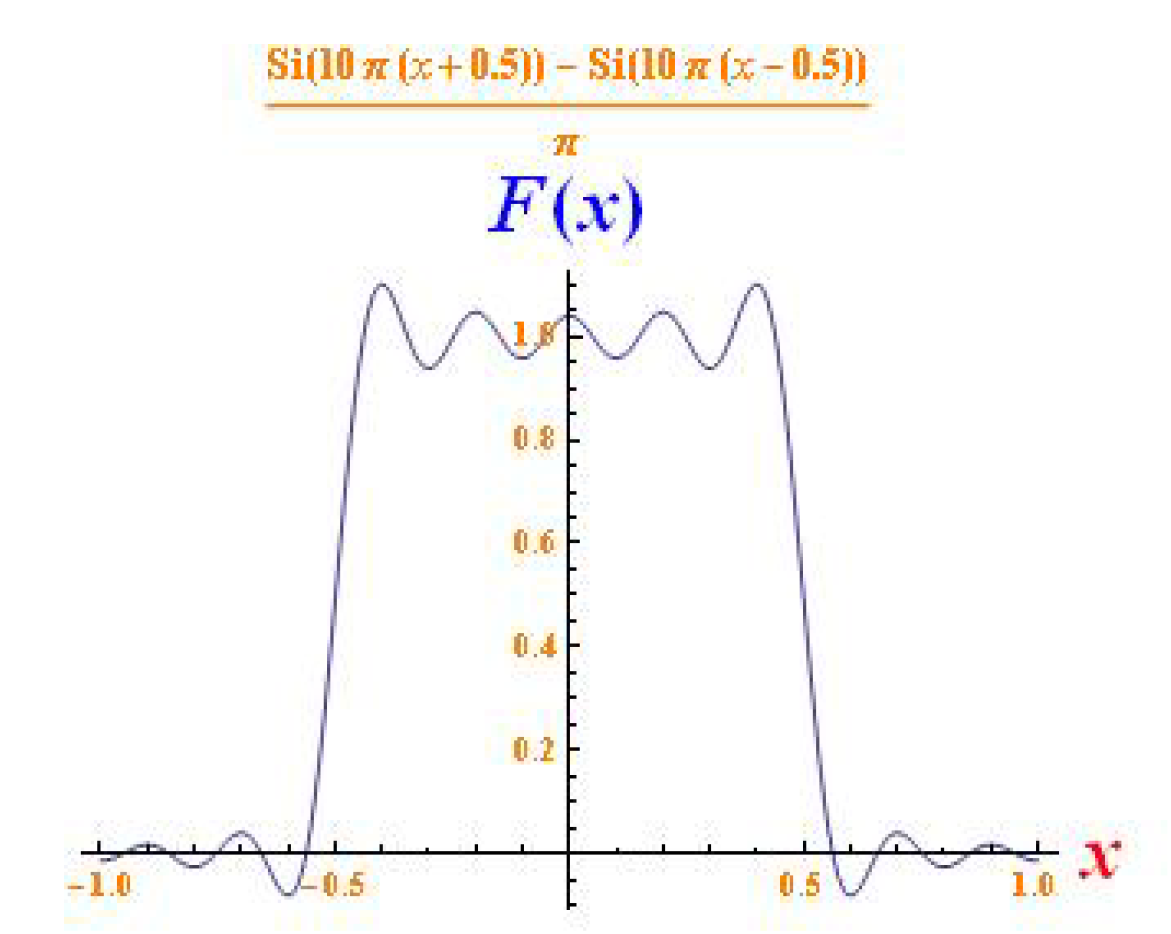
Figure 1.
Signal of rectangular type—.

Figure 2.
The exponentially optimal filter for .

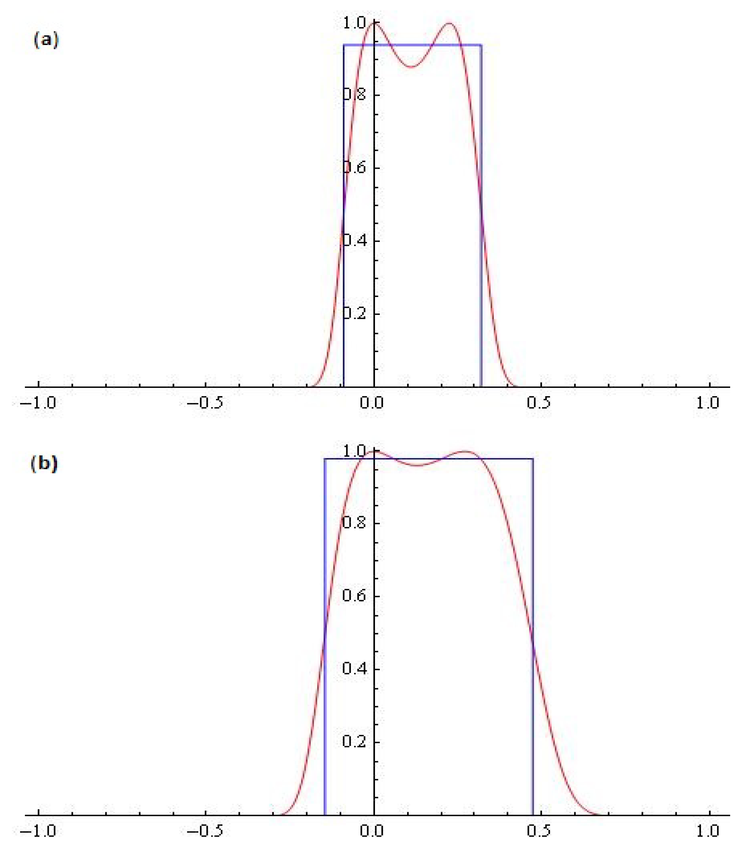
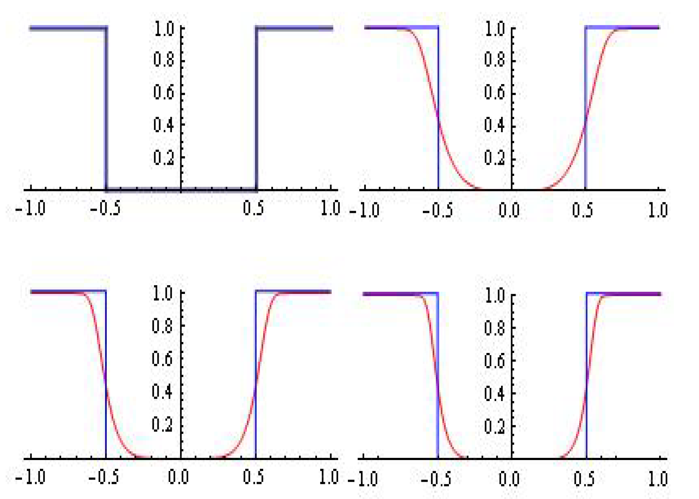
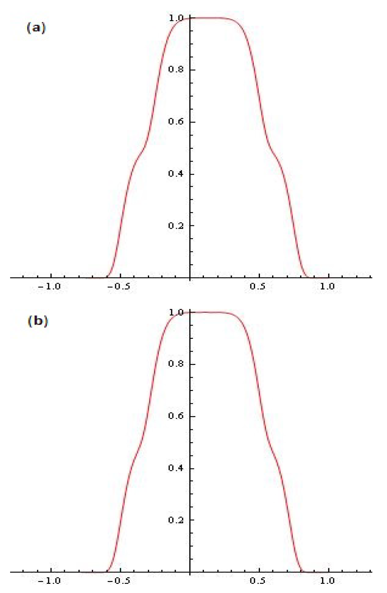
Figure 3.
Approximation of by : (a) ; Hausdorff distance =; (b) ; Hausdorff distance ; (c) ===; Hausdorff distance ; (d) ===; Hausdorff distance .
Figure 3.
Approximation of by : (a) ; Hausdorff distance =; (b) ; Hausdorff distance ; (c) ===; Hausdorff distance ; (d) ===; Hausdorff distance .

Figure 4.
The functions and for .

Figure 5.
A typical application of Fourier transform to analysis of radiation patterns (“Gibbs’ phenomenon”) [8].
Figure 5.
A typical application of Fourier transform to analysis of radiation patterns (“Gibbs’ phenomenon”) [8].

Figure 6.
(a) Modified family for ; (b) Modified family for .

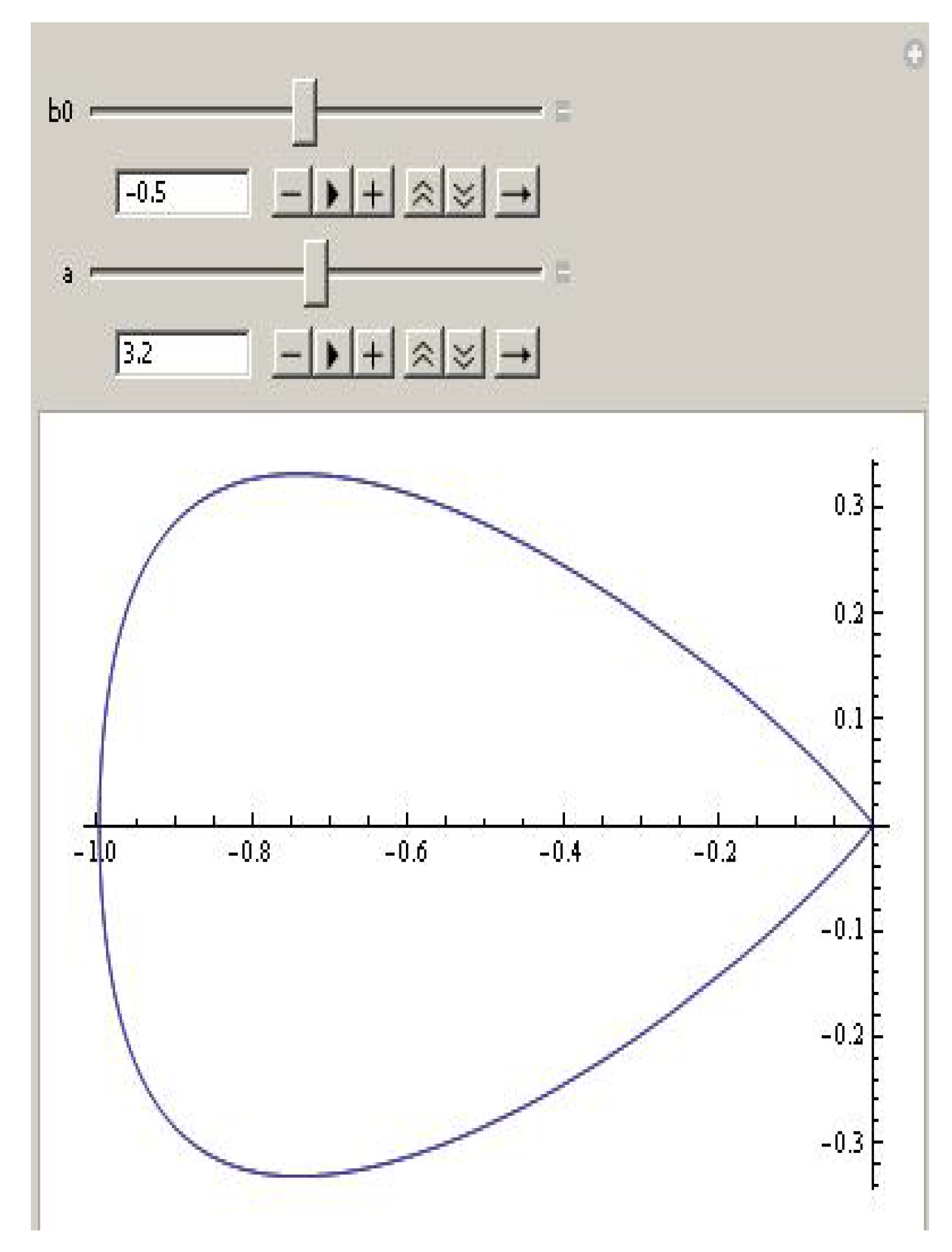
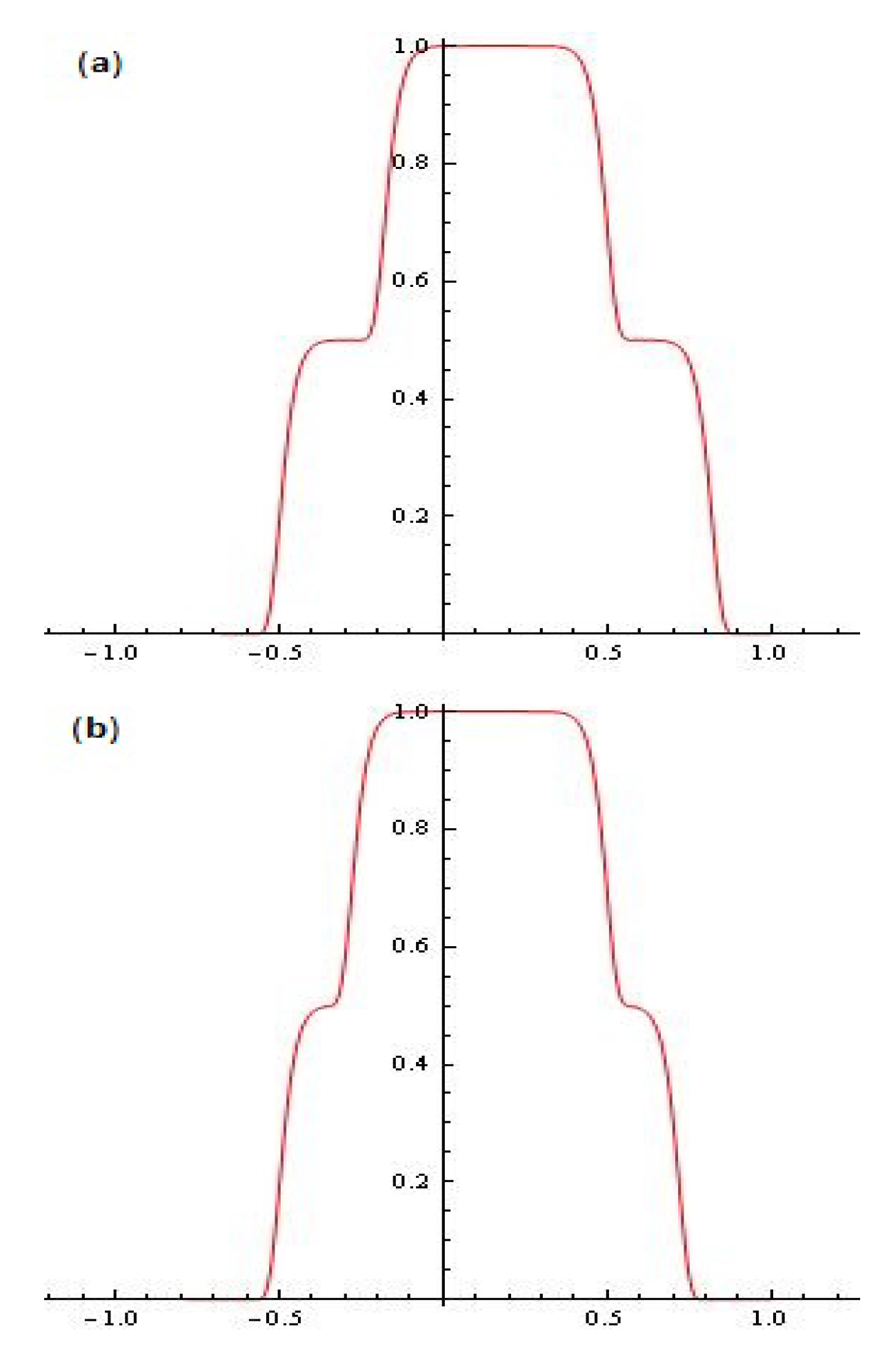
Figure 7.
A typical radiation pattern with “restrictions” using for ====, ====.

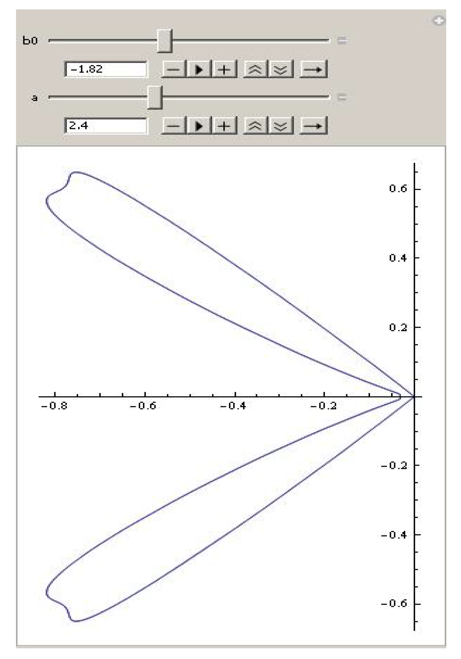
Figure 8.
A typical radiation pattern with “restrictions” using for ==, =.

Figure 9.
Approximation by for .

Figure 10.
Approximation by for .

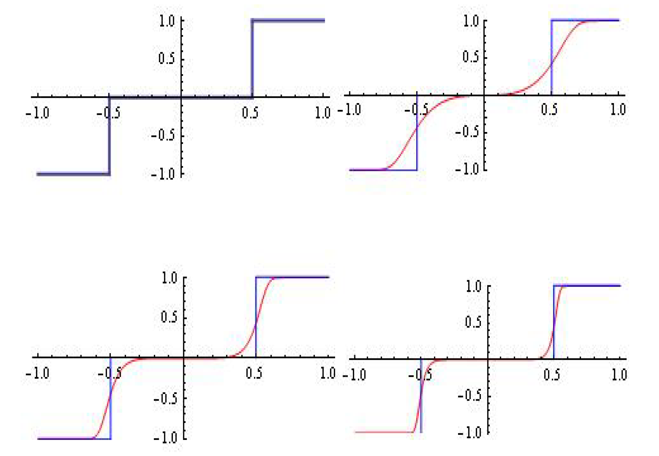
Figure 11.
Approximation by , : (a) ; (b) .

Figure 12.
Approximation of by : (a) : a) ; Hausdorff distance ; (b) : a) ; Hausdorff distance .

Figure 13.
The function -red.

Figure 14.
A “typical radiation pattern” for and .

Figure 15.
A “typical radiation pattern” for and .

Figure 16.
“Typical restrictions”.

Figure 17.
“Typical radiation patterns”.

Figure 18.
A typical diagram function with restrictions.

Figure 19.
The function for : (a) ; (b) .

Figure 20.
The function for : (a) ; (b) .

Publisher’s Note: MDPI stays neutral with regard to jurisdictional claims in published maps and institutional affiliations. |
© 2020 by the author. Licensee MDPI, Basel, Switzerland. This article is an open access article distributed under the terms and conditions of the Creative Commons Attribution (CC BY) license (http://creativecommons.org/licenses/by/4.0/).
Share and Cite
MDPI and ACS Style
Kyurkchiev, N. Some Intrinsic Properties of Tadmor–Tanner Functions: Related Problems and Possible Applications. Mathematics 2020, 8, 1963. https://0-doi-org.brum.beds.ac.uk/10.3390/math8111963
AMA Style
Kyurkchiev N. Some Intrinsic Properties of Tadmor–Tanner Functions: Related Problems and Possible Applications. Mathematics. 2020; 8(11):1963. https://0-doi-org.brum.beds.ac.uk/10.3390/math8111963
Chicago/Turabian StyleKyurkchiev, Nikolay. 2020. "Some Intrinsic Properties of Tadmor–Tanner Functions: Related Problems and Possible Applications" Mathematics 8, no. 11: 1963. https://0-doi-org.brum.beds.ac.uk/10.3390/math8111963
Note that from the first issue of 2016, this journal uses article numbers instead of page numbers. See further details here.