Mathematical Modeling and Simulation of a Gas Emission Source Using the Network Simulation Method

Abstract

A mathematical model for the simulation of the diffusion of the pollutants released from a point source is presented. All phenomena have been included, such as thermal and wind gradients, turbulence, fumigation, convective and diffusive effects, and atmospheric stabilities. To better understand the dynamics of these occurrences, the Network Simulation Method was used to provide the concentration of pollutants in three spatial coordinates. The model was simulated in open source software and validated with experimental data, satisfying the Hanna criteria. Additionally, this model selects for the appropriate expressions based on the physical phenomena that govern each case and allows for time-dependent data entry. The cases studied show the great coupling that exists between the variables of wind velocity and atmospheric stability for the pollutant diffusion. The model can be used for two important aims, to identify the behavior of the emission of pollutants, and to determine the concentration of a pollutant at various points, through an inverse problem, locating the source of the emission.

1. Introduction

Air pollution is understood as the existence of potentially harmful matter suspended in the air, which can be classified into basic chemical compounds (oxides of sulfur or nitrogen, carbon monoxide), particulate matter, high-risk radioactive compounds, or suspensions from a biological source, such as bacteria. All of which can produce harmful effects on the health of a population.

In all cases, the atmospheric dispersion of pollutants is essentially dependent on the air flow or wind velocity in the lower layers of the atmosphere. This dispersion represents an important environmental engineering problem in relation to the health of a population, particularly in areas where different pollution sources can be unhealthy and/or dangerous [1,2]. In city centers where the building density is high, emissions from chimneys accumulate in the open spaces between buildings due to the higher velocity of air flow and its turbulent nature in comparison with the open spaces.

For years, the main objective was to monitor the concentration of pollutants at each point in space and at each moment as a result of the dispersion caused by the movement of the atmospheric air in which the pollutants are suspended. The modeling of the atmospheric dispersion of pollutants elicits the mathematical and/or numerical study of these processes, seeking analytical or semi-analytical solutions that present increasingly accurate results.

After analyzing the behavior of smoke in numerous experiments for various types of emissions, Roberts [3], in 1923, proposed solutions for a steady state based on normal or Gaussian distributions of concentration, always under conditions of constant wind velocity and assuming that the coefficients of which the dispersion depended upon were constant. Thereby, it was possible to characterize the dispersions by means of standard deviations, giving rise to statistical models. All the expressions proposed by this author serve as the basis for more precise developments of passive dispersion models.

In 1953, Sutton [4] introduced the so-called Sutton diffusion coefficients, which can be considered as meteorological constants and decrease significantly with height, and the Sutton diffusion index which depends on the conditions of stability. Between 1961 and 1982, Pasquill [5,6,7] introduced a set of recommendations and guides for the determination of the different coefficients that depend on the class of atmospheric stability. Finally, Gifford [8], in 1961, modified the Pasquill model, giving rise to the Pasquill–Gifford model, introducing meteorological constants or dispersion coefficients, which represent the standard deviations in the wind directions [8,9]. Later, these coefficients were refined and discussed by Slade [10] and Turner [11].

However, the approximations provided are not devoid of error in their results. Thereby, the so-called gradient transfer models were introduced, such as the one presented in this work, which includes relationships that provide the changes of the diffusivities, of the temperatures, and of the wind velocity with the height and atmospheric stability, implementing increasingly complex equations that depend on a greater number of variables. These models lack an analytical solution and, hence, are solved by numerical simulations and validated with experimental data [12].

Therefore, the release of pollutants from a point sources poses a risk to the population, as there is an increase in concentration in a certain area, reaching in some cases, values higher than those recommended by international organizations. The use of the most accurate possible models that allow predicting the behavior of the pollutant once released allows for control and minimizes the risks for the population. In 2016, outdoor air pollution in both rural areas and cities around the world was reported to cause millions of premature deaths each year. The World Health Organization (WHO) estimates that approximately 58% of them were due to heart disease, 18% to pulmonary disease, and 6% to lung cancer [13].

The aims of this article are twofold: based on current bibliographies, we developed the most complete mathematical model to obtain the concentration of a pollutant that has been released at any point in space. Secondly, we developed an efficient and precise network method to solve the aforementioned mathematical model to be simulated in free software for circuit analysis, such as NgSpice [14], without linearization of the equations or making assumptions. Thus, the Network Simulation Method, the tool exploited in this work, has been used in numerous areas of engineering and science, demonstrating its effectiveness and reliability in addressing problems, such as dry friction, electrochemistry, oxidation processes, inverse problems, fluid flow transport, etc. [15,16,17,18,19,20,21].

2. Mathematical Model

The movement of pollutants released from a source involves numerous phenomena, such as turbulence, wind dragging, buoyancy forces, diffusive effects, etc. The governing equation that encompasses them is given by the following expression [12,22,23,24]:

$$\frac{\partial {\mathrm{c}}_{\mathrm{p}}}{\partial \mathrm{t}}+\frac{\partial \left({\mathrm{u}}_{\mathrm{x}}{\mathrm{c}}_{\mathrm{p}}\right)}{\partial \mathrm{x}}+\frac{\partial \left({\mathrm{u}}_{\mathrm{y}}{\mathrm{c}}_{\mathrm{p}}\right)}{\partial \mathrm{y}}+\frac{\partial \left({\mathrm{u}}_{\mathrm{z}}{\mathrm{c}}_{\mathrm{p}}\right)}{\partial \mathrm{z}}=\frac{\partial }{\partial \mathrm{x}}\left({\mathrm{K}}_{\mathrm{x}}\frac{\partial {\mathrm{c}}_{\mathrm{p}}}{\partial \mathrm{x}}\right)+\frac{\partial }{\partial \mathrm{y}}\left({\mathrm{K}}_{\mathrm{y}}\frac{\partial {\mathrm{c}}_{\mathrm{p}}}{\partial \mathrm{y}}\right)+\frac{\partial }{\partial \mathrm{z}}\left({\mathrm{K}}_{\mathrm{z}}\frac{\partial {\mathrm{c}}_{\mathrm{p}}}{\partial \mathrm{z}}\right)+{\mathrm{R}}_{\mathrm{c}}+{\mathrm{Q}}_{\mathrm{p}}$$

(1)

where c_p is the pollutant concentration in (µg/m³), u_x, u_y, and u_z are the wind velocities in the different space directions, x, y, and z, respectively, K_x, K_y, and K_z are the diffusivity parameters in the different directions of space, R_c (µg/m³ s) is the term of reaction or decay due to physicochemical reactions in the atmosphere that depend on each pollutant [25], and Q_p (µg/m³ s) is the term that implements the source or sink of the pollutant. This last variable represents the emission of the polluting gas, and can be a continuous emission and take a constant value over time; it can be a quick release, that is, of a short period of time; it can be an instantaneous emission; or it can be variable as a function of time.

Illustratively, Figure 1 is a schematic representation of the model showing the diffusion of the pollutant emitted by a point source in the direction of the wind, whose behavior is defined by Equation (1). Being an unbound medium, it is represented by a space large enough so that the pollutant diffusion does not reach the boundary. The different processes involved, as well as the boundary conditions, will be described in the next sections.

2.1. Atmospheric Stability

Stability conditions (which can be classified as neutral, stable or subadibatic, and unstable or superadibatic) define the atmospheric parameters. In neutral conditions, the buoyancy forces can be considered negligible while the drag forces of the wind on the earth’s surface, together with the effects derived from the change of direction and wind velocity with height, are the cause of turbulent energy transport. In unstable conditions, the buoyancy forces induced by heat flows are added to the above. Stable conditions occur at night, where the surface cools more than the air itself. Given the limitation of the division of stability into three groups, Pasquill [22] established a subdivision into atmospheric stability categories, whose relationship with stability is shown in the following table (

Table 1. Relationship between stability and the category of atmospheric stability [22].

Stability	Pasquill’s Stability Categories
Unstable (UB)	A, B, and C
Neutral (NL)	D
Stable (SB)	E, F, and G

):

The category of atmospheric stability is a function of different parameters, among which insolation, wind velocity, and cloudiness stand out (

Table 2. Pasquill’s stability categories depending on different parameters [22].

uref = 10 m (m/s)	Day			Night
	Insolation			Cloudiness
	Strong	Moderate	Slight	≥50%	<50%
<2	A	A-B	B	F	G
2–3	A-B	B	C	E	F
3–5	B	B-C	C	D	E
5–6	C	C-D	D	D	D
>6	C	D	D	D	D

) [22]. Wind velocity is usually measured at a reference height, v_ref, typically 10 m (z_ref), cloudiness is expressed as a percentage, and finally, insolation is a function of solar radiation and is established according to the following table (

Table 3. Relationship between solar radiation and insolation [26].

Solar Radiation (W/m2)	Insolation
>500	Strong
300–500	Moderate
<300	Slight

).

It is the solar radiation itself that establishes whether it is day or night. Thus, Table 2 can be expressed in terms of the three groups of stabilities: unstable, neutral, and stable (

Table 4. Atmospheric stability depending on different parameters.

vref = 10 m (m/s)	Day			Night
	Insolation			Cloudiness
	Strong	Moderate	Slight	≥50%	<50%
<2	UB	UB	UB	SB	SB
2–3	UB	UB	UB	SB	SB
3–5	UB	UB	UB	NL	SB
5–6	UB	UB-NL	NL	NL	NL
>6	UB	NL	NL	NL	NL

).

2.2. Vertical Heat Flux

This flux, H (W/m²), is obtained from the energy balance in the ground—the energy received from outside minus the energy emitted. The phenomenon is depreciable for neutral conditions, but it is significant for other conditions. The importance of this flux lies in the effect it has on turbulence through buoyancy effects. Some authors, such as Holtslag and van Ulden [27], considered the fraction of heat absorbed by the water that is invested in evaporation without changing the ground temperature, a phenomenon that, in turn, conditions the temperature of the outside air. Other authors, such as Clarke, established it through the following expression [28].

$$\mathrm{H}=0.4·\left({\mathrm{R}}_{\mathrm{solar}}-100\right)$$

(2)

where R_solar is the incoming solar radiation (W/m²). The importance of parameter H lies in its influence on turbulence, since if H > 0, the received energy is higher than that emitted (heating of the ground) and the atmosphere is superadibatic; if H ≤ 0, it is subadibatic (cooling of the ground); and finally, if H ≈ 0, it is a neutral atmosphere.

2.3. Wind Profiles

At levels close to the surface, the wind velocity is influenced by the effects of friction to a greater or lesser degree, being greater during the day, since these effects are determined by the topography and surface roughness (distribution and average height of the obstacles). The gradient decrease with height, showing a greater fall during the day. Thus, according to the American Society of Mechanical Engineers (ASME) [29], the velocity profiles have the shape indicated in Figure 2. The slope of these curves represents the inverse of the velocity gradient with height. By increasing the size of the obstacles, the velocities increase more slowly with the height.

As can be seen in Figure 2, there is turbulence of a mechanical origin associated with the horizontal components of the wind velocity, which is represented by the so-called friction velocity ${\mathrm{v}}_{*}$. As ${\mathrm{v}}_{*}$ increases, so does the turbulence and the intensity with which the wind components mix. Thus, in order to use the law of the wall $\frac{\partial \mathrm{v}}{\partial \mathrm{z}}=\frac{{\mathrm{v}}_{*}}{\mathrm{kz}}$, we need to determine $\frac{\partial \mathrm{v}}{\partial \mathrm{z}}$ or, what is the same, the velocity profile (v_z) as a function of the height (z) [22]. The constant k was determined by von Karman [30,31,32] and takes a value of 0.35. The velocity profile gives us the magnitude of the velocity at each height (v_z), which can be decomposed into its x and y components (u_x and u_y) through the wind angle with respect to the problem coordinate system, as seen in Figure 3. Regarding the vertical velocity of the wind, u_z, it is assumed to be practically zero [12,22].

To determine the velocity profile, the modified logarithmic or potential approximation can be used. The first one takes into account the predominant floating effects, introducing a Monin–Obukhov length (L) and a dimensionless length (z/L) known as the Monin–Obukhov parameter [33]. In this way, the law of the wall is modified as follows

$$\frac{\partial \mathrm{v}}{\partial \mathrm{z}}=\frac{{\mathrm{v}}_{*}}{\mathrm{kz}}{\mathsf{\varphi }}_{\mathrm{M}}=\frac{{\mathrm{v}}_{*}}{\mathrm{kz}}{\left(1+{\mathsf{\alpha }}_1\frac{\mathrm{z}}{\mathrm{L}}\right)}^{{\mathsf{\alpha }}_2}$$

(3)

where ϕ_M is a turbulent exchange coefficient due to mass. In this way, the wind profiles are based on atmospheric stabilities [31]. Thus, for neutral conditions, α₁ and α₂ take null values, 4.7 and 1, respectively, for stable conditions, and finally, −15 and −0.25, respectively, for unstable conditions [31]. Other authors, such as Dyer and Hicks [34] and Webb [35], have also adjusted these values.

When solving the integral, the integration constant (z_o) appears, which is called the roughness length. On aerodynamically rough surfaces, the velocity profiles are basically dependent on the roughness length, that is, on the distribution and height of rough elements (obstacles). This length takes different values depending on the terrain, such as in open spaces, forests, cities, and so on [22]. Thus, the solution for each of the atmospheric stabilities is given by the following:

$$\mathrm{v}=\frac{{\mathrm{v}}_{*}}{\mathrm{k}}\log \left(\frac{\mathrm{z}}{{\mathrm{z}}_{\mathrm{o}}}\right)\mathrm{neutral}\mathrm{stability},$$

(4)

$$\mathrm{v}=\frac{{\mathrm{v}}_{*}}{\mathrm{k}}\left(\log \left(\frac{\mathrm{z}}{{\mathrm{z}}_{\mathrm{o}}}\right)+4.7\frac{\mathrm{z}-{\mathrm{z}}_{\mathrm{o}}}{\mathrm{L}}\right)\mathrm{stable}\mathrm{stability},$$

(5)

$$\mathrm{v}=\frac{{\mathrm{v}}_{*}}{\mathrm{k}}\left(\log \left(\frac{\sqrt[4]{1-\frac{15\mathrm{z}}{\mathrm{L}}}-1}{\sqrt[4]{1-\frac{15\mathrm{z}}{\mathrm{L}}}+1}\right)-\log \left(\frac{\sqrt[4]{1-\frac{15{\mathrm{z}}_{\mathrm{o}}}{\mathrm{L}}}-1}{\sqrt[4]{1-\frac{15{\mathrm{z}}_{\mathrm{o}}}{\mathrm{L}}}+1}\right)+2{\mathrm{tg}}^{-1}\sqrt[4]{1-\frac{15\mathrm{z}}{\mathrm{L}}}-2{\mathrm{tg}}^{-1}\sqrt[4]{1-\frac{15{\mathrm{z}}_{\mathrm{o}}}{\mathrm{L}}}\right)\mathrm{unstable}\mathrm{stability}.$$

(6)

The potential approximation for the velocity profile is given by the following expression

$$\mathrm{v}={\mathrm{v}}_{\mathrm{ref}}{\left(\frac{\mathrm{z}}{{\mathrm{z}}_{\mathrm{ref}}}\right)}^{\mathrm{p}-\mathrm{index}}\mathrm{z}<{\mathrm{z}}_{\mathrm{ref}}$$

(7)

where the p-index is a parameter that depends on the Pasquill atmospheric stability category (

Table 5. The p-index for each category of atmospheric stability [22].

Pasquill Stability Category	p-Index
A	0.33
B	0.26
C	0.20
D, E	0.38
F	0.42
G	0.57

) [5].

2.4. Monin–Obukhov Length

This parameter, which includes all the parameters that influence the mechanical phenomena that occur in air, is used to determine the stability, and is considered as a measure (m) of the thickness of the layer of mechanical mixing close to the surface [33,36]. This length is given by:

$$\mathrm{L}=-\frac{{\mathrm{v}}_{*}{}^3{\mathsf{\rho }}_{\mathrm{a}}{\mathrm{c}}_{\mathrm{h},\mathrm{a}}{\mathrm{T}}_{\mathrm{r}}}{\mathrm{kgH}}$$

(8)

where c_h,a is the heat capacity of air and takes a value 1012 J/kgK, T_r is the air temperature (K), g is the acceleration of gravity, and ρ_a, is the air density (kg/m³). The Monin–Obukhov length takes positive values for a stable stability, negative values for an unstable one, and infinite for a neutral one.

2.5. Air Density

Jones [37] recommends expression (9) for the calculation of air density and for use in standards laboratories. Thereby, the air density depends on the relative humidity (RH), on the ambient temperature (T_a), and on the atmospheric pressure at ground level (P₀).

$${\mathsf{\rho }}_{\mathrm{a}}=\frac{0.4646}{{\mathrm{T}}_{\mathrm{a}}}\left(0.0075{\mathrm{P}}_0-0.003796·\mathrm{RH}·1.3146·{10}^9·{\mathrm{e}}^{-\frac{5315.56}{{\mathrm{T}}_{\mathrm{a}}}}\right).$$

(9)

2.6. Air Temperature Profile

There is also turbulence of a thermal origin, due to the vertical movements of the air caused by thermal gradients and to which atmospheric stability is traditionally associated. Mechanical and thermal turbulence occur simultaneously, contributing to the genesis and intensity of the global atmospheric turbulence. Given the turbulence of a thermal origin, air rises toward regions of lower pressure where it expands and cools. Under adiabatic or neutral conditions, the decrease rate in the dry air temperature with the height (dT/dz), one of the main constants in meteorology that is taken as a reference for real cases (not adiabatic), has the value dT/dz ≈ 0.01 °C/m or 1 °C/100 m [38,39]. The potential temperature of dry air (θ) is defined as that reached by an infinitesimal air volume when it is transported adiabatically from its pressure (P_z) to a reference pressure (surface pressure the earth, P₀). Its value, from the adiabatic relation T-P_z, is

$$\mathsf{\theta }=\mathrm{T}{\left(\frac{{\mathrm{P}}_0}{{\mathrm{P}}_{\mathrm{z}}}\right)}^{\frac{\mathsf{\gamma }-1}{\mathsf{\gamma }}}$$

(10)

where P_z (Pa) is the atmospheric pressure at different heights and γ is the adiabatic coefficient of air with a value of 1.4. From this expression, it can be deduced that, at ground level, the ambient temperature and the potential temperature take the same value. The pressure is related to temperature through the following relation

$${\mathrm{P}}_{\mathrm{z}}={\mathsf{\rho }}_{\mathrm{a}}{\mathrm{R}}_{\mathrm{g}}\mathrm{T}$$

(11)

where R_g is the ideal gas constant. Finally, the potential temperature profile is a function of stability and is given by the following expression [22]

$$\frac{\mathrm{d}\mathsf{\theta }}{\mathrm{dz}}=-\frac{\mathrm{H}}{{\mathrm{u}}_{*}{\mathsf{\rho }}_{\mathrm{a}}{\mathrm{c}}_{\mathrm{p},\mathrm{a}}{\mathrm{kz}}_{\mathrm{ref}}}{\mathsf{\varphi }}_{\mathrm{H}}=-\frac{\mathrm{H}}{{\mathrm{u}}_{*}{\mathsf{\rho }}_{\mathrm{a}}{\mathrm{c}}_{\mathrm{p},\mathrm{a}}{\mathrm{kz}}_{\mathrm{ref}}}{\left({\mathsf{\alpha }}_3+{\mathsf{\alpha }}_4\frac{\mathrm{z}}{\mathrm{L}}\right)}^{{\mathsf{\alpha }}_5}$$

(12)

where ϕ_H is a turbulent exchange coefficient due to heat [12]. In this way, the temperature profiles are a function of atmospheric stabilities [31]. Thus, for neutral and stable conditions, α₃, α_4, and α₅ take 0.74, 4.7, and 1, respectively, and for unstable conditions, 1.83, −16.44, and −0.5, respectively [31]. Again, when performing the integral, the integration constant (z_o) appears, which is called the roughness length.

2.7. Eddy Diffusivities

The horizontal diffusion coefficients, K_H, and vertical, K_V, (K_x = K_y = K_H and K_z = K_V), known as Eddy diffusivities, express the mechanical turbulent diffusivity. First, we will consider the vertical diffusivity as it is the most complex. For this case, a theory modified by dimensional arguments and stability considerations is applied that implies the convective boundary layer [2,12,40,41]. For this layer, the two main variables that control turbulence are the convective boundary layer depth, z_c, and the convective velocity scale, ${\mathrm{w}}_{*}$. Another important length for the calculation of diffusivities is the boundary layer height, H_b. The vertical transport of polluting material is dominated by turbulent diffusion under convective conditions that depends on different atmospheric conditions [12,22,40]. Thus, for stable conditions:

$${\mathrm{K}}_{\mathrm{V}}=\frac{{\mathrm{ku}}_{*}\mathrm{z}}{0.74+4.7\frac{\mathrm{z}}{\mathrm{L}}}{\mathrm{e}}^{-\mathrm{b}\mathsf{\eta }}$$

(13)

$$\mathsf{\eta }=\frac{\mathrm{z}}{\mathrm{L}}{\mathsf{\mu }}^{-1/2}\mathrm{and}\mathsf{\mu }=\frac{{\mathrm{u}}_{*}}{\left|\mathrm{fL}\right|}$$

(14)

where b is a constant with a value of 0.91, and f is the force or parameter of Coriolis (f = 2ωsenϕ ≈ 1.15 × 10⁻⁴ s⁻¹, where ϕ is the latitude and ω is the Earth angular velocity) [12,22]. For neutral conditions,

$${\mathrm{K}}_{\mathrm{V}}={\mathrm{u}}_{*}{\mathrm{kze}}^{\frac{-4\mathrm{z}}{{\mathrm{H}}_{\mathrm{b}}}}$$

(15)

$${\mathrm{H}}_{\mathrm{b}}=\mathrm{F}\frac{{\mathrm{u}}_{*}}{\mathrm{f}}$$

(16)

where F is a factor that varies between 0.25 and 1 and whose recommended value is 0.455 [12,22,40].

Finally, for unstable conditions [12,22,40,42],

$${\mathrm{K}}_{\mathrm{V}}={\mathrm{w}}_{*}{\mathrm{z}}_{\mathrm{c}}\left[2.5{\left(\mathrm{k}\frac{\mathrm{z}}{{\mathrm{z}}_{\mathrm{c}}}\right)}^{4/3}{\left(1-15\frac{\mathrm{z}}{\mathrm{L}}\right)}^{1/4}\right]0\le \frac{\mathrm{z}}{{\mathrm{z}}_{\mathrm{c}}}<0.05$$

(17)

$${\mathrm{K}}_{\mathrm{V}}={\mathrm{w}}_{*}{\mathrm{z}}_{\mathrm{c}}\left[0.021+0.408\frac{\mathrm{z}}{{\mathrm{z}}_{\mathrm{c}}}+1.352{\left(\frac{\mathrm{z}}{{\mathrm{z}}_{\mathrm{c}}}\right)}^2-4.096{\left(\frac{\mathrm{z}}{{\mathrm{z}}_{\mathrm{c}}}\right)}^3+2.56{\left(\frac{\mathrm{z}}{{\mathrm{z}}_{\mathrm{c}}}\right)}^4\right]0.05\le \frac{\mathrm{z}}{{\mathrm{z}}_{\mathrm{c}}}<0.6$$

(18)

$${\mathrm{K}}_{\mathrm{V}}={\mathrm{w}}_{*}{\mathrm{z}}_{\mathrm{c}}\left[0.2{\mathrm{e}}^{\left(6-10\frac{\mathrm{z}}{{\mathrm{z}}_{\mathrm{c}}}\right)}\right]0.6\le \frac{\mathrm{z}}{{\mathrm{z}}_{\mathrm{c}}}<1.1$$

(19)

$${\mathrm{K}}_{\mathrm{V}}=0.001{\mathrm{w}}_{*}{\mathrm{z}}_{\mathrm{c}}\frac{\mathrm{z}}{{\mathrm{z}}_{\mathrm{c}}}\ge 1.1$$

(20)

$${\mathrm{w}}_{*}={\mathrm{u}}_{*}{\left(-\frac{1}{\mathrm{k}}\frac{{\mathrm{z}}_{\mathrm{i}}}{\mathrm{L}}\right)}^{1/3}.$$

(21)

Under unstable conditions, the convective boundary layer depth, z_c, is the maximum value between two values [42].

$${\mathrm{z}}_{\mathrm{c}}=\max \left({\mathrm{h}}_1,{\mathrm{h}}_2\right)$$

(22)

$${\mathrm{h}}_1=0.3\frac{{\mathrm{u}}_{*}}{\mathrm{f}}$$

(23)

$${\mathrm{h}}_2\mathrm{is}\mathrm{the}\mathrm{lowest}\mathrm{value}\mathrm{where}\frac{\mathrm{d}\mathsf{\theta }}{\mathrm{dz}}\mathrm{takes}\mathrm{a}\mathrm{positive}\mathrm{value}.$$

(24)

Finally, for the case of horizontal diffusivity, K_H, the variation produces negligible changes in the concentration distribution, and so it is assigned a constant value of 50 m²/s [12,43,44].

2.8. Boundary Conditions

Except for the boundary condition on the ground, a first-class condition (Dirichlet type) is applied to the entire boundary as, with this, the imperviousness of pollutants is also ensured. A medium large enough value is taken so that it can be assumed as infinity. For the surface (z = 0), the boundary condition is of the greatest interest due to its location of the deposition of pollutants. In this case, a second-class non-homogeneous condition (Neumann type) is applied, governed by the equation

$$-{\mathrm{K}}_{\mathrm{v}}\frac{\partial {\mathrm{c}}_{\mathrm{p}}}{\partial \mathrm{z}}={\mathrm{v}}_{\mathrm{dep}}{\mathrm{c}}_{\mathrm{p}}\mathrm{z}=0$$

(25)

where v_dep is the deposition velocity that takes values in a range between 0.0004 and 0.075 m/s. For this work, a value of 0.02 m/s was taken [12].

3. The Network Model

The procedure to design a network model is described in Sánchez-Pérez et al. [17,45] and González-Fernández and Alhama [20]. To obtain a clearer design interpretation, the design will be described below. Firstly, the equivalence between the variable and the electric voltage, c_p ≡ V is established. Then, each of the distance variables, x, y, and z, are discretized in different volume elements. Applying the nomenclature in Figure 4, Equation (1) provides the following finite difference, Equation (26).

$$\begin{array}{l}\frac{\partial {\mathrm{c}}_{\mathrm{p}}}{\partial \mathrm{t}}+{\mathrm{u}}_{\mathrm{x}}\left[\frac{{\mathrm{c}}_{\mathrm{p}}{}_{\mathrm{l}+\frac{\Delta \mathrm{x}}{2},\mathrm{w},\mathrm{h}}-{\mathrm{c}}_{\mathrm{p}}{}_{\mathrm{l}-\frac{\Delta \mathrm{x}}{2},\mathrm{w},\mathrm{h}}}{\Delta \mathrm{x}}\right]+{\mathrm{u}}_{\mathrm{y}}\left[\frac{{\mathrm{c}}_{\mathrm{p}}{}_{\mathrm{l},\mathrm{w}+\frac{\Delta \mathrm{y}}{2},\mathrm{h}}-{\mathrm{c}}_{\mathrm{p}}{}_{\mathrm{l},\mathrm{w}-\frac{\Delta \mathrm{y}}{2},\mathrm{h}}}{\Delta \mathrm{y}}\right]-\left[\frac{{\mathrm{c}}_{\mathrm{p}}{}_{\mathrm{l}+\frac{\Delta \mathrm{x}}{2},\mathrm{w},\mathrm{h}}-{\mathrm{c}}_{\mathrm{p}}{}_{\mathrm{l}-\frac{\Delta \mathrm{x}}{2},\mathrm{w},\mathrm{h}}}{\frac{\Delta {\mathrm{x}}^2}{2{\mathrm{K}}_{\mathrm{H}}}}\right]-\left[\frac{{\mathrm{c}}_{\mathrm{p}}{}_{\mathrm{l},\mathrm{w}+\frac{\Delta \mathrm{y}}{2},\mathrm{h}}-{\mathrm{c}}_{\mathrm{p}}{}_{\mathrm{l},\mathrm{w}-\frac{\Delta \mathrm{y}}{2},\mathrm{h}}}{\frac{\Delta {\mathrm{y}}^2}{2{\mathrm{K}}_{\mathrm{H}}}}\right]\\ -\left[\frac{{\mathrm{c}}_{\mathrm{p}}{}_{\mathrm{l},\mathrm{w},\mathrm{h}+\frac{\Delta \mathrm{z}}{2}}-{\mathrm{c}}_{\mathrm{p}}{}_{\mathrm{l},\mathrm{w},\mathrm{h}-\frac{\Delta \mathrm{z}}{2}}}{\frac{\Delta {\mathrm{z}}^2}{2{\mathrm{K}}_{\mathrm{v}}}}\right]-\left[\frac{{\mathrm{K}}_{\mathrm{v},\mathrm{l},\mathrm{w},\mathrm{h}+\frac{\Delta \mathrm{z}}{2}}-{\mathrm{K}}_{\mathrm{v},\mathrm{l},\mathrm{w},\mathrm{h}-\frac{\Delta \mathrm{z}}{2}}}{\Delta \mathrm{z}}\right]\left[\frac{{\mathrm{c}}_{\mathrm{p}}{}_{\mathrm{l},\mathrm{w},\mathrm{h}+\frac{\Delta \mathrm{z}}{2}}-{\mathrm{c}}_{\mathrm{p}}{}_{\mathrm{l},\mathrm{w},\mathrm{h}-\frac{\Delta \mathrm{z}}{2}}}{\Delta \mathrm{z}}\right]-{\mathrm{R}}_{\mathrm{c}}-\mathrm{Q}\\ =0\end{array}$$

(26)

where the subscripts l, w, and h are the space coordinates. To develop Equation (26), we considered that the wind speed practically does not vary with respect to the x and y coordinates and takes a null value in the z direction. The K_H variable will also take a constant value.

Following the scheme of Figure 5, each addend of Equation (26) is an electric current that is balanced at a central node. The fourth, fifth, and sixth addends, that is, the second derivatives, are implemented as simple resistors, R_x, R_y, and R_z, for each of the spatial coordinates, respectively, where ${\mathrm{R}}_{\mathrm{x}}=\frac{\Delta {\mathrm{x}}^2}{2{\mathrm{K}}_{\mathrm{H}}}$, ${\mathrm{R}}_{\mathrm{y}}=\frac{\Delta {\mathrm{y}}^2}{2{\mathrm{K}}_{\mathrm{H}}}$, and ${\mathrm{R}}_{\mathrm{z}}=\frac{\Delta {\mathrm{z}}^2}{2{\mathrm{K}}_{\mathrm{v}}}$, and the time derivative are implemented as a capacitor (C_r,i,j,k).

The rest of the addends are implemented as controlled current sources; however, the last two terms connect from earth to the central node and the terms that imply movement in one direction, wind velocity or diffusivity, connect from one end of the cell to the other, since they imply a direction and a sense. Thus, the terms of a chemical reaction and source or sink of pollutants are given by ${\mathrm{I}}_{{\mathrm{R}}_{\mathrm{c}}}={\mathrm{R}}_{\mathrm{c}}\left({\mathrm{G}}_{{\mathrm{R}}_{\mathrm{c}}}\right)$ and ${\mathrm{I}}_{\mathrm{Q}}=\mathrm{Q}\left({\mathrm{G}}_{\mathrm{Q}}\right)$, respectively. The terms of velocity and diffusivity are given by ${\mathrm{I}}_{{\mathrm{u}}_{\mathrm{x}}}={\mathrm{u}}_{\mathrm{x}}\left[\frac{{\mathrm{c}}_{\mathrm{p}}{}_{\mathrm{l}+\frac{\Delta \mathrm{x}}{2},\mathrm{w},\mathrm{h}}-{\mathrm{c}}_{\mathrm{p}}{}_{\mathrm{l}-\frac{\Delta \mathrm{x}}{2},\mathrm{w},\mathrm{h}}}{\Delta \mathrm{x}}\right]\left({\mathrm{G}}_{{\mathrm{u}}_{\mathrm{x}}}\right)$ for x-wind velocity,${\mathrm{I}}_{{\mathrm{u}}_{\mathrm{y}}}={\mathrm{u}}_{\mathrm{y}}\left[\frac{{\mathrm{c}}_{\mathrm{p}}{}_{\mathrm{l},\mathrm{w}+\frac{\Delta \mathrm{y}}{2},\mathrm{h}}-{\mathrm{c}}_{\mathrm{p}}{}_{\mathrm{l},\mathrm{w}-\frac{\Delta \mathrm{y}}{2},\mathrm{h}}}{\Delta \mathrm{y}}\right]\left({\mathrm{G}}_{{\mathrm{u}}_{\mathrm{y}}}\right)$ for y-wind velocity, and finally, ${\mathrm{I}}_{{\mathrm{k}}_{\mathrm{v}}}=\left[\frac{{\mathrm{K}}_{\mathrm{v},\mathrm{l},\mathrm{w},\mathrm{h}+\frac{\Delta \mathrm{z}}{2}}-{\mathrm{K}}_{\mathrm{v},\mathrm{l},\mathrm{w},\mathrm{h}-\frac{\Delta \mathrm{z}}{2}}}{\Delta \mathrm{z}}\right]\left[\frac{{\mathrm{c}}_{\mathrm{p}}{}_{\mathrm{l},\mathrm{w},\mathrm{h}+\frac{\Delta \mathrm{z}}{2}}-{\mathrm{c}}_{\mathrm{p}}{}_{\mathrm{l},\mathrm{w},\mathrm{h}-\frac{\Delta \mathrm{z}}{2}}}{\Delta \mathrm{z}}\right]\left({\mathrm{G}}_{{\mathrm{k}}_{\mathrm{v}}}\right)$.

The rest of the expressions are implemented as controlled voltage sources that allow the inclusion of conditioning factors and variable values. These sources, depending on each scenario, choose between the values assigned to Table 1, Table 2, Table 3 and Table 4 and select the values for expressions (4) to (7) and (12). Furthermore, they use the appropriate expression between (13), (15), and (17) to (20) for each case or determine the convective boundary layer depth by implementing a conditional code in the source. By allowing these sources to change the values, we can introduce different values that change with time, such as solar radiation, wind velocity, and temperature at the reference height, etc., through expressions or fixed values for a certain time. Finally, the release source and the physical-chemical reactions are implemented as controlled current sources.

The boundary conditions are implemented as very high value resistors, except for that of the ground, which uses a controlled current source for its implementation. Being an unbounded medium, the meshing must be sufficiently extensive so that the boundary does not influence the concentrations in the positions where we want to know them. As a criterion to choose a suitable mesh, the one where the concentrations in the boundary are practically zero is taken. Finally, to simulate the model, a circuit simulation software, such as NgSpice is used [14,46].

4. Validation and Results

To validate the model, we compared it with the experimental results obtained from the literature. Ma et al. [47] used, in their experimental tests, a gaseous pollutant whose density was similar to that of ambient air, so as to not be affected by gravity. These contaminants are known as neutrally-buoyant pollutants [47,48]. In addition, the pollutant does not transform into another compound, so there are no physicochemical reactions. Due to the significant number of variables that must be measured and that also influence the concentration measurement (variable wind velocity and direction, temperature, etc.), the experimental values are not exempt from error. This methodology, derived from the Prairie Grass experimental data, was used to verify and optimize the different emission methods [47,49]. Thus,

Table 6. Input data of the problem.

Variable	Case 1
Emission rate (g/s)	56.5
Emission source height (m)	0.46
Wind velocity (m/s)	2.87
Wind direction (°)	184
Temperature (°C)	27.3
Monin–Obukhov Length (m)	61.54
Pasquill’s stability	E

shows the input data of the problem [47].

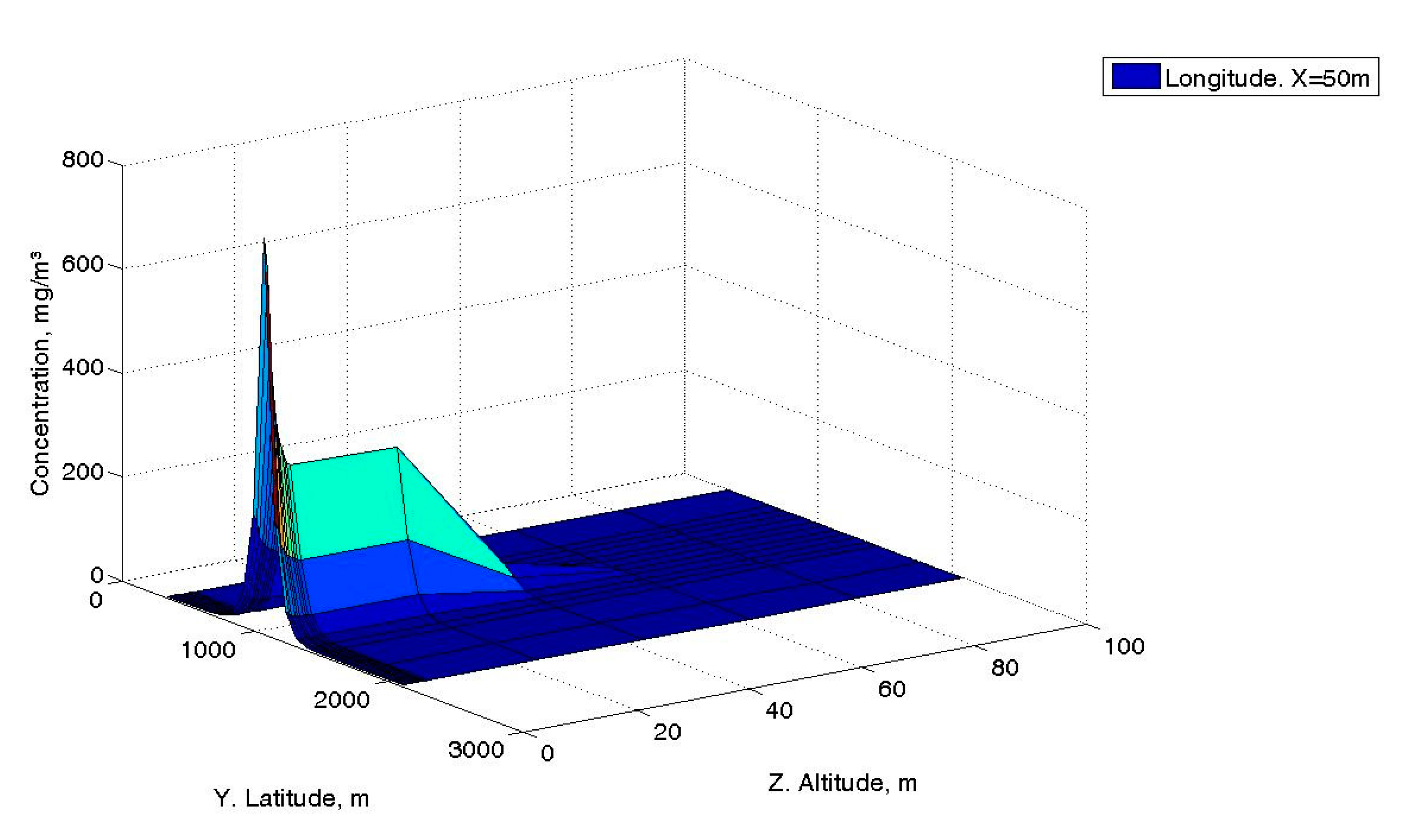
Ma et al. [47] indicated in their article that they used a point source of continuous emission. Therefore, in the simulation, we adjusted the time following the criteria given by Hanna [39,47,48]. The simulation presents a scenario composed of a volume of 12,000 × 2500 × 100 m using a fine mesh of 2000 × 800 × 5 m close to the emission source. Figure 6, Figure 7, Figure 8, Figure 9 and Figure 10 show the results of the simulation. Figure 6 and Figure 7 are 3D representations with concentrations and two spatial coordinates. Thus, Figure 6 shows the concentration distribution at 0.50 m of height for a section of 12,000 for the x-coordinate and 2500 m for the y-coordinate. As can be seen, the concentration falls rapidly to very low values in the first 1000 m. Figure 7 shows the distribution in the y and z coordinates, setting x to a value of 50 m. This figure shows that the concentration starting from 40 m decays rapidly. For both figures, the concentration distribution on the y axis is symmetric with respect to the emission source. The rest of the figures are representations of the concentrations against a spatial coordinate.

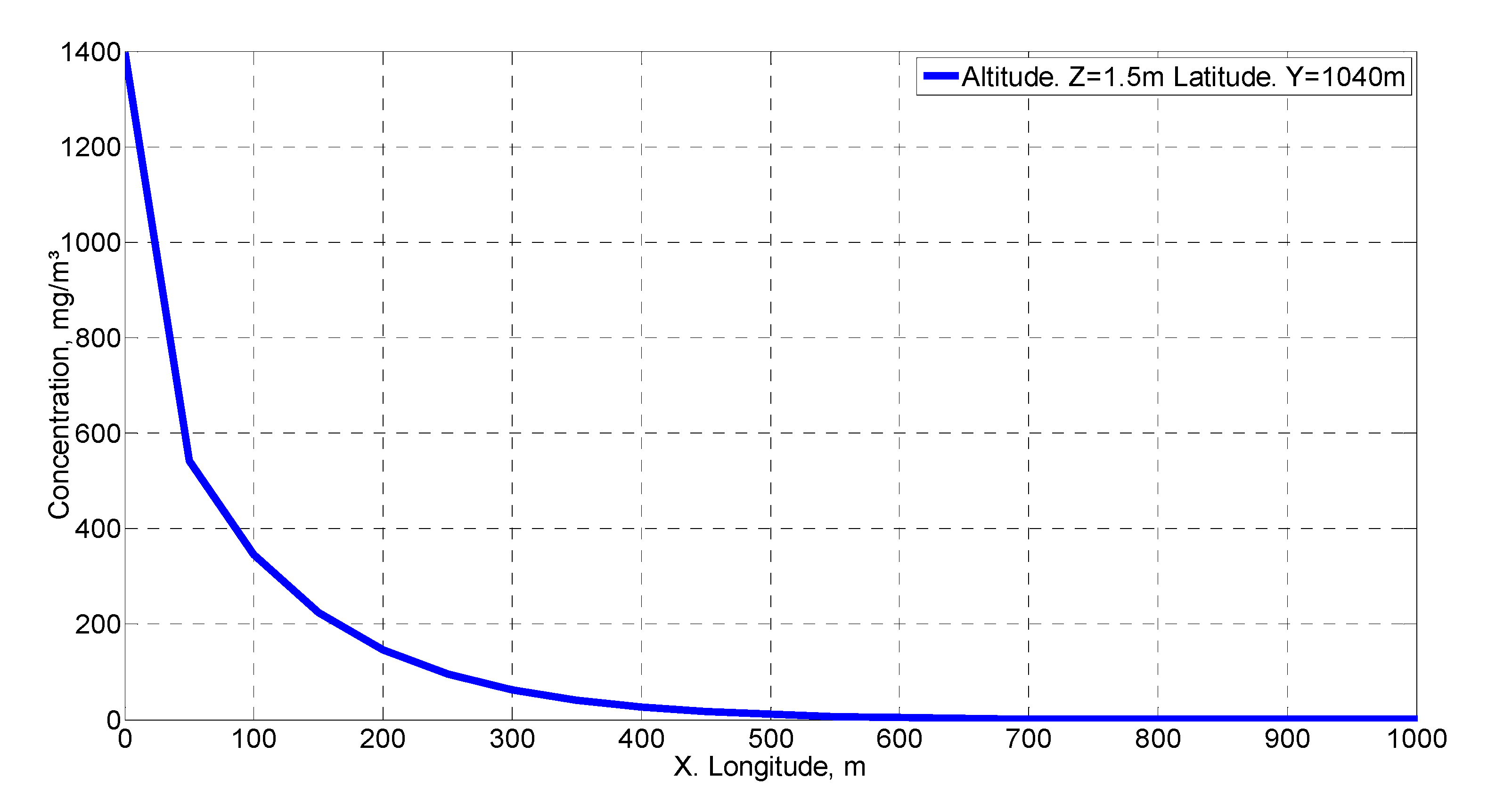
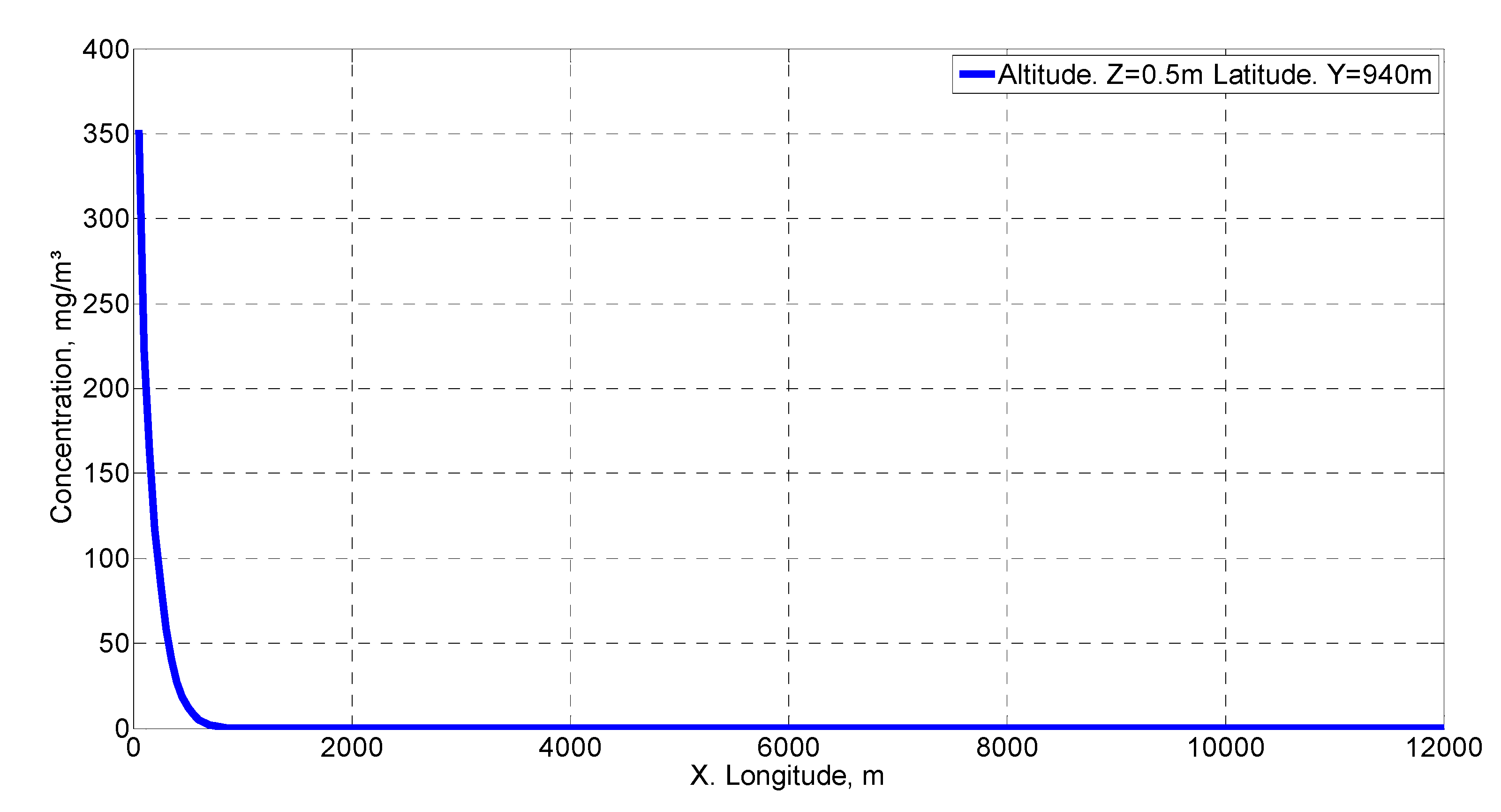
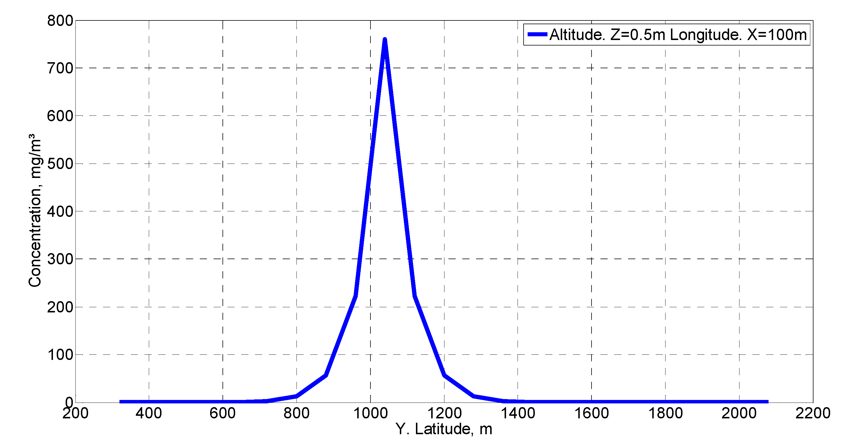
Figure 8 shows the concentration distribution on the x-axis in the wind direction with the same coordinates as the source for x and y. This figure has been used for the validation of the methodology used according to the criteria given by Hanna [39]. Figure 9 illustrates the concentration distribution on the x-axis in the direction of the wind at the same height and at 100 m from the emission source at the y-coordinate. Finally, Figure 10 shows a cross section to the wind direction at 100 m in the x-coordinate and at the same height as the emission source. These last two figures are the ones that best allow us to observe the behavior of the concentration distribution, particularly the one represented in the wind direction.

Finally,

Table 7. Simulated and experimental data comparison for Case 1.

Distance m	Experimental Data mg/m3	Simulated Concentration mg/m3	Ratio
50	650	542.3	0.83
100	275	346.3	1.26
200	86	146.7	1.71
400	26	26.7	1.03

shows the comparison of the results between those obtained by simulation and the experimental values including the ratio or degree of prediction. These values present a ratio that meets the factor of two of the observed values, satisfying the criterion of Hanna to evaluate a model as satisfactory [39,50]. The closer the ratio is to the unit, the better the prediction. The worst prediction occurred at 200 m, possibly because the measurement was wrong due to an experimental error, even though the value meets Hanna’s criteria [39].

Next, we studied different boundary conditions, both for the wind velocity and for the atmospheric Pasquill’s stability categories. First, Case 2 shows a day with moderate insolation and a very low wind velocity; however, for Case 3, it occurs at night with a high wind velocity (

Table 8. The input data for Cases 2, 3, and 4.

Variable	Case 2	Case 3	Case 4
Emission rate (g/s)	56.5	56.5	-
Mass release (g)	-	-	1695
Emission source height (m)	0.46	0.46	0.46
Wind velocity (m/s)	1	6	2.87
Wind direction (°)	184	184	184
Temperature (°C)	27.3	27.3	27.3
Insolation or period	Strong	Night	Night
Pasquill’s stability	B	D	E

). In both Cases, the emission is continuous. Finally, Case 4 represents an instantaneous emission of one minute where half the mass that is released in Case 1 per minute is released.

The first case studied (Case 1), which was used for the validation of the model, corresponds to a light breeze with a moderately stable stability category that can produce a fumigation effect [22,51]. As shown in Figure 7, this effect produced a higher concentration than in the rest of the cases studied. The second case (Case 2) corresponds to a practically calm wind with a moderately unstable stability category that produces a dispersion of the pollutant known as “looping”, favoring convection phenomena [22,51]. For the height studied, this effect decreased the concentration with respect to the previous case (Figure 11). Finally, Case 3 corresponds to a wind that raises dust or shakes small trees with a neutral stability category that produces a “coning” type dispersion [22,51]. This combination makes the concentration even lower for the position studied than in the previous cases (Figure 12).

Case 2 would be expected to present a higher concentration near the source as it has a lower wind velocity. However, the possible combination of the fumigation effect of stable conditions and the convective phenomena of its stability make its concentration lower than in Case 1. Finally, if cases 1 and 4 are compared, at positions close to the emission source, approximately half the concentration is obtained in Case 4 (Figure 13) when compared with Case 1 (Figure 8). In more distant positions, the concentration decreased more rapidly in the instantaneous case, possibly by the amount of mass emitted and the release time. Clearly, with increasing time, the concentration of Case 4 decreased as this was an instantaneous emission.

5. Conclusions

This work presents a mathematical model of the diffusion of pollutants emitted from a point source, based on current bibliographies, which encompasses phenomena, such as turbulence, buoyancy forces, drag forces, thermal gradients, and diffusive effects. This model was solved using a numerical model, built using the Network Simulation Method, without linearization of the equations or making assumptions. All the conditioning factors of the mathematical model were implemented, allowing for the choice between the most appropriate equations at all times. In addition, this allows the input values to be variable over time, such as the velocity and direction of the wind, temperature, and atmospheric pressure. The proposed model allows the introduction of pollutant emissions as a function of time, including both instantaneous and continuous emissions with a constant emission value. The model, which was validated with experimental data, meets the criterion of Hanna to evaluate a model as satisfactory. The results obtained from the simulation allow for the attainment of the concentration in a three-dimensional space of a pollutant that has been released by a point source. This model also allows for the representation of the concentration in one or two spatial coordinates, which facilitates understanding of the behavior of the pollutant.

The cases studied demonstrated the great influence that wind velocity and atmospheric stability have on the dispersion of a pollutant, since, a priori, it could be expected that the lower the wind velocity, the greater the concentration near the source of emission. However, the convective phenomena for unstable stability or the possible fumigation effect for stable conditions can make the concentration lower.

The use of precise models in the diffusion of pollutants has two important applications, the first to know, a priori, the behavior of the emission of pollutants, and the second, to know the concentration of a pollutant at various points, through an inverse problem, locating the emission source.

References

- ASHRAE (American Society of Heating Refrigeration and Air-Conditioning Engineers). Building air intake and exhaust design. In ASHRAE Handbook Heating, Ventiating and Air-Conditioning Aplications; ASHRAE: Atlanta, GA, USA, 2007. [Google Scholar]
- Lateb, M.; Meroney, R.N.; Yataghene, M.; Fellouah, H.; Saleh, F.; Boufadel, M.C. On the use of numerical modelling for near-field pollutant dispersion in urban environments—A review. Environ. Pollut. 2016, 208, 271–283. [Google Scholar] [CrossRef] [Green Version]
- Roberts, O.F. The theoretical scattering of smoke in a turbulent atmosphere. Proc. R. Soc. London. Ser. A Contain. Pap. Math. Phys. Character 1923, 104, 640–654. [Google Scholar]
- Sutton, O.G. Micrometeorology; McGraw-Hill: New York, NY, USA, 1953. [Google Scholar]
- Pasquill, F. The Estimation of the Dispersion of Windborne Material. Meteorol. Mag. 1961, 90, 33–40. [Google Scholar]
- Pasquill, F. Some observed properties of medium-scale diffusion in the atmosphere. Q. J. R. Meteorol. Soc. 1962, 88, 70–79. [Google Scholar] [CrossRef]
- Pasquill, F. Atmospheric Dispersion Models for Environmental Pollution Applications. In Lectures on Air Pollution and Environmental Impact Analyses; American Meteorological Society: Boston, MA, USA, 1982; ISBN 978-1-935704-23-2. [Google Scholar]
- Gifford, F. Small-scale turbulent diffusion in the atmosphere. Nature 1961, 190, 248. [Google Scholar] [CrossRef]
- Turner, D.B. A Diffusion Model for an Urban Area. J. Appl. Meteorol. 1964, 3, 83–91. [Google Scholar] [CrossRef]
- Slade, D.H. (Ed.) Meteorology and atomic energy 1968. Air Resources Laboratory, ESSA, for USAEC Division of Technical Information. Pp. 445; 234 Figures; 60 Tables. $3. Q. J. R. Meteorol. Soc. 1969, 95, 446. [Google Scholar] [CrossRef]
- Turner, J.S. Buoyancy effects in fluids. In Buoyancy Effects in Fluids; Cambridge University Press: Cambridge, UK, 1973. [Google Scholar]
- Ku, J.Y.; Rao, S.T.; Rao, K.S. Numerical simulation of air pollution in urban areas: Model development. Atmos. Environ. 1987, 21, 201–212. [Google Scholar] [CrossRef]
- WHO. Ambient (Outdoor) Air Pollution. Available online: https://www.who.int/en/news-room/fact-sheets/detail/ambient-(outdoor)-air-quality-and-health (accessed on 20 September 2020).
- Sourceforge. NgSpice. Available online: http://ngspice.sourceforge.net/index.html (accessed on 20 September 2020).
- Sánchez Pérez, J.F.; Moreno, J.A.; Alhama, F. Numerical Simulation of High-Temperature Oxidation of Lubricants Using the Network Method. Chem. Eng. Commun. 2015, 202, 982–991. [Google Scholar] [CrossRef]
- Sánchez, J.F.; Alhama, F.; Moreno, J.A. An efficient and reliable model based on network method to simulate CO2 corrosion with protective iron carbonate films. Comput. Chem. Eng. 2012, 39, 57–64. [Google Scholar] [CrossRef]
- Sánchez-Pérez, J.F.; Marín, F.; Morales, J.L.; Cánovas, M.; Alhama, F. Modeling and simulation of different and representative engineering problems using network simulation method. PLoS ONE 2018, 13, e0193828. [Google Scholar] [CrossRef] [PubMed] [Green Version]
- García-Ros, G.; Alhama, I.; Cánovas, M. Powerful software to Simulate soil Consolidation problems with prefabricated Vertical Drains. Water 2018, 10, 242. [Google Scholar] [CrossRef] [Green Version]
- Zueco, J.; Alhama, F. Inverse estimation of temperature dependent emissivity of solid metals. J. Quant. Spectrosc. Radiat. Transf. 2006, 101, 73–86. [Google Scholar] [CrossRef]
- González-Fernández, C.F.; Alhama, F. Heat Transfer and the Network Simulation Method; Horno, J., Ed.; Transworld Research Network: Trivandrum, India, 2001. [Google Scholar]
- Sánchez-Pérez, J.F.; Nicolas, J.A.M.; Alhama, F.; Canovas, M. Study of transition zones in the carbon monoxide catalytic oxidation on platinum using the network simulation method. Mathematics 2020, 8, 1413. [Google Scholar] [CrossRef]
- Frank, L. Lees’ Loss Prevention in the Process Industries; Elsevier: Amsterdam, The Netherlands, 2012. [Google Scholar]
- Moradpour, M.; Afshin, H.; Farhanieh, B. A numerical investigation of reactive air pollutant dispersion in urban street canyons with tree planting. Atmos. Pollut. Res. 2017, 8, 253–266. [Google Scholar] [CrossRef]
- Albani, R.A.S.; Duda, F.P.; Pimentel, L.C.G. On the modeling of atmospheric pollutant dispersion during a diurnal cycle: A finite element study. Atmos. Environ. 2015, 118, 19–27. [Google Scholar] [CrossRef]
- Seinfeld, J.H.; Pandis, S.N. Atmospheric Chemistry and Physics: From Air Pollution to Climate Change; Wiley: Hoboken, NJ, USA, 2006. [Google Scholar]
- Rabeiy, R.E. Spatial Modeling of Heavy Metal Pollution of Forest Soils in a Historical Mining Area Using Geostatistical Methods and Air Dispersion Modeling; Technischen Universität Clausthal: Clausthal-Zellerfeld, Germany, 2010. [Google Scholar]
- Holtslag, A.A.M.; Van Ulden, A.P. A simple scheme for daytime estimates of the surface fluxes from routine weather data. J. Clim. Appl. Meteorol. 1983, 22, 517–529. [Google Scholar] [CrossRef]
- Clarke, R.H. A Model for Short and Medium Range Dispersion of Radionuclides Released to the Atmosphere; National Radiological Protection Board: Harwell, UK, 1979. [Google Scholar]
- ASME PTC Committee. Standard for Verification and Validation in Computational Fluid Dynamics and Heat Transfer: ASME V&V 20; American Society of Mechanical Engineers: New York, NY, USA, 2009; ISBN 9780791832097. Available online: https://www.asme.org/codes-standards/find-codes-standards/v-v-20-standard-verification-validation-computational-fluid-dynamics-heat-transfer (accessed on 20 september 2020).
- von Karman, T. Progress in the Statistical Theory of Turbulence. Proc. Natl. Acad. Sci. USA 1948, 34, 530–539. [Google Scholar] [CrossRef] [Green Version]
- Businger, J.A.; Wyngaard, J.C.; Izumi, Y.; Bradley, E.F. Flux- profile relationships in the atmospheric surface layer. J. Atmos. Sci. 1971, 28, 181–189. [Google Scholar] [CrossRef]
- Nagib, H.M.; Chauhan, K.A. Variations of von Kármán coefficient in canonical flows. Phys. Fluids 2008. [Google Scholar] [CrossRef]
- Monin, A.S.; Obukhov, A.M. Basic laws of turbulent mixing in the surface layer of the atmosphere. Contrib. Geophys. Inst. Acad. Sci. USSR 1954, 151, 163–187. [Google Scholar]
- Dyer, A.J.; Hicks, B.B. Flux-gradient relationships in the constant flux layer. Q. J. R. Meteorol. Soc. 1970, 96, 715–721. [Google Scholar] [CrossRef]
- Webb, E.K. Profile relationships: The log-linear range, and extension to strong stability. Q. J. R. Meteorol. Soc. 1970, 96, 67–90. [Google Scholar] [CrossRef]
- Leelőssy, Á.; Molnár, F.; Izsák, F.; Havasi, Á.; Lagzi, I.; Mészáros, R. Dispersion modeling of air pollutants in the atmosphere: A review. Cent. Eur. J. Geosci. 2014, 6, 257–278. [Google Scholar] [CrossRef]
- Jones, F.E. Air density equation and the transfer of the mass unit. J. Res. Natl. Bur. Stand. 1978, 83, 419. [Google Scholar] [CrossRef]
- Sutton, O.G. A theory of eddy diffusion in the atmosphere. Proc. R. Soc. A 1932, 135, 143–165. [Google Scholar]
- Hanna, S.R. Handbook on Atmospheric Diffusion Models; U.S. Department of Commerce: Washington, DC, USA, 1981.
- Shir, C.C. A Preliminary Numerical Study of Atmospheric Turbulent Flows in the Idealized Planetary Boundary Layer. J. Atmos. Sci. 1973, 30, 1327–1339. [Google Scholar] [CrossRef] [Green Version]
- Dimitrova, R.; Fernando, H.J.S.; Silver, Z.; Leo, L.S.; Hocut, C.; Zsedrovits, T.; Di Sabatino, S. Modification of the Yonsei university boundary layer scheme in the WRF model for stable conditions. In Proceedings of the HARMO 2014—16th International Conference on Harmonisation within Atmospheric Dispersion Modelling for Regulatory Purposes, Varna, Bulgaria, 8–11 September 2014. [Google Scholar]
- Aliabadi, A.A.; Staebler, R.M.; De Grandpré, J.; Zadra, A.; Vaillancourt, P.A. Comparison of Estimated Atmospheric Boundary Layer Mixing Height in the Arctic and Southern Great Plains under Statically Stable Conditions: Experimental and Numerical Aspects. Atmos. Ocean 2016, 54, 60–74. [Google Scholar] [CrossRef]
- Reynolds, S.D.; Sienfeld, J.H.; Roth, P.M. Mathematical modeling of photochemical air pollution—1. formulation of the model. Atmos. Environ. 1973, 7, 1033–1061. [Google Scholar] [CrossRef]
- McRae, G.J.; Goodin, W.R.; Seinfeld, J.H. Development of a second-generation mathematical model for Urban air pollution-I. Model formulation. Atmos. Environ. 1982, 16, 679–696. [Google Scholar] [CrossRef]
- Sanchez Perez, J.F.; Conesa, M.; Alhama, I. Solving ordinary differential equations by electrical analogy: A multidisciplinary teaching tool. Eur. J. Phys. 2016, 37, 065703. [Google Scholar] [CrossRef]
- Nagel, L.W. SPICE2: A Computer Program To Simulate Semiconductor Circuits. Ph.D. Thesis, University California, Berkeley, CA, USA, 1975. [Google Scholar]
- Ma, D.; Deng, J.; Zhang, Z. Comparison and improvements of optimization methods for gas emission source identification. Atmos. Environ. 2013, 81, 188–198. [Google Scholar] [CrossRef]
- Jones, R.; Lehr, W.; Simecek-Beatty, D.; Reynolds, R.M. Aloha ® (Areal Locations of Hazardous Atmospheres) 5.4.4; U.S. Department of Commerce: Washington, DC, USA, 2013.
- Barad, M.L. Project Prairie Grass: A Field Program in Diffusion Vol II; Geophysical Research Paper Bedford; Air Force Cambridge Research Center: Cambridge, MA, USA, 1958. [Google Scholar]
- Goyal, P.; Kumar, A. Mathematical Modeling of Air Pollutants: An Application to Indian Urban City. Air Qual. Models Appl. 2011. [Google Scholar] [CrossRef] [Green Version]
- Gifford, F.A. Turbulent diffusion-typing schemes: A review. Nucl. Saf. 1976, 17, 68–86. [Google Scholar]
Figure 1.
Schematic representation of the model.
Figure 2.
The wind velocity profile [22].
Figure 3.
The wind velocity components at a given height z.
Figure 4.
Nomenclature of volume elements.
Figure 5.
Network model of a volume element.
Figure 6.
The concentration distribution at a height of 0.46 m for a section of 12,000 m of longitude and 2500 m of latitude for Case 1.
Figure 7.
The concentration distribution at a longitude of 50 m for a section of 100 heights and 2500 m of latitude for Case 1.
Figure 8.
The concentration distribution on the x-axis in the wind direction with the same coordinates as the source for x and y for Case 1.
Figure 9.
The concentration distribution at 0.50 m of height and a latitude of 940 m for Case 1.
Figure 10.
The concentration distribution at 0.50 m of height and a longitude of 100 m for Case 1.
Figure 11.
The concentration distribution on the x-axis in the wind direction with the same coordinates as the source for x and y for Case 2.
Figure 12.
The concentration distribution on the x-axis in the wind direction with the same coordinates as the source for x and y for Case 3.
Figure 13.
The concentration distribution on the x-axis in the wind direction with the same coordinates as the source for x and y for Case 4.