Risk Appetite and Jumps in Realized Correlation

Abstract

This paper examines the role of non-cash flow factors over correlation jumps in financial markets. Utilizing time-varying risk aversion measure as a proxy for investor sentiment and the cross-quantilogram method applied to intraday data, we show that risk aversion captures significant predictive power over realized stock-bond correlation jumps at different quantiles and lags. The predictive relation between correlation jumps and time-varying risk aversion is found to be asymmetric, as we detect a heterogeneous dependence pattern across different quantiles and lag orders. Our findings underline the importance of non-cash flow factors over correlation jumps, highlighting the role of behavioral factors in optimal portfolio allocations and the effectiveness of diversification strategies.

1. Introduction

Correlations amongst asset returns in a portfolio are critical for the effectiveness of diversification strategies, particularly during periods of market downturns, which is when diversification is needed the most [1]. Considering that diversification in a portfolio has traditionally been measured by the pairwise correlations of assets in the portfolio, any abrupt changes in correlation patterns could leave investors under-diversified, resulting in significant economic losses in portfolio valuations [1,2,3]. Accordingly, over the past decade, what has been of significance is understanding how macroeconomic changes affect the time variation in the stock-bond market correlations, as these two asset classes constitute major components of traditional portfolio allocations. The literature offers several approaches suggesting how to explore the economic determinants of the time variation in stock-bond correlations [4], since correlations have been shown to exhibit significant variability due to market conditions in the post-war period [5].

Towards this direction, a number of empirical studies in the literature report asymmetric patterns in return correlations. Specifically, it has been shown that, as stock market uncertainty increases, the future stock-bond correlation decreases in the US [6,7] and in several European countries [8]. It has also been suggested that the stock-bond correlation increases along with inflation uncertainty and real interest rate uncertainty [9]. However, previous work on the topic has suggested that the stock-bond correlation decreases along with inflation, while the opposite holds for periods of real interest rate volatility in some cases [10]. What has also been explored, is the effect of macroeconomic news announcements on stocks and bonds during recessions and expansions. The evidence in this strand of the literature has generally shown that stock-bond correlation is higher in expansionary periods than in recessions [11,12,13], while several studies have shown that recessions are associated with higher monthly stock-bond correlation compared to expansions [14]. Separately, a growing number of studies highlight the role of investor sentiment both as a powerful predictor of stock market returns [15] and as a driver of the cross-section of returns in equity markets [16]. Linking investor sentiment to risk aversion, [17] further associate investors’ risk aversion to the premia captured by higher moments in stock returns. The role of investor sentiment as a determinant of higher order moments in stock returns is further supported by the evidence that time-varying risk aversion could capture information that can be of value for out-of-sample prediction of realized volatility in financial markets [18].

In a direct application of risk aversion to global stock market correlation patterns, it has been shown that, for a sample of eight developed countries, global risk aversion can explain 90% of the global equity market comovements [19]. Extending the scope to emerging stock markets, it has been further shown that global risk aversion is a significant determinant of international equity correlations, consistently across a sample of seventeen emerging stock markets [20]. To that end and for the evaluation of the degree of diversification for portfolio decisions, one of the main factors is correlation [21]. From an economic perspective, the correlation between stock and bond market returns can be regarded as an indicator whose changes reflect important variations in macroeconomic conditions and/or investors’ risk preferences. In sense, lower correlation points to the “beginning of a crisis” as investors shift funds in and out of these two asset classes as they anticipate bad times ahead, while elevated levels of correlation point to favorable macroeconomic conditions. Considering the argument by [22] that emotion-based changes in investors’ utility function driven by fear serve as the primary driver of the time-variation in risk aversion rather than changes in wealth or expected income, one can argue that a close association exists between changes in investors’ risk preferences and correlations in financial markets.

This paper provides novel perspective to enlarge our understanding of the link between investor sentiment and financial market dynamics by examining how the time variation in risk preferences affects the correlation dynamics between stock and bond markets, the two dominant classes of assets in typical portfolio formations. More specifically, we examine whether time-varying risk aversion can help predict realized stock-bond correlation jumps, an issue of high importance for risk management and portfolio allocation decisions [6,8,10]. Nevertheless, what has been in question, is if correlation series should be considered to be a continuous process, indicating that the state-of-the-art should give focus on breaks in such sequential movements of two-time series. In the current approach, we aim at shedding light on the informational content of the stock-bond correlation jumps and to explore if they can occur in response to important variations of non-cash flow factors in financial markets. To the best of our knowledge, this is the first such study.

The rest of the paper is structured as follows: Section 2 presents the empirical methodology, while in Section 3, the results of the predictability analysis are presented. Finally, in Section 4, we discuss the results and provide future research suggestions.

2. Data and Methods

In this work, the focus is on the aggregate stock market index and T-Bonds, as these two asset classes represent the dominant investment allocations in a typical portfolio setting. The data series include intraday S&P 500 index (SP) and 30-year T-Bond futures (US) returns over the period from 8 July 2002 to 28 August 2015, with a sampling frequency of 1-min. The data are retrieved from the Pi-Trading Inc. In the case of the time-varying risk aversion measure (TVRA), we utilize the daily time-varying risk aversion measure of [20]. This index is proxied by the risk-aversion measure developed by [20] based on a set of six financial instruments (term spread, credit spread, a detrended dividend yield, realized and risk-neutral equity return variance and realized corporate bond return variance). This measure is derived from a no arbitrage asset pricing model featuring time varying economic uncertainty and risk aversion based on a utility function in the hyperbolic absolute risk aversion (HARA) class. Formulating asset prices as a function of preferences, consumption growth and cash flow dynamics, [23] allow stochastic risk aversion to have a component that is uncorrelated with fundamentals and instead reflect pure mood swings or institutional factors that may affect aggregate risk aversion. The asset pricing model yields separate series to represent the time variation in economic uncertainty and risk aversion. [23] note that, while economic uncertainty is found to correlate with credit spreads and measures of financial market volatility, risk aversion is, instead, substantially correlated with consumer confidence measures.

Our first step is to non-parametrically estimate the realized covariance and the realized correlation, as introduced by [24].

$$RCo{v}_t={\displaystyle \sum }_{i=1}^n{r}_{\alpha ,i,t} · r_{b,i,t}{}_{,}$$

(1)

where $i=1,\dots ,n$ denotes the intraday returns on day $t$, for the two assets, $a$ and $b$. The quadratic covariation process is presented in detail in the Appendix.

In the absence of market microstructure noise, the non-synchronicity of prices, and the presence of jumps, the realized correlation coefficient adequately estimates the correlation as the sampling frequency increases, formulated as

$$R{C}_t \equiv \frac{QCo{v}_t}{\sqrt{Q{V}_{\alpha ,t}} \sqrt{Q{V}_{b,t}}}\equiv \frac{RCo{v}_t}{\sqrt{R{V}_{\alpha ,t}} \sqrt{R{V}_{b,t}}}$$

(2)

where $R{V}_t\equiv \frac{1}{4\log \left(2\right)}{{\displaystyle \sum }}_{i=1}^K{\left(h_{i,t}-l_{i,t}\right)}^2$ is the realized ([25]) range estimator. This estimator of daily realized volatility is based on the sum of intraday Parkinson ranges, with $K$ being the number of intraday intervals considered. Furthermore, $h_{i,t}$, $l_{i,t}$ are the corresponding high and low logarithmic intraday prices in the $i$-th intraday interval of day $t$. This estimator is a combined estimator between realized volatility and range estimators. Refs [26,27] empirically studied the properties as well as the accuracy of the realized (Parkinson) range estimator. In this paper, the realized range is computed at sampling intervals of 60 min. The realized covariance can control the effects of microstructure noise and non-synchronous trading, when estimated by the two-scale realized covariance estimator [28]. Therefore, the respective two-scale realized correlation is represented as

$$R{C}_t^{\left(TS\right)}\equiv \frac{QCo{v}^{\left(TS\right)}{}_t}{\sqrt{Q{V}_{\alpha ,t}^{\left(TS\right)}}\sqrt{Q{V}_{b,t}^{\left(TS\right)}}}\equiv \frac{RCo{v}^{\left(TS\right)}{}_t}{\sqrt{R{V}_{\alpha ,t}^{\left(TS\right)}}\sqrt{R{V}_{b,t}^{\left(TS\right)}}}$$

(3)

The correlation jump detection is similar to the volatility jump detection scheme. In this study, based on the work of [29], the detection scheme used is described by

$$C_t^{TS}\equiv N^{-1/2}\frac{\left(R{C}_t-R{C}_t^{MRV}\right)·R{C}_t^{-1}}{\sqrt{\left(\frac{{\pi }^2}{4}+\pi -5\right)}max\left\{1,\frac{R{C}_t^{MRV}}{{\left(R{C}_t\right)}^2}\right\}}$$

(4)

The realized correlation jumps are then formulated as the difference between the realized correlation and the jump-free realized bipower-variation correlation as

$$RC{J}_t\equiv I\left(C_t^{TZ}>{\Phi }_{\alpha }\right)·\left[R{C}_t-R{C}_t^{MRV}\right]$$

(5)

where $R{C}_t^{MRV}$ is given by $\frac{RCo{v}^{\left(TS\right)}{}_t}{\sqrt{MR{V}_{a,t}}\sqrt{MR{V}_{b,t}}}$ while, following [30], $MR{V}_t$ is equal to $\left(\frac{\pi }{6-4\sqrt{3}+\pi }\right)\left(\frac{{\rm N}}{{\rm N}-2}\right){{\displaystyle \sum }}_{i=1}^{N-1}med{\left(\left|r_{t,i-1}\right|,\left|r_{t,i}\right|,\left|r_{t,i+1}\right|\right)}^2.$ In this setting, we chose to use MRV, as its theoretical efficiency properties are shown to be superior to the tripower variation measure. In addition, it is a jump-robust estimator of integrated variance, i.e., it is a less biased estimator than other measures of RV in the presence of jumps (see also [31]).

Our second step consists of the predictability analysis, employing the cross-quantilogram method proposed by [32]. The cross-quantilogram tests and measures the directional predictability of time series at different quantiles and lags, proposed by [33]. The univariate method to the bivariate level, known as bivariate cross-quantilograms, is extended by [32].

Let $x_{i,t}$, with $i=1,2$ and $t=1, 2, \dots , T$, be two strictly stationary time series, with i being either the realized stock-bond correlation jump series (1) or time varying risk aversion (2). Let $x_{i,t}$ follow the unconditional distributions $F_i (\cdot )$ and density functions $f_i (\cdot )$. The unconditional quantile function is $q_i\left({\tau }_{\iota }\right)=\inf \left\{v:F_i \left(v\right)\ge {\tau }_i\right\}$, for quantiles $t_i\in \left(0,1\right)$.

For an arbitrary pair of $\tau =({\tau }_1, {\tau }_2)$, the serial dependence between the occurrences of $\{x_{1,t}\le q_{1,t}({\tau }_1)\}$ for realized stock-bond correlation jumps and $\{x_{2,t-k}\le q_{2,t-k}({\tau }_2)\}$ for time varying risk aversion at various lags (k), is explored. The occurrence of $\{x_{i,t}\le q_{i,t}({\tau }_i)\}$ is reported as a quantile hit (or exceedance) described by the indicator function $I[x_{i,t}\le q_{i,t}({\tau }_i)]$, and the cross-quantilogram for the $\tau$-quantile with $k$-lags is defined, given an integer k = ± 1, ± 2, …, with ${\psi }_{\tau }\left(u\right)=I \left[u<0\right]-\tau$. as follows:

$${\rho }_{\tau }\left(k\right)=\frac{E[{\Psi }_{{\tau }_1}\left(x_{1,t}-q_{1,t}\left({\tau }_1\right)\right) {\Psi }_{{\tau }_2}\left(x_{2,t-k}-q_{2,t-k}\left({\tau }_2\right)\right)}{\sqrt{E[{\Psi }_{{\tau }_1}^2\left(x_{1,t}-q_{1,t}\left({\tau }_1\right)\right)}\left] \sqrt{E[{\Psi }_{{\tau }_2}^2\left(x_{2,t-k}-q_{2,t-k}\left({\tau }_2\right)\right)}\right]}$$

(6)

Based on [32], the minimization model formulation that estimates the vector of the unknown parameters ${\beta }_i\left({\tau }_i\right)$ for $i=1, 2$ by formulating the conditional quantile function via linear quantile regressions in the form $q_{i,t}\left({\tau }_i\right)=x_{it}^T{\beta }_i\left({\tau }_i\right)$, the sample analog of the cross-quantilogram, is described as follows:

$${\rho }_{\tau }^{*}\left(k\right)=\frac{{{\displaystyle \sum }}_{t=k+1}^T{\Psi }_{{\tau }_{rp}}\left(x_{1,t}-q_{1,t}^{*}\left({\tau }_1\right)\right){\Psi }_{{\tau }_2}\left(x_{2,,t-k}-q_{2,t-k}^{*}\left({\tau }_2\right)\right)}{\sqrt{{{\displaystyle \sum }}_{t=k+1}^{{\rm T}}{\Psi }_{{\tau }_1}^2\left(x_{1,t}-q_{1,t}^{*}\left({\tau }_1\right)\right)}·\sqrt{{{\displaystyle \sum }}_{t=k+1}^{{\rm T}}{\Psi }_{{\tau }_2}^2\left(x_{2,t-k}-q_{2,t-k}^{*}\left({\tau }_2\right)\right)}}$$

(7)

with ${\rho }_{\tau }^{*}{ }^{ }\left(k\right)\in \left[-1,1\right]$ indicating the directional dependence’ magnitude in the time series’ quantiles, and k being the lead/lag parameter that controls the days of delay in the predictability relationship.

Employing the Ljung-Box type test statistic [33] given by Equation (8), the null hypothesis is tested, i.e., $H_0:{\rho }_{\tau }\left(k\right)=0$ for all $k\in 1,\dots ,p,$ with $H_1:{\rho }_{\tau }\left(k\right)\ne 0$ for some $k \in 1,\dots ,p$.

$$Q_{\tau }^{*}\left(p\right)=T \left(T+2\right) {\displaystyle \sum }_{k=1}^p\frac{{\rho }_{\tau }^{*2} \left(k\right)}{T-k}$$

(8)

In this paper, we explore the dependence patterns between all pairs of quantiles given for ${\alpha }_2$ equal to $0.1$, $0.5$, and $0.9$, and the dependence up to $k=50$ lags (i.e., days). In the null hypothesis where we suppose that there exists a lack of any directional predictability, as suggested [30], the asymptotic null distribution of the cross quantilogram depends on nuisance parameters. In order to be able to tackle the latter, we use the stationary bootstrap technique in order to approximate the null distribution, as suggested by [34], by estimating the critical values and conducting statistical inferences. The stationary bootstrap method is employed, as it permits a random block lengths and because it stationary and based on the original sample, which is not like the typical bootstrap resampling under this technique. This assists in addressing the data series’ serial dependence.

Assume that $B_{k_i{L}_i}={\left\{\left(x_{1,t}{x}_{2,t-k}\right)\right\}}_{t=k_i}^{L_i-1}$ represents the order of the $i$-th block with length ranging from $k_i$ to $L_i$. In addition, $L_i$ denotes an independent and identically distributed variable with scalar parameter $P_r\left(L_i=s\right)=\gamma {(1-\gamma )}^{s-1}$, $s=1,2,\dots ,\mathrm{for}$ $\gamma \in \left(0,1\right)$. Moreover, $k_i$ is an illustrative of an independent and identically distributed order, drawn from a discrete uniform distribution $\left\{1,2,\dots ,T\right\}$. By utilizing $\left(T-k\right)$ observations, the bootstrap samples ${\left\{\left(x_{1,t}^{*}{x}_{2,t-k}^{*}\right)\right\}}_{t=k+1}^T$ are obtained from the stationary bootstrap method. If $t>T$, the pair $x_{1,t}{x}_{2,t-k}$ is substituted by $x_{1,j}{x}_{2,j-k}$ and $j=k+\left(t\mathrm{mod}\left(T-k\right)\right)$, while $\mathrm{mod}$ stands for the modulo operator. This is completed as the upper limit of $B_{k_i{L}_i}$, which can surpass the sample size $T$. Finally, on the basis of the sequence of random blocks, the stationary bootstrap method is employed when computing a confidence interval for each cross-quantilogram statistic.

3. Results

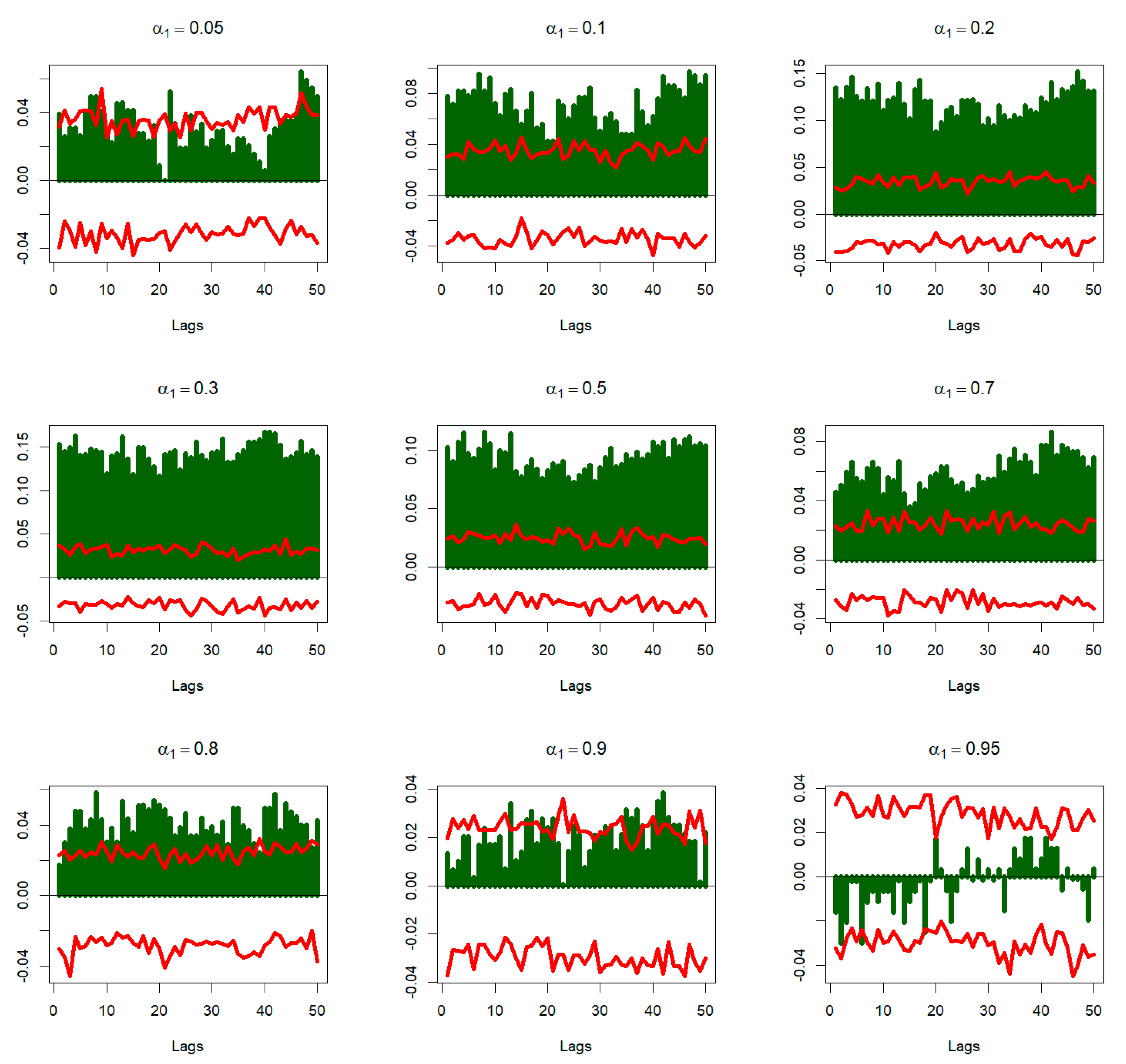
Figure 1, Figure 2 and Figure 3 depict the cross-quantilograms ${\rho }_{\tau }^{*}{ }^{ }\left(k\right)$, which detect the directional predictability of the realized stock-bond correlation jumps from time varying risk aversion (TVRA) by estimating the lead-lag correlations contemporarily at different lags and at various quantiles of the risk aversion, i.e., for the ${\alpha }_2=0.1$, ${\alpha }_2=0.5$, and ${\alpha }_2=0.9$ quantiles, which correspond to market states when risk aversion is at its low, median, and high levels, respectively.

Given that correlation jumps and risk aversion series are at daily frequency in our empirical application, a large number of lags is selected, i.e., $k=50$, and the lead/lag correlations are estimated for each lag. The latter corresponds to 50 days, i.e., slightly less than 2 months, in order to account for practical applications to portfolio allocation decisions, as daily rebalancing of investment portfolios would not make much sense due to transaction costs. The (green) bars in the graphs depict the estimated ${\rho }_{\tau }^{*}{}^{ }\left(k\right)$ values, while the red lines depict the $95\%$ bootstrap confidence intervals obtained from $1000$ bootstrap iterations. For positive ${\rho }_{\tau }^{*}{}^{ }\left(k\right)$ values, a bar above the red line leads to the rejection of the null hypothesis $H_0: {\widehat{q}}_a\left(k\right)=0$ at a $5\%$ significance level. For negative ${\rho }_{\tau }^{*}{}^{}\left(k\right)$ values, a bar below the red line leads to the rejection of the null hypothesis $H_0: {\widehat{q}}_a\left(k\right)=0$ at a $5\%$ significance level.

Figure 1 represents the case in which the TVRAs are in their low quantile (${\alpha }_2$ = 0.1), thus capturing the market state in which investors have greater risk appetite. We observe a weak level of positive dependency for some lags between the TVRA and $RCJ$, when $RCJ$ are in their low quantile (${\alpha }_1$ = 0.1). The ${\rho }_{\tau }^{*}{}^{ }\left(k\right)$ are estimated to be positive and significantly different from zero only for few lags. This means that when TVRA is very low, i.e., investors have greater appetite for risk taking, it is unlikely to have high levels of $RCJ$ both in medium-term and long-term periods. Thus, we can argue that periods of greater risk appetite or speculative tendencies are not necessarily associated with longer term jumps in correlations between stock and bond market returns. However, when $RCJ$ are in their median quantile (${\alpha }_1$ = 0.5), we observe a positive dependency between TVRA and $RCJ$ for all considered lags, suggesting that low level of risk aversion captures predictive information on typical occurrences of correlations jumps represented by median levels of $RCJ$. At the other extreme, that is when $RCJ$ are in their high quantile (${\alpha }_1$ = 0.9), we find a positive dependency between TVRA and $RCJ$ after some lags. The ${\rho }_{\tau }^{*}{}^{ }\left(k\right)$ are positive and significantly different from zero after the first several lags for a lower number of lags, compared to the previous case. This suggests that when TVRA is very low, it is more likely to have high levels of $RCJ$. In economic terms, the findings suggest that greater speculative tendencies among investors can predict immediate correlation jumps, possibly due to correlated trades in stock and bond markets as investors allocate funds in and out of these assets, thus establishing a predictive relation between risk aversion and jumps in correlations. Accordingly, one can argue that risk aversion has an asymmetric impact on correlation patterns such that speculative and hedging tendencies among investors can contribute to heterogeneity in correlation patterns.

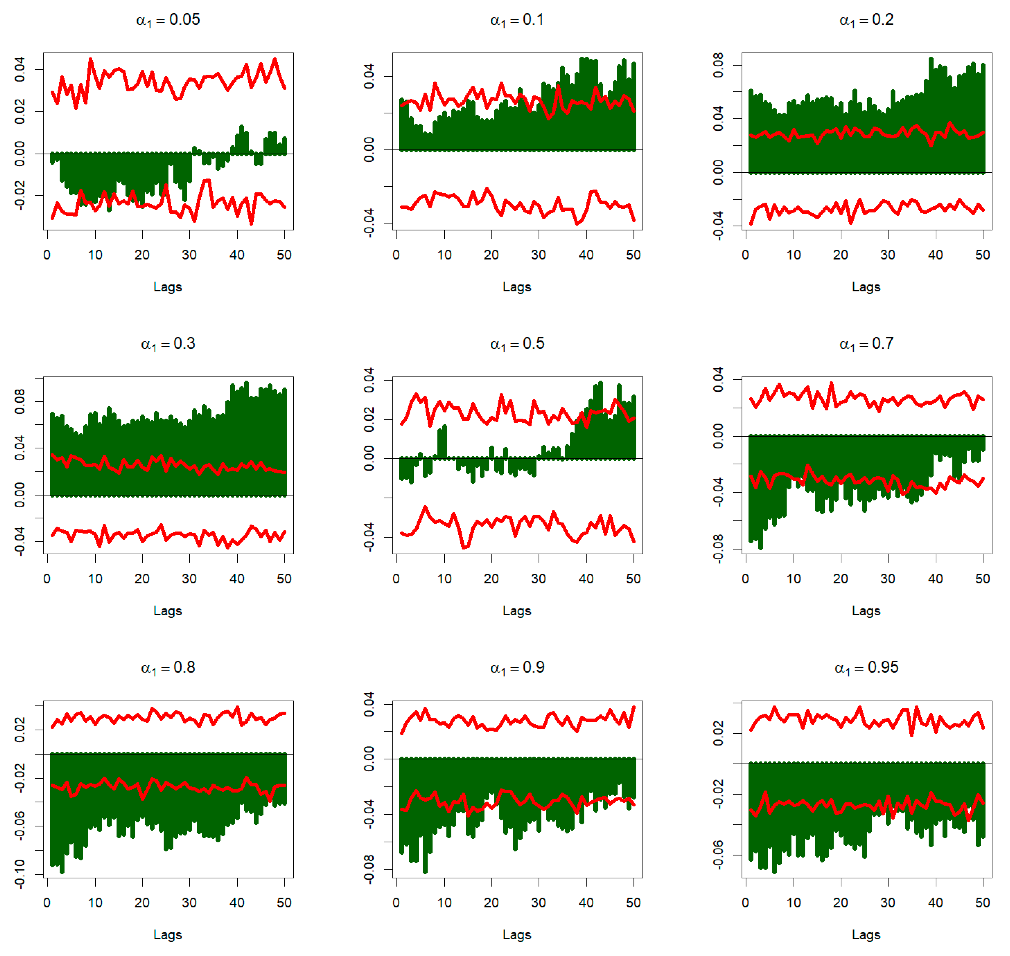
Figure 2 represents the case in which the TVRA is in its median quantile (${\alpha }_2$ = 0.5), corresponding to typical market states as far as investor risk attitudes are concerned. We observe a weak level of negative dependency after some lags between the TVRA and $RCJ$, when $RCJ$ are in their low quantile (${\alpha }_1$ = 0.1). The estimated ${\rho }_{\tau }^{*}{}^{ }\left(k\right)$ values are negative and significantly different from zero only for few lags. The latter means that when TVRA is very low, it is unlikely to have low levels of $RCJ$ both in medium-term and long-term periods. At the same time, when $RCJ$ are in their median quantile (${\alpha }_1$ = 0.5), we report a positive dependency between TVRA and $RCJ$ for a few lags only in the long-term period. When $RCJ$ are in their high quantile (${\alpha }_1$ = 0.9), however, a negative dependency is observed between TVRA and $RCJ$ for the immediate short-term lags. The ${\rho }_{\tau }^{*}{}^{ }\left(k\right)$ are found to be significantly different from zero after the first several lags for a greater number of lags, compared to the previous case. Therefore, we conclude that when TVRA is in its median levels, it is unlikely to have high levels of $RCJ$ in both the short-and long-term periods. This suggests that typical risk aversion values do not necessarily capture predictive information over correlation jump dynamics, implying a regime specific predictability relation between investors’ risk preferences and correlation patterns.

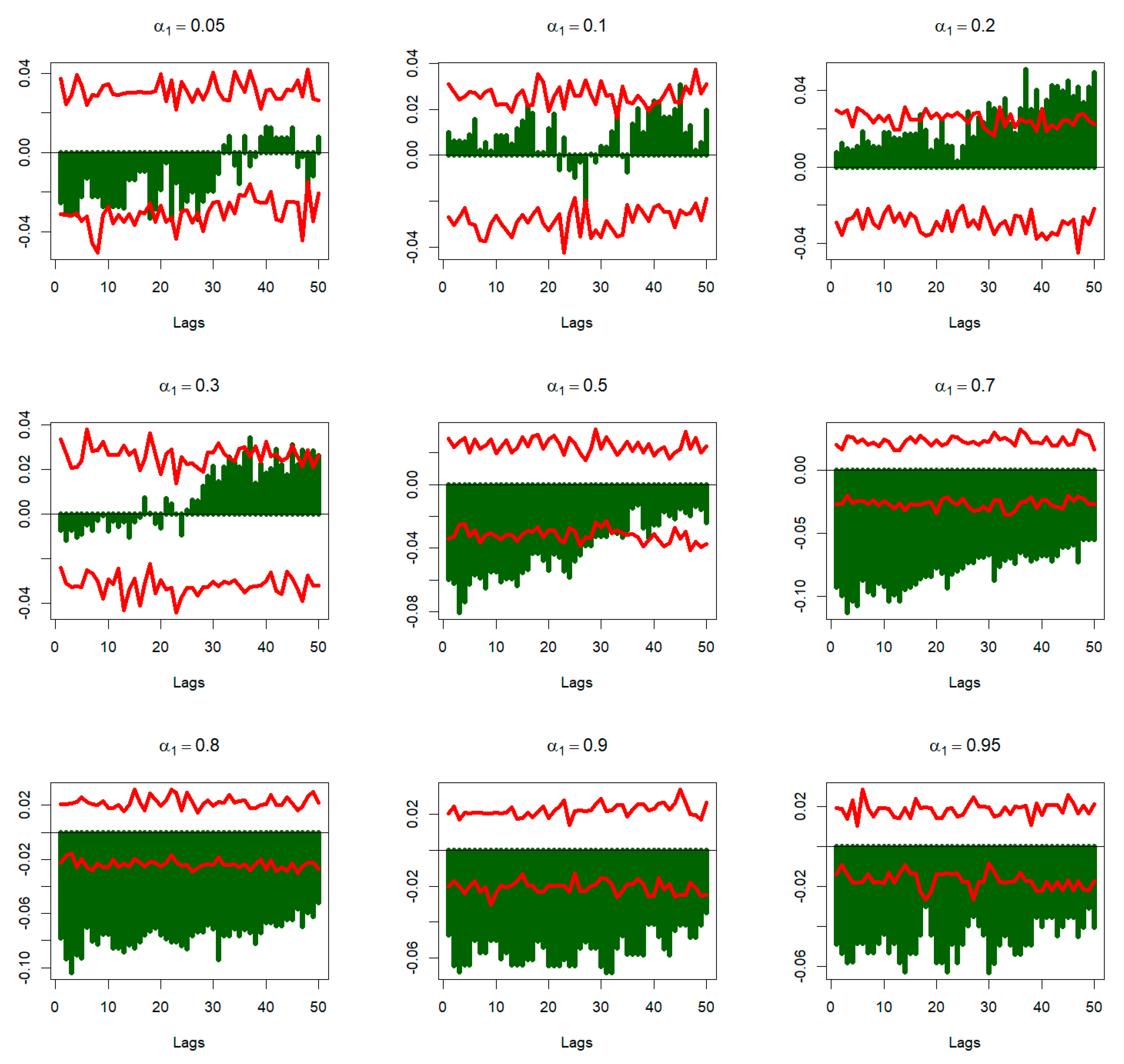
Finally, Figure 3 represents the case in which the TVRA is in its extreme high quantile (${\alpha }_2$ = 0.9), capturing market states in which investors have greater hedging tendencies. We observe a weak level of positive dependency after some lags between the TVRA and $RCJ$, when $RCJ$ are in their low quantile (${\alpha }_1$ = 0.1). The estimated ${\rho }_{\tau }^{*}{}^{ }\left(k\right)$ values are positive and significantly different from zero only for few lags, implying that when TVRA is very high, it is likely to have low levels of $RCJ$ both in short- and long-term periods. When $RCJ$ are in their median quantile (${\alpha }_1$ = 0.5), however, we find a strong positive dependency between TVRA and $RCJ$ for all lags considered. At the other extreme, when $RCJ$ are in their high quantile (${\alpha }_1$ = 0.9), we find a weak positive dependency between TVRA and $RCJ$ after some lags. The ${\rho }_{\tau }^{*}{}^{ }\left(k\right)$ are found to be positive and significantly different from zero after the first few lags. Therefore, we conclude that when TVRA is very high, it is not likely to have high levels of $RCJ$ in both the short- and long-term periods. From an economic perspective, the latter indicates that greater hedging tendencies are not necessarily associated with future occurrences of jumps in correlation patterns, as investors would be less likely to increase their allocations to equity positions in such market states.

Overall, the inferences obtained from Figure 1, Figure 2 and Figure 3 point to a regime specific predictive relation between behavioral factors and correlation dynamics such that greater speculative tendencies, i.e., TVRA at extreme low levels, are more likely to be associated with future occurrences of jumps in stock-bond market correlations, while market states during which hedging tendencies dominate do not necessarily capture predictive information regarding future occurrences of correlation jumps. For investment allocation and diversification applications, the results suggest that, failing to take into account the level of risk aversion in financial markets can lead to under-diversified portfolio positions during periods when speculative tendencies are high. This is indeed an important consideration, as greater risk taking can lead to excess volatility in investment returns, and, based on our findings, taking into account the level of risk appetite can help improve the effectiveness of diversification schemes.

4. Conclusions

In this paper, the predictive role of time-varying risk aversion over correlation dynamics in stock and bond returns is examined. The empirical analysis reveals an asymmetric relation between realized stock-bond correlation jumps and time-varying risk aversion, detecting a heterogeneous dependence pattern across different quantiles and lag orders. Specifically, a strong level of negative dependency between time varying risk aversion and the realized stock-bond correlation jumps is observed when the latter is at its medium levels. Said dependencies tend to be stronger for large lags, i.e., for lags over 30 days. When risk aversion is at its median levels, reflective of typical market states for investor behavior, very strong negative dependencies in almost all lags at all but the very low realized stock-bond correlation jumps indicator’s quantiles are documented. Said negative dependencies are stronger for earlier lags, reflecting short term effects, while for longer lags, no dependency is observed. Finally, when the varying risk aversion is at its high levels, strong negative dependencies are observed at almost all levels of the realized stock-bond correlation jumps indicator, and for most lags. At the low realized stock-bond correlation jumps quantiles, statistically significant dependencies are mainly observed for very large lags, all of which are negative.

The findings establish a regime-dependent predictive relationship between behavioral factors and correlation jumps in financial markets, which can be utilized to avoid under-diversification in extreme market conditions when diversification is needed the most. These findings have important implications for policy makers as they allow us to better understand changes in the correlation between stock and bond market returns as such changes reflect important variations in macroeconomic conditions and/or investors’ risk preferences. However, there are some limitations, mainly concerning the period selection due to data availability, as well as the fact that we only focus on the US market. For future research, it would be interesting to extend the scope of our study to alternative investments including commodities or crypto currencies, as one would expect the time-variation in risk appetite to have stronger effects in these relatively riskier asset classes, and to evaluate the out-of-sample predictive power of TVRA on correlation dynamics in those markets.

References

- Longin, F.; Solnik, B. Extreme correlation of international equity markets. J. Financ. 2001, 56, 649–676. [Google Scholar] [CrossRef]
- Goetzmann, W.N.; Kumar, A. Equity portfolio diversification. Rev. Financ. 2008, 12, 433–463. [Google Scholar] [CrossRef] [Green Version]
- Levy, H.; Sarnat, M. International diversification of investment portfolios. Am. Econ. Rev. 1970, 60, 668–675. [Google Scholar]
- Yang, J.; Zhou, Y.; Wang, Z. The stock–bond correlation and macroeconomic conditions: One and a half centuries of evidence. J. Bank. Financ. 2009, 33, 670–680. [Google Scholar] [CrossRef]
- Scruggs, J.T.; Glabadanidis, P. Risk premia and the dynamic covariance between stock and bond returns. J. Financ. Quant. Anal. 2003, 38, 295–316. [Google Scholar] [CrossRef]
- Connolly, R.; Stivers, C.; Sun, L. Stock market uncertainty and the stock–bond return relation. J. Financ. Quant. Anal. 2005, 40, 161–194. [Google Scholar] [CrossRef] [Green Version]
- Connolly, R.; Stivers, C.; Sun, L. Commonality in the time variation of stock–bond and stock–stock return co-movements. J. Financ. Mark. 2007, 10, 192–218. [Google Scholar] [CrossRef]
- Kim, S.; Moshirian, F.; Wu, E. Evolution of international stock and bond market integration: Influence of the European Monetary Union. J. Bank. Financ. 2006, 30, 1507–1534. [Google Scholar] [CrossRef] [Green Version]
- Li, L. Macroeconomic Factors and the Correlation of Stock and Bond Returns; Working Paper; Yale University: New Haven, CT, USA, 2002. [Google Scholar]
- d’Addona, S.; Kind, A.H. International stock–bond correlations in a simple affine asset pricing model. J. Bank. Financ. 2006, 30, 2747–2765. [Google Scholar] [CrossRef]
- Boyd, J.H.; Jagannathan, R.; Hu, J. The stock market’s reaction to unemployment news: Why bad news is usually good for stocks. J. Financ. 2005, 60, 649–672. [Google Scholar] [CrossRef]
- Andersen, T.G.; Bollerslev, T.; Diebold, F.X.; Vega, C. Real-time price discovery in stock, bond and foreign exchange markets. J. Int. Econ. 2007, 73, 251–277. [Google Scholar] [CrossRef] [Green Version]
- Ilmanen, A. Stock–bond correlations. J. Fixed Income 2003, 12, 55–66. [Google Scholar] [CrossRef] [Green Version]
- Jensen, G.R.; Mercer, J.M. New evidence on optimal asset allocation. Financ. Rev. 2003, 38, 435–454. [Google Scholar] [CrossRef]
- Huang, D.; Jiang, F.; Tu, J.; Zhou, G. Investor Sentiment Aligned: A Powerful Predictor of Stock Returns. Rev. Financ. Stud. 2015, 28, 791–837. [Google Scholar] [CrossRef]
- Baker, M.; Wurgler, J. Investor sentiment and the cross-section of stock returns. J. Financ. 2006, 61, 1645–1680. [Google Scholar] [CrossRef] [Green Version]
- Bams, D.; Honarvar, I.; Lehnert, T. Risk Aversion, Sentiment and the Cross-Section of Stock Returns; Working Paper Limburg Institute of Financial Economics (LIFE); Maastricht University: Maastricht, The Netherlands, 2017. [Google Scholar]
- Demirer, R.; Gkillas, K.; Gupta, R.; Pierdzioch, C. Time-varying risk aversion and realized gold volatility. N. Am. J. Econ. Financ. 2019, 50, 101048. [Google Scholar] [CrossRef] [Green Version]
- Xu, N.R. Global Risk Aversion and International Return Comovements. Available online: https://papers.ssrn.com/sol3/papers.cfm?abstract_id=3174176 (accessed on 11 September 2020).
- Demirer, R.; Omay, T.; Yuksel, A. Global Risk Aversion and Emerging Market Correlations. Econ. Lett. 2018, 173, 118–121. [Google Scholar] [CrossRef]
- Gkillas, K.; Longin, F. Is Bitcoin the New Digital Gold? Evidence from Extreme Price Movements in Financial Markets. Available online: https://papers.ssrn.com/sol3/papers.cfm?abstract_id=3245571 (accessed on 11 September 2020).
- Guiso, L.; Sapienza, P.; Zingales, L. Time varying risk aversion. J. Financ. Econ. 2018, 128, 403–421. [Google Scholar] [CrossRef] [Green Version]
- Bekaert, G.; Engstrom, E.C.; Xu, N.R. The Time Variation in Risk Appetite and Uncertainty. Available online: https://www.nber.org/papers/w25673 (accessed on 11 September 2020).
- Barndorff-Nielsen, O.E.; Shephard, N. Econometric analysis of realized covariation: High frequency based covariance, regression, and correlation in financial economics. Econometrica 2004, 72, 885–925. [Google Scholar] [CrossRef]
- Christensen, K.; Oomen, R.; Podolskij, M. Realised quantile-based estimation of the integrated variance. J. Econom. 2010, 159, 74–98. [Google Scholar] [CrossRef] [Green Version]
- Todorova, N. Volatility estimators based on daily price ranges versus the realized range. Appl. Financ. Econ. 2012, 22, 215–229. [Google Scholar] [CrossRef]
- Gkillas, K.; Vortelinos, D.; Saha, S. The properties of realized volatility and realized correlation: Evidence from the Indian stock market. Phys. A Stat. Mech. Its Appl. 2018, 492, 343–359. [Google Scholar] [CrossRef]
- Corsi, F.; Pirino, D.; Reno, R. Threshold bipower variation and the impact of jumps on volatility forecasting. J. Econom. 2010, 159, 276–288. [Google Scholar] [CrossRef] [Green Version]
- Andersen, T.G.; Dobrev, D.; Schaumburg, E. Jump-robust volatility estimation using nearest neighbor truncation. J. Econom. 2012, 169, 75–93. [Google Scholar] [CrossRef] [Green Version]
- Heejoon, H.; Linton, O.; Oka, T.; Whang, Y.J. The Cross-Quantilogram: Measuring Quantile Dependence and Testing Directional Predictability between Time Series. J. Econom. 2016, 193, 251–270. [Google Scholar]
- Linton, O.; Whang, Y.J. The Quantilogram: With an Application to Evaluating Directional Predictability. J. Econom. 2017, 141, 250–282. [Google Scholar] [CrossRef]
- Fengler, M.R.; Gisler, K.I. A variance spillover analysis without covariances: What do we miss? J. Int. Money Financ. 2015, 51, 174–195. [Google Scholar] [CrossRef] [Green Version]
- Andersen, T.G.; Bollerslev, T.; Diebold, F.X.; Labys, P. Modelling and forecasting realized volatility. Econometrica 2003, 71, 579–625. [Google Scholar] [CrossRef] [Green Version]
- Politis, D.; Romano, J.P. The stationary Bootstrap. J. Am. Stat. Assoc. 1994, 89, 1303–1313. [Google Scholar] [CrossRef]
- Jacod, J.; Shiryaev, A.N. Limit Theorems for Stochastic Processes; Springer: Berlin/Heidelberg, Germany, 2003; ISBN 978-3-662-05265-5. [Google Scholar]
Figure 1.
Sample cross-quantilograms for the low levels of TVRAs, i.e., for . Note: This figure depicts the sample cross-quantilograms to detect directional predictability from time-varying risk aversion measure (TVRA) to realized correlation jumps , by estimating the lead-lag correlations contemporarily at different lags and quantiles. As for , six quantiles are considered, in which As for TVRA, three quantiles are considered, in which corresponding to periods in which the TVRA is in its low levels. Bar graphs depict the , while the red lines depict the bootstrap confidence intervals for bootstrap iterations. For positive (negative) values of the , a bar above (below) the red line leads to a rejection of the null hypothesis at a significance level.
Figure 2.
Sample cross-quantilograms for the median levels of TVRAs, i.e., for . Note: This figure depicts the sample cross-quantilograms to detect directional predictability from time-varying risk aversion measure (TVRA) to realized correlation jumps , by estimating the lead-lag correlations contemporarily at different lags and quantiles. As for , six quantiles are considered, in which As for TVRA, three quantiles are considered, in which corresponding to periods in which the TVRA is in its median levels. Bar graphs depict the , while the red lines depict the bootstrap confidence intervals for bootstrap iterations. For positive (negative) values of the , a bar above (below) the red line leads to a rejection of the null hypothesis at a significance level.
Figure 3.
Sample cross-quantilograms for the high levels of TVRAs, i.e., for . Note: This figure depicts the sample cross-quantilograms to detect directional predictability from time-varying risk aversion measure (TVRA) to realized correlation jumps , by estimating the lead-lag correlations contemporarily at different lags and quantiles. As for , six quantiles are considered, in which As for TVRA, three quantiles are considered, in which corresponding to periods in which the TVRA is in its high levels. Bar graphs depict the , while the red lines depict the bootstrap confidence intervals for bootstrap iterations. For positive (negative) values of the , a bar above (below) the red line leads to a rejection of the null hypothesis at a significance level.
Publisher’s Note: MDPI stays neutral with regard to jurisdictional claims in published maps and institutional affiliations. |
© 2020 by the authors. Licensee MDPI, Basel, Switzerland. This article is an open access article distributed under the terms and conditions of the Creative Commons Attribution (CC BY) license (http://creativecommons.org/licenses/by/4.0/).
Share and Cite
MDPI and ACS Style
Demirer, R.; Gkillas, K.; Kountzakis, C.; Mavragani, A. Risk Appetite and Jumps in Realized Correlation. Mathematics 2020, 8, 2255. https://0-doi-org.brum.beds.ac.uk/10.3390/math8122255
AMA Style
Demirer R, Gkillas K, Kountzakis C, Mavragani A. Risk Appetite and Jumps in Realized Correlation. Mathematics. 2020; 8(12):2255. https://0-doi-org.brum.beds.ac.uk/10.3390/math8122255
Chicago/Turabian StyleDemirer, Riza, Konstantinos Gkillas, Christos Kountzakis, and Amaryllis Mavragani. 2020. "Risk Appetite and Jumps in Realized Correlation" Mathematics 8, no. 12: 2255. https://0-doi-org.brum.beds.ac.uk/10.3390/math8122255
Note that from the first issue of 2016, this journal uses article numbers instead of page numbers. See further details here.