Delay Cournot Duopoly Game with Gradient Adjustment: Berezowski Transition from a Discrete Model to a Continuous Model

Abstract

This paper investigates the asymptotical behavior of the equilibrium of linear classical duopolies by reconsidering the two-delay model with two different positive delays. In a two-dimensional analysis, the stability switching curves were first analytically determined. Numerical studies verified and illustrated the theoretical results. In the sensitivity analysis it was demonstrated that the inertia coefficient has a twofold effect: enlarges the stability region as well as simplifies the complicated dynamics with period-halving cascade. In contrary, the adjustment speed contracts the stability region and complicates simple dynamics with period-doubling bifurcation. In addition, for various values of ${\tau }_1$ and ${\tau }_2,$ a wide variety of dynamics appears ranging from simple cycle via a Hopf bifurcation to chaotic oscillations.

1. Introduction

The earliest studies on oligopoly theory focused on the existence and uniqueness of the equilibrium. If the firms are in an equilibrium state, then the common interest of the firms is to keep this state. However, in a disequilibrium situation, the firms start to adjust their output levels in order to gain as much profit as possible. So a dynamic process develops. There are many different versions of such models. First is the selection of time scales. The reason for using discrete time scales is based on the fact that the firms need to use time-to-build technology, so they can act only after certain delays, which can be used as time steps. The mathematical methodology to deal with the resulting difference equations is well established. Trading takes place repeatedly almost instantaneously in many cases in which the choice of continuous time scales is more appropriate. A bridge between discrete and continuous time models is the selection of continuous time scales and the introduction of discrete delays. This makes sense economically, since collecting information about the competitors, determining best decision and its implementation need time. If the delay is known, then discrete delays are used, and if they are uncertain, then they are considered random and, therefore, continuously distributed delays are assumed. Several model variants were developed based on the type of the adjustment process, which is based on how the firms assess the actions of the competitors. Static, adaptive, extrapolative expectations or sequential adjustment processes are mostly assumed. Another choice is between best response and gradient dynamics. In the linear cases, they are mathematically equivalent, the only difference is between the speeds of adjustments. In the earliest studies, linear models were assumed, which were easy to examine and local stability implied global stability.

A summary of the results up to the mid 1970s can be found in [1] and their multi-product generalizations are discussed in [2]. If the model is nonlinear, then there are several ways to examine stability. The Lyapunov function method can be used to show marginal stability, and local and global asymptotical stability. Its foundation can be found in almost any textbook on ordinary differential equations, such as [3]. In the discrete case, the critical curve method is often used to detect the long-term behavior of the firms [4]. The most common approach is local linearization around the equilibrium. The linearized equations are the same as those of linear oligopolies and their asymptotical stability implies local asymptotical stability in the nonlinear models. [5] offered a comprehensive summary of stability analysis of nonlinear oligopolies. If discrete time scales are selected, then the delays are integers, so the delay equations are equivalent with higher order equations without delays. In the case of continuous time scales, differential-difference equations describe the dynamic processes. Ref [6] contains the most important properties of such models.

In the economic literature, the classical Cournot model is most frequently examined with gradient adjustments. An example of selecting continuously distributed delays is given for example, in [7]. The mathematical methods for analyzing the stability of models with two and three delays are developed in [8,9]. Based on mathematical developments, many studies examined different classes of dynamic economic models with delays such as [10,11,12,13] among others. Different versions of delay oligopolies are discussed with discrete and continuous time scales in [14], where the mathematical methodology is also presented in detail. A new development was the introduction of the inertia coefficient in modeling difficulties in adjusting production over time. This idea was known earlier from physics (e.g., [15]) and was first introduced into economics by [16]. An important further step was given by [11] by introducing an interesting version of transforming discrete time oligopolies to continuous time models with two discrete delays and gave stability analysis in several cases. This paper is based on Gori’s model considering two positive different delays. In a two-dimensional analysis, the stability switching curves are analytically determined and verified with numerical studies in which the effects of the inertia coefficient and the adjustment speeds on the asymptotic behavior of the equilibrium are also demonstrated.

The paper develops as follows. Section 2 introduces the basic model. The stability switching curves are analytically determined in Section 3. Numerical studies of Section 4 verify and illustrate the theoretical results and sensitivity analysis is detailed with respect to the inertia coefficient and the speeds of adjustments. Concluding remarks and further research directions are outlined in the final section.

2. Model

There are two firms in a market. Firm i produces output $x_i$ with the production marginal cost $c_i$.A normalized linear price function is

$$p=1-(x_1+x_2).$$

The profit of firm i is

$${\pi }_i=\left(1-x_1-x_2\right)x_i-c_i{x}_i.$$

Assumption A1.

$c_i=c$ for $i=1,2$ and $0<c<1.$

Each firm determines its output to maximize its profit. The first-order conditions for profit maximization are

$$\frac{\partial {\pi }_i}{\partial x_i}=1-c-2x_i-x_j=0\mathrm{for}i,j=1,2\mathrm{and}i\ne j$$

and the second-order conditions are confirmed. Solving the first-order conditions gives the Cournot equilibrium outputs,

$$x_i^{*}=x_j^{*}=x^{*}=\frac{1-c}{3}.$$

In the output adjustment process, [17] adopt the gradient method in a discrete-time framework,

$$x_i(t+1)=x_i\left(t\right)+\alpha x_i\left(t\right)\frac{\partial {\pi }_i\left(t\right)}{\partial x_i\left(t\right)}$$

(1)

where $\alpha$ is a positive adjustment coefficient and reveals that the dynamic system can generate various dynamics including chaotic behavior. To re-examine the gradient dynamics in a continuous-time framework, based on [11,15] constructed the following forms of the dynamic equations with distinct time delays,

$$\begin{array}{c}{\dot{x}}_1\left(t\right)=\frac{-x_1\left(t\right)+x_1(t-{\tau }_1)+\alpha x_1(t-{\tau }_1)\left[1-c-2x_1(t-{\tau }_1)-x_2(t-{\tau }_1)\right]}{{\sigma }_1},\hfill \\ \\ {\dot{x}}_2\left(t\right)=\frac{-x_2\left(t\right)+x_2(t-{\tau }_2)+\alpha x_2(t-{\tau }_2)\left[1-c-x_1(t-{\tau }_2)-2x_2(t-{\tau }_2)\right]}{{\sigma }_2}\hfill \end{array}$$

(2)

where ${\sigma }_i>0$ weights the inertia in the production process of firm $i$ and $\left({\tau }_1,{\tau }_2\right)\ge 0$ are two parameters that capture time delays. Ref. [11] considers the following cases,

$$\begin{array}{c}\left(1\right){\tau }_1={\tau }_2=\tau ,{\sigma }_1={\sigma }_2\mathrm{and}{x}_1\left(t\right)=x_2\left(t\right)\mathrm{for}t\in [-\tau ,0),\hfill \\ \left(2\right){\tau }_1=0\mathrm{and}{\tau }_2>0,\hfill \\ \left(3\right){\tau }_1>0\mathrm{and}{\tau }_2\mathrm{is}\mathrm{fixed}\mathrm{in}\mathrm{its}\mathrm{stable}\mathrm{interval},[0,{\tau }_{20}),\hfill \\ \left(4\right){\tau }_1={\tau }_2.\hfill \end{array}$$

All these cases lead to single-delay systems. We complement their study by considering both delays as variables and perform a bivariable analysis for

$${\tau }_1>0,{\tau }_2>0\mathrm{and}{\tau }_1\ne {\tau }_2.$$

3. Stability Switching Curves

To find out information about the stability of the Cournot point, we linearize the dynamic system around it and take its homogeneous version,

$$\begin{array}{c}{\dot{x}}_1\left(t\right)={\displaystyle \frac{-x_1\left(t\right)+x_1(t-{\tau }_1)+\alpha x^{*}\left[-2x_1(t-{\tau }_1)-x_2(t-{\tau }_1)\right]}{{\sigma }_1}},\hfill \\ \\ {\dot{x}}_2\left(t\right)={\displaystyle \frac{-x_2\left(t\right)+x_2(t-{\tau }_2)+\alpha x^{*}\left[-x_1(t-{\tau }_2)-2x_2(t-{\tau }_2)\right]}{{\sigma }_2}}.\hfill \end{array}$$

(3)

Substituting exponential solutions $x_i\left(t\right)=e^{\lambda t}{u}_i$, these equations give a homogeneous system of $u_1$ and $u_2$. Nontrivial solution exists if its determinant is zero, leading to the the characteristic equation,

$$det\left(\begin{array}{cc}\lambda +{\displaystyle \frac{1}{{\sigma }_1}}\left(1-e^{-\lambda {\tau }_1}+2\alpha x^{*}{e}^{-\lambda {\tau }_1}\right)& {\displaystyle \frac{\alpha x^{*}}{{\sigma }_1}}{e}^{-\lambda {\tau }_1}\\ {\displaystyle \frac{\alpha x^{*}}{{\sigma }_2}}{e}^{-\lambda {\tau }_2}& \lambda +{\displaystyle \frac{1}{{\sigma }_2}}\left(1-e^{-\lambda {\tau }_2}+2\alpha x^{*}{e}^{-\lambda {\tau }_2}\right)\end{array}\right)=0.$$

As a benchmark, we examine the no-delay case of ${\tau }_1={\tau }_2=0$ in which the characteristic equation reads

$${\lambda }^2+\frac{2\alpha x^e\left({\sigma }_1+{\sigma }_2\right)}{{\sigma }_1{\sigma }_2}\lambda +\frac{3{\left(\alpha x^e\right)}^2}{{\sigma }_1{\sigma }_2}=0.$$

The discriminant of this equation is positive, so the positive coefficients imply that the characteristic roots are real and negative, leading to the locally asymptotically stability of Cournot point. (see Lemma 3 of [11] in which this stability result already has been shown.) Since it is verified that $\lambda =0$ does not solve the characteristic equation with positive delays, the stability of the Cournot point depends on the locations of the roots of the characteristic equation in the complex plane. To proceed, we first expand the determinant and simplify the characteristic equation as follows:

$$\begin{array}{c}\left(1+{\sigma }_1\lambda \right)\left(1+{\sigma }_2\lambda \right)-\left(1-2\alpha x^{*}\right)\left(1+{\sigma }_2\lambda \right)e^{-\lambda {\tau }_1}\\ -\left(1-2\alpha x^{*}\right)\left(1+{\sigma }_1\lambda \right)e^{-\lambda {\tau }_2}+\left(1-\alpha x^{*}\right)\left(1-3\alpha x^{*}\right)e^{-\lambda \left({\tau }_1+{\tau }_2\right)}=0.\end{array}$$

We then assume $\lambda =i\omega$ with $\omega >0$ and substitute it into the above equation to yield

$$\left(P_0\left(i\omega \right)+P_1\left(i\omega \right)e^{-i\omega {\tau }_1}\right)+\left(P_2\left(i\omega \right)+P_3\left(i\omega \right)e^{-i\omega {\tau }_1}\right)e^{-i\omega {\tau }_2}=0.$$

(4)

where

$$\begin{array}{c}{P}_0\left(i\omega \right)=\left(1+i{\sigma }_1\omega \right)\left(1+i{\sigma }_2\omega \right),\hfill \\ P_1\left(i\omega \right)=-\left(1-2\alpha x^{*}\right)\left(1+i{\sigma }_2\omega \right),\hfill \\ P_2\left(i\omega \right)=-\left(1-2\alpha x^{*}\right)\left(1+i{\sigma }_1\omega \right),\hfill \\ P_3\left(i\omega \right)=\left(1-\alpha x^{*}\right)\left(1-3\alpha x^{*}\right).\hfill \end{array}$$

(5)

Applying the method developed by [14] (Appendix A) that is based on [9], we derive the set of point (${\tau }_1,{\tau }_2$) for which the delay system (2) has purely complex roots.

Lemma 1.

The characteristic Equation (4) can be written as

$${\left|P_0\right|}^2+{\left|P_1\right|}^2-{\left|P_2\right|}^2-{\left|P_3\right|}^2=2A_1\left(\omega \right)cos\omega {\tau }_1-2B_1\left(\omega \right)sin\omega {\tau }_1$$

where

$$A_1\left(\omega \right)=A\mathrm{and}{B}_1\left(\omega \right)={\sigma }_1\omega A$$

with

$$A={\displaystyle \frac{\left[3-2\alpha (1-c)\right]\left\{3{\sigma }_2^2{\omega }^2-\alpha (1-c)\left[\alpha (1-c)-4\right]\right\}}{9}}.$$

(6)

Proof. 

See Appendix A. □

Concerning the sign of A defined in Lemma 1, we have the following results.

Proposition 1.

The sign of A is determined in the following way.

$$\begin{array}{c}if\alpha (1-c)<3/2,thenA>0,\hfill \\ if\alpha (1-c)=3/2,thenA=0\hfill \\ if3/2<\alpha (1-c)\le 4,thenA<0.\hfill \end{array}$$

Proof. 

Proof is clear from (6),the definition of A. □

The definition of A can be rewritten as

$$A={\displaystyle \frac{{\sigma }_2^2\left[3-2\alpha (1-c)\right]}{3}}\left(\omega +\overline{\omega }\right)\left(\omega -\overline{\omega }\right)$$

(7)

where

$$\overline{\omega }=\frac{\sqrt{\alpha (1-c)\left[\alpha (1-c)-4\right]}}{\sqrt{3}{\sigma }_2}\left\{\begin{array}{c}=0\mathrm{if}\alpha \left(1-c\right)=4,\hfill \\ >0\mathrm{if}\alpha \left(1-c\right)>4,\hfill \\ \mathrm{complex}\mathrm{if}\alpha \left(1-c\right)<4.\hfill \end{array}\right.$$

(8)

Then we have

Proposition 2.

If $\alpha (1-c)>4$,then $A>0$ as $\omega <\overline{\omega },A=0$ as $\omega =\overline{\omega }$ and $A<0$ as $\omega >\overline{\omega }.$

Proof. 

Proof is clear form (7), a different form defining A. □

3.1. $A_1{\left(\omega \right)}^2+B_1{\left(\omega \right)}^2>0$

In this subsection, A is nonzero, so $\alpha (1-c)$ differs from $3/2$. For the sake of analytical simplicity, we impose the following:

• Assumption 2. $\alpha (1-c)\le 4.$

The case of $\alpha (1-c)>4$ will be examined at the end of this section. For analytical simplicity, we impose the following:

• Assumption 3. ${\sigma }_1={\sigma }_2=\sigma$.

First, we determine the feasible range of $\omega$. Assumptions 1 and 3 together imply that the firms are identical.

Lemma 2.

Under Assumptions 1, 2 and 3, the characteristic Equation (4) can be written as

$${\left|P_0\right|}^2+{\left|P_1\right|}^2-{\left|P_2\right|}^2-{\left|P_3\right|}^2=2\sqrt{A_1{\left(\omega \right)}^2+B_1{\left(\omega \right)}^2}cos\left[{\varphi }_1\left(\omega \right)+\omega {\tau }_1\right]$$

(9)

with

$${\varphi }_1\left(\omega \right)=arg\left[P_2{\overline{P}}_3-P_0{\overline{P}}_1\right].$$

Proof. 

See the Appendix A. □

To satisfy the transformed characteristic Equation (9) defined in Lemma 2, we need

$$\left|\frac{{\left|P_0\right|}^2+{\left|P_1\right|}^2-{\left|P_2\right|}^2-{\left|P_3\right|}^2}{2\sqrt{A_1{\left(\omega \right)}^2+B_1{\left(\omega \right)}^2}}\right|\le 1.$$

(10)

Define a function,

$$F\left(\omega \right)={\left({\left|P_0\right|}^2+{\left|P_1\right|}^2-{\left|P_2\right|}^2-{\left|P_3\right|}^2\right)}^2-4\left(A_1{\left(\omega \right)}^2+B_1{\left(\omega \right)}^2\right).$$

An $\omega$ value is feasible if and only if $F\left(\omega \right)\le 0$. With substituting $P_k\left(i\omega \right)$ for $k=0,1,2,3$ in (5), $A_1\left(\omega \right)$ and $B_1\left(\omega \right)$ into the right hand side of $F\left(\omega \right),$ and defining $x={\omega }^2,$ we can rewrite $F\left(\omega \right)$ as

$$f\left(x\right)=a_4{x}^4+a_3{x}^3+a_2{x}^2+a_{1}x+a_0$$

where

$$\begin{array}{c}{a}_4={\sigma }^8,\hfill \\ a_3=-{\displaystyle \frac{16\alpha (1-c)\left[3-\alpha (1-c)\right]}{9}}{\sigma }^6,\hfill \\ a_2={\displaystyle \frac{2{\alpha }^2{(1-c)}^2\left[138-88\alpha (1-c)+13{\alpha }^2{(1-c)}^2\right]}{27}}{\sigma }^4,\hfill \\ a_1=-{\displaystyle \frac{8{\alpha }^3{(1-c)}^3\left[4-\alpha (1-c)\right]\left[7\left(3-2\alpha (1-c)\right)+2{\alpha }^2{(1-c)}^2\right]}{81}}{\sigma }^2,\hfill \\ a_0={\displaystyle \frac{{\alpha }^4{(1-c)}^4\left[2-\alpha (1-c)\right]{\left[4-\alpha (1-c)\right]}^2\left[6-\alpha (1-c)\right]}{81}}.\hfill \end{array}$$

(11)

Solving $f\left(x\right)=0$ gives four solutions, (Mathematica, v. 12 is used to solve this equation.)

$$\begin{array}{c}{x}_1={\displaystyle \frac{\alpha (1-c)\left[\alpha (1-c)-2\right]}{{\sigma }^2}}>0\mathrm{if}\alpha >{\displaystyle \frac{2}{1-c}},\hfill \\ x_2={\displaystyle \frac{\alpha (1-c)\left[\alpha (1-c)-4\right]}{3{\sigma }^2}}>0\mathrm{if}\alpha >{\displaystyle \frac{4}{1-c}},\hfill \\ x_3={\displaystyle \frac{\alpha (1-c)\left[\alpha (1-c)-4\right]}{3{\sigma }^2}}>0\mathrm{if}\alpha >{\displaystyle \frac{4}{1-c}},\hfill \\ x_4={\displaystyle \frac{\alpha (1-c)\left[\alpha (1-c)-6\right]}{9{\sigma }^2}}>0\mathrm{if}\alpha >{\displaystyle \frac{6}{1-c}}.\hfill \end{array}$$

(12)

• Assumption 4. $\alpha (1-c)>2.$

Assumptions 2 and 4 imply

$$2<\alpha \left(1-c\right)\le 4$$

under which

$$x_1>0\mathrm{and}{x}_4<x_3=x_2\le 0.$$

Therefore,

$$F\left(\omega \right)<0\mathrm{for}0\le \omega <{\omega }_1={\displaystyle \frac{\sqrt{\alpha (1-c)\left[\alpha (1-c)-2\right]}}{\sigma }}.$$

Further, since $A_1<0$ and $B_1<0$ due to $A<0$ and $B_1/A_1=\sigma \omega >0,$ the definition of ${\varphi }_1\left(\omega \right)$ implies

$${\varphi }_1\left(\omega \right)={tan}^{-1}\left(\frac{B_1\left(\omega \right)}{A_1\left(\omega \right)}\right)-\pi .$$

(13)

Define ${\psi }_1\left(\omega \right)$ such that

$$cos\left[{\psi }_1\left(\omega \right)\right]=\frac{{\left|P_0\right|}^2+{\left|P_1\right|}^2-{\left|P_2\right|}^2-{\left|P_3\right|}^2}{2\sqrt{A_1{\left(\omega \right)}^2+B_1{\left(\omega \right)}^2}}=cos\left[{\varphi }_1\left(\omega \right)+\omega {\tau }_1\right].$$

We then have

$${\varphi }_1\left(\omega \right)+\omega {\tau }_1=\pm {\psi }_1\left(\omega \right)+2m\pi$$

or

$${\tau }_{1,m}^{\pm }\left(\omega \right)=\frac{1}{\omega }\left[\pm {\psi }_1\left(\omega \right)-{\varphi }_1\left(\omega \right)+2m\pi \right],m=0,1,2,...$$

(14)

Rewriting (4) as

$$\left(P_0\left(i\omega \right)+P_2\left(i\omega \right)e^{-i\omega {\tau }_2}\right)+\left(P_1\left(i\omega \right)+P_3\left(i\omega \right)e^{-i\omega {\tau }_2}\right)e^{-i\omega {\tau }_1}=0,$$

we can define new functions ${\varphi }_2\left(\omega \right)$ and ${\psi }_2\left(\omega \right)$ accordingly, as in the same way defining ${\varphi }_1\left(\omega \right)$ and ${\psi }_1\left(\omega \right)$, from which we can have

$${\tau }_{2,n}^{\pm }\left(\omega \right)=\frac{1}{\omega }\left[\pm {\psi }_2\left(\omega \right)-{\varphi }_2\left(\omega \right)+2n\pi \right],n=0,1,2,...$$

(15)

where

$${\varphi }_2\left(\omega \right)={tan}^{-1}\left(\frac{B_2\left(\omega \right)}{A_2\left(\omega \right)}\right)-\pi$$

(16)

and $A_2\left(\omega \right)$ and $B_2\left(\omega \right)$ are defined according to $A_1\left(\omega \right)$ and $B_1\left(\omega \right)$.

In summary, we obtained the following results:

Theorem 1.

If Assumptions 1, 2, 3 and 4 are given, then the stability switching curve consists of the following segments,

$$\begin{array}{c}{B}_{m,n}\left(\omega \right)=\left\{\left.({\tau }_{1,m}^{+}\left(\omega \right),{\tau }_{2,n}^{-}\left(\omega \right))\right|\omega \in (0,{\omega }_1),(m,n)\in \mathbf{Z}\right\},\hfill \\ \\ R_{m,n}\left(\omega \right)=\left\{\left.({\tau }_{1,m}^{-}\left(\omega \right),{\tau }_{2,n}^{+}\left(\omega \right))\right|\omega \in (0,{\omega }_1),(m,n)\in \mathbf{Z}\right\}.\hfill \end{array}$$

(17)

Instead of Assumption 2, we now impose the following:

• Assumption 5. $\alpha (1-c)>4.$

In this case, we have

$$0<x_2=x_3={\overline{\omega }}^2<x_1,$$

furthermore, $x_4<{\overline{\omega }}^2$ and

$$x_4\left\{\begin{array}{c}>0\mathrm{if}\alpha (1-c)>6,\hfill \\ =0\mathrm{if}\alpha (1-c)=6,\hfill \\ <0\mathrm{if}\alpha (1-c)<6.\hfill \end{array}\right.$$

Therefore, $F\left(\omega \right)\le 0$ if

$$max\left[0,x_4\right]\le {\omega }^2\le {\omega }_1^2.$$

Assume first that $\omega <\overline{\omega }$, then $A>0$, in which case both $A_1$ and $B_1$ are positive, and then $B_1/A_1=\sigma \omega .$ Hence, we have

$${\varphi }_1\left(\omega \right)={tan}^{-1}\left(\frac{B_1\left(\omega \right)}{A_1\left(\omega \right)}\right)$$

(18)

and

$${\varphi }_2\left(\omega \right)={tan}^{-1}\left(\frac{B_2\left(\omega \right)}{A_2\left(\omega \right)}\right).$$

(19)

Assume next that $\omega >\overline{\omega },$ then $A<0$ implying $A_1$ and $B_1$ are negative. $A_2$ and $B_2$ are defined accordingly ${\varphi }_1\left(\omega \right).$${\psi }_1\left(\omega \right)$ and ${\psi }_2\left(\omega \right)$ can be obtained from (13) and (16), respectively. Theorem 1 is modified as follows.

Theorem 2.

Given Assumptions 1, 3, 4 and 5, the stability switching curves consist of the following segments,

$$\begin{array}{c}{B}_{m,n}\left(\omega \right)=\left\{\left.({\tau }_{1,m}^{+}\left(\omega \right),{\tau }_{2,n}^{-}\left(\omega \right))\right|max\left[0,x_4\right]\le {\omega }^2\le {\overline{\omega }}^2,\omega \ne \overline{\omega },(m,n)\in \mathbf{Z}\right\},\hfill \\ \\ R_{m,n}\left(\omega \right)=\left\{\left.({\tau }_{1,m}^{-}\left(\omega \right),{\tau }_{2,n}^{+}\left(\omega \right))\right|max\left[0,x_4\right]\le {\omega }^2\le {\overline{\omega }}^2,\omega \ne \overline{\omega },(m,n)\in \mathbf{Z}\right\}\hfill \end{array}$$

where ${\varphi }_1\left(\omega \right)$ and ${\varphi }_2\left(\omega \right)$ depend on whether $\omega <\overline{\omega }$ or $\omega >\overline{\omega }$.

Figure 1 illustrates the stability switching curves that are a set of open-ended curves for the following parameter values that satisfy Assumption 2,

$$c=0.5,\alpha =4.5,\sigma =0.1\mathrm{and}(m,n)=0,1,2.$$

The curves take tilted corn-shapes and are symmetric for the diagonal. As are shown in (14) and (15), increasing the values of m and n shifts the curves horizontally and vertically. For $n=0,1,2,$ the solid blue-red curves have $m=0,$ the dotted blue-red curve $m=1$ and the solid green-orange curves $m=2.$ The stationary point is unstable in the region surrounded by the stability switching curves. Hence, it is locally asymptotically stable in the remaining region including the origin.

3.2. $A_1{\left(\omega \right)}^2+B_1{\left(\omega \right)}^2=0$

In this section, retaining Assumption 3, but instead of Assumption 2, we impose Assumption 5. Notice first that $A=0$ if $\omega =\overline{\omega }>0$ by (7) implying that $A_1\left(\omega \right)=B_1\left(\omega \right)=0.$ Then the right hand side of (9) is 0 with arbitrary values of ${\tau }_1.$ Let ${\tau }_{10}$ be an arbitrary value in interval $[0,2\pi /\omega ]$ and let ${\tau }_{1m}={\tau }_{10}+2m\pi /\omega$ for $m=0,1,2,\dots$ Hence, from Lemma 1 together with $P_1\left(i\omega \right)=P_2\left(i\omega \right)$ under Assumption 3,

$$\begin{array}{c}{\left|P_0\left(i\omega \right)\right|}^2-{\left|P_3\left(i\omega \right)\right|}^2,\hfill \\ ={\sigma }^4\left({\omega }^2-{\displaystyle \frac{\alpha (1-c)\left[\alpha (1-c)-4\right]}{3{\sigma }^2}}\right)\left({\omega }^2+{\displaystyle \frac{\alpha (1-c)\left[\alpha (1-c)-4\right]+6}{3{\sigma }^2}}\right)\hfill \end{array}$$

(20)

where the second pararenthesed term is positive for all $\omega \ge 0.$ Therefore, this is zero if

$${\omega }^2={\overline{\omega }}^2={\displaystyle \frac{\alpha (1-c)\left[\alpha (1-c)-4\right]}{3{\sigma }^2}}>0.$$

Hence, for any ${\tau }_1>0,$ the corresponding values of ${\tau }_2$ can be obtained from Equation (4),

$$e^{-i\omega {\tau }_2}=-\frac{P_0\left(i\omega \right)+P_1\left(i\omega \right)e^{-i\omega {\tau }_1}}{P_2\left(i\omega \right)+P_3\left(i\omega \right)e^{-i\omega {\tau }_1}}.$$

(21)

Applying Euler’s formula to the left-hand side of (21) and substituting $P_i\left(i\omega \right)$ in (5) into the right-hand side leads to

$$cos\omega {\tau }_2-isin\omega {\tau }_2=-\frac{a_1+i{b}_1}{a_2+i{b}_2}.$$

(22)

The denominator and the numerator of (21) are rewritten as

$$P_0\left(i\omega \right)+P_1\left(i\omega \right)e^{-i\omega {\tau }_1}=a_1+b_{1}i$$

and

$$P_2\left(i\omega \right)+P_3\left(i\omega \right)e^{-i\omega {\tau }_1}=a_2+b_{2}i$$

where

$$a_1=1-{\left(\sigma \omega \right)}^2+\frac{2\alpha (1-c)-3}{3}\left(cos\omega {\tau }_1+\sigma \omega sin\omega {\tau }_1\right),$$

$$b_1=2\sigma \omega +\frac{2\alpha (1-c)-3}{3}\left(\sigma \omega cos\omega {\tau }_1-sin\omega {\tau }_1\right),$$

$$a_2=\frac{2\alpha (1-c)-3}{3}+\frac{\left[\alpha (1-c)-3\right]\left[\alpha (1-c)-1\right]}{3}cos\omega {\tau }_1,$$

$$b_2=\frac{\sigma \omega \left[2\alpha (1-c)-3\right]}{3}-\frac{\left[\alpha (1-c)-3\right]\left[\alpha (1-c)-1\right]}{3}sin\omega {\tau }_1.$$

Multiplying the right-hand side of (22) by the conjugate of the denominator yields

$$cos\omega {\tau }_2-isin\omega {\tau }_2=M-iN$$

where

$$M\left({\tau }_1\right)=-\frac{a_1{a}_2+b_1{b}_2}{a_2^2+b_2^2}\mathrm{and}N\left({\tau }_1\right)=\frac{a_2{b}_1-a_1{b}_2}{a_2^2+b_2^2}.$$

(23)

Hence, we have

$$cos\omega {\tau }_2=M\left({\tau }_1\right)\mathrm{and}sin\omega {\tau }_2=N\left({\tau }_1\right).$$

(24)

Notice that $a_1,b_1,a_2$ and $b_2$ have the same values at ${\tau }_{10}$ and ${\tau }_{1m}={\tau }_{10}+2m\pi /\omega$. The graphs of $M\left({\tau }_1\right)$ and $N\left({\tau }_1\right)$ are illustrated in Figure 2 as red and blue curves for ${\tau }_1={\tau }_{10}$ from interval $[0,2\pi /\omega ]$,$\alpha =10$ and $\sigma =0.1$.If ${\tau }_1$ is from interval $[2m\pi /\omega ,2(m+1)\pi /\omega ]$, then ${\tau }_1={\tau }_{1m}$ and the corresponding ${\tau }_2$ values are the same as with ${\tau }_{10}.$ Therefore, Figure 2 remains the same with a different scale for ${\tau }_1$. Each of the red and blue curves intersects the horizontal axis twice at the following points,

$${\tau }_1^B\simeq 0.163,{\tau }_1^D\simeq 0.247,{\tau }_1^A\simeq 0.119\mathrm{and}{\tau }_1^C\simeq 0.186$$

where, needless to say, ${\tau }_1^q$ for $q=A,B,C,D$ is the ${\tau }_1$-element of point q.

The interval $[0,2\pi /\omega ]$ is divided into five subintervals, in each of which the signs of $cos\omega {\tau }_2$ and $sin\omega {\tau }_2$ are determined. Solving the equations in (24) presents the corresponding function of ${\tau }_2\left({\tau }_1\right).$ Since $cos\omega {\tau }_2<0$ and $sin\omega {\tau }_2>0$ for ${\tau }_1\in [0,{\tau }_1^A),$

$$\begin{array}{c}{\tau }_{2,m}^C\left({\tau }_1\right)={\displaystyle \frac{1}{\omega }}{cos}^{-1}\left(M\left({\tau }_1\right)+2m\pi \right),\hfill \\ {\tau }_{2,n}^S\left({\tau }_1\right)={\displaystyle \frac{1}{\omega }}\left[\pi -{sin}^{-1}\left(N\left({\tau }_1\right)+2n\pi \right)\right]\hfill \end{array}$$

(25)

where the superscript C and S stand for “cos” and “sin”, respectively. In the same way, $cos\omega {\tau }_2<0$ and $sin\omega {\tau }_2<0$ for ${\tau }_1\in [{\tau }_1^A,{\tau }_1^B)$, then

$$\begin{array}{c}{\tau }_{2,m}^C\left({\tau }_1\right)={\displaystyle \frac{1}{\omega }}\left[2\pi -{cos}^{-1}\left(M\left({\tau }_1\right)+2m\pi \right)\right],\hfill \\ {\tau }_{2,n}^S\left({\tau }_1\right)={\displaystyle \frac{1}{\omega }}\left[\pi -{sin}^{-1}\left(N\left({\tau }_1\right)+2n\pi \right)\right].\hfill \end{array}$$

(26)

Observing that $cos\omega {\tau }_2>0$ and $sin\omega {\tau }_2<0$ for ${\tau }_1\in [{\tau }_1^B,{\tau }_1^C)$ imply

$$\begin{array}{c}{\tau }_{2,m}^C\left({\tau }_1\right)={\displaystyle \frac{1}{\omega }}\left[2\pi -{cos}^{-1}\left(M\left({\tau }_1\right)+2m\pi \right)\right],\hfill \\ {\tau }_{2,n}^S\left({\tau }_1\right)={\displaystyle \frac{1}{\omega }}\left[2\pi +{sin}^{-1}\left(N\left({\tau }_1\right)+2n\pi \right)\right].\hfill \end{array}$$

(27)

For ${\tau }_1\in [{\tau }_1^C,{\tau }_1^D),cos\omega {\tau }_2>0$ and $sin\omega {\tau }_2>0$ give

$$\begin{array}{c}{\tau }_{2,m}^C\left({\tau }_1\right)={\displaystyle \frac{1}{\omega }}{cos}^{-1}\left(M\left({\tau }_1\right)+2m\pi \right),\hfill \\ {\tau }_{2,n}^S\left({\tau }_1\right)={\displaystyle \frac{1}{\omega }}{sin}^{-1}\left(N\left({\tau }_1\right)+2n\pi \right).\hfill \end{array}$$

(28)

Finally, $cos\omega {\tau }_2<0$ and $sin\omega {\tau }_2>0$ for ${\tau }_1\in [{\tau }_1^D,2\pi /\omega ],$

$$\begin{array}{c}{\tau }_{2,m}^C\left({\tau }_1\right)={\displaystyle \frac{1}{\omega }}{cos}^{-1}\left(M\left({\tau }_1\right)+2m\pi \right),\hfill \\ {\tau }_{2,n}^S\left({\tau }_1\right)={\displaystyle \frac{1}{\omega }}\left[\pi -{sin}^{-1}\left(N\left({\tau }_1\right)+2n\pi \right)\right].\hfill \end{array}$$

(29)

Since ${\tau }_{2,k}^C\left({\tau }_1\right)={\tau }_{2,k}^S\left({\tau }_1\right)$ for ${\tau }_1\in [2k\pi /\omega ,2(k+1)\pi /\omega ]$ for $k=0,1,2,...$, the solution can be denoted by ${\tau }_2\left({\tau }_1\right)$. As in the previous case, increasing the value of m shifts the stability switching curve to the right, and increasing the value of n shifts it upward.

The locus of $\left({\tau }_1,{\tau }_2\left({\tau }_1\right)\right)$ for ${\tau }_1\in \left[0,2\pi /\overline{\omega }\right]$ constructs a stability switching curve when $\alpha (1-c)>4$ and $\omega =\overline{\omega }$. Under $c=0.5,\alpha =0.1$ and $\sigma =10,$ it has two black curves, as illustrated in Figure 3. More precisely, the upper convex-shaped curve is divided into three segments and their connected points are denoted by $A,B,C$ that correspond to the same points in Figure 2. Its lowest segment is described by (25), the middle $AB$ segment by (26), and the highest $BC$ segment by (27). The lower concave-shaped curve is divided into two segments, the left segment by (28) and the right segment by (29).

Theorem 3.

Suppose Assumptions 1, 3, 4 and 5 are given. In addition, if $\alpha (1-c)>4$ and $\omega =\overline{\omega },$ then $A>0$ and stability switches occur on the locus of $\left({\tau }_1,{\tau }_2\left({\tau }_1\right)\right)$ where

$${\tau }_2\left({\tau }_1\right)=\frac{1}{\overline{\omega }}{cos}^{-1}\left[M\left({\tau }_1\right)\right]\mathrm{for}{\tau }_1\in \left(0,{\tau }_1^A\right)\cup \left({\tau }_1^C,\frac{2\pi }{\overline{\omega }}\right)$$

and

$${\tau }_2\left({\tau }_1\right)=\frac{1}{\overline{\omega }}\left(2\pi -{cos}^{-1}\left[M\left({\tau }_1\right)\right]\right)\mathrm{for}{\tau }_1\in \left({\tau }_1^A,{\tau }_1^C\right)$$

and

$$\overline{\omega }=\frac{\sqrt{\alpha (1-c)\left[\alpha (1-c)-4\right]}}{\sqrt{3}\sigma }.$$

If we take Assumption 2, then in (20) is positive implying no occurrence of stability switch.

4. Numerical Simulations

Dynamic system (2) is nonlinear and not solvable in closed forms. Numerical simulations become the useful means of obtaining information on what dynamics it can generate. Throughout the simulations, we take the fixed value of $c=0.5$ and constant initial functions such as

$${\phi }_1\left(t\right)=x_1^e+x_1^0\mathrm{and}{\phi }_2\left(t\right)=x_2^e+x_2^0\mathrm{for}t\le 0$$

where $x_1^0$ and $x_2^0$ are some constants. We will make various parameter specifications of $\alpha ,\sigma$ and ${\tau }_i$ for $i=1,2$ to observe their effects on dynamics.

4.1. The Case of $A\ne 0$

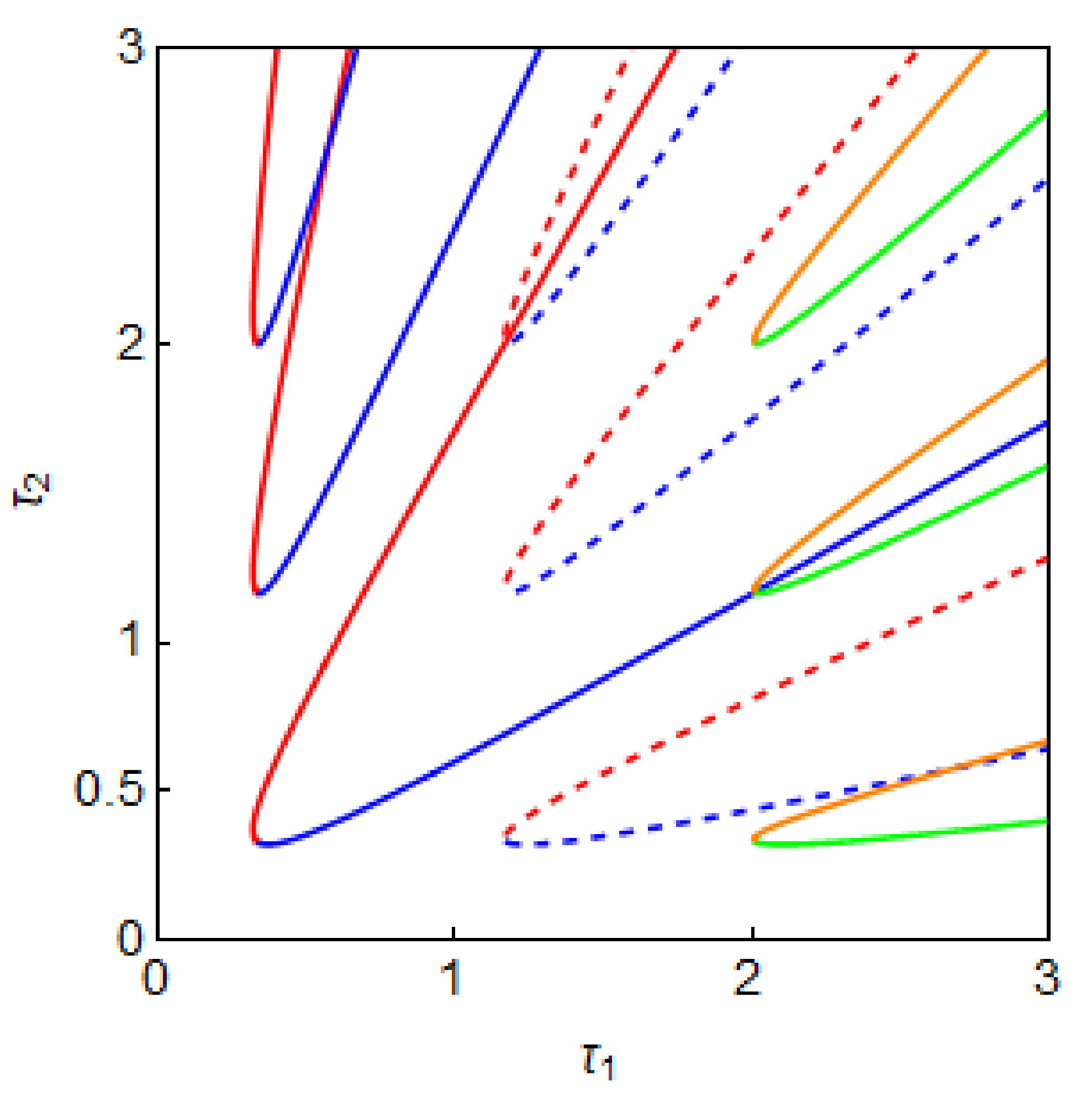
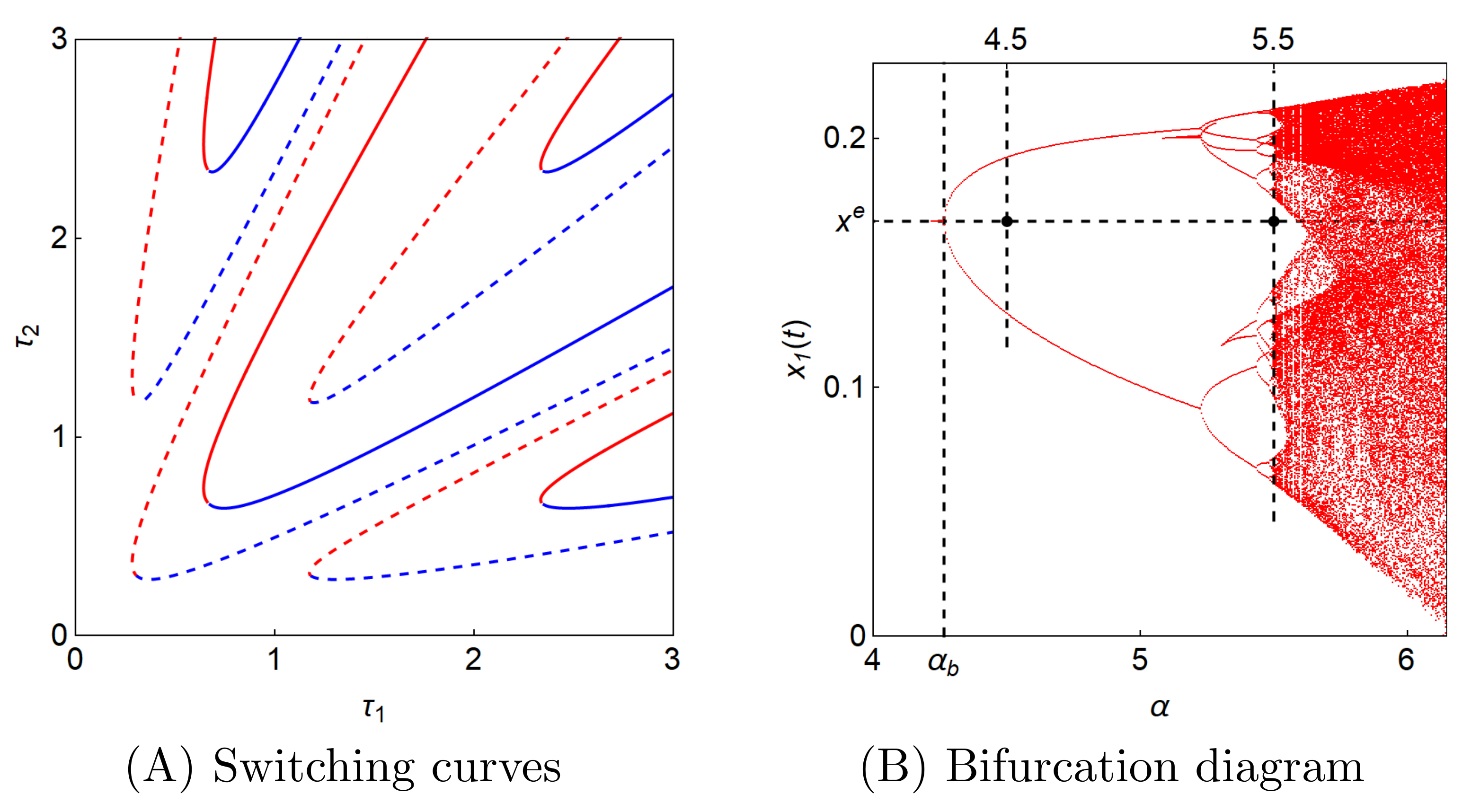
In the first example, we examine the roles of $\sigma$ representing the inertia in the production process. Taking fixed values of $(m,n)=0,1$ and $\alpha =5.5$, we illustrate the solid switching curves with $\sigma =0.1$ and the dotted switching curve with $\sigma =0.2$ in Figure 4A. The curve with $m=n=0$ has the connecting point of the two branches in the lower part of the diagonal. The connecting point of the solid curve is

$${\tau }_{1,0}^{+}\left({\omega }_1\right)={\tau }_{1,0}^{-}\left({\omega }_1\right)\simeq 0.3035$$

$${\tau }_{2,0}^{-}\left({\omega }_1\right)={\tau }_{1,0}^{+}\left({\omega }_1\right)\simeq 0.3035$$

where ${\omega }_1=\tilde{\omega }$, and increasing m shifts it rightward, increasing n shifts it upward while the curve with $m=n=1$ is located upper-right. It is observed that the dotted curves move further away from the origin than the solid curves, implying that increasing $\sigma$ enlarges the stability region. The dotted point $({\tau }_1,{\tau }_2)=(1,1)$ is located within the corn-shaped instability regions for $\sigma =0.1$ and $\sigma =0.2$. However, as the value of $\sigma$ increases, the switching curves shift in the upper-right direction, and in consequence, the dotted point becomes located in the stable region for $\sigma >{\sigma }_s\simeq 0.659$. 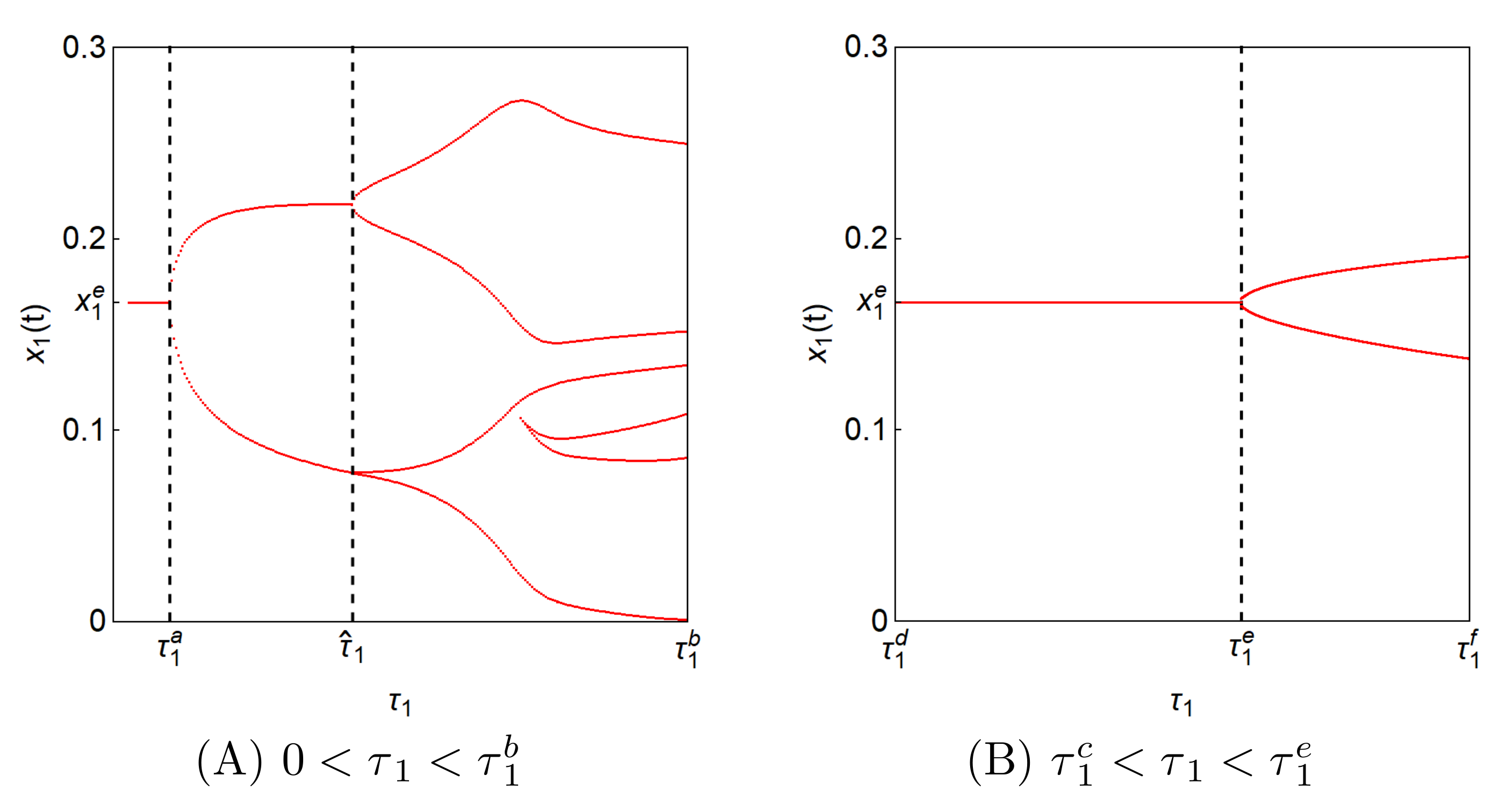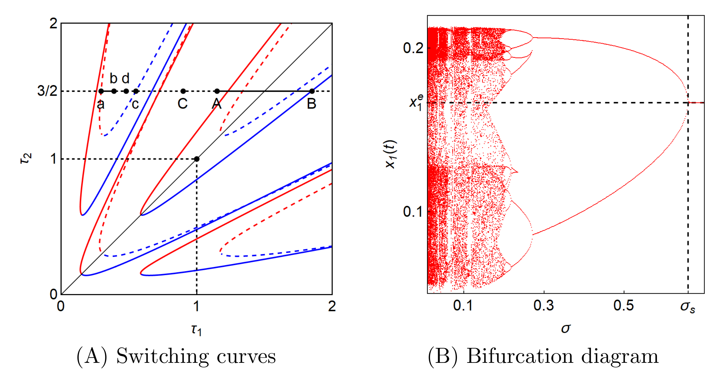This $\sigma$-stabilizing effect can be demonstrated more prominently in the bifurcation diagram for $\sigma$ in Figure 4B. We choose $\sigma$ as a bifurcation parameter there and increase its value from $0.01$ to $0.7$ in steps of $0.0002$. For each value of $\sigma$, dynamic system (2) is run for $0\le t\le 1000$ under the parametric specification of

$$x_1^0=0.001,x_2^0=0.002,{\tau }_1={\tau }_2=1,m=n=0.$$

Discarding the data for $t\le 950,$ we plot the local maxima and minima obtained from the remaining data vertically above the selected value of $\sigma$. Increasing the value of $\sigma ,$ we repeat the same procedure until $\sigma$ arrives at $0.7$. The diagram shows that complex dynamics can arisefor smaller values of $\sigma ,$ due to the fact that the dynamic structure with the Berezowski transformation is similar to that of the discrete-time system that exhibits complex dynamics. As $\sigma$ increases, the complicated dynamics gradually disappear through a period-halving cascade. The fixed point is finally stabilized when the value of $\sigma$ arrives at ${\sigma }_s$ and increases. These results are summarized as follows:

Proposition 3.

The inertia σ of dynamic system (2) has a twofold stabilizing effect in the sense that with increasing values, it $\left(i\right)$ enlarges the stability region and $\left(ii\right)$ simplifies the complicated dynamics through a period-halving cascade.

In the second example, we cfocus on the roles of $\alpha$ representing the relative speed of production adjustment. To explore this $\alpha$-effect, we take $\sigma =0.2$ and plot the solid stability switching curves with $\alpha =4.5$ and the dotted switching curves with $a=5.5$ in Figure 5A. The relative locations of the curves depend on the values of m and n as in Figure 4A. It shows that the dotted curves are closer to the origin than the solid curves. Hence, increasing the value of $\alpha$ shrinks the stability region. The bifurcation diagram for $\alpha$ is illustrated with $\sigma =0.2$. It confirms the $\alpha$-destabilizing effect in which the fixed point with ${\tau }_1={\tau }_2=1$ loses stability for $\alpha ={\alpha }_b\simeq 4.264$. It is also seen that a limit cycle appears for $\alpha =4.5$, a cycle with many periods for $\alpha =5.5$ and erratic oscillations for larger values of $\alpha$. These results are summarized as follows:

Proposition 4.

The adjustment speed α has a twofold destabilizing effect in the sense that with increasing values, it $\left(i\right)$ contracts the stability region and $\left(ii\right)$ complicates simple dynamics through a period-doubling cascade.

Next, we take a closer look at the global dynamic behavior for ${\tau }_1$ and ${\tau }_2$. Therefore, we carry out more numerical simulations with the following parameters. For any other parameter specification, we might obtain the same qualitative results.

$$\alpha =5.5,\sigma =0.1\mathrm{and}{\tau }_2=1.5$$

and the initial conditions,

$$x_1^0=0.01\mathrm{and}{x}_2^0=0.02.$$

We increase the value of ${\tau }_1$ along the horizontal segment $ab$ in the upper-left corner in Figure 4A. In this study, the firms are identical under Assumptions 1 and 3, and the resultant stability switching curves are symmetric for the diagonal. In consequence, varying ${\tau }_1$ and fixing ${\tau }_2$ and fixing ${\tau }_1$ and varying ${\tau }_2$ can generate the same results. Notice that the horizontal line at ${\tau }_2=1.5$ crosses the upper-left corn-shaped dotted curve twice at

$${\tau }_1^a\simeq 0.295\mathrm{and}{\tau }_1^c\simeq 0.552.$$

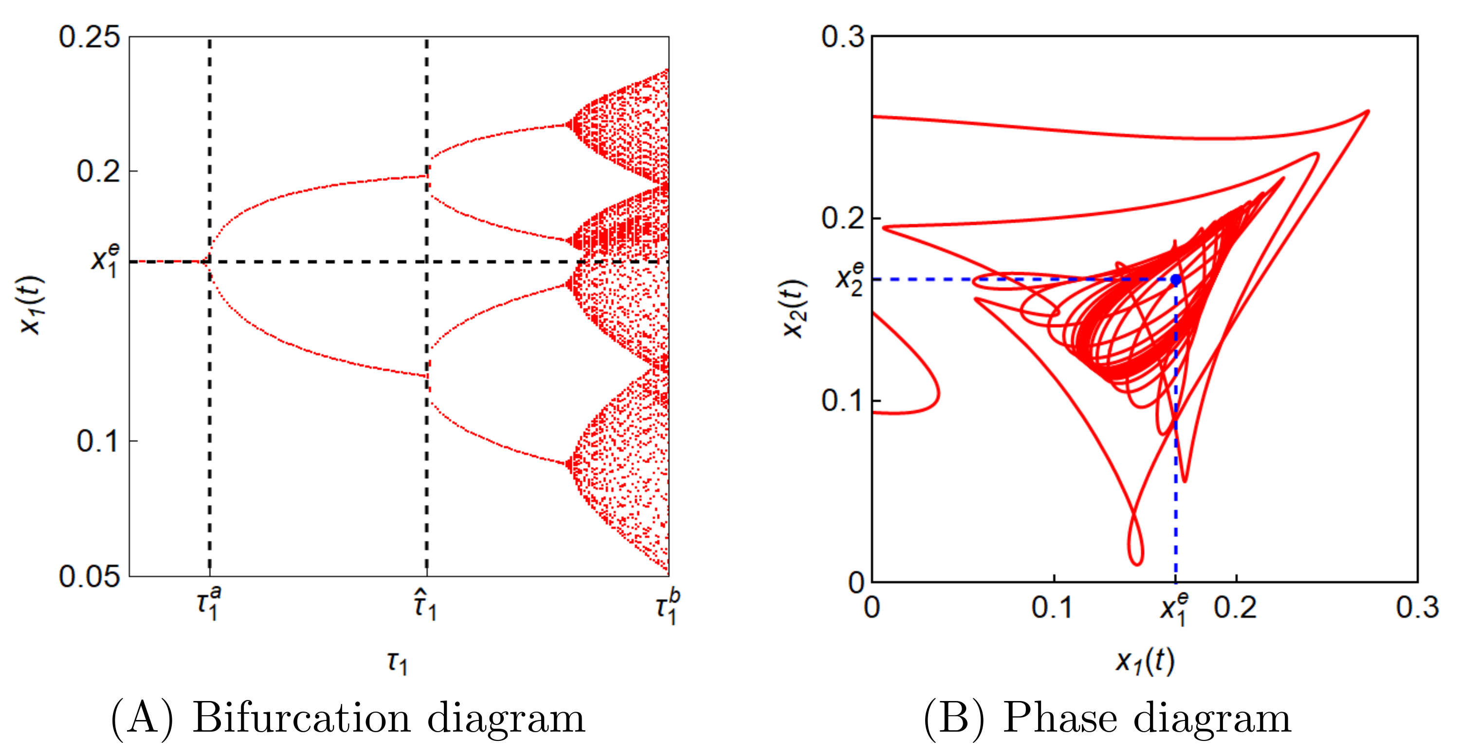
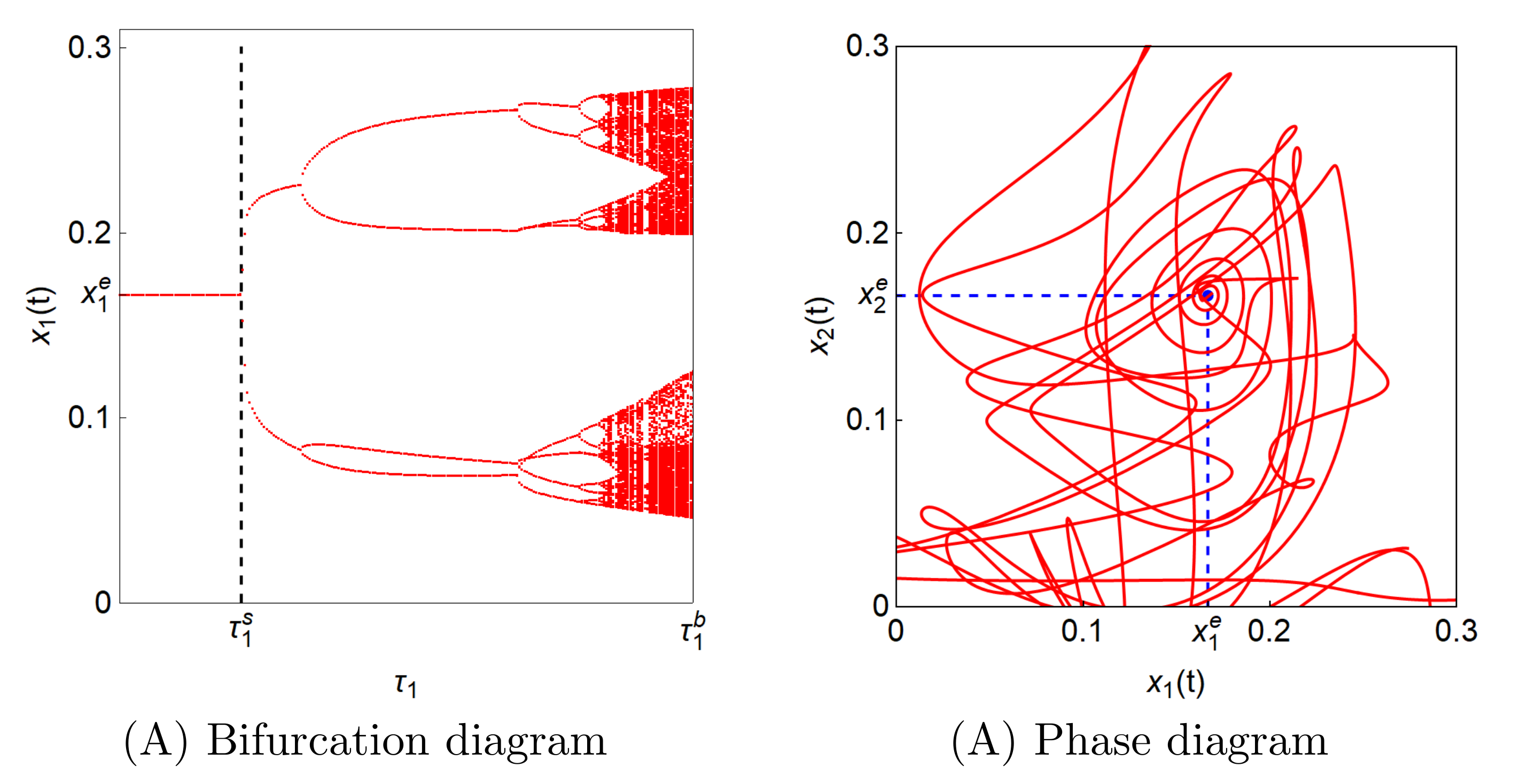
The first result is described by the bifurcation diagram in Figure 6(A) in which ${\tau }_1\in [{\tau }_1^a-p,{\tau }_1^b]$, $p>0$ is a small number and ${\tau }_1^b=0.38$. For ${\tau }_1<{\tau }_1^a,$ there is a stable fixed point. We can see that an interesting phenomenon begins to happen when the value of ${\tau }_1$ exceeds the critical value of ${\tau }_1^a$. For ${\tau }_1={\tau }_1^a,$ the fixed point loses stability and is replaced with a limit cycle. As the value of ${\tau }_1$ increases, the cyclic solution branches to form a doubly cyclic solution at the second bifurcation point near ${\widehat{\tau }}_1\simeq 0.335$. This value is a rough estimation. Further increasing ${\tau }_1$ to ${\tau }_1^b$ gives rise to a third bifurcation, after which much more complicated oscillations emerge. For ${\tau }_1>{\tau }_1^b,$ the dynamic system generates trajectories that might be negative, as is demonstrated in Figure 6B. The model is not well-behaved and loses its economic meaning. However, for ${\tau }_1$ just a little bit smaller than ${\tau }_1^c,$ a limit cycle is obtained again and then the fixed point regains stability for ${\tau }_1={\tau }_1^c.$Figure 6B shows the second result obtained for ${\tau }_1^d=0.48$ that is between ${\tau }_1^b$ and ${\tau }_1^c.$ It displays an expanding phase diagram in which $x_1\left(t\right)$ oscillates around the fixed point denoted by the blue dot for a while but gradually moves away from it, finally becomes negative for some values of t.

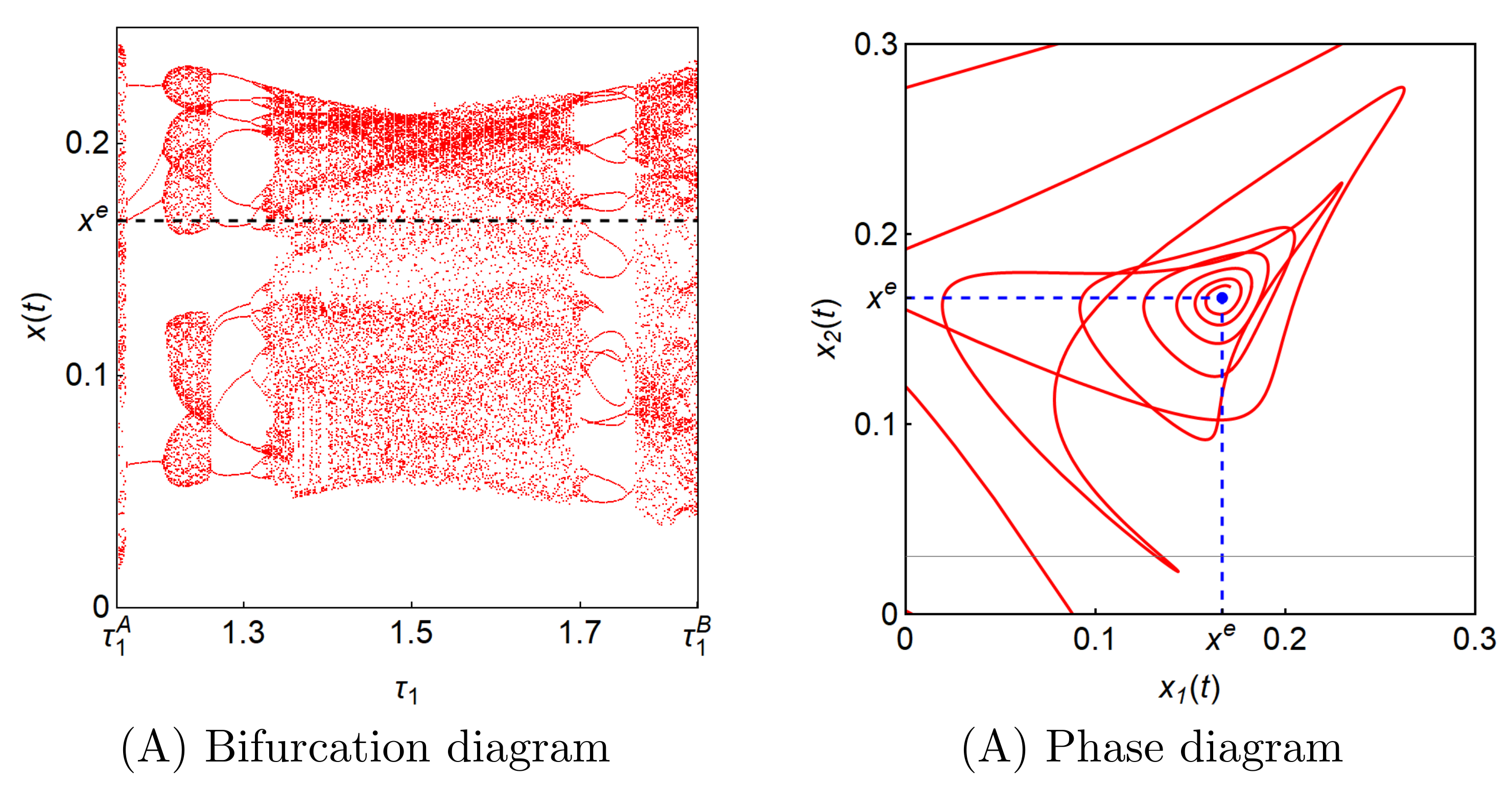
Under the same parameter set, we carry out the fourth example. Its result is illustrated in Figure 4A when the value of ${\tau }_1$ increases along the segment $AB.$ The extreme values of ${\tau }_1$ are

$${\tau }_1^A\simeq 1.15\mathrm{and}{\tau }_1^B\simeq 1.85.$$

Notice that the segment $AB$ is located within the largest dotted corn-shaped stability switching curve. The fixed point is unstable for ${\tau }_1\in [{\tau }_1^A,{\tau }_1^B]$. As compared to Figure 6A, we present Figure 7A in which the bifurcation diagram for ${\tau }_1$ within this interval undergoes more complicated motions. The solution of the system bifurcates to erratic oscillations from regular oscillations and vice versa. A bit after ${\tau }_1={\tau }_1^A,$ a regular cycle is clearly seen, which proceeds to spreading oscillations and then a regular cycle again with more periodicity appears as ${\tau }_1$ increases. However, just raising ${\tau }_1$ slightly from ${\tau }_1^B$ or lowering it from ${\tau }_1^A$, we find unfavorable trajectories that sooner or later take negative values. Figure 7B illustrates a phase portrait for ${\tau }_1^C=0.9<{\tau }_1^A$. The time trajectory oscillates around the fixed point for smaller values of t but gets out of the nonnegative region for larger values. The numerical results obtained along the horizontal line at ${\tau }_2=1.5$ are summarized as follows:

Proposition 5.

For the fixed value of ${\tau }_2=3/2,$ a solution of delay system $\left(\right)$ exhibits various dynamics ranging from a limit cycle to an erratic oscillation as ${\tau }_1$ increases. Further, some solution could be negative and thus loses its economic meaning.

4.2. The Case Including $A=0$

We now draw attention to the dynamic behavior under

$$\alpha =10,\sigma =0.1,m=n=0$$

for which $4<\alpha (1-c)<6$ holds. From $x_i$ for $i=1,2,3,4$ in (12),

$$x_4<0<x_2=x_3<x_1.$$

Let $\tilde{\omega }=\sqrt{x_1}$ and $\overline{\omega }$ defined in (8) is equal to $\sqrt{x_2}=\sqrt{x_3}$ where

$$\overline{\omega }=\sqrt{\frac{\alpha (1-c)\left[\alpha (1-c)-4\right]}{3{\sigma }^2}}=10\sqrt{5/3}\simeq 12.91$$

and

$$\tilde{\omega }=\sqrt{\frac{\alpha (1-c)\left[\alpha (1-c)-2\right]}{{\sigma }^2}}=10\sqrt{15}\simeq 38.73.$$

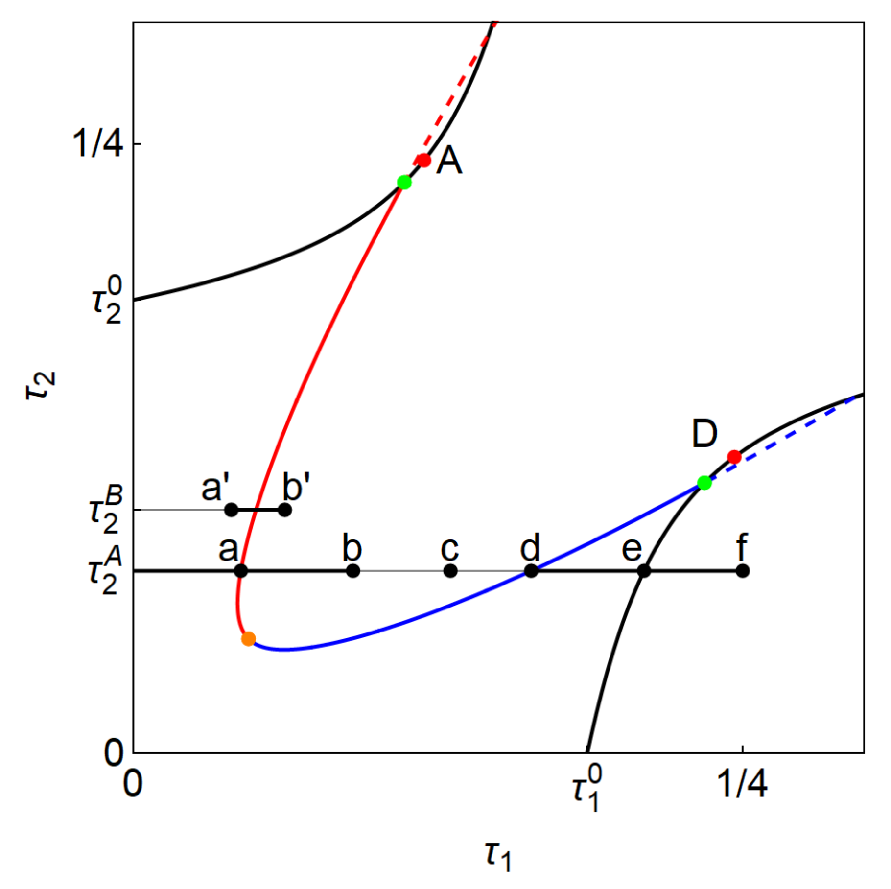
The black curves in Figure 8 are the same as those in Figure 3 in which $\omega =\overline{\omega }$. Applying Theorem 3 with the newly specified values of the parameters, we obtain that the solid red-blue curve is loci of

$$({\tau }_{1,m}^{+}\left(\omega \right),{\tau }_{2,n}^{-}\left(\omega \right))\mathrm{and}({\tau }_{1,m}^{-}\left(\omega \right),{\tau }_{2,n}^{+}\left(\omega \right))\mathrm{for}\omega \in (\overline{\omega },\tilde{\omega })\mathrm{and}m=n=0$$

whereasthe dotted red-blue curves as loci of

$$({\tau }_{1,m}^{+}\left(\omega \right),{\tau }_{2,n}^{-}\left(\omega \right))\mathrm{with}\left(m,n\right)=\left(1,0\right)$$

and

$$({\tau }_{1,m}^{-}\left(\omega \right),{\tau }_{2,n}^{+}\left(\omega \right))\mathrm{with}\left(m,n\right)=\left(0,1\right)\mathrm{for}\omega \in (0,\overline{\omega })$$

where ${\varphi }_1\left(\omega \right)$ and ${\varphi }_2\left(\omega \right)$ in (13) and (16) are re-defined as

$${\varphi }_1\left(\omega \right)={tan}^{-1}\left(\frac{B_1\left(\omega \right)}{A_1\left(\omega \right)}\right)\mathrm{and}{\varphi }_2\left(\omega \right)={tan}^{-1}\left(\frac{B_2\left(\omega \right)}{A_2\left(\omega \right)}\right).$$

Notice that $A=0$ along the black curves, $A<0$ along the dotted curves and $A>0$ along the solid curves.

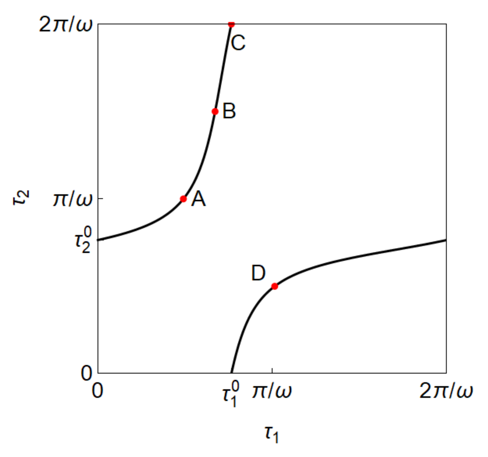
The stability region including the origin is surrounded by the upper black curve starting at ${\tau }_2^0$ on the vertical axis, the solid red-blue segment and the lower black curve ending at ${\tau }_1^0$ on the horizontal axis. Points A and D are those shown in Figure 3. The orange point is the connecting point of the blue and red segments,

$$({\tau }_{1,0}^{+}\left(\tilde{\omega }\right),{\tau }_{2,0}^{-}\left(\tilde{\omega }\right))=({\tau }_{1,0}^{-}\left(\tilde{\omega }\right),{\tau }_{2,0}^{+}\left(\tilde{\omega }\right))\simeq (0.047,0.047)$$

and the green points are on the black curves,

$$({\tau }_{1,0}^{+}\left(\overline{\omega }\right),{\tau }_{2,0}^{-}\left(\overline{\omega }\right))=({\tau }_{2,0}^{+}\left(\overline{\omega }\right),{\tau }_{1,0}^{-}\left(\overline{\omega }\right))\simeq (0.234,0.111).$$

These green points are asymmetric with respect to the diagonal, the starting points of the solid curves and the end points of the dotted curves.

We present some numerical results to observe what dynamics system (2) can generate. The red and blue segments correspond to the case of $A\ne 0$ and the case of $A=0$ is shown by the two black segments. Let ${\tau }_2^A=0.075$ and choose ${\tau }_1$ as a bifurcation parameter. The horizontal line at ${\tau }_2={\tau }_2^A$ crosses the stability switching curve three times whose ${\tau }_1$-coordinates are

$${\tau }_1^a\simeq 0.044,{\tau }_1^d\simeq 0.163\mathrm{and}{\tau }_1^e\simeq 0.209.$$

The fixed point is asymptotically stable for ${\tau }_1<{\tau }_1^a,$ loses its stability at ${\tau }_1={\tau }_1^a$ and undergoes a Hopf bifurcation. It regains stability at ${\tau }_1={\tau }_1^d$ and then loses stability again at ${\tau }_1={\tau }_1^e$. Although it is known that the fixed point is unstable for ${\tau }_1\in [{\tau }_1^a,{\tau }_1^d)$ and ${\tau }_1>{\tau }_1^e,$ it is not known what kind of dynamics could emerge. For this reason, we perform simulations, focusing on the unstable intervals. Figure 9A describes possible dynamics for ${\tau }_1\in \left[{\tau }_1^a-p,{\tau }_1^b\right]$ with ${\tau }_1^b=0.09$ and p is a small number. The Hopf value is ${\tau }_1^a.$ A cyclic solution occurs for ${\tau }_1>{\tau }_1^a$ and its amplitude gets larger as ${\tau }_1$ becomes larger. The second bifurcation takes place around ${\widehat{\tau }}_1\simeq 0.06$ (This value is also a rough estimation.)and periodicity of the cycle is doubled. Figure 9B is a bifurcation diagram for ${\tau }_1\in \left[{\tau }_1^d,{\tau }_1^f\right]$ with ${\tau }_1^f=0.25.$ A Hopf bifurcation occurs at ${\tau }_1={\tau }_1^e$ and the stable fixed point for ${\tau }_1<{\tau }_1^e$ bifurcates to a limit cycle for ${\tau }_1>{\tau }_1^e.$

Two more examples are given to explore the occurrence of stability switching. We change only the value of ${\tau }_2$ from $0.075$ to $0.1(={\tau }_2^B),$ keeping other parameter values fixed as given. Figure 10A shows that delay system (2) undergoes a period-doubling bifurcation for ${\tau }_1\in [{\tau }_1^{a^{\prime }},{\tau }_1^{b^{\prime }}]$ with ${\tau }_1^{a^{\prime }}=0.04$ and ${\tau }_1^{b^{\prime }}=0.062$ along the horizontal curve at ${\tau }_2^B.$ The solution can exchange its form (stable point, limit cycle, period-doubling and chaos) for different values of ${\tau }_1.$ Comparing Figure 10A with Figure 9A indicates that system (2) apparently generates more complicated dynamics involving the transition from order to chaos when ${\tau }_2$ is increased. The next example in Figure 10B is a phase diagram at point c with ${\tau }_1=0.13$ between points b and c in Figure 8. It indicates that system (2) possesses exploded dynamics for bifurcation parameter ${\tau }_1$ in the range of $[{\tau }_1^b,{\tau }_1^c].$ A trajectory starting in the neighborhood of the fixed point oscillatory moves away, repeat erratic ups and downs several times and then crosses the horizontal or vertical axis. Crossing the axis means that such a trajectory takes a negative value and loses its economic meaning. Similar exploded results are obtained for the different values of ${\tau }_1$ and ${\tau }_2$.

5. Concluding Remarks

This paper is based on the model given by [11], which used a special transformation of discrete time duopoly models into continuous models and investigated the asymptotical behavior of the equilibrium when two discrete delays were present. Several cases were examined. This paper reexamines this model and in a two-dimensional analysis, the stability switching curves were analytically determined and illustrated. The analysis was performed in two parts depending on model parameters. Two different sets of stability switching curves were determined. In the first case, for each value of $\omega$, the set of corresponing values of the delays were determined giving a collection of curves. The second case appears with a special value $\omega$, when one delay can have an arbitrary value and the other delays are its function. With increasing values of m and n, continuous curves were determined. Numerical simulations verified the theoretical results, and a detailed sensitivity analysis was performed. It was illustrated that both the inertia coefficient and the speed of adjustments have twofold effects on the stability of the equilibrium: the inertia coefficient enlarges the stability region and simplifies the complicated dynamics with period-halving cascade, while the adjustment speed contracts the stability region and complicates dynamics through a period-doubling bifurcation. In the analysis, the most simple linear duopoly model was considered. More complex linear and even nonlinear duopoly models could be the subject of future studies. To preserve the dimension of the model, a semi-symmetric n-firm oligopoly could be examined, which has two groups, with each group having identical firms.