Article

Convergence and Stability of a Parametric Class of Iterative Schemes for Solving Nonlinear Systems

by
Alicia Cordero
,
Eva G. Villalba
,
Juan R. Torregrosa
* and
Paula Triguero-Navarro
Multidisciplinary Institute of Mathematics, Universitat Politènica de València, 46022 València, Spain
*
Author to whom correspondence should be addressed.
Submission received: 1 December 2020 / Revised: 22 December 2020 / Accepted: 24 December 2020 / Published: 3 January 2021
(This article belongs to the Special Issue Mathematical Methods, Modelling and Applications)

Abstract

:
A new parametric class of iterative schemes for solving nonlinear systems is designed. The third- or fourth-order convergence, depending on the values of the parameter being proven. The analysis of the dynamical behavior of this class in the context of scalar nonlinear equations is presented. This study gives us important information about the stability and reliability of the members of the family. The numerical results obtained by applying different elements of the family for solving the Hammerstein integral equation and the Fisher’s equation confirm the theoretical results.

1. Design of a Parametric Family of Iterative Methods

The need to find a solution x ¯ of equations or systems of nonlinear equations of the form F ( x ) = 0 , where F : D R n R n , n 1 , is present in many problems of applied mathematics as a basis for solving other more complex ones. In general, it is not possible to find the exact solution to this type of equations, so iterative methods are required in order to approximate the desired solution.
The essence of these methods is to find, through an iterative process and, from an initial approximation x ( 0 ) close to a solution x ¯ , a sequence { x ( k ) } of approximations such that, under different requirements, lim k x ( k ) = x ¯ .
It is well known that one of the most used iterative methods, due to its simplicity and efficiency, is Newton’s scheme, whose iterative expression is
x ( k + 1 ) = x ( k ) [ F ( x ( k ) ) ] 1 F ( x ( k ) ) , k = 0 , 1 , 2 ,
where F ( x ( k ) ) denotes the derivative or the Jacobian matrix of function F evaluated in the kth iteration x ( k ) . In addition, this method has great importance in the study of iterative methods because it presents quadratic convergence under certain conditions and has great accessibility, that is, the region of initial estimates x ( 0 ) for which the method converges is wide, at least for polynomials or polynomial systems.
Based on Newton-type methods and by using different procedures, many iterative schemes for solving F ( x ) = 0 have been presented in the last years. Refs. [1,2] compile many of the methods recently designed to solve this type of problem. These books give us good overviews about this area of research.
In this paper, we use a convex combination of the methods presented by Chun et al. in [3] and Maheswari in [4]. As the mentioned schemes are designed for nonlinear equations and they have as the first step Newton’s method, we use the following algebraic manipulation in order to extend the mentioned schemes to nonlinear systems:
f ( y ( k ) ) f ( x ( k ) ) = f ( y ( k ) ) ( x ( k ) y ( k ) ) f ( x ( k ) ) = f ( y ( k ) ) f ( x ( k ) ) + f ( x ( k ) ) ( x ( k ) y ( k ) ) f ( x ( k ) ) = [ x ( k ) , y ( k ) ; f ] f ( x ( k ) ) + 1 .
Therefore, the parametric family of iterative methods for solving nonlinear systems that we propose has the following iterative expression:
y ( k ) = x ( k ) F ( x ( k ) ) 1 F ( x ( k ) ) , H ( x ( k ) , y ( k ) , γ ) = I + γ 2 I + ( 1 γ ) B k 1 ( 1 γ ) B k ( 2 I B k ) γ 2 F ( x ( k ) ) 1 F ( y ( k ) ) x ( k + 1 ) = x ( k ) H ( x ( k ) , y ( k ) , γ ) F ( x ( k ) ) 1 F ( x ( k ) ) for k = 0 , 1 , 2 , ,
where x ( 0 ) is the initial estimation, B k = F ( x ( k ) ) 1 P ( k ) and P ( k ) = [ x ( k ) , y ( k ) ; F ] is the divided difference operator defined as
[ x , y ; F ] ( x y ) = F ( x ) F ( y ) , x , y R n .
The rest of the paper is organized as follows: Section 2 is devoted to analyze the convergence of family (2) in terms of the values of parameter γ . In Section 3, we study the dynamical behavior of the class on quadratic polynomials in the context of scalar equations. This study allows for selecting the members that are more stable in the family. In the numerical section, (Section 4), we apply the proposed class on different examples such as the Hammerstein integral equation and the Fisher’s equation in order to confirm the theoretical results obtained in Section 2 and Section 3. We finish the work with some conclusions and the references used in it.

2. Convergence Analysis

Let us consider function F : D R n R n , differentiable in the convex set D R n which contains a solution x ¯ of the nonlinear equation F ( x ) = 0 . From the Genochi–Hermite formula (see [5]) of the divided difference operator
[ x + h , x ; F ] = 0 1 F ( x + t h ) d t
and by performing the Taylor’s expansion of F ( x + t h ) on the point x and integrating, we obtain the following development:
[ x + h , x ; F ] = F ( x ) + 1 2 F ( x ) h + 1 6 F ( x ) h 2 + O ( h 3 ) ,
which we will use in the proof of the following result, when the order of convergence of family is established.
Theorem 1.
Let F : D R n R n be a sufficiently Fréchet differentiable function in a convex neighborhood D of x ¯ , being F ( x ¯ ) = 0 . We suppose the Jacobian matrix F ( x ) is continuous and non-singular in x ¯ . Then, taking an initial estimate x ( 0 ) close enough to x ¯ , the sequence of iterates { x ( k ) } generated with family (2) converges to x ¯ with the following error equation:
e k + 1 = γ 2 ( C 3 + 4 C 2 2 ) e k 3 + ( γ C 4 + ( 4 13 γ ) C 2 3 + 3 γ C 2 C 3 + ( 1 + 5 2 γ ) C 3 C 2 ) e k 4 + O ( e k 5 ) ,
where C j = 1 j ! F ( α ) 1 F ( j ) ( α ) L j ( R n , R n ) , L j ( R n , R n ) being the set of j-linear functions of bounded functions, j = 2 , 3 , and e k = x ( k ) x ¯ . In the particular case in which γ = 0 , the error equation is
e k + 1 = ( 4 C 2 3 C 3 C 2 ) e k 4 + O ( e k 5 ) ,
and so the method has an order of convergence four.
Proof. 
We consider the Taylor’s expansion of F ( x ( k ) ) around x ¯ :
F ( x ( k ) ) = Γ e k + C 2 e k 2 + C 3 e k 3 + C 4 e k 4 + C 5 e k 5 + O ( e k 6 ) ,
where Γ = F ( x ¯ ) , e k = x ( k ) x ¯ and C j = F ( x ¯ ) 1 F ( j ) ( x ¯ ) j ! L j ( R n , R n ) , j = 2 , 3 ,
In a similar way, the derivatives of F ( x ( k ) ) around x ¯ take the form:
F ( x ( k ) ) = Γ I + 2 C 2 e k + 3 C 3 e k 2 + 4 C 4 e k 3 + 5 C 5 e k 4 + O ( e k 5 ) , F ( x ( k ) ) = Γ 2 C 2 + 6 C 3 e k + 12 C 4 e k 2 + 20 C 5 e k 3 + O ( e k 4 ) , F ( x ( k ) ) = Γ 6 C 3 + 24 C 4 e k + 60 C 5 e k 2 + O ( e k 3 ) .
From the development of F ( x ( k ) ) around x ¯ , we calculate the inverse
F ( x ( k ) ) 1 = I + X 2 e k + X 3 e k 2 + X 4 e k 3 + X 5 e k 4 Γ 1 + O ( e k 5 ) ,
with X 2 , X 3 , X 4 and X 5 satisfying F ( x ( k ) ) 1 F ( x ( k ) ) = I .
Therefore,
  • X 2 = 2 C 2 ,
  • X 3 = 4 C 2 2 3 C 3 ,
  • X 4 = 8 C 2 3 + 6 C 2 C 3 + 6 C 3 C 2 4 C 4 ,
  • X 5 = 16 C 2 4 + 9 C 3 2 + 8 C 2 C 4 + 8 C 4 C 2 12 C 2 2 C 3 12 C 2 C 3 C 2 12 C 3 C 2 2 5 C 5 .
Applying (7) and (9), we obtain
F ( x ( k ) ) 1 F ( x ( k ) ) = e k C 2 e k 2 + ( 2 C 3 + 2 C 2 2 ) e k 3 + ( 3 C 4 + 4 C 2 C 3 + 3 C 3 C 2 4 C 2 3 ) e k 4 + O ( e k 5 ) .
Then, we obtain the error equation of the first step of the parametric family (2):
y ( k ) x ¯ = x ( k ) x ¯ F ( x ( k ) ) 1 F ( x ( k ) ) = = C 2 e k 2 + ( 2 C 3 2 C 2 2 ) e k 3 + ( 3 C 4 4 C 2 C 3 3 C 3 C 2 + 4 C 2 3 ) e k 4 + O ( e k 5 ) .
Substituting this expression in the Taylor expansion of F ( y ( k ) ) around x ¯ , we get:
F ( y ( k ) ) = Γ C 2 e k 2 + ( 2 C 3 2 C 2 2 ) e k 3 + ( 3 C 4 4 C 2 C 3 3 C 3 C 2 + 5 C 2 3 ) e k 4 + O ( e k 5 ) .
Furthermore,
F ( y ( k ) ) = Γ I + 2 C 2 2 e k 2 + ( 4 C 2 C 3 4 C 2 3 ) e k 3 + ( 6 C 2 C 4 8 C 2 2 C 3 6 C 2 C 3 C 2 + 8 C 2 4 + 3 C 3 C 2 2 ) e k 4 + O ( e k 5 ) .
Multiplying expressions (9) and (13), we obtain:
F ( x ( k ) ) 1 F ( y ( k ) ) = I 2 C 2 e k + ( 3 C 3 + 6 C 2 2 ) e k 2 + ( 4 C 4 + 10 C 2 C 3 + 6 C 3 C 2 16 C 2 3 ) e k 3 + + ( 5 C 5 + 14 C 2 C 4 + 9 C 3 2 28 C 2 2 C 3 + 8 C 4 C 2 18 C 2 C 3 C 2 15 C 3 C 2 2 + 40 C 2 4 ) e k 4 + + O ( e k 5 ) .
To obtain the development of the divided difference operator of (2), we use the Taylor series expansion of (4), considering in this case x + h = y and, so, h = y x = F ( x ( k ) ) 1 F ( x ( k ) ) . Therefore, substituting (8) and (10) in (4), we obtain
[ x ( k ) , y ( k ) ; F ] = Γ [ I + C 2 e k + ( C 3 + C 2 2 ) e k 2 + ( C 4 + C 3 C 2 + 2 C 2 C 3 2 C 2 3 ) e k 3 + + ( C 5 + C 4 C 2 + 2 C 3 2 C 3 C 2 2 + 3 C 2 C 4 4 C 2 2 C 3 3 C 2 C 3 C 2 + 4 C 2 4 ) e k 4 ] + O ( e k 5 ) .
To calculate the inverse of this operator, we search
[ x ( k ) , y ( k ) ; F ] 1 = I + Y 2 e k + Y 3 e k 2 + Y 4 e k 3 + Y 5 e k 4 Γ 1 + O ( e k 5 ) ,
with Y 2 , Y 3 , Y 4 and Y 5 satisfying [ x ( k ) , y ( k ) ; F ] 1 [ x ( k ) , y ( k ) ; F ] = I .
Thus,
  • Y 2 = C 2 ,
  • Y 3 = C 3 ,
  • Y 4 = C 4 C 2 C 3 + 3 C 2 3 ,
  • Y 5 = C 5 2 C 2 C 4 9 C 2 4 C 3 2 + 2 C 3 C 2 2 + 6 C 2 2 C 3 + 5 C 2 C 3 C 2 .
Now, using (9) and (15), we obtain B k ,
B k = C 2 2 e k 2 + ( 2 C 2 C 3 + 2 C 3 C 2 6 C 2 3 ) e 3 + + ( 3 C 2 C 4 10 C 2 C 3 C 2 12 C 2 2 C 3 + 25 C 2 4 + 4 C 3 2 10 C 3 C 2 2 + 3 C 4 C 2 ) e k 4 + O ( e k 5 ) ,
and using (8) and (16), we calculate B K 1 ,
B k 1 = I + C 2 e k + ( 2 C 3 2 C 2 2 ) e k 2 + ( 3 C 4 4 C 2 C 3 2 C 3 C 2 + 3 C 2 3 ) e k 3 + + ( 4 C 5 6 C 2 C 4 2 C 4 C 2 4 C 3 2 3 C 2 4 + 2 C 3 C 2 2 + 3 C 2 C 3 C 2 + 6 C 2 2 C 3 ) e k 4 + O ( e k 5 ) .
Substituting the expressions (10), (14), (17), and (18) in the scheme (2), we get the error equation of the parametric family
e k + 1 = x ( k + 1 ) x ¯ = γ 2 ( C 3 + 4 C 2 2 ) e k 3 + ( γ C 4 + ( 4 13 γ ) C 2 3 + 3 γ C 2 C 3 + ( 1 + 5 2 γ ) C 3 C 2 ) e k 4 + O ( e k 5 ) .
Finally, from the error equation, we conclude that the parametric family (2) has order 3 for all γ 0 and order 4 for γ = 0 , being in this last case the error equation
e k + 1 = ( 4 C 2 3 C 3 C 2 ) e k 4 + O ( e k 5 ) .
In the next section, we analyze the dynamical behavior of the parametric family (2) on quadratic scalar polynomials.

3. Complex Dynamics

The dynamical analysis of (2) is performed throughout this section in terms of complex analysis. The order of convergence is not the only important criterion to study when evaluating an iterative scheme. The validity of a method also depends on other aspects such as knowing how it behaves based on the initial estimates that are taken, that is, how wide the set of initial estimations is for which the method is convergent. For this reason, it is necessary to introduce several tools that allow for a more exhaustive study.
The analysis of the dynamics of a method is becoming one of the most investigated parts within the study of iterative methods since it allows for classifying the different iterative schemes, not only from the point of view of their speed of convergence, but also analyzing its behavior based on the initial estimate taken (see, for example, [6,7,8,9,10,11,12,13]). This study allows for visualizing graphically the set of initial approximations that converge to a given root or to points that are not roots of the equation. In addition, it provides important information about the stability and reliability of the iterative method.
In this paper, we focus on studying the complex dynamic of the parametric family (2) on quadratic polynomials of the form p ( z ) = ( z a ) ( z b ) , where a , b C . For this study, we need to present the result called the Scaling Theorem, since it allows us to conjugate the dynamical behavior of one operator with the behavior associated with another, conjugated through an affine application, that is, our operator has the same stability on all quadratic polynomials. This result will be of great use to us since we can apply the Möbius transformation on the operator R p , γ associated with our parametric family acting on p ( z ) , assuming that the conclusions obtained will be of general application for any quadratic polynomial used.
Theorem 2
(Scaling Theorem for family (2)). Let f ( z ) be an analytic function in the Riemann sphere C ^ and let T ( z ) = α z + β be an affine transformation with α 0 . We consider g ( z ) = λ ( f T ) ( z ) , λ 0 . Let R f , γ and R g , γ be the fixed point operators of the family (2) associated with the functions f and g, respectively, that is to say,
R f , γ ( z ) = z + γ 2 3 f ( y ) f ( z ) + ( 1 γ ) 1 f ( y ) f ( z ) 1 f ( y ) f ( z ) 2 f ( z ) f ( z ) ,
R g , γ ( z ) = z + γ 2 3 g ( y ) g ( z ) + ( 1 γ ) 1 g ( y ) g ( z ) 1 g ( y ) g ( z ) 2 g ( z ) g ( z ) ,
where y = z f ( z ) f ( z ) and z C . Then, R f , γ is analytically conjugated to R g , γ through T, that is to say,
( T R g , γ T 1 ) ( z ) = R f , γ ( z ) .
Proof. 
Taking into account that T ( x y ) = T ( x ) T ( y ) + β , T ( x + y ) = T ( x ) + T ( y ) β and g ( z ) = α λ f ( T ( z ) ) , so
( T R g , γ T 1 ) ( z ) = T ( R g , γ ( T 1 ) ( z ) ) = = T T 1 ( z ) + γ 2 3 g ( T 1 ( y ) ) g ( T 1 ( z ) ) + ( 1 γ ) 1 g ( T 1 ( y ) ) g ( T 1 ( z ) ) 1 g ( T 1 ( y ) ) g ( T 1 ( z ) ) 2 g ( T 1 ( z ) ) g ( T 1 ( z ) ) ,
where y = z g ( z ) g ( z ) , T ( T 1 ( z ) ) = z and
T T 1 ( y ) = T T 1 ( z ) g ( T 1 ( z ) ) g ( T 1 ( z ) ) = T T 1 ( z ) f ( z ) α f ( z ) = z T f ( z ) α f ( z ) + β = z f ( z ) f ( z ) = y .
Therefore, substituting these equalities and simplifying, we have
( T R g , γ T 1 ) ( z ) = = T T 1 ( z ) + γ 2 3 f y f ( z ) + ( 1 γ ) 1 f ( y ) f ( z ) 1 f ( y ) f ( z ) 2 f ( z ) α f ( z ) = z + T γ 2 3 f y f ( z ) + ( 1 γ ) 1 f ( y ) f ( z ) 1 f ( y ) f ( z ) 2 f ( z ) α f ( z ) β = z + T γ 2 3 f y f ( z ) + ( 1 γ ) 1 f ( y ) f ( z ) 1 f ( y ) f ( z ) 2 f ( z ) α f ( z ) ,
then ( T R g , γ T 1 ) ( z ) = R f , γ ( z ) , that is to say, R f , γ and R g , γ are analytically conjugated by T ( z ) . □
Now, we can apply the Möbius transformation on the operator associated with the parametric family (2) in order to obtain an operator that does not depend on the constants a and b and, thus, be able to study the dynamical behavior of this family for any quadratic polynomial. The Möbius transformation, in this case, is h ( z ) = z a z b and has the following properties:
( i ) h ( ) = 1 ( ii ) h ( a ) = 0 ( iii ) h ( b ) = .
The fixed-point rational operator of family (2) on p ( z ) has the expression
O γ ( z ) = ( h R p , γ h 1 ) ( z ) = z 3 2 γ z 2 + 3 γ z + 2 γ + z 5 + 5 z 4 + 10 z 3 + 9 z 2 + 4 z 2 γ z 5 + 3 γ z 4 + 2 γ z 3 + 4 z 4 + 9 z 3 + 10 z 2 + 5 z + 1 .
We can also deduce from (23) that the order of the methods for quadratic polynomials is 3 when γ 0 and 4 when γ = 0 .

3.1. Fixed Points

The orbit of a point z C is defined (see, for example, [14,15]) as the set of the successive applications of the rational operator, i.e.,
z , O γ ( z ) , O γ 2 ( z ) , .
The performance of the orbit of z is deduced attending to its asymptotic behavior. A point x T is said to be T-periodic if O γ T ( z ) = z and O γ t ( z ) z , for t < T . For T = 1 , this point is a fixed point.
Therefore, a fixed point is one that is kept invariant by the operator O γ , that is, it is one that satisfies the equation O γ ( z ) = z . All the roots of the quadratic polynomial are, of course, fixed points of the O γ operator. However, it may happen that fixed points appear that do not correspond to any root; we call these points strange fixed points. These points are not desirable from a numerical point of view because when an initial estimate is taken that is in the neighborhood of a strange fixed point, there is a possibility that the numerical method will converge to it, that is, to a point that is not a solution of the equation. Strange fixed points often appear when iterative methods are analyzed and their presence can show the instability of the method.
Fixed points can be classified according to the behavior of the derivative operator on them; thus, a fixed point z * can be:
  • Repulsor, if | O γ ( z * ) | > 1 ;
  • Parabolic, if | O γ ( z * ) | = 1 ;
  • Attracting, if | O γ ( z * ) | < 1 ;
  • Superattracting, if | O γ ( z * ) | = 0 .
Moreover, the basin of attraction A ( z * ) of an attracting fixed point z * is the set of initial guesses whose orbits tend to z * . Therefore, the set of points whose orbit tends to an attracting fixed point defines the Fatou set F ( O γ ) , while its complement is the Julia set J ( O γ ) .
In what follows, we study what are the fixed points of operator O γ and their character depending on the value of parameter γ . The proof of the following result is straightforward, as it only needs to solve the equation O γ ( z ) = z .
Proposition 1.
By analyzing the equation O γ ( z ) = z , one obtains the following statements:
(i) 
z = 0 and z = are superattracting fixed points for each value of γ.
(ii) 
z = 1 is a strange fixed point when γ 29 7 .
(iii) 
the roots of polynomial
k ( t ) = 1 + 6 t + ( 16 2 γ ) t 2 + ( 21 3 γ ) t 3 + ( 16 2 γ ) t 4 + 6 t 5 + t 6 ,
which we denote by E x i ( γ ) , where i = 1 , 2 , , 6 , are also strange fixed points for each value of γ.
We need the expression of the differentiated operator to analyze the stability of the fixed points and to obtain the critical points:
O γ ( z ) = z 2 ( z + 1 ) 4 γ 6 z 6 + 8 z 5 + 7 z 4 + 7 z 2 + 8 z + 6 + z 16 z 4 + 41 z 3 + 60 z 2 + 41 z + 16 2 γ z 5 + ( 3 γ + 4 ) z 4 + ( 2 γ + 9 ) z 3 + 10 z 2 + 5 z + 1 2 ,
It is clear that 0 and are always superattracting fixed points because they come from the roots of the polynomial, and the order of the iterative methods is higher than 2, but the stability of the other fixed points can change depending on the values of parameter γ .
Proposition 2.
The character of the strange fixed point z = 1 is as follows:
(a) 
If γ = 29 7 , then z = 1 is not a strange fixed point.
(b) 
If R e ( γ ) < 125 7 or R e ( γ ) > 67 7 , then z = 1 is an attracting point.
(c) 
If R e ( γ ) 125 7 , 67 7 and I m ( γ ) 2 + R e ( γ ) + 29 7 2 > 9216 49 , then z = 1 is an attracting point.
(d) 
z = 1 cannot be a superattracting point.
(e) 
If R e ( γ ) 125 7 , 67 7 and I m ( γ ) 2 + R e ( γ ) + 29 7 2 = 9216 49 , then z = 1 is a parabolic point.
(f) 
In another case, z = 1 is the repulsor.
Proof. 
We obtain that
| O γ ( 1 ) | = 96 7 γ + 29 .
It is not difficult to check that | O γ ( 1 ) | cannot be 0, so z = 1 cannot be a superattractor, and, when γ = 29 7 , z = 1 is not a fixed point.
Now, we are going to study when z = 1 is an attracting point. It is easy to check that | O γ ( 1 ) | < 1 is equivalent to 96 2 < | 29 + 7 γ | 2 . Rewriting the last expression, we obtain the following inequality:
8375 < 406 R e ( γ ) + 49 R e ( γ ) 2 + 49 I m ( γ ) 2 .
Let us see when this inequality is verified. When 8375 406 R e ( γ ) 49 R e ( γ ) 2 < 0 , that is, R e ( γ ) 67 7 R e ( γ ) + 125 7 > 0 , z = 1 is an attracting point, so we obtain that z = 1 is an attracting point when R e ( γ ) > 67 7 or R e ( γ ) < 125 7 . When we have R e ( γ ) 125 7 , 67 7 , we need I m ( γ ) to satisfy 8375 < 406 R e ( γ ) + 49 R e ( γ ) 2 + 49 I m ( γ ) 2 , for z = 1 being a superattractor.
We are going to study when z = 1 is a parabolic point. z = 1 will be a parabolic point when 8375 406 R e ( γ ) 49 R e ( γ ) 2 = 49 I m ( γ ) 2 , that is, z = 1 is a parabolic point when R e ( γ ) 125 7 , 67 7 and 49 I m ( γ ) 2 = R e ( γ ) 2 406 R e ( γ ) + 8375 . □
Now, we establish the stability of the strange fixed points that are roots of the polynomial (24). To do this, we calculate these roots noting that this polynomial is a sixth degree symmetric polynomial, that is, it is a polynomial that can be reduced to a third degree one, and that satisfies the following properties:
  • t = 0 is not the root;
  • if t = α is the root, t = 1 α is also the root.
Performing the reduction of (24), we obtain:
1 + 6 t + ( 16 2 γ ) t 2 + ( 21 3 γ ) t 3 + ( 16 2 γ ) t 4 + 6 t 5 + t 6 = 0 ( 1 t 3 + t 3 ) + 6 ( 1 t 2 + t 2 ) + ( 16 2 γ ) ( 1 t + t ) + 21 3 γ = 0 z 3 + 6 z 2 + ( 13 2 γ ) z + 9 3 γ = 0 ,
where z = 1 t + t , z 2 2 = 1 t 2 + t 2 and z 3 3 z = 1 t 3 + t 3 . Now, we calculate the roots of this polynomial and obtain:
z 1 ( γ ) = 2 3 3 ( 2 γ 1 ) 9 γ + 3 γ ( ( 75 32 γ ) γ 78 ) + 93 + 9 3 + 9 γ + 3 γ ( ( 75 32 γ ) γ 78 ) + 93 + 9 3 2 3 3 2 / 3 2 , z 2 ( γ ) = 2 3 3 ( 1 2 γ ) 9 γ + 3 γ ( ( 75 32 γ ) γ 78 ) + 93 + 9 3 + ( 1 ) 2 / 3 9 γ + 3 γ ( ( 75 32 γ ) γ 78 ) + 93 + 9 3 2 3 3 2 / 3 2 , z 3 ( γ ) = ( 1 ) 2 / 3 2 3 3 ( 2 γ 1 ) 9 γ + 3 γ ( ( 75 32 γ ) γ 78 ) + 93 + 9 3 1 2 3 9 γ + 3 γ ( ( 75 32 γ ) γ 78 ) + 93 + 9 3 3 2 / 3 2 .
To calculate the roots of polynomial (24) from the z i ( γ ) , i = 1 , 2 , 3 , we undo the variable change since t = z i ( γ ) ± z i ( γ ) 2 4 2 . Therefore, we obtain the roots of the sixth degree polynomial, which are conjugated two by two
E x 1 ( γ ) = z 1 ( γ ) + z 1 ( γ ) 2 4 2 , E x 2 ( γ ) = z 1 ( γ ) z 1 ( γ ) 2 4 2 , E x 3 ( γ ) = z 2 ( γ ) + z 2 ( γ ) 2 4 2 , E x 4 ( γ ) = z 2 ( γ ) z 2 ( γ ) 2 4 2 , E x 5 ( γ ) = z 3 ( γ ) + z 3 ( γ ) 2 4 2 , E x 6 ( γ ) = z 3 ( γ ) z 3 ( γ ) 2 4 2 .
Now, we study when the roots of the polynomial (24) are superattractors. For them, we solve | O γ ( E x i ( γ ) ) | = 0 for all i = 1 , , 6 , and we get the following relevant values of γ :
  • γ 1 = 0.8114608325277108 ,
  • γ 2 = 5.5908453191613585 ,
  • γ 3 = 0.7671008924094337 + 0.7784254153980097 i ,
  • γ 4 = 0.7671008924094337 0.7784254153980097 i .
Next, we are going to study the character of the fixed points by analyzing those values of γ close to the values of the parameter for which some E x i ( γ ) is a supertractor. To do this, we study how | O γ ( E x i ( γ ) ) | behaves near the four previous values, and we obtain regions where some of the roots will be attractors. These regions are represented in Figure 1.

3.2. Critical Points

The relevance of knowing that the free critical points (that is, critical points different from the roots of the polynomial) is based on this known fact: each invariant Fatou component contains, at least, one critical point. Operator O γ ( z ) has as critical points z = 0 , z = 1 , z = , and the roots of the polynomial
q ( t ) = 6 γ + ( 16 + 8 γ ) t + ( 41 + 7 γ ) t 2 + 60 t 3 + ( 41 + 7 γ ) t 4 + ( 16 + 8 γ ) t 5 + 6 γ t 6 ,
which we denote by Z x i ( γ ) , where i = 1 , , 6 .
Let us remark that z = 1 is a preimage of the fixed point z = 1 . We can see that q ( t ) is a symmetric polynomial, so we can obtain the roots of q ( t ) obtaining roots of a polynomial of degree 3. The polynomial reduced of q ( t ) is the following one that we obtain analogously to the polynomial (24):
q ^ ( t ) = 6 γ t 3 + ( 16 + 8 γ ) t 2 + ( 41 11 γ ) t + 28 16 γ .
In order to calculate the roots z of q ( t ) , we need to obtain the roots of q ^ ( t ) and apply the following expression to them z ± z 2 4 2 . Thus, the roots of q ( t ) are conjugated.
Now, we are going to study the asymptotic behavior of the critical points to establish if there are different convergence basins than those generated by the roots. For the free critical point 1 , we have O γ ( 1 ) = 1 , who is a strange fixed point, so the parameter plane associated with this critical point is not significative, since we know the stability of z = 1 .
The other free critical points are roots of a polynomial that depends on γ ; for that, we draw the parameter planes. As we have that the roots are conjugated, we will only draw three planes. We use as an initial estimate a free critical point that depends on γ . We establish a mesh in the complex plane of 500 × 500 points. Each point of the mesh corresponds to a parameter value. In each of them, the rational function is iterated to obtain the orbit of the critical point as a function of γ . If that orbit converges to z = 0 or to z = in less than 40 iterations, that point of the mesh is painted red; otherwise, the point appears in black.
As we can see, there are many values of the parameter γ that would result in a method in which the free critical points converge to one of the two roots. As it is observed in Figure 2, they are located in the red area on the right side of the plane. Moreover, some black areas can be identified as the regions of stability of those fixed points that can be attracting, such as Figure 1b, whose stability region appears in black on the right side of Figure 2c.
Now, we select some stable (in red in parameter planes) and unstable values of γ (in black) in order to show their performance.
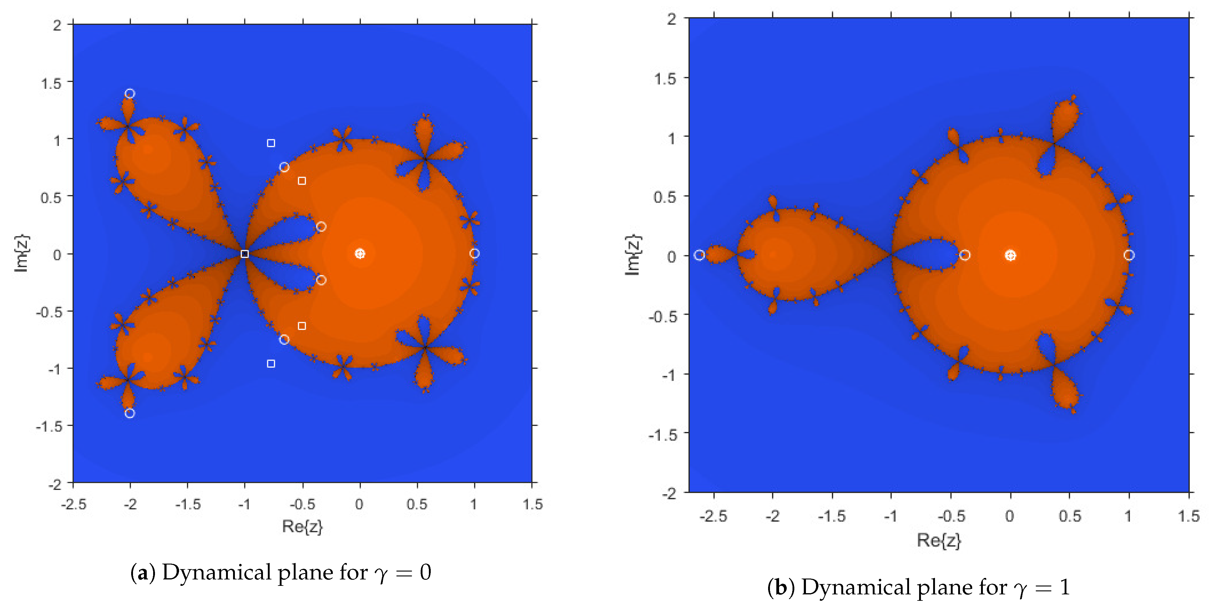
In the case of dynamical planes, the value of the parameter γ is fixed. Each point in the complex plane is considered as a starting point of the iterative scheme, and it is painted in different colors depending on the point that it has converged to. In this case, we paint in blue points what converged to , and in orange points what converged to 0. These dynamical planes have been generated with a mesh of 500 × 500 points and a maximum of 40 iterations per point. We mark strange fixed points with white circles, the fixed point z = 0 with a white star, and free critical points with white squares (again, the routines used appear in [6]).
One value of the parameter that would be an interesting value is γ = 0 because it is the only one that obtains order 4. In that case, we obtain the dynamical plane that we can see in Figure 3a. In this case, two free critical points are in each basin of attraction, and the strange fixed points are in the boundary of both basins of attraction, so they are repulsive. In that case, the method is stable, and, as we can see, almost every point converges to 0 or (Let us notice that, in practice, any initial estimation taken in the Julia set will converge to 0 or to , due to the rounding error).
Other value for the parameter that we study is γ = 1 , Figure 3b. As we can see, this dynamical plane is similar to that of γ = 0 , but, in this case, we obtain less free critical points and less strange fixed points, due to the simplification of the rational function for this value of γ .
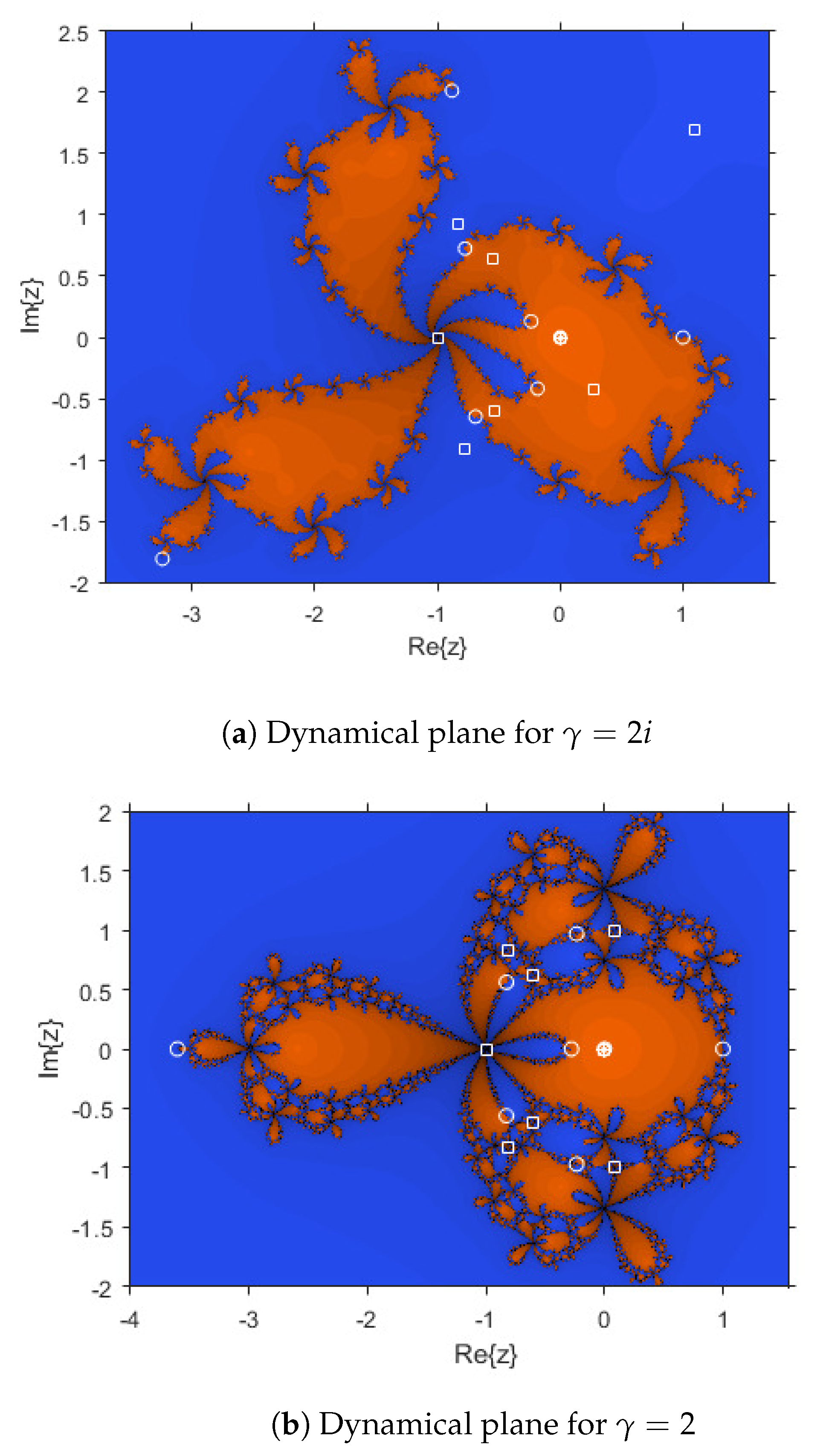
Carrying out numerous experiments, we have realized that the simplest dynamics is that of the methods with parameter γ = 0 and γ = 1 . Next, we will see other dynamical planes associated with other values of the parameter γ . Some of these planes do not have a bad dynamics, although it is not as simple as the previous ones. This is the case of γ = 2 , Figure 4b, or the case of γ = 2 i , Figure 4a.
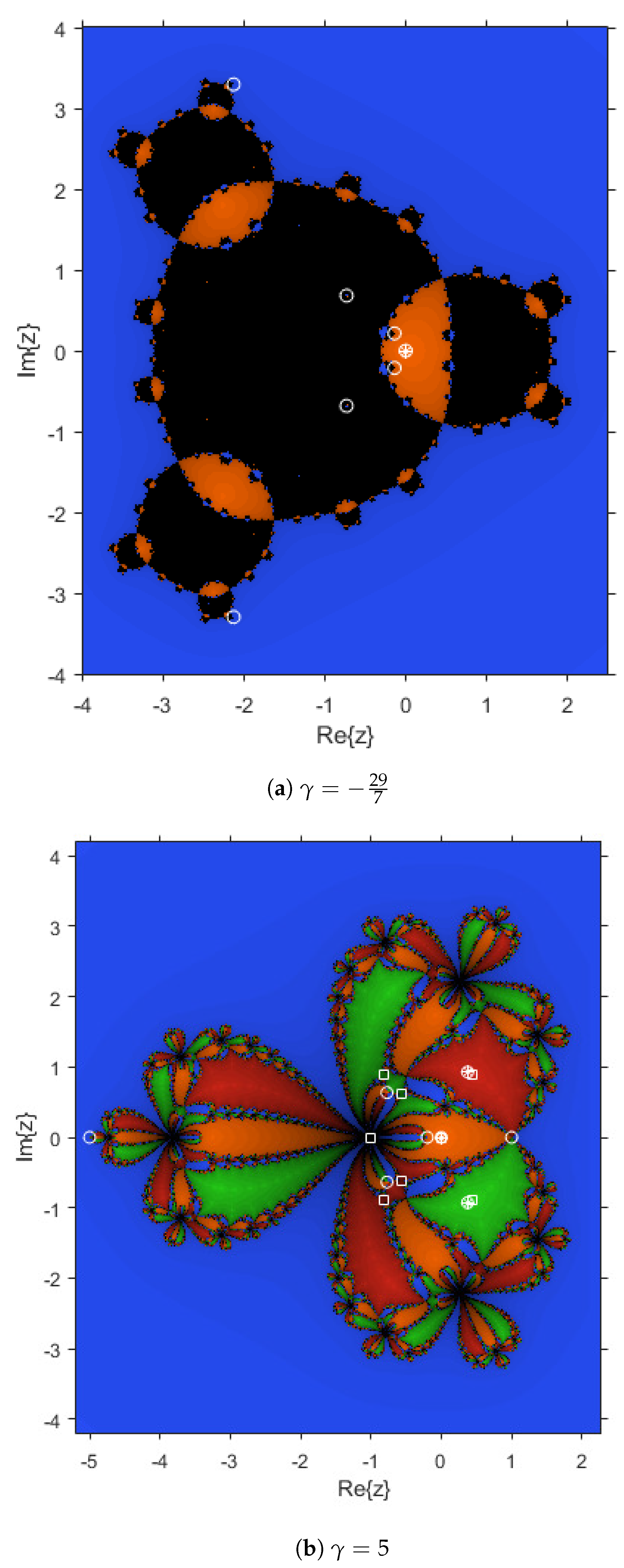
However, values such as γ = 10 + i , γ = 5 or γ = 29 7 present a dynamical plane with the same number of basins of attraction but with more complicated performance. We can see some of these dynamical planes in Figure 5a,b and Figure 6a. There are also parameter values for which the number of basins of attraction increases, for example, γ = 5 (Figure 6b). These cases should be avoided since our method may not converge to the roots and may end up converging to other points.

4. Numerical Experiments

In this section, we compare different iterative methods of the parametric family (2), solving two classical problems of applied mathematics: the Hammerstein integral equation and the Fisher partial derivative equation. We are going to use elements for the proposed class for which we have studied the dynamical plane because we want to verify that, although some of them have complicated dynamics, they can be methods that give good numerical results.
For the computational calculations, Matlab R2020b with variable precision arithmetics with 1000 digits of mantissa is used. From an initial estimation x ( 0 ) , the different algorithms calculate iterations until the stoping criterium x ( k + 1 ) x ( k ) < t o l is satisfied.
For the different examples and algorithms, we compare the approximation obtained, the norm of the function in the last iterate, the norm of the distance between the last two approximations, the number of iterations needed to satisfy the required tolerance, the computational time and the approximate computational convergence order (ACOC), defined by Cordero and Torregrosa in [16], which has the following expression:
p A C O C = ln ( x ( k + 1 ) x ( k ) 2 / x ( k ) x ( k 1 ) 2 ) ln ( x ( k ) x ( k 1 ) 2 / | x ( k 1 ) x ( k 2 ) 2 ) .

4.1. Hammerstein Equation

In this example, we consider the well-known Hammerstein integral equation (see [5]), which is given as follows:
x ( s ) = 1 + 1 5 0 1 F ( s , t ) x ( t ) 3 d t ,
where x C [ 0 , 1 ] , s , t [ 0 , 1 ] and the kernel F is
F ( s , t ) = ( 1 s ) t t s , s ( 1 t ) s t .
We transform the above equation into a finite-dimensional nonlinear problem by using the Gauss–Legendre quadrature formula given as 0 1 f ( t ) d t j = 1 7 ω j f ( t j ) , where the nodes t j and the weights ω j are determined for n = 7 by the Gauss–Legendre quadrature formula. In this case, the nodes and the weights are in Table 1.
By denoting the approximations of x ( t i ) by x i ( i = 1 , , 7 ), one gets the system of nonlinear equations:
5 x i 5 j = 1 7 a i j x j 3 = 0 ,
where i = 1 , , 7 and
a i j = w j t j ( 1 t i ) j i , w j t i ( 1 t j ) i < j .
Starting from an initial approximation x ( 0 ) = ( 1 , , 1 ) T and with a tolerance of t o l = 10 15 , we run the parametric family for different values of the parameter γ . The numerical results are shown in Table 2.
In all cases, we obtain as an approximation of the solution of Equation (25) the following vector x ( k + 1 ) = ( 1.0026875 , 1.0122945 , 1.0229605 , 1.0275616 , 1.0229605 , 1.0122945 , 1.0026875 ) T .
In the case of the Hammerstein integral equation, we see that the numerical results of the parametric family (2) for different values of γ are quite similar. The main difference observed between the methods is that the ACOC for γ = 0 is 4, and, for the rest of the methods, it is approximately 3. On the other hand, we note that the method with γ = 10 + i needs to perform a larger number of iterations than the rest of the methods to satisfy the required tolerance, so the time it takes to approximate the solution is also longer. Finally, taking into account the columns that measure the error of the approximation, that is, F ( x ( k + 1 ) ) 2 and x ( k + 1 ) x ( k ) 2 , we see that iterative methods that get lower errors are those associated with the parameters γ = 0 and γ = 2 . These results confirm the information obtained in the dynamical section.

4.2. Fisher Equation

In this second example, we are going to study the equation proposed in [17] by Fisher to model the diffusion process in population dynamics. The analytical expression of this partial derivative equation is as follows:
u t ( x , t ) = D u x x ( x , t ) + r u ( x , t ) 1 u ( x , t ) p , x [ a , b ] , t 0 ,
where D 0 is the diffusion constant, r is the level of growth of the species, and p is the carrying capacity.
In this case, we will study the Fisher equation for the values p = 1 , r = 1 , and D = 1 in the spatial interval [ 0 , 1 ] and with the initial condition u ( x , 0 ) = s e c h 2 ( π x ) and null boundary conditions.
We transform the problem we just described in a set of nonlinear systems by applying an implicit method of finite differences, providing the estimated solution in the instant t k from the estimated one in t k 1 . We denote the spatial step by h = 1 n x and the temporal step by k = T m a x n t , where T m a x is the final instant and n x and n t are the number of subintervals in x and t, respectively. Therefore, we define a mesh of the domain [ 0 , 1 ] × [ 0 , T m a x ] , composed of points ( x i , t j ) , as follows:
x i = 0 + i h , i = 0 , , n x , t j = 0 + j k , j = 0 , , n t .
Our objective is to approximate the solution of problem (26) in these points of the mesh, solving as many nonlinear systems as there are temporary nodes t j in the mesh. For this, we use the following finite differences:
u t ( x , t ) u ( x , t ) u ( x , t k ) k u x x ( x , t ) u ( x + h , t ) 2 u ( x , t ) + u ( x h , t ) h 2 .
We observe that, for the time step, we use first order backward divided differences and for the spatial step they are second order centered divided differences.
By denoting u i , j as the approximation of the solution at ( x i , t j ) , and, by replacing it in the Cauchy problem, we get the system
k u i + 1 , j + ( k h 2 2 k h 2 ) u i , j k h 2 u i , j 2 + k u i 1 , j = h 2 u i , j 1 ,
for i = 1 , 2 , , n x 1 and j = 1 , 2 , , n t . The unknowns of this system are u 1 , j , u 2 , j , , u n x 1 , j , that is, the approximations of the solution in each spatial node for the fixed instant t j .
In this example, we are going to work with the parameters T m a x = 10 , n x = 10 and n t = 50 . As we have said, it is necessary to solve as many systems as there are temporary nodes t j ; for each of these systems, we use the parametric family (2) to approximate its solution. Thus, starting from an initial approximation u i , 0 = s e c h 2 ( π x i ) , i = 0 , , n x , with a tolerance of 10 6 , we execute the parametric family for different values of γ so that we get Table 3.
In all cases, we obtain as an approximation of the solution of problem (26) the following vector x ( k + 1 ) = ( 0 , 4.32639 , 0.708718 , 0.853425 , 0.918847 , 0.93729 , 0.918847 , 0.853425 , 0.708718 , 0.432639 , 0 ) T .
In this case, it can seen that the results are very similar, although there are subtle differences. For example, the method when γ = 0 uses a smaller number of iterations than the rest to satisfy the required tolerance, although this does not make it much faster than the rest of the methods since the difference in time is seconds. On the other hand, if we look at the time column, we can see that there is a method that stands out for its slowness; this is the case of γ = 10 + i . Again, we note that the ACOC of the methods roughly match the theoretical predictions made throughout the article. Observing the columns of the errors, we find similar results as well and that, in this case, having a higher tolerance than in the first example, no great differences are observed in these results.

5. Conclusions

A parametric family of iterative methods for solving nonlinear systems is presented. The dynamical analysis of the class on quadratic polynomials is done in order to select the members of the family with better stability properties. We prove that there exist a wide set of real and complex values of the parameter for which the corresponding methods are stable. That is, the set of initial estimations converging to the roots is very wide.In particular, we have stated that those procedures with γ = 0 , γ = 1 , and γ = 2 are especially stable, although some other ones can also show similar dynamical properties. Two numerical examples related to Hammerstein’s equation and Fisher’s equation allow us to confirm the theoretical results corresponding to the convergence and the stability of the proposed class.

Author Contributions

The individual contributions of the authors are as follows: conceptualization, J.R.T.; writing—original draft preparation, E.G.V. and P.T.-N.; validation, A.C.; numerical experiments, E.G.V. and P.T.-N. All authors have read and agreed to the published version of the manuscript.

Funding

This research was supported by Ministerio de Ciencia, Innovación y Universidades PGC2018-095896-BC22 (MCIU/AEI/FEDER, UE).

Institutional Review Board Statement

Not applicable.

Informed Consent Statement

Not applicable.

Data Availability Statement

Not applicable.

Acknowledgments

The authors would like to thank the anonymous reviewers for their useful comments that have improved the final version of this manuscript.

Conflicts of Interest

The authors declare that there is no conflict of interest regarding the publication of this paper.

References

  1. Petković, M.S.; Neta, B.; Petković, L.D.; Dǔnić, J. Multipoint Methods for Solving Nonlinear Equations; Elserier: Amsterdam, The Netherlands, 2013. [Google Scholar]
  2. Amat, S.; Busquier, S. (Eds.) Advances in Iterative Methods for Nonlinear Equations; Springer: Cham, Switzerland, 2016. [Google Scholar]
  3. Chun, C.; Kim, Y. Several New Third-Order Iterative Methods for Solving Nonlinear Equations. Acta Appl. Math. 2010, 109, 1053–1063. [Google Scholar] [CrossRef]
  4. Maheshwari, A.K. A fourth order iterative method for solving nonlinear equation. Appl. Math. Comput. 2009, 211, 383–391. [Google Scholar] [CrossRef]
  5. Ortega, J.M.; Rheinboldt, W.C. Iterative Solution of Nonlinear Equations in Several Variables; Academic Press: Cambridge, MA, USA, 1970. [Google Scholar]
  6. Chicharro, F.I.; Cordero, A.; Torregrosa, J.R. Drawing dynamical and parameters planes of iterative families and methods. Sci. World J. 2013, 780153. [Google Scholar] [CrossRef] [PubMed]
  7. Hernández-Verón, M.A.; Magre nán, Ȧ.; Rubio, M.J. Dynamics and local convergence of a family of derivative-free iterative processes. J. Comput. Appl. Math. 2019, 354, 414–430. [Google Scholar]
  8. Chicharro, F.I.; Cordero, A.; Garrido, N.; Torregrosa, J.R. Generating root-finder iterative methods of second order: convergence and stability. Axioms 2019, 8, 55. [Google Scholar] [CrossRef] [Green Version]
  9. Lee, M.Y.; Kim, Y.I.; Neta, B. A generic family of optimal sixteenth-order multiple-root finders and their dynamics underlying purely imaginary extraneous fixed points. Mathematics 2019, 7, 562. [Google Scholar] [CrossRef] [Green Version]
  10. Chicharro, F.I.; Cordero, A.; Garrido, N.; Torregrosa, J.R. Generalized high-order classes for solving nonlinear systems and their applications. Mathematics 2019, 7, 1194. [Google Scholar] [CrossRef] [Green Version]
  11. Chicharro, F.I.; Cordero, A.; Garrido, N.; Torregrosa, J.R. Wide stability in a new family of optimal fourth-order iterative methods. Comput. Math. Methods 2019, 1, e1023. [Google Scholar] [CrossRef] [Green Version]
  12. Sharma, D.; Parhi, S.K. Local Convergence and Complex Dynamics of a Uni-parametric Family of Iterative Schemes. Int. J. Appl. Comput. Math. 2020, 6, 1–16. [Google Scholar] [CrossRef]
  13. Behl, R.; Bhalla, S.; Magreñán, Á.A.; Kumar, S. An efficient high order iterative scheme for large nonlinear systems with dynamics. Comput. Appl. Math. 2020, 113249. [Google Scholar] [CrossRef]
  14. Blanchard, P. Complex analitic dynamics on the Riemann splere. Bull. Am. Math. Soc. 1984, 11, 85–141. [Google Scholar] [CrossRef] [Green Version]
  15. Devaney, R.L. An Introduction to Chaotic Dynamical Systems; Addison-Wesley: Bostom, MA, USA, 1989. [Google Scholar]
  16. Cordero, A.; Torregrosa, J.R. Variants of Newton’s method using fifth-order quadrature formulas. Appl. Math. Comput. 2007, 190, 686–698. [Google Scholar] [CrossRef]
  17. Fisher, R.A. The wave of advance of advantageous genes. Ann. Eugen. 1937, 7, 353–429. [Google Scholar] [CrossRef] [Green Version]
Figure 1. Character of the roots of polynomial k ( t ) : (a) γ 1 , (b) γ 2 , (c) γ 3 , (d) γ 4 .
Mathematics 09 00086 g001
Figure 2. Parameter planes of O γ ( z ) .
Mathematics 09 00086 g002
Figure 3. Dynamical plane for γ = 0 and γ = 1 .
Mathematics 09 00086 g003
Figure 4. Dynamical plane for γ = 2 i and γ = 2 .
Mathematics 09 00086 g004
Figure 5. Dynamical planes of γ = 10 + i and γ = 5 .
Mathematics 09 00086 g005
Figure 6. Dynamical planes of γ = 29 7 and γ = 5 .
Mathematics 09 00086 g006
Table 1. Weights and nodes of the Gauss–Legendre quadrature.
iWeight ω i Abscissa t i
10.06474248310.0254460438
20.13985269570.1292344072
30.19091502520.2970774243
40.20897991850.5
50.19091502520.7029225757
60.13985269550.8707655928
70.06474248310.9745539561
Table 2. Hammerstein results for different parameters.
Parameter γ v F ( x ( k + 1 ) ) 2 x ( k + 1 ) x ( k ) 2 IterationACOCTime
05.40317 × 10 46 1.82600 × 10 184 43.9975338.0469
11.1060 × 10 20 7.36657 × 10 63 42.8588433.8594
−10 + i4.02251 × 10 45 3.70484 × 10 135 62.9880184.8594
29 / 7 1.73829 × 10 32 1.18363 × 10 97 52.9809544.0781
−58.18771 × 10 29 1.48807 × 10 86 52.9798746.2500
56.98712 × 10 28 9.02414 × 10 84 52.9722236.3281
2i5.87285 × 10 47 2.22194 × 10 141 52.9860635.3281
25.36968 × 10 17 8.93118 × 10 52 42.9350825.8750
Table 3. Fisher results for different parameters.
Parameter γ F ( x ( k ) ) 2 x ( k + 1 ) x ( k ) 2 IterationACOCTime
01.00166 × 10 8 1.12488 × 10 35 34.21099213.4219
11.9199 × 10 16 5.88036 × 10 50 42.99609248.7344
−10 + i8.08037 × 10 9 4.65282 × 10 26 53.01506352.6563
29 / 7 1.8002 × 10 7 2.00583 × 10 22 42.86978247.9844
−51.89574 × 10 19 2.9985 × 10 58 52.99569267.2969
52.4177 × 10 17 6.2774 × 10 52 52.99654275.7344
2i2.27659 × 10 11 1.96645 × 10 34 42.97846252.8438
29.67264 × 10 12 1.50906 × 10 35 43.00948231.2188
Publisher’s Note: MDPI stays neutral with regard to jurisdictional claims in published maps and institutional affiliations.

