Geographic Negative Correlation of Estimated Incidence between First and Second Waves of Coronavirus Disease 2019 (COVID-19) in Italy

Abstract

In this short communication, we investigate whether the intensity of the second wave of infection from SARS-CoV-2 that hit Italy in October–November–December 2020 is related to the intensity of the first wave, which took place in March–April 2020. We exploit the variation of the wave intensities across the 107 Italian provinces. Since the first wave has affected not only different regions, but also different provinces of the same region, at a heterogenous degree, this comparison allows useful insights to be drawn about the characteristics of the virus. We estimate a strong negative correlation between the new daily infections among provinces during the first and second waves and show that this result is robust to different specifications. This empirical result can be of inspiration to biologists on the nature of collective immunity underlying COVID-19.

1. Introduction

Italy, the first country in Europe after those in Asia, underwent a severe outbreak of Coronavirus Disease 2019 (COVID-19) during late winter 2020. The first detected cases were reported on 21 February 2020 in two Italian towns: Vo’ in the province of Padova, in the Veneto region, and Codogno, in the province of Lodi, in Lombardia. In the following weeks the epidemic spread quickly across Italy, but not uniformly. The most affected regions were Lombardia, Piemonte, Veneto and Emilia-Romagna in the north, and its neighbour central region, Marche.

In response to the epidemic spread, the Italian Government applied containment measures in three steps: first, some municipalities in Lombardia and Veneto went into quarantine (red zone); then, the entire Lombardia and some provinces in other northern and central regions (Veneto, Piemonte, Emilia-Romagna and Marche) were isolated from the rest of the country; finally, starting from 9 March, the whole of Italy was subjected to a hard, complete lockdown. Bertuzzo et al. modeled the spread of the COVID-19 epidemic in Italy in space and time, in which the progress of the wave of infections showed a spatial framework characterized by the radiation of the epidemic along highways and transportation infrastructures. Following similar studies, authors agree that Italy’s hard lockdown avoided the spread of the disease to the Centre and South of the peninsula [1,2,3]. As a result, and importantly for this study, in this first wave there was a large heterogeneity in the epidemic intensity of COVID-19 across regions and even across provinces of the same regions.

When in May and June 2020, the number of new daily cases and hospitalized ones drastically decreased, restrictive measures were weakened and then canceled. Thus, the first wave of COVID-19 in Italy displayed the standard phases: first, an initial outbreak phase with exponentially growing infections; second, a phase characterized by strong measures of social distancing; finally, a phase involving the reduction of the epidemic spread associated to weakened containment measures [4]. As a result, during summer people could travel and go on holiday, both at home and abroad, while the virus was not openly present, probably because of the seasonal characteristics of most respiratory diseases.

Since October, Italy has been experiencing a second severe wave of COVID-19 in which the reproduction number $R_t$ is changing over time heterogeneously across regions, although with some important common features, including a minimum value observed in mid-September, a mid-October peak and a decline during November [5]. The Italian government re-enforced, progressively, new restrictive measures starting from 13 October. Such measures were initially quite mild, but strengthened over time, until the establishment of “coloured zones”, yellow, orange and red, on 4 November, on the basis of 21 indexes highlighting the impact of the epidemic on the national health service. At the end of November this second wave experienced an evident decline in its intensity, with the reproduction number $R_t$ decreasing to values very close to the threshold of 1 and below almost everywhere [6]; however, in December the contagion curve visibly slowed its decay [7]. Clearly, even this second wave is characterized by a large heterogeneity of intensity across regions [7] and across provinces.

The main goal of this short communication is then to analyse, by exploiting the spatial COVID-19 incidence heterogeneity, whether there is a consistent link between the intensity of the first wave and the second wave. The epidemiological reasons why the COVID-19 epidemic has risen up again in autumn, and with such a strength, is not within the scope of this contribution. We provide evidence that the intensity of contagion in Italy during the first wave is geographically negatively correlated to the contagion during the second wave, and we show that this negative correlation is strong and statistically significant, not only for the worst-hit provinces in springtime, but also for larger areas and even for the whole country. Specifically, we study the incidence of SARS-CoV-2 infections between the two waves in Italy, referring to each of its 107 provinces. We take into consideration the number of daily new positive cases throughout the time starting from the first available data (24 February) to 28 December, subdividing such a time window into two parts: from 21 February to 16 July (first wave) and from 17 July to 28 December (second wave, not yet over). Importantly, in our analysis we control for regional effects, as lockdown policies have been implemented at that level; this way, exploiting the variation of provinces in the same region means the analysis is free from potential effects driven by different lockdown policies. Our results are robust to using different time windows to identify the two waves, as well as accounting for a different intensity of tracking when comparing the two waves.

The reason why we consider the rather unprecise number of daily new infections, and not, for example, the hospitalised or the deceased, is that, unfortunately, such parameters are not publicly available at the province level. The issue of undetected infections, thus, could become crucial in the evaluation of the incidence of the two outbreaks in same provinces. We also account for this possible issue in one of our robustness checks, in which we follow estimates in the literature [8,9,10,11] to differently weight the number of cases reported in the first wave and in the second wave: even in this case, the negative correlation of the intensity of the two waves remains strong.

2. Negative Correlation between Waves: Empirical Evidence

In this section, we document an important stylized fact about the intensity of the epidemic in Italy in the two waves. We provide evidence that the provinces in Italy that were more affected during the first wave in spring 2020, in terms of number of cases per 100 thousand people, were less affected in the second wave of fall 2020, and viceversa. While this negative correlation across waves is striking in some regions, for example Marche and Lombardia, it is strongly statistically significant when including all the regions and provinces.

Let us start by describing the data. We consider the number of official cases reported by the minister of health as a measure of epidemic intensity for each province (https://github.com/pcm-dpc/COVID-19). This is the only official statistics reported at the province level. As Italian provinces differ enormously in size, ranging from 4.3 million of residents in Rome to 83 thousand in Isernia, we scale the number of cases by population. The population by province was provided by the Italian statistical agency ISTAT and updated on the 31 December 2019 (All the results, figures and tables in this paper were produced using our own codes written in Matlab R2019b environment. The estimations were computed using the Matlab routine fitlm.m.).

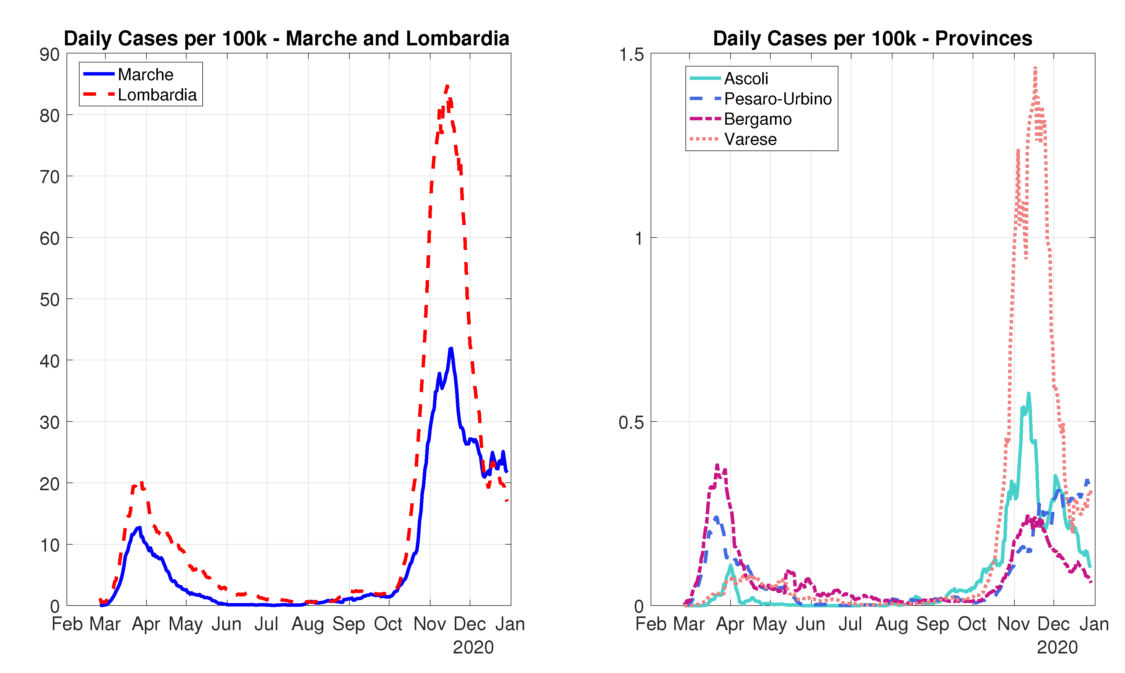
The left panel of Figure 1 displays the evolution of the daily number of cases in Marche (solid blue line) and Lombardia (red dashed line), two of the regions most affected by COVID-19. To eliminate the daily variations, we show a 7-day moving average. While the second wave appears to be more intense than the first one, there is quite strong heterogeneity across different provinces. In fact, in the right panel, we report the evolution of cases in Ascoli Piceno (dash-dotted light blue line) and Pesaro-Urbino (dotted dark blue line) for Marche, and in Bergamo (dashed dark red line) and Varese (solid orange line) for Lombardia. Notice that while Ascoli Piceno and Varese confirm the severity of the second wave with respect to the first one, on the contrary, Bergamo and Pesaro-Urbino experienced a second wave not particularly stronger than the first one. We would like to investigate the robustness of this negative correlation across waves.

Our strategy is to construct a measure of the intensity of the two waves across provinces. In our benchmark definition of a wave, we define $W_{ij}^{1\mathrm{st}}$ as the intensity of the first wave in province i in region j, measured as the total number of cases per 100 thousand people, from 24 February 2020, the first day in which data are available, to 16 July 2020. Similarly, we define $W_{ij}^{2\mathrm{nd}}$ as the intensity of the second wave from 17 July 2020 to 28 December 2020. While the date of separation between the two waves is arbitrary, it does not affect the main empirical facts, as we will show later.

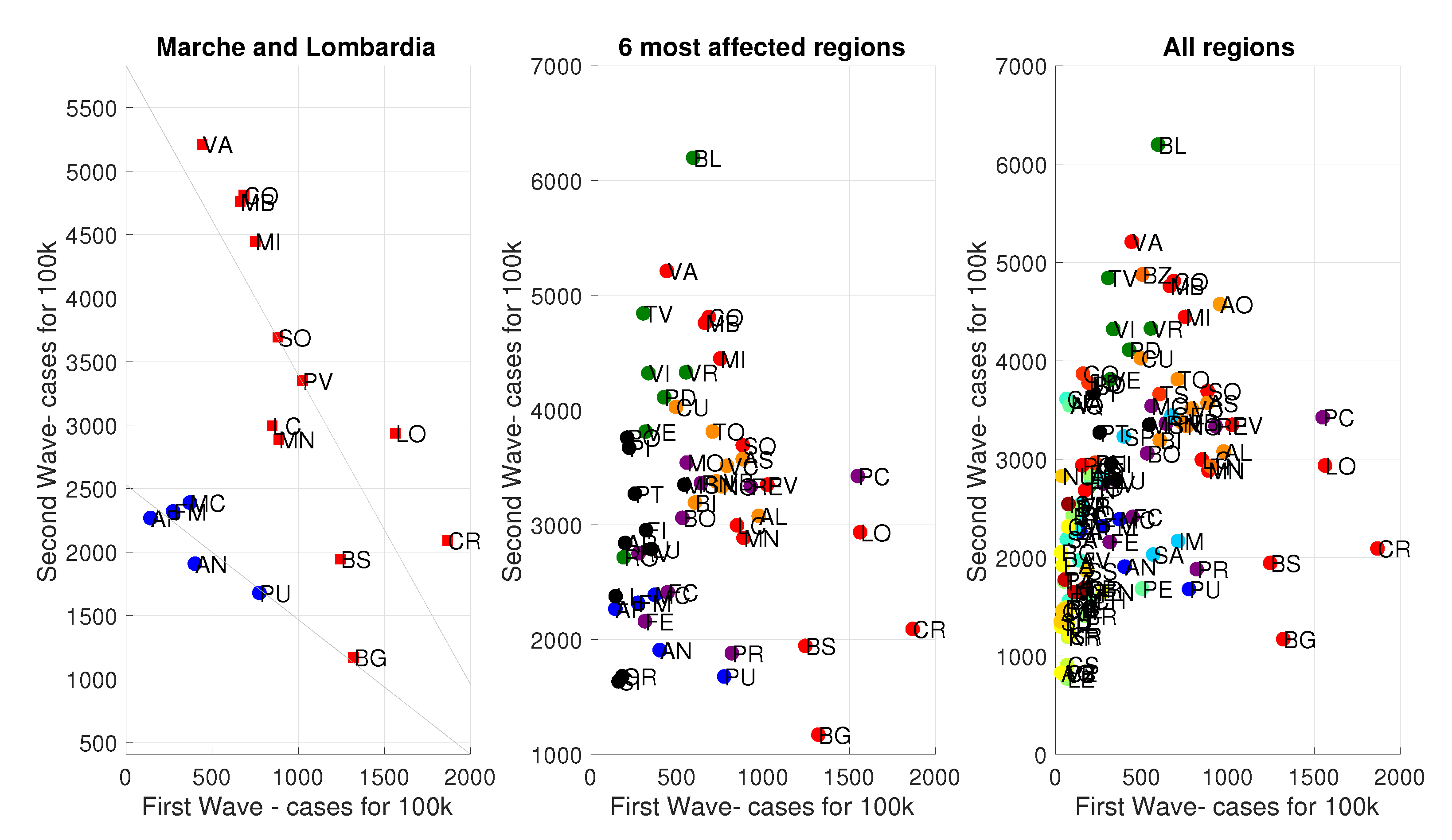
The left panel of Figure 2 shows the cross-correlation between the first and second wave intensities in the provinces of Marche (blue dots) and Lombardia (red squares). Conditioned on being in the same region, the provinces display a strong negative correlation of the two wave intensities, as illustrated by the regression lines (solid black lines).

One might wonder whether the negative correlation holds only for Marche and Lombardia. The central panel displays the same scatter plot for the 51 provinces in the 6 Italian regions most affected by the COVID-19 disease (Lombardia, Emilia-Romagna, Veneto, Piemonte, Marche and Toscana). These six regions account for 61% of the infections registered in Italy. Provinces in the same region share the same color and visually confirm the negative correlation across waves, conditioned on being in the same region. Finally, the right panel shows the scatter plot for all 107 provinces of the 20 Italian regions. As many southern regions have been less exposed to COVID-19 during springtime, these additional provinces lie in the bottom left region of the graph. The negative correlation remains strong, and, to formalize it, we will next move to a more formal regression analysis.

To formally confirm the existence of a negative correlation between wave intensities across the Italian provinces, we estimate the following regression:

$$\begin{array}{c}\hfill W_{ij}^{2\mathrm{nd}}={\alpha }_j+\beta W_{ij}^{1\mathrm{st}}+{\epsilon }_{ij},\end{array}$$

(1)

where ${\alpha }_j$ are region fixed-effects, i.e., intercepts that are allowed to vary across regions, and ${\epsilon }_{ij}$ are regression errors. Notice that here we are interested in only one slope parameter, $\beta$, which should therefore be interpreted as a country-wide relationship between wave intensities. As already hinted in the visual analysis above, it is important to control for region fixed effects because there is a strong heterogeneity in the degree by which COVID-19 has hit different areas in Italy. Controlling for being in the same region is crucial for two reasons. First, it allows for a more meaningful comparison of our effect of interest, that is the difference between the first and second wave in the same local area. Second, since lockdown policies have been implemented at the regional level, exploiting the variation of provinces in the same region means the analysis is free from potential effects driven by different lockdown policies.

Table 1. Regression results.

	(1)	(2)	(3)	(4)	(5)
	All Regions	Top 6 Regions	Marche and Lombardia	Different Sample	Tracking Factor
$\widehat{\beta }$	−0.941 ***	−0.860 **	−2.29 ***	−0.872 **	−0.297 ***
std. error	0.361	0.432	0.493	0.374	0.114
p-value	0.010	0.050	0.000	0.022	0.010
Observations	107	51	17	107	107
Degree of Freedom	86	44	14	86	86
Adjusted $R^2$	0.54	0.32	0.65	0.53	0.54
Region Fixed Effects	Yes	Yes	Yes	Yes	Yes
All regions	Yes	No	No	Yes	Yes
Top 6 regions	No	Yes	No	No	No
Lombardia and Marche	No	No	Yes	No	No
Break between waves	No	No	No	Yes	No
Tracking Factor	No	No	No	No	Yes

Note: This table displays the estimates of the regression in Equation (1) with different specifications. Regression (1) considers all 107 provinces. Regression (2) considers the 6 Italian regions most affected by the COVID-19 disease (Lombardia, Emilia-Romagna, Veneto, Piemonte, Marche and Toscana). Regression (3) considers only provinces in Marche and Lombardia. Regression (4) ignores the data during the summer. Regression (5) scales the cases in the first wave by a factor of 19 and the cases in the second waves by a factor of 6, to account for the infections that remain undetected due to the inadequate (or impossible) tracking strategies. ** denotes statistical significance at 5 percent, while *** denotes statistical significance at 1 percent.

reports our estimation results. The first specification (1) includes all the 107 Italian provinces. The negative correlation between the two waves is strong and statistically significant at 1%. The adjusted $R^2$ is quite large, and equal to 0.54: this is not surprising as the regions’ fixed effects help the fit. The strong negative correlation is confirmed when reducing the sample size. The second specification (2) includes only the 51 provinces in the 6 Italian regions most affected by COVID-19, consistently with what is shown in the central panel of Figure 2. The size and precision of the estimate for our parameter of interest, $\beta$, are quite unaffected, which confirms that including the southern regions does not alter the nature of the correlation across waves. The third specification (3) includes only Lombardia and Marche, consistently with what is shown in the left panel of Figure 2. The negative correlation, as expected, is even stronger and strongly significant. The fourth specification (4) uses a different definition of first and second wave, which excludes summer. In this case, the first wave is measured as the number of cases in the first three months of our observation, that is from 24 February to 23 May, while the second wave is measured as the number of cases in the last three months of our time window, that is from 2 September to 28 December. Hence, we have excluded the summer period in which the epidemic had a very low incidence. The negative correlation is basically unaffected by eliminating the summer period. Finally, the fifth specification (5) scales the number of cases in the first and second waves by different multiplying factors aiming to control for the possibility of different tracking strategies which might have affected the number of official cases. However, even when accounting for this possibility, the strong negative correlation between waves remains large and highly significant.

It is important to justify the use of these different tracking factors to scale the daily new positive in the two waves. During the first wave, the testing capacity of countries, and of Italy in particular, was insufficient and largely conditioned, at least in the early stages, by focusing on individuals related to China or to Chinese people. This point was highlighted by Li et al. [8], who inferred the proportion of early infections in China that went undetected and their contribution to virus spread worldwide. They estimated that around 86% of cases were undocumented before travel restrictions were put in place. Additionally, Bommel and Vollmer [9] estimated that up to 16 March, the detected new daily positive were just 6% of the total amount of infections, whereas, up to 31 March, this percentage became 9% of the total. In a different work, Kuniya [10] assumed that the detected cases are only 1% to 10% of the total infection cases, while Phypps et al. [11], using a backcasting approach coupled with Monte Carlo methods, estimated that the true number of people infected across 15 countries for which reliable data were available was 18.2 (5–95% CI: 11.9–39.0) times greater than the reported number of cases. In particular, the true number of cases exceeds that of detected cases by factors that range from 1.7 (95% CI: 1.1–3.6) for Australia to 35.6 (95% CI: 23.2–76.3) for Belgium. From the above considerations, due to the lack of specific information for Italian data, we assume that the official number of daily new positives should be multiplied by factors ranging from 10 up to 32. In the figures that follow, we used the value of 19 as an arbitrary choice that is reasonably located in the middle of the interval [10, 32], but our simulations show that significance is not affected by any other value in the assumed range. For the second wave, we have to consider two windows of time: from mid July to mid October approximately, when the contact tracing was similar to the reality, with the spread of the virus being low, and from the second half of October to now (29 December), when any possibility of tracing was lost due to the huge amount of new daily positive cases. For the first part of the observation, we consider the results of the massive testing of the population of Vo’ (Veneto) during March 2020, showing that 42.5% (95% CI: 31.5–54.6%) of the confirmed SARS-CoV-2 infections were asymptomatic (they did not have symptoms at the time of swab testing nor did they develop symptoms afterwards, i.e., they were truly asymptomatic, not pre-symptomatic) [12]. For the second window, we refer in part to the results of the 3-day mass screening (20–22 November) that was performed in the Bolzano-Alto Adige autonomous province, to which the 63.9% of the population adhered [13]. The asymptomatic cases were 22.5% of the total positive cases referred to 22 November, the last day of the testing. If we extend this percentage to the population of the different Italian regions, we obtain a mean 33% of undetected cases in Italy, ranging from the minimum 22.5% of Bolzano to the maximum 58% of the autonomous province of Trento. Considering that a certain amount of undetected cases could be included in the almost 40% of citizens who did not adhere to the screening, we assume that the undetected proportion may be as high as 50%.Unfortunately, due to the huge number of cases across all Italian regions, at the end of October, the close contacts of positive people, if not symptomatic, were just quarantined without any testing, apart from the leaving swab after 14 or 21 days. This suggests that for each positive case, there may have been at least 7 or 8 undetected cases, in particular, among asymptomatic children or adults. For similar reasons as those inspiring the multiplicative factor used for the first wave data, we assume that official numbers in the second wave should be multiplied by a factors ranging from 2 to 8. We chose an intermediate value of 6, but our simulations confirm that significance remains for any other value in the assumed range.

Region-Specific Estimation

Our main result concerns an estimated negative correlation between the intensities of the first and second wave for the Italian provinces. By exploiting the variation across provinces within each region, as displayed in regression (1), we are able to estimate our parameter of interest, $\beta$, which is a country-wide estimate of such correlation. A different approach would be to estimate such a correlation for each region. This approach has the drawback that, since in many regions there are only very few provinces, the resulting estimates might be rather imprecise. Nevertheless, in this section, we conduct that exercise and we compute the region-specific estimation of the correlation of the wave intensity ${\beta }_j$ resulting from the following regression:

$$\begin{array}{c}\hfill W_{ij}^{2\mathrm{nd}}={\alpha }_j+{\beta }_j{W}_{ij}^{1\mathrm{st}}+{\epsilon }_{ij}.\end{array}$$

(2)

Table 2. Region-specific estimation.

	${\mathit{\beta }}_{\mathit{j}}$	Std. Error	p-Value	Adjusted ${\mathit{R}}^2$	Observations
Lombardia	−2.43	0.59	0.002	0.59	12
Marche	−1.06	0.42	0.09	0.56	5
Veneto	5.52	2.14	0.05	0.49	7
Emilia-Romagna	0.60	0.54	0.29	0.03	9
Piemonte	−1.19	0.70	0.14	0.21	6
Toscana	2.55	2.00	0.23	0.06	10

Note: this table reports the estimates of the parameter ${\mathit{\beta }}_{\mathit{j}}$ in regression (2), first column, for the 6 regions that were most affected by COVID-19, the corresponding standard error, p-value, and Adjusted ${\mathit{R}}^2$ of the regression.

reports the estimates of ${\beta }_j$, their standard error and p-value, together with the Adjusted $R^2$ for the top 6 most affected regions (Lombardia, Marche, Veneto, Emilia-Romagna, Piemonte, and Toscana). There are two main points to highlight. First, the estimates are quite heterogenous across regions: while some regions, such as Lombardia and Marche, display a strong negative correlation, Veneto exhibits a different pattern. Second, because of the small number of provinces within a region, the region-specific parameters are not precisely estimated, as it can be seen by the quite large standard deviations and the rather low $R^2$. Accordingly, while Piemonte and Toscana, respectively, display a negative and positive point estimate, the uncertainty regarding such a parameter is too large to draw any inference.

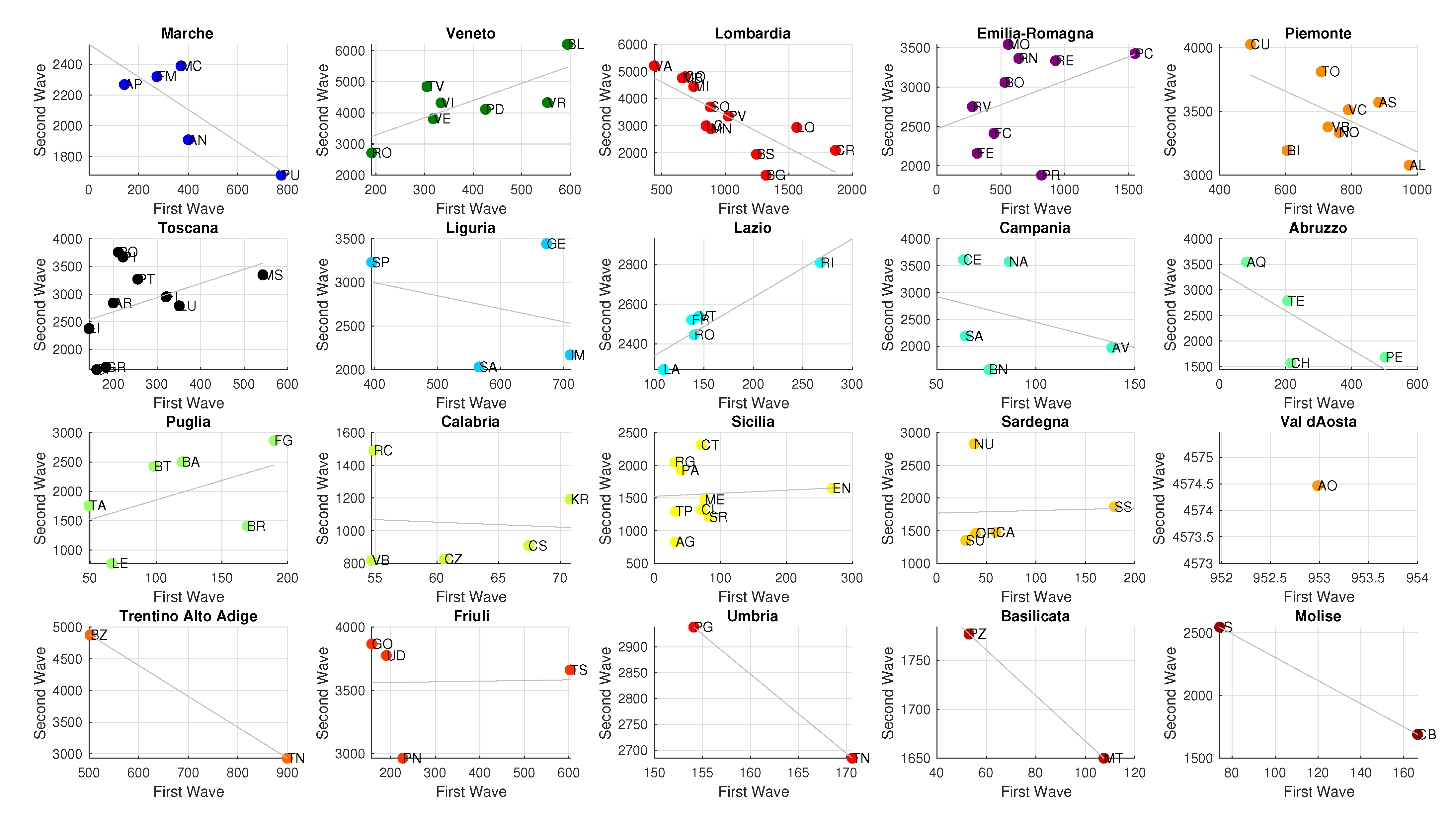
Obviously, we can estimate the parameters for 19 of the 20 Italian regions (because Val d’Aosta has only one province, regression (2) cannot be estimated for that region), thus obtaining a distribution of the region-specific slope parameters. We now report some statistics of that distribution: the average ${\beta }_j$ is equal to −1.30, the median ${\beta }_j$ is equal to −1.06, while the standard deviation of the distribution is 4.99. These statistics confirm the fact that, although there is quite a large heterogeneity across regions, the overall number of regions with negative correlations is quite high, thus rationalizing the results we obtained for the country-wide estimates. In Figure 3, we display the relationship between the first and second wave intensities for each of the twenty regions: the solid black line corresponds to the regression line, whose slope is the estimated parameter ${\beta }_j$.

3. Discussion

The Italian provinces that were worst hit by COVID-19 in Spring 2020 (Bergamo, Brescia, Cremona, Lodi, Piacenza, Pesaro-Urbino) appear to be the least hit in the second wave in fall and viceversa (Milano, Monza, Como, Varese, Ascoli Piceno, ...). How can this negative correlation be explained? One hypothesis is biological. It is likely that the worst hit provinces in the first wave have acquainted a collective immunity due to several factors that are being revealed by studies on the biological features of SARS-CoV-2. It is known, for example, that in some towns of Val Seriana (province of Bergamo) 40–50% of the population developed antibodies against the virus after the spring outbreak [14]. Prevalence in the entire province of Bergamo reached 38.5% [15]. Despite how long these antibodies remain present in the blood, cellular mediated immunity could protect the population. Fontanet [16] reports that the first epidemic wave (not only in Italy) resulted in higher levels of immunity across the population than measured through cross-sectional antibody surveys. Grifoni et al. [17] detected SARS-CoV-2-reactive CD4+ T cells in 40–60% of unexposed individuals, suggesting crossreactive T cell recognition between coronaviruses responsible of commonly circulating colds and SARS-CoV-2. However, whether T cells can prevent SARS- CoV-2 infection or protect against severe disease is still an open question [18]. There is also a second hypothesis explaining the different rate of infection in the same areas and it is rather sociological. People having undergone a dramatic situation in earlier times could have developed a much higher sensibility to avoid risks than people living in areas where COVID-19 did not spread before. During summer, containment measures were relaxed but people who experienced contagion and deaths in spring were probably more careful than people who did not. On the other hand, Lombardy as a whole region, was hit in spring and is being hit even now, highlighting the strength of this new coronavirus and suggesting that we cannot let our guard down. Certainly, after the first epidemic wave, the population living in central and southern Italy was much more susceptible, since there were few areas in which any kind of collective immunity had been developed to slow down the virus boost. We conclude with the following observation due to Villa [19,20] on the basis of reported data from ISPI [21]. The total number of people truly infected by SARS-CoV-2 since February 2020 in Italy, by 28 December, is estimated to be about 6.7 million, two thirds of which occurred during the second epidemic wave. This number corresponds to slightly more than 11% of the population, a proportion that is far from herd immunity. On 11 and 18 December, the FDA issued an Emergency Use Authorisation (EUA) for the Pfizer–Biontech and Moderna vaccines. Results of phase III of the AstraZeneca and Pfizer–Biontech vaccines have recently been published in [22,23]. On 8 and 14 December, the United Kingdom and the United States, respectively, began their vaccine campaigns. The EMA recommended granting a conditional marketing authorisation for the Pfizer–Biontech vaccine on 21 December and EU member countries began their vaccination campaigns on 27 December 2020. With the optimism that comes from science, we think we are almost at the end of the line and that 2021 could be the year when we get out of the pandemic, hopefully, worldwide.