Determination of Aircraft Cruise Altitude with Minimum Fuel Consumption and Time-to-Climb: An Approach with Terminal Residual Analysis

Abstract

A pandemic situation of COVID-19 has made a cost-minimization strategy one of the utmost priorities for commercial airliners. A relevant scheme may involve the minimization of both the fuel- and time-related costs, and the climb trajectories of both objectives were optimized to determine the optimum aircraft cruise altitude. The Hermite-Simpson method among the direct collocation methods was employed to discretize the problem domain. Novel approaches of terminal residual analysis (TRA), and a modified version, m-σ TRA, were proposed to determine the goals. The multi-objective cruise altitude (MOCA) was different by 2.5%, compared to the one statistically calculated from the commercial airliner data. The present methods, TRA and m-σ TRA were powerful tools in finding a solution to this complex problem. The value σ also worked as a transition criterion between a single- and multi-objective climb path to the cruise altitude. The exemplary MOCA was determined to be 10.91 and 11.97 km at σ = 1.1 and 2.0, respectively. The cost index (CI) varied during a flight, a more realistic approach than the one with constant CI. With validated results in this study, TRA and m-σ TRA may also be effective solutions to determine the multi-objective solutions in other complex fields.

1. Introduction

The outbreak of COVID-19 made the year 2020 the worst year in the history of the airline industry, with a net loss of 84.3 billion dollars [1]. The official reports from the Bureau of Transportation Statistics (BTS) of U.S. already confirmed a net loss of 5.2 billion and 11 billion dollars in the first [2] and second [3] quarters, respectively, of the year 2020. Revenue passenger kilometer (RPK) fell by 55% and cargo & mail ton-kilometer (CTK) by 16.8%, and the year 2021 is also expected to be unfavorable [1]. Although Ref. [1] notes that the overall prediction of the performance of the airline industry is favorable in 2021, the end of this pandemic is still unpredictable. Amidst a harsh pandemic environment, tight cost management became even more crucial, and the authors propose a rational, cost-minimizing approach. Since fuel expenditure is almost a quarter (23.7%) of the total operating cost (TOC) [1], and the time of arrival is also as essential as fuel costs, the focus of our study is on the minimization of both the fuel consumption (FC) and the time of travel (TT).

The optimization of FC and TT indeed is one of the major priorities in the literature as multi-objective [4,5,6,7,8,9,10] and single-objective [11,12,13,14,15] studies using various methods of Gauss Pseudo-spectral method [16] (sometimes accompanied by Chebyshev direct method [4]), energy-state [11,12], genetic algorithm [5], particle swarm [10], direct collocation methods [17,18], and statistical approach [9]. The optimization of each phase in a flight profile, consisting of the climb, cruise, and descent, had distinct merits for improvements. First, the cruise phase contributes the most to the TOC, even more for a long-range flight. Aircraft under the descent phase uses all of their potential and kinetic energy for deceleration, but the optimization is primarily for safety [19,20]. During the climb phase, optimized ascension protocols such as continuous climb operations (CCOs) yield a considerable reduction in fuel consumption [21,22]. The authors chose the climb phase for multi-objective optimization because of its potential for further optimization [9,12].

Overall, the main objective of this study is to minimize both FC and TT in conjunction with the climb phase. In this case, TT became the time-to-climb (TTC) to describe the time spent to ascend to the desired optimum cruise altitude. From the perspective of aerodynamics, cruising at higher altitudes reduces the aerodynamic drag and increases cruise speed at a given thrust, but there is extra fuel consumption for ascension [23]. Cruising at a lower altitude implies more aerodynamic drag and lower aircraft speed, which resulted in increased TT. An optimally determined cruise altitude would save both fuel and time, potentially achievable by optimizing the aircraft performance during the ascending phase. This study does not adapt the conventional approach of total cost minimization involving constant cost index (CI) throughout a flight path [3,5,7] but shows that CI changes over the course of the climb path. Moreover, wind shear conditions were not considered, and only conventional International Standard Atmosphere (ISA) conditions were used. This ISA model is equivalent to the 1976 US standard atmosphere model [24], and hence the atmosphere model used in the present study was named ”1976 US atmospheric model”. This study presents a distinctive method, effectively determining the optimum cruise altitude of a generic supersonic aircraft using residual analysis arguments, incorporating two minimizing objectives, FC and TTC. The rationale for the use of supersonic jet data was given in the next paragraph and Section 4.

The contents start with a brief description of the indirect method and explain the difficulties involved in finding the analytic solution of complex problems in Section 2.1. Section 2.2 describes the direct methods, which had gained popularity with the increase in computing power in recent decades. The study justifies the use of direct methods over indirect methods. There are several direct methods such as the Gauss-Lobatto [25] and the Gauss Pseudo-spectral method [16], but the Hermite-Simpson method was chosen. The procedure with the chosen method for the discretization of the problem domain in Section 2.2 as well. The calculated cruise altitude result was compared to the statistically derived result from subsonic, commercial airplanes in Ref. [9]. The present study intended to calculate the cruise altitude of an aircraft by optimizing the climb trajectory in three-dimensional thrust-Mach-altitude space. Such data in the literature using subsonic commercial aircraft [9,22] was available only in stage-wise aerodynamic data having single column data at each flight stage, and hence, the authors used supersonic jet data [12,26] with boundary conditions set for subsonic operations. The details about the models were described in Section 2.3, and auxiliary models and novel methods used in this paper were noted in Section 2.4, Section 2.5 and Section 2.6. The optimum climb trajectories were obtained for each targeted objective, minimum FC and TTC. Then, the results (Section 3) were presented followed by discussions (Section 4) and conclusion (Section 5).

2. Methods

The following Section 2.1 and Section 2.2 describe the general formulation of the optimal control problem (OCP).

2.1. Optimal Control in Continuous-Time Domain

In general, the formulation of continuous-time optimal control problem with no path constraints on the states or the control variables and fixed initial and final time $t_0$ and $t_E$ can be defined as follows:

$$J=\mathsf{\Phi }\left(x\left(t_E\right)\right)+{{\displaystyle \int }}_{t_0}^{t_E}L\left(x\left(t\right),u\left(t\right),t\right) dt$$

(1)

where the control vector trajectory $u:\left[t_0,t_E\right]\subset ℝ\mapsto {ℝ}^{n_u}$ is usually minimized in the performance index $J:\left[t_0,t_E\right]\times {ℝ}^{n_x}\times {ℝ}^{n_u}\times ℝ\mapsto ℝ$. Equation (1) is subject to:

$$\dot{x}\left(t\right)=f\left(x\left(t\right), u\left(t\right),t\right),x\left(t_0\right)=x_0$$

(2)

where $\left[t_0,t_E\right]$ is the time interval of the problem domain, $x:\left[t_0,t_E\right]\mapsto {ℝ}^{n_x}$ is the state vector, $\mathsf{\Phi }:{ℝ}^{n_x}\times ℝ\mapsto ℝ$ is a terminal cost function, $L:{ℝ}^{n_x}\times {ℝ}^{n_u}\times ℝ\mapsto ℝ$ is an intermediate cost function, and $f:{ℝ}^{n_x}\times {ℝ}^{n_u}\times ℝ\mapsto {ℝ}^{n_x}$ is a vector field. This formulation is expressed in the Bolza form where Equation (2) describes the dynamics of the system with the corresponding initial conditions. Here, $\mathsf{\Phi }\left(x\left(t_E\right)\right)$ is the Mayer term and $L\left(x\left(t\right),u\left(t\right),t\right)$ is the Lagrange term.

When constraints are involved, a time dependent Lagrange multiplier vector function $\lambda :\left[t_0, t_E\right]\mapsto {ℝ}^{n_x}$, also known as co-state, is introduced to define an augmented performance index $\overline{J}$, which is defined as:

$$\overline{J}=\mathsf{\Phi }\left(x\left(t_E\right)\right)+{{\displaystyle \int }}_{t_0}^{t_E}\left(L\left(x\left(t\right),u\left(t\right),t\right)+{\lambda }^T\left(t\right)\left[f\left(x\left(t\right),u\left(t\right),t\right)-\dot{x}\right]\right) dt.$$

(3)

The Hamiltonian function $\mathscr{H}$ then is defined as:

$$\mathscr{H}\left(x\left(t\right),u\left(t\right),\lambda \left(t\right),t\right)=L\left(x\left(t\right),u\left(t\right),t\right)+{\lambda }^T\left(t\right)f\left(x\left(t\right),u\left(t\right),t\right),$$

(4)

which can re-write Equation (3) as:

$$\overline{J}=\mathsf{\Phi }\left(x\left(t_E\right)\right)+{{\displaystyle \int }}_{t_0}^{t_E}\left(\mathscr{H}\left(x\left(t\right),u\left(t\right),\lambda \left(t\right),t\right)- {\dot{\lambda }}^T\left(t\right)\dot{x}\right) dt.$$

(5)

When time $t_0$ and $t_E$ are fixed, an infinitesimal variation in $u\left(t\right)$, $x\left(t\right)$, and $\overline{J}$ can be considered which are denoted as $\delta u\left(t\right)$, $\delta x\left(t\right)$, and $\delta \overline{J}$. Such can be formulated as:

$$\begin{array}{c}\delta \overline{J}={\left[\left(\frac{\partial \mathsf{\Phi }}{\partial \mathrm{x}}-{\lambda }^T\right)\delta x\left(t\right)\right]}_{t=t_E}+{\left[{\lambda }^T\delta x\left(t\right)\right]}_{t=t_0}\\ \hspace{1em}\hspace{1em}\hspace{1em}\hspace{1em}\hspace{1em}\hspace{1em}\hspace{1em}\hspace{1em}\hspace{1em}\hspace{1em}\hspace{1em}\hspace{1em}\hspace{1em}\hspace{1em}\hspace{1em}\hspace{1em}\hspace{1em}\hspace{1em}+{{\displaystyle \int }}_{t_0}^{t_E}\left(\left(\frac{\partial \mathscr{H}}{\partial x}+ {\dot{\lambda }}^T\right)\delta x\left(t\right)+\left(\frac{\partial \mathscr{H}}{\partial u}\right)\delta u\left(t\right)\right) dt.\end{array}$$

(6)

The Lagrange multipliers $\lambda :\left[t_0, t_E\right]\mapsto {ℝ}^{n_x}$ can arbitrarily be chosen to make $\delta x\left(t\right)$ and $\delta x\left(t_E\right)$ coefficient equal to zero. Hence the multipliers chosen are:

$${\dot{\lambda }}^T\left(t\right)=-\frac{\partial \mathscr{H}}{\partial x},$$

(7)

$${\lambda }^T\left(t_E\right)={\frac{\partial \mathsf{\Phi }}{\partial \mathrm{x}}|}_{t=t_E}.$$

(8)

The chosen multipliers change the expression for $\overline{J}$. When the initial state is fixed at $\delta x\left(t_0\right)=0$:

$$\overline{\delta }\overline{J}={\int }_{t_0}^{t_E}\left[\left(\frac{\partial \mathscr{H}}{\partial u}\right)\delta u\right] dt,$$

(9)

where the stationarity condition for the minimum at $\delta \overline{J}=0$ becomes:

$$\frac{\partial {\mathscr{H}}^T}{\partial u}=0.$$

(10)

Equations (2), (7), (8) and (10) are the necessary conditions in the first order for a minimum of $J$. Equations (7) and (8) are known as the adjoint equation, describing the co-states, and the transversality conditions, describing the initial states. These are necessary optimality conditions defining a two-point boundary value problem, useful for finding analytic solutions to certain types of optimal control problems. They also are used to find solutions in general cases using numerical algorithms. Further details are described in Refs. [27,28,29].

Definition 1.

(Terminal constraints).The above formulation can be given a set of terminal constraints defined as:

$$\psi \left(x\left(t_E\right),t_E\right)=0,$$

(11)

where$\psi :{ℝ}^{n_x}\times ℝ\mapsto {ℝ}^{n_{\psi }}$is in a vector form, variational analysis shows that Equations (2), (7) and (10) become necessary conditions for a minimum of$J$with the following terminal condition:

$${{\left(\frac{\partial {\psi }^T}{\partial x}+\frac{\partial {\psi }^T}{\partial x}\zeta -\lambda \right)}^T|}_{t_E}\delta x\left(t_E\right)+{\frac{\partial \psi }{\partial t}+\frac{\partial {\psi }^T}{\partial t}\zeta +\mathscr{H}|}_{t_E}\delta t_E=0,$$

(12)

where$\zeta \in {ℝ}^{n_{psi}}$is Lagrange multiplier for the terminal constraint,$\delta t_E$is the infinitesimal variation in$t_E$, and$\delta x\left(t_E\right)$is the infinitesimal variation in$x\left(t_E\right)$.

Definition 2.

(Pontryagin’s maximum principle).The adaptation of inequality constraints coupled to the input variables in optimal control problems is common under realistic conditions [30]. The input variable$u$then is restricted within the admissible compact region$\Omega$, which is defined as:

$$u\left(t\right)\in \Omega .$$

(13)

In this case, Equations (2), (7) and (8) become necessary conditions, and stationarity condition of Equation (10) is replaced with:

$$\mathscr{H}\left(x^{*}\left(t\right), u^{*}\left(t\right), {\lambda }^{*}\left(t\right), t\right)=\underset{u\left(t\right)\in U}{\max }\mathscr{H}\left(x^{*}\left(t\right), u^{*}\left(t\right), {\lambda }^{*}\left(t\right), t\right),$$

(14)

for all admissible $u\left(t\right)$. The superscript * denotes the optimal variables. The above, Pontryagin’s maximum principle, Hamiltonian $\mathscr{H}$ must be maximized over all admissible $u\left(t\right)$ for optimal values of the state and co-state variables.

Definition 3.

(Path constraints).The problem domain in practical applications usually restricts the state and control trajectories where a set of constraints have to be satisfied within a time interval $\left[t_0,t_E\right]$. The constraint in the trajectory is given as:

$$E\left(x\left(t\right),u\left(t\right),t\right)\le 0,$$

(15)

where$E:{ℝ}^{n_x}\times {ℝ}^{n_u}\times \left[t_0,t_E\right]\mapsto {ℝ}^{n_P}$. Additionally, equality constraints can be imposed at some intermediate point in time$t_e$,$t_0\le t_e\le t_E$. These interior point constraints can be expressed as:

$$D\left(x\left(t_e\right),t_e\right)=0,$$

(16)

where$D:{ℝ}^{n_x}\times ℝ\mapsto {ℝ}^{n_q}$. Further details are available in Ref. [31].

Definition 4.

(Singular arcs).In singular arc problems, the matrix${\partial }^2\mathscr{H}/\partial u^2$becomes singular with external arcs satisfying Equation (10). In this case, the optimality of the singular arc should be validated [31,32]. Usually, Hamiltonian function$\mathscr{H}$becomes linear in at least one of the control variables for certain practical cases. This causes the control not to be determined with the state and co-state by Equation (10), but by the condition where the time derivative of $\partial \mathscr{H}/\partial u$is zero along the singular arc. In such cases, supplementary conditions called the generalized Legendre-Clebsch conditions must be identified:

$${\left(-1\right)}^k\frac{\partial }{\partial u}\left[\frac{d^{2k}}{d{t}^{2k}}\frac{\partial \mathscr{H}}{\partial u}\right]\ge 0, k=0,1,2,\dots .$$

(17)

The computational difficulty involved in singular arc problems is the non-unique control variables. The inequality constraint domains, especially, have complications of:

• An unknown number of constrained sub-arcs at the initial stage of formulation.
• Unidentified locations of the junction points where the transition from the constrained to the unconstrained (and vice versa) occur.
• Possible discontinuity of both the control variables $u$ and the adjoint variable $\lambda$ at the junction points which is related to the dissatisfaction of boundary conditions.

2.2. Direct Transcription Method

The complexity involved in solving the indirect methods questions its robustness. The direct methods, on the other hand, have advantages over indirect methods that good initial and any co-state guesses are not compulsory, making them robust by having a broad range for convergence even without optimally derived conditions and undetermined switching structure. Linear interpolation discretizes a continuous solution to a set of equations with state and control variables to solve the differential equations. As a result, this transforms an OCP into nonlinear programming (NLP) problem where the exact solution of OCP, having an infinite number of state and control variable combinations, is approximated to a finite number.

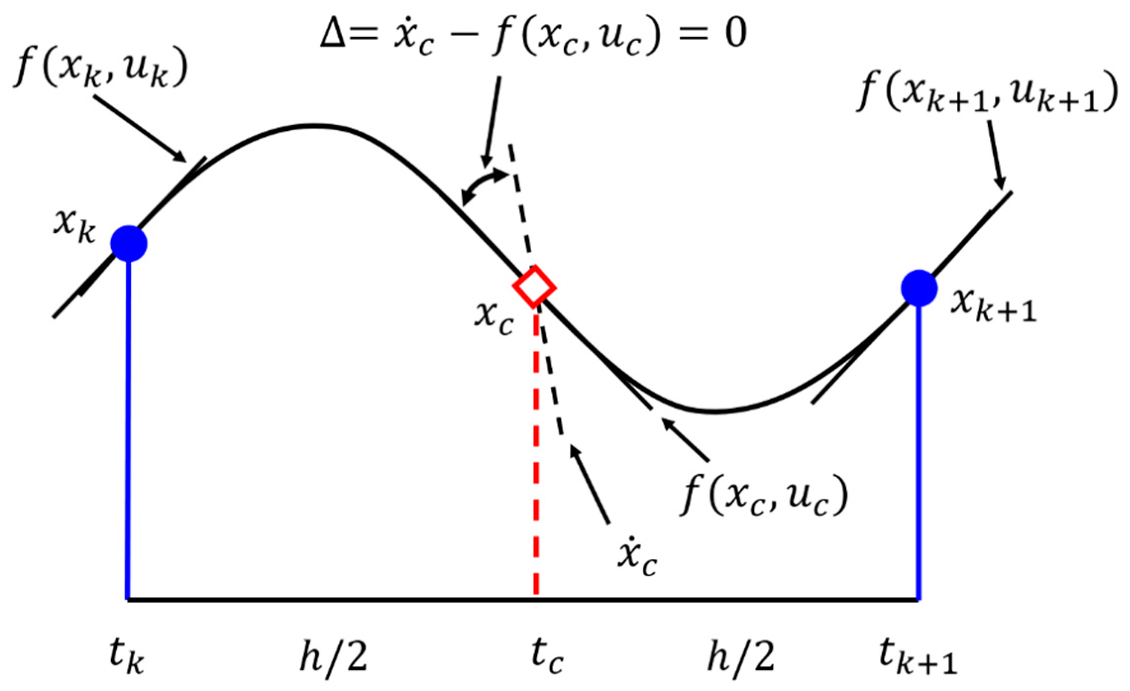
The typical methods are direct shooting, direct multiple shooting, and direct collocation. A direct collocation method is robust in problems with small perturbations, which is suitable for aircraft trajectory optimization. The present study uses the Hermite-Simpson methods with cubic polynomials to define the state trajectories and a piece-wise linear function for the control [18] (Figure 1). This method places the collocation points at the centers of the intervals and imposes constraints on the dynamic equations during the discretization process.

First, time $t_E$ is discretized into N intervals as:

$${\mathrm{t}}_0=0\le t_1\le t_2\dots \le t_k\le t_{k+1}\le \dots \le t_N=t_E.$$

(18)

The states between $t_k$ and $t_{k+1}$ can be expressed in the form of cubic polynomial as:

$$x\left(t\right)=a_{k,0}+a_{k,1}t+a_{k,2}{t}^2+a_{k,3}{t}^3,$$

(19)

which gives a derivative form of:

$$\dot{x}\left(t\right)=a_{k,1}+2a_{k,2}t+3a_{k,3}{t}^2,$$

(20)

where $a_{k,0}$, $a_{k,1}$, $a_{k,2}$, and $a_{k,3}$ are coefficients of the polynomial approximation in $k^{t}h$ interval. Since the collocation point is the midpoint of the interval:

$$t_{k,c}=\frac{t_k+t_{k+1}}{2}.$$

(21)

The values of the state and its derivatives are independent to the shifting of the interval from $\left[t_k,t_{k+1}\right]$ to $\left[0,h\right]$ with $h=t_{k+1}-t\_k$, time interval should be shifted. Let $x\left(0\right)=x_k$, $x\left(h\right)=x\_\left(k+1\right)$, $\dot{x}\left(0\right)={\dot{x}}_k$, and $\dot{x}\left(z\right)={\dot{x}}_{k+1}$, and combining Equations (19) and (20) gives:

$$\left[\begin{array}{c}x\left(0\right)\\ \dot{x}\left(0\right)\\ x\left(h\right)\\ \dot{x}\left(h\right)\end{array}\right]=\left[\begin{array}{cccc}1& 0& 0& 0\\ 0& 1& 0& 0\\ 1& h& h^2& h^3\\ 0& 1& 2z& 3h^2\end{array}\right]\left[\begin{array}{c}{a}_{k,0}\\ a_{k,1}\\ a_{k,2}\\ a_{k,3}\end{array}\right].$$

(22)

In the inverse form gives:

$$\left[\begin{array}{c}{a}_{k,0}\\ a_{k,1}\\ a_{k,2}\\ a_{k,3}\end{array}\right]=\left[\begin{array}{cccc}1& 0& 0& 0\\ 0& 1& 0& 0\\ -\frac{3}{h^2}& -\frac{2}{h}& \frac{3}{h^2}& -\frac{1}{h}\\ \frac{2}{h^3}& \frac{1}{h^2}& -\frac{2}{h^3}& \frac{1}{h^2}\end{array}\right]\left[\begin{array}{c}x\left(0\right)\\ \dot{x}\left(0\right)\\ x\left(h\right)\\ \dot{x}\left(h\right)\end{array}\right].$$

(23)

The substitution of coefficients $\left[a_{k,0}, a_{k,1}, a_{k,2}, a_{k,3}\right]$ into Equations (19) and (20) allows for the computation of the collocation points as:

$$\begin{gathered} x_c\left(t\right)=x\left(\frac{h}{2}\right) \\ =\frac{1}{2}\left(x_k\left(t\right)+x_{k+1}\left(t\right)\right)+\frac{h}{8}\left[f\left(x_k\left(t\right), u_k\left(t\right)\right)-f\left(x_{k+1}\left(t\right), u_{k+1}\left(t\right)\right)\right]. \end{gathered}$$

(24)

In the time-derivative form, the points in the center of the interval is given by:

$${\dot{x}}_c\left(t\right)=\dot{x}\left(\frac{h}{2}\right)=-\frac{3}{2h}\left(x_k-x_{k+1}\right)-\frac{1}{4}\left[f\left(x_k,u_k\right)\right].$$

(25)

The above equation depends on the states and control at the intervals. Appropriate values of both state and controls should be chosen for the collocation points to represent the correct physics of the system. The control at the collocation point is given by:

$$u_c=\frac{u_k+u_{k+1}}{2}.$$

(26)

A defect ${\Delta }_k$ is then described as follows:

$$\begin{array}{ll}{\Delta }_k& ={\dot{x}}_c-f\left(x_c,u_c\right)\\ & =-\frac{3}{2h}\left(x_k-x_{k+1}\right)-\frac{1}{4}\left[f\left(x_k,u_k\right)+f\left(x_{k+1},u_{k+1}\right)\right]-f\left(x_c,u_c\right)\\ & =-\frac{3}{2h}\left[\left(x_k-x_{k+1}\right)+\frac{h}{6}\left[f\left(x_k,u_k\right)+4f\left(x_c,u_c\right)+f\left(x_{k+1},u_{k+1}\right)\right]\right].\end{array}$$

(27)

State constraints then are redefined as:

$${\Delta }_k=\left[\left(x_k-x_{k+1}\right)+\frac{h}{6}\left[f\left(x_k,u_k\right)+4f\left(x_c,u_c\right)+f\left(x_{k+1},u_{k+1}\right)\right]\right].$$

(28)

The last term in the above expression is implicit Hermite integration of the system dynamics which is used to solve nonlinear functions. Here, the NLP solver would select $\left[x_k,u_k,x_{k+1},u_{k+1}\right]$ to minimize $\Delta$ to zero for convergence of the solution.

The cost function now can be defined using numerical integration schemes. When trapezoid method is chosen, the cost function is written as:

$$J\left(u\right)=\mathsf{\Phi }\left(x\left(t_E\right)\right)+{{\displaystyle \int }}_{t=0}^{t_E}L\left(t,x\left(t\right),u\left(t\right)\right) dt.$$

(29)

Using trapezoid integration along the interval:

$$J_{NLP}=\mathsf{\Phi }\left(x_N\right)+\frac{1}{2}{\displaystyle \sum }_{k=1}^{N-1}\left(L\left(t_{k+1},x_{k+1},u_{k+1}\right)+L\left(t_k,x_k,u_k\right)\right)\left(t_{k+1}-t_k\right).$$

(30)

For a special case with linear quadratic regulator and evenly discretized time points at the intervals $h$, the resultant equation is expressed as:

$$J_{NLP}=\mathsf{\Phi }\left(x_N\right)+\frac{1}{2}{\displaystyle \sum }_{k=1}^{N-1}\left(x_{k+1}^T{Q}_1{x}_{k+1}+u_{k+1}^T{Q}_2{u}_{k+1}+x_k^T{Q}_1{x}_k+u_k^T{Q}_2{u}_k\right)h.$$

(31)

In general, the problem formulation using NLP in the OCP can be rewritten as:

$$\underset{x_k,u_k}{\min }\left(\mathsf{\Phi }\left(x_N\right)+\frac{1}{2}{\displaystyle \sum }_{k=1}^{N-1}\left(x_{k+1}^T{Q}_1{x}_{k+1}+u_{k+1}^T{Q}_2{u}_{k+1}+x_k^T{Q}_1{x}_k+u_k^T{Q}_2{u}_k\right)h\right).$$

(32)

where $Q_1$ and $Q_2$ are linear quadratic regulators, and Equation (32) is subjected to:

$${\Delta }_k=[\left(x_k-x_{k+1}\right)+\frac{h}{6}\left[f\left(x_k,u_k\right)+4f\left(x_c,u_c\right)+f\left(x_{k+1},u_{k+1}\right)\right]=0,$$

(33)

with constraints on states and controls defined as:

$$\begin{gathered} u_{min}\le u_k\le u_{max}, \\ {x}_{min}\le x_k\le u_{max}, \\ {C}_{eq}\left(x_k,u_k\right)=0, \\ C\left(x_k,u_k\right)=0, \end{gathered}$$

(34)

where $C_{eq}$ and $C$ represent equality and inequality constraints, respectively.

The procedure described in this section was used to solve the problem in this study which is already implemented in the MATLAB-compatible toolbox ICLOCS2 [34], where nonlinear problems were solved with interior point NLP solver IPOPT [35].

2.3. Aircraft Model

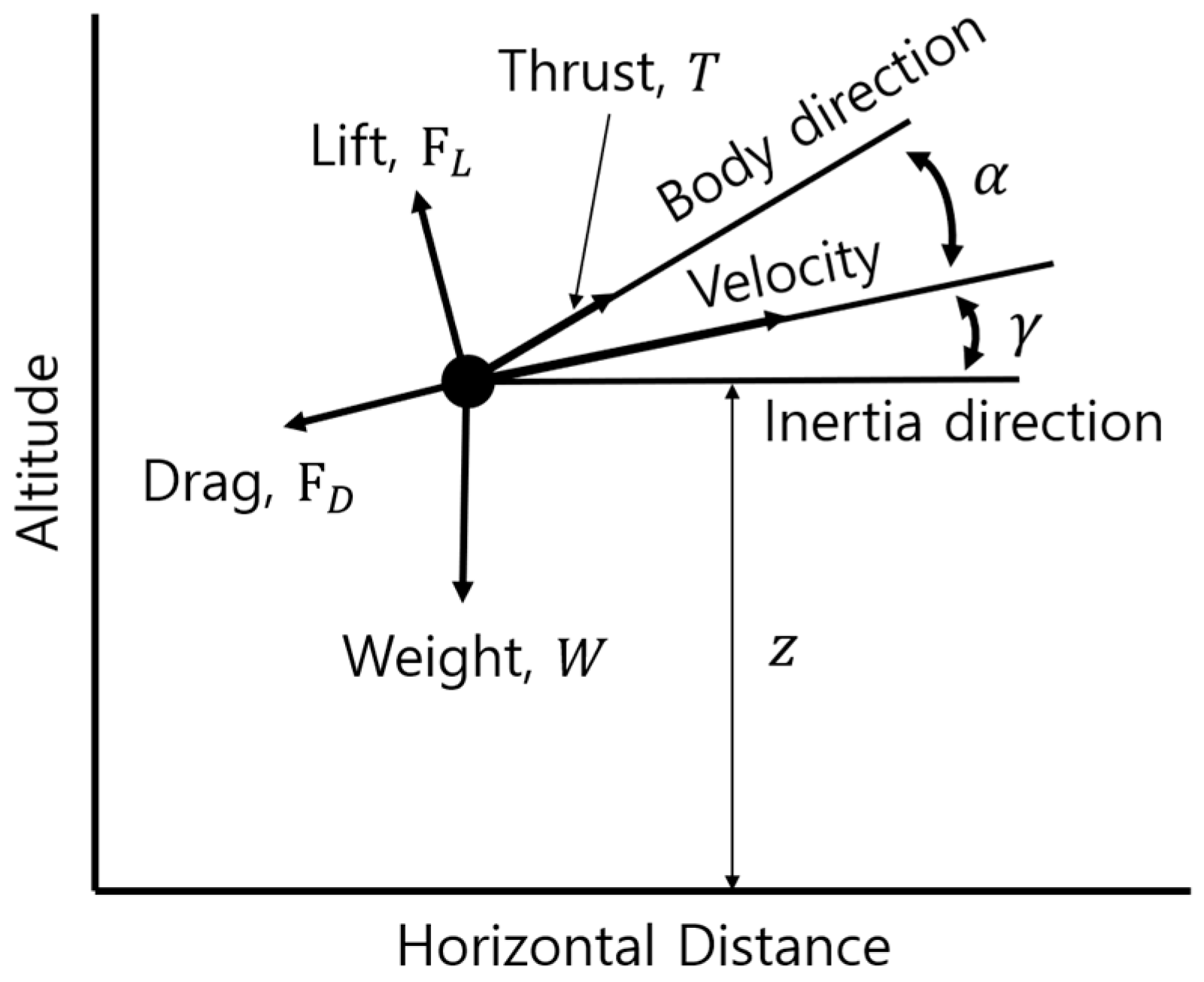
The multi-objective in this study is the achievement of both minimum FC and TTC to reach the optimum cruise altitude. To achieve these objectives, the climb path to the desired altitude should be optimized. First, the equation of motion (EOM) (Figure 2) in point-mass approximation adopted from Ref. [36] can be written as follows:

$$\dot{V}=\frac{\left(T\left(M,z\right)\cos \alpha -F_D\right)}{m}-\frac{\epsilon }{r_t^2}\sin \gamma ,$$

(35)

$$\dot{\gamma }=\frac{T\left(M,z\right)\sin \alpha +F_L}{mV}+\left[\frac{V}{r_t}-\frac{\epsilon }{v{r}_t^2}\cos \gamma \right],$$

(36)

$$\dot{z}=V\sin \gamma ,$$

(37)

$$\dot{W}=-\frac{T\left(M,z\right)}{I_{sp}},$$

(38)

where $V$ is airspeed, $T$ is thrust, $M$ is Mach number, $F_D$ is drag, $F_L$ is lift, $W$ is weight, a product of mass $m$ and gravitational acceleration $g_0$, $\epsilon$ is the gravitational constant, $r_t$ is the sum of the radius of the Earth $R_e$ and the altitude $z$, $\gamma$ is the flight path angle, and $\alpha$ is angle of attack. They are subject to initial conditions of $V\left(t_i\right)=V_i$, $\gamma \left(t_i\right)={\gamma }_i$, $z\left(t_i\right)=z_i$, and $m\left(t_i\right)=m_i$, where $t_i$ is the initial time. The aerodynamic properties of the aircraft are approximated with functions of $\alpha$:

$$F_L=qS{C}_{L_{\alpha }}\alpha ,$$

(39)

$$F_D=qS\left(C_{D_0}+\eta C_{L_{\alpha }}{\alpha }^2\right),$$

(40)

where $q=\rho V^3/2$ denotes the dynamic pressure, $S$ is the aerodynamic reference area, $\eta$ is the efficiency factor ($0\le \eta \le 1$). Both $C_{L_{\alpha }}$ and $C_{D_0}$ are the slope coefficients of lift and zero-lift drag which are dependent on the Mach number, $M$, in most cases.

The objectives in this study are minimum FC and TTC. Hence, the cost functions for each objective are given as Equations (41) and (42), respectively:

$$\underset{x\left(t\right),u\left(t\right),t_E}{\min }-m\left(t_E\right),$$

(41)

$$\underset{x\left(t\right),u\left(t\right),t_E}{\min }{t}_E,$$

(42)

The altitudes as boundary conditions were given in 1 km interval and hence the $z\left(t_E\right)$ was given a range between 1000 m to 21,000 m with an interval of 1 km. The boundary conditions and the constants were given as:

$z\left(0\right)=0 \left[\mathrm{m}\right],$	$V\left(0\right)=129 \left[\mathrm{m}/\mathrm{s}\right],$	$\gamma \left(0\right)=0 \left[\mathrm{deg}\right],$	$m\left(0\right)=19,050 \left[\mathrm{kg}\right],$
$V\left(t_E\right)=295 \left[\mathrm{m}/\mathrm{s}\right],$	$\gamma \left(t_E\right)=0 \left[\mathrm{deg}\right],$	$S=49.24 \left[{\mathrm{m}}^2\right],$
$\epsilon =3.99\times {10}^{14} \left[{\mathrm{m}}^3/{\mathrm{s}}^2\right],$	$I_{sp}=1600 \left[\mathrm{s}\right],$	$g_0=9.81 \left[\mathrm{m}/{\mathrm{s}}^2\right],$	$R_e=6,378,145 \left[\mathrm{m}\right],$

with the bounds on the variables, given as:

$0\le z\le 21,000 \left[\mathrm{m}\right],$	$5\le V\le 1200 \left[\mathrm{m}/\mathrm{s}\right],$	$40\le \gamma \le 40 \left[\mathrm{deg}\right],$
$100\le m\le 20,000 \left[\mathrm{kg}\right],$	$-20\le \alpha \le 20 \left[\mathrm{deg}\right],$	$0\le t_E\le 600 \left[\mathrm{s}\right],$

where the accuracy criteria for the numerical solution was given as

Table 1. Accuracy criteria for the numerical solution.

Accuracy Criteria
	$\mathit{z} \left[\mathbf{m}\right]$	$\mathit{V} \left[\mathbf{m}/\mathbf{s}\right]$	$\mathit{\gamma } \left[\mathbf{d}\mathbf{e}\mathbf{g}\right]$	$\mathit{m} \left[\mathbf{k}\mathbf{g}\right]$
${\zeta }_{tol}$	1	0.5	1	1
${\chi }_{g_{tol}}$	1	0.5	1	1
${\zeta }_{tol}$	Maximum absolute local error
${\chi }_{g_{tol}}$	Maximum local constraint violation

.

The thrust and aerodynamic data should be defined either with the experimental data or highly refined simulation data, preferably using computational fluid dynamics with direct numerical simulation (DNS) [37] sometimes coupled with linear interaction analysis (LIA) [38], or large eddy simulation (LES) [39] for an accurate description of an object moving in a compressible fluid like air. Simulation data describing the macroscopic motion of the aircraft [26,40] also are valuable resources. In the present study, typical supersonic aircraft aerodynamic profiles employed from Refs. [12,26] were used and reproduced in

Table 2. Thrust as a function of altitude $z$ and Mach number $M$ from Ref. [12] adjusted by Ref. [41] for Aircraft 1.

	Thrust, T $({10}^3 \mathbf{l}\mathbf{b}$$, 4.5\times {10}^3$N)
Mach No., $\mathit{M}$	Altitude, z $({10}^3 \mathbf{f}\mathbf{t}, 0.3\times {10}^3$m)
	0	5	10	15	20	25	30	40	50	70
0	24.2	24	20.3	17.3	14.5	12.2	10.2	5.7	3.4	0.1
0.2	28	24.6	21.1	18.1	15.2	12.8	10.7	6.5	3.9	0.2
0.4	28.3	25.2	21.9	18.7	15.9	13.4	11.2	7.3	4.4	0.4
0.6	30.8	27.2	23.8	20.5	17.3	14.7	12.3	8.1	4.9	0.8
0.8	34.5	30.3	26.6	23.2	19.8	16.8	14.1	9.4	5.6	1.1
1.0	37.9	34.3	30.4	26.8	23.3	19.8	16.8	11.2	6.8	1.4
1.2	36.1	38	34.9	31.3	27.3	23.6	20.1	13.4	8.3	1.7
1.4	36.1	36.6	38.5	36.1	31.6	28.1	24.2	16.2	10	2.2
1.6	36.1	35.2	42.1	38.7	35.7	32	28.1	19.3	11.9	2.9
1.8	36.1	33.8	45.7	41.3	39.8	34.6	31.1	21.7	13.3	3.1

and

Table 3. Lift and drag coefficients as a function of angle of attack $\alpha$ and Mach number $M$ from Ref. [12] for Aircraft 1.

Aerodynamic Parameters	Mach No.,
	0	0.4	0.8	0.9	1.0	1.2	1.4	1.6	1.8
$C_{L_{\alpha }}$	3.44	3.44	3.44	3.58	4.44	3.44	3.01	2.86	2.44
$C_{D_0}$	0.013	0.013	0.013	0.014	0.031	0.041	0.039	0.036	0.035
$\eta$	0.54	0.54	0.54	0.75	0.79	0.78	0.89	0.93	0.93

, where adjustments were made by Ref. [41] with linear interpolation to fill in the ”missing” data. According to the authors in Ref. [26], the aircraft is a generic-type supersonic interceptor.

A second aircraft model (

Table 4. Thrust as a function of altitude $z$ and Mach number $M$ from Ref. [12] for Aircraft 2.

	Thrust, T $({10}^3 \mathbf{l}\mathbf{b}$$, 4.5\times {10}^3$N)
Mach No., $\mathit{M}$	Altitude, z $({10}^3 \mathbf{f}\mathbf{t}, 0.3\times {10}^3$m)
	0	5	15	25	35	45	55	65	75	85	95	105
0	23.3	20.6	15.4	9.9	5.8	2.9	1.3	0.7	0.3	0.1	0.1	0.1
0.4	22.8	19.8	14.4	9.9	6.2	3.4	1.7	1.0	0.5	0.3	0.1	0.1
0.8	24.5	22.0	16.5	12.0	7.9	4.9	2.8	1.6	0.9	0.5	0.3	0.2
1.2	29.4	27.3	21.0	15.8	11.4	7.2	3.8	2.7	1.6	0.9	0.6	0.4
1.6	29.7	29.0	27.5	21.8	14.7	10.5	6.5	3.8	2.3	1.4	0.8	0.5
2.0	29.9	29.4	28.4	26.6	21.2	14.0	8.7	5.1	3.3	1.9	1.0	0.5
2.4	29.9	29.2	28.4	27.1	25.6	17.2	10.7	6.5	4.1	2.3	1.2	0.5
2.8	29.8	29.1	28.2	26.8	25.6	20.0	12.2	7.6	4.7	2.8	1.4	0.5
3.2	29.7	28.9	27.5	26.1	24.9	20.3	13.0	8.0	4.9	2.8	1.4	0.5

and

Table 5. Lift and drag coefficients as a function of angle of attack α and Mach number M from Ref. [11] for Aircraft 2.

Aerodynamic Parameters	Mach No.,
	0	0.4	0.8	0.9	1.0	1.2	1.4	1.6	1.8
$C_{L_{\alpha }}$	3.44	3.44	3.44	3.58	4.44	3.44	3.01	2.86	2.44
$C_{D_0}$	0.013	0.013	0.013	0.014	0.031	0.041	0.039	0.036	0.035
$\eta$	0.54	0.54	0.54	0.75	0.79	0.78	0.89	0.93	0.93

) was then employed using the same approach to compare the possible difference between two aircraft models. The same cost functions and altitude range as Aircraft 1 were given with slightly different boundary and constraint conditions as shown below:

$z\left(0\right)=0 \left[\mathrm{m}\right],$	$V\left(0\right)=129 \left[\mathrm{m}/\mathrm{s}\right],$	$\gamma \left(0\right)=0 \left[\mathrm{deg}\right],$	$m\left(0\right)=16,329.3 \left[\mathrm{kg}\right],$
$V\left(t_E\right)=295 \left[\mathrm{m}/\mathrm{s}\right],$	$\gamma \left(t_E\right)=0 \left[\mathrm{deg}\right],$	$S=46.45 \left[{\mathrm{m}}^2\right],$
$\epsilon =3.99\times {10}^{14} \left[{\mathrm{m}}^3/{\mathrm{s}}^2\right],$	$I_{sp}=2800 \left[\mathrm{s}\right],$	$g_0=9.81 \left[\mathrm{m}/{\mathrm{s}}^2\right],$	$R_e=6,378,145 \left[\mathrm{m}\right],$

with the bounds on the variables, given as:

$0\le z\le 21,000 \left[\mathrm{m}\right],$	$5\le V\le 1200 \left[\mathrm{m}/\mathrm{s}\right],$	$40\le \gamma \le 50 \left[\mathrm{deg}\right],$
$100\le m\le 20,000 \left[\mathrm{kg}\right],$	$-20\le \alpha \le 20 \left[\mathrm{deg}\right],$	$0\le t_E\le 600 \left[\mathrm{s}\right],$

Refs. [12,26] mentions that both models were based on typical supersonic interceptors. To the best of the authors’ knowledge, supersonic interceptors have two types: one is heavy, long-range, and the other is lightweight, short-range, and the authors speculated that Aircraft 1 belonged to the former, and Aircraft 2 for the latter for having different initial mass (19,050 compared to 16,329.3 kg) and maximum thrust (205.65 compared to 134.55 kN). The authors note that the cruise altitude cannot be the same for all aircraft and may vary depending on the aircraft model. The results of the aircraft model 2 and the effects of such differences were presented and discussed in Section 4.5.

2.4. Atmospheric Model

For a realistic approach to the problem, a 1976 US atmospheric model [24] was used. This semi-empirical model effectively describes the atmospheric conditions around an aircraft at all altitudes and made the mathematical approach in this study more realistic. The formula for the model is given as:

$$T_M=T_b+L_b\left(z-z_b\right),$$

(43)

$$P=\{\begin{array}{c}{P}_b{e}^{\left[\frac{g_0{M}_A\left(z-z_b\right)}{R{T}_b}\right]}, L_b=0; \\ P_b{\left[\frac{T_b}{T_b+L_b\left(z-z_b\right)}\right]}^{\left[\frac{g_0{M}_A}{R{L}_b}\right]}{L}_b\ne 0;\end{array}$$

(44)

$$\rho =\frac{P}{R_{sp}T},$$

(45)

where $T_M$ is the molecular temperature, $T_b$ is the base temperature at each atmospheric level, $L_b$ is the base temperature lapse rate, $z$ is altitude, $z_b$ is the base altitude at each atmospheric level, $P$ is atmospheric pressure, $P_b$ is the base pressure at each atmospheric level, $g_0$ is gravitational acceleration, $R$ is universal gas constant, $M_A$ is molar mass of Earth’s air, $\rho$ is the density of air, and $R_{sp}$ is the specific gas constant of air. The atmospheric level, and the necessary boundary and parameter values are given in

Table 6. 1976 US atmosphere model: boundary and parameter values from Ref. [24].

Atmospheric Level	Altitude Range (km)	${\mathit{b}}^{*}$	${{\mathit{z}}_{\mathit{b}}}^{†}$	${\mathit{P}}_{\mathit{b}} {\left(\mathbf{P}\mathbf{a}\right)}^{‡}$	${\mathit{T}}_{\mathit{b}} {\left(\mathbf{K}\right)}^{\S }$	${\mathit{L}}_{\mathit{b}} {\left(\mathbf{K}/\mathbf{k}\mathbf{m}\right)}^{\Vert }$
Troposphere	0–11	0	0	101325	288.15	−6.5
Tropopause (Stratosphere I)	20–32	1	11	22,632.06	216.65	0.0
Stratosphere II	20–32	2	20	5474.89	216.65	+1.0
Stratosphere III	32–47	3	32	868.02	228.65	+2.8
Stratopause (Mesosphere I)	47–51	4	47	110.91	270.65	0
Mesosphere II	51–71	5	51	66.94	270.65	−2.8
Mesosphere III	71–84.9	6	71	3.96	214.65	−2.0
―	―	7	84.852	0.37	186.87	―

Note: $*$, Interval (Layer) Number; $†$, Base Geopotential Altitude Above Mean Sea Level (MSL); $‡$, Base Static Pressure; $\S$, Base Temperature; $\Vert$, Base Temperature Lapse Rate per Kilometer of Geopotential Altitude.

.

2.5. B-Spline Curve

The optimum trajectory solutions of each target objectives, minimum FC and TTC, were generated with an altitude interval of 1000 m, and B-spline was selected for the plotting of the curve connecting the property values at the end of the climb. B-spline is the general form of the Bézier spline which builds parametric curves around the polynomial expressions [42]. When a knot vector is $B={\beta }_0,{\beta }_1,\dots ,{\beta }_k,$ and control points $w_0, \dots ,w_n$ are defined where $B$ is a non-decreasing sequence with ${\beta }_i\in \left[0,1\right]$, the basis functions are defined as below:

$$N_{i,o}\left(\beta \right)=\{\begin{array}{c}1,if {\beta }_i\le \beta \le {\beta }_{i+1} and {\beta }_i<{\beta }_{i+1};\\ 0,otherwise;\end{array}$$

(46)

where $j=1,2,\dots ,w.$ The B-spline curve then is defined as:

$$N_{i,j}\left(\beta \right)=\frac{\beta -{\beta }_i}{{\beta }_{i+j}-{\beta }_i}{N}_{i,j-1}\left(\beta \right)+\frac{{\beta }_{i+j+1}-t}{{\beta }_{i+j+1}-{\beta }_{i+1}}{N}_{i+1,j-1}\left(\beta \right),$$

(47)

$$C\left(r\right)={\displaystyle \sum }_{i=0}^n{w}_i{N}_{i,w}\left(\beta \right).$$

(48)

B-spline curves were used for having several advantages for the presentation of our results:

• A curve can be generated in a complex solution even with a relatively small number of control points.
• Depiction of a smooth, continuous curve joining the point data set would provide additional information to the physical transition between the solution points.
• The data points from the fitted curve can be used for other aircraft path tracking problems for having a smooth transition along the curve.

2.6. Residual-Based Approach

The Pareto-optimal nature in multi-objective optimization of cruise altitude makes the simultaneous achievement of both minimum FC and TTC impossible [43]. A Pareto-optimal set is a solution set where a trade-off between the target objectives should occur. Hence, the solution satisfying minimum FC and TTC should either be obtained or determined through other measures. Numerous approaches to solve such issues include the weighted sum method [44], the $\epsilon$-constraint method [45], the particle swarm method [10], and the genetic algorithm hybrid [5]. The first two methods [44,45] have the advantage of having an easily acquirable set of optimal solutions with a superposition of single-objective solution sets, incorporating single-objective designs to obtain the desired range of optimal solutions.

The present study adopts the arguments in residual analysis to determine the optimal solution of the multi-objective problem. A novel method, terminal residual analysis (TRA), is proposed in this study for the selection of optimum cruise altitude achieving both the minimum FC and TTC objectives. The residual $\omega$ was the difference between the reference solution value $y$ and the target solution value $\widehat{y}$:

$$\omega \left(s\right)=y\left(z\right)-\widehat{y}\left(z\right),$$

(49)

with the use of B-spline, a set of reference solution data $K$ was defined as:

$$K=\left\{{\xi }_1,{\xi }_2,\dots ,{\xi }_{n-1},{\xi }_n\right\},$$

(50)

$$G=\left\{{\chi }_1,{\chi }_2,\dots ,{\chi }_{n-1},{\chi }_n\right\},$$

(51)

where $n$ is the number of points in the B-spline curve of the solution curve assuming equivalent intervals in the reference curve and the subjected target solution curve. Here, an acceptable error level (AEL) $\sigma$ is introduced to find the maximum, potentially the terminal value among the pool of residuals $\omega$ in Equation (49). The selection criterion for this approach is given as:

$$\max \left(\omega \left(z\right)\right)<\frac{\sigma }{100}{y}_n\left(z\right),$$

(52)

where $y_n$ was the reference solution data at $t_E$. Further, a modified approach also was introduced with a marginally acceptable error level (m-$\sigma$) TRA to compensate the low accuracy at the low $\sigma$ value which will be discussed in Section 3.2. In the modified version, the determined altitude value was extended with linear extrapolation from the last turning point $d^2\nu /d{\sigma }^2=0$ towards the value of $\sigma =0$. Here, $\nu$ is the multi-objective cruise altitude (MOCA) which details were explained at the end of this section.

In this study, the reference data model was set to be the minimum FC solution data, where the minimum TTC solution data was considered as a deviation from the minimum FC solution data. This not only is because of the cost of fuel, taking up about 15 to 20% of total operating cost [1,46,47,48,49] but also as low CI is recommended for optimal flight operation [50]. The equation for CI in this study is as follows:

$$\mathrm{CI}=\frac{Cost of Time \left[\$/\mathrm{s}\right]}{Cost of Fuel \left[\$/\mathrm{kg}\right]}.$$

(53)

$\mathrm{CI}$ is a dimensionless coefficient describing the relationship between the cost of time (CoT) and the cost of fuel (CoF). The unobtainable extreme values of $\mathrm{CI}$ are $\mathrm{CI}=0$, representing the minimum FC for the best range, and $\mathrm{CI}=max$, representing the minimum TTC with maximum speed. CoT and CoF were assumed to be equal in the corresponding units and hence$\mathrm{CI}$ was calculated to represent the total cost ratio between FC and TTC during the climb.

The residuals between the minimum FC and TTC were subjected to $\sigma$, originating from the minimum FC curve. Such ensured the achievement of both the minimum FC and TTC conditions at a specific cruise altitude within $\sigma$, which was initially selected to be 1%. With the assumption that the determined cruise altitude falls within an error range of 1%. The cruise altitude was named a multi-objective cruise altitude (MOCA), $\nu$, and the error range, 1%, was selected based on the statistical results from Ref. [9] that noted about 46.8% of the sample data already had less than 1% optimization potential in fuel consumption. The $\sigma$ value of 1, therefore, was equal to additional fuel usage of 1%, of the fuel used for minimum FC climb to reach the desired altitude.

3. Results

The results in the following sections were mostly linked to the result of Aircraft 1. The results and discussion about Aircraft 2 were presented and discussed in Section 4.5.

3.1. Minimum FC and TTC

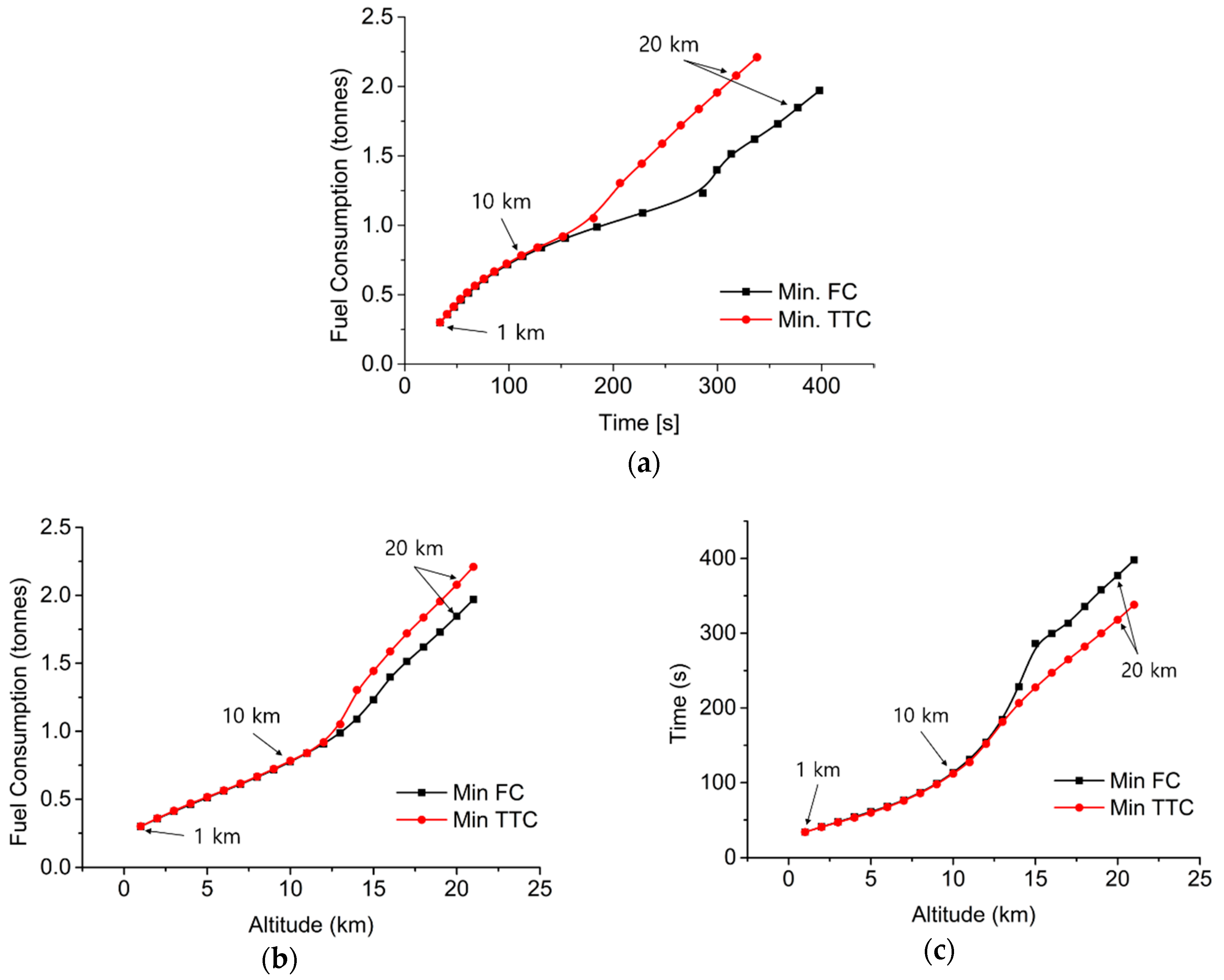
As mentioned in Section 2.6, the minimum FC and TTC solution paths were the bounds of Pareto fronts where trade-off optimal solutions lie within. The minimum FC results had almost equivalent values with the ones of minimum TTC that later diverged to take individual trajectories (Figure 3). One could even intuitively find that a diverging point of two solution trajectories occurred at around 10 to 12 km.

3.2. Terminal Residual Analysis (TRA) and Modified TRA

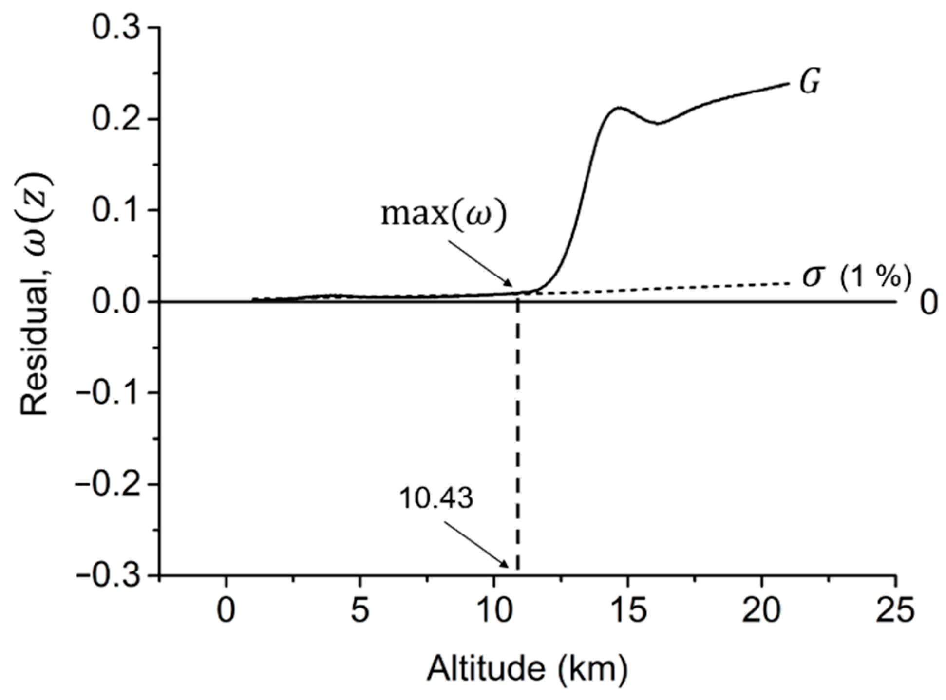
The residual between B-splined minimum FC and TTC solution data at $t_E$ was plotted with the criterion of $\sigma =1$ from the minimum FC solution in Figure 4, as proposed in Section 2.6. The altitude for Aircraft 1 was 10.43 km at max$\left(\omega \left(z\right)\right)$, at which the residual value started to deviate dramatically from the $\sigma$ range.

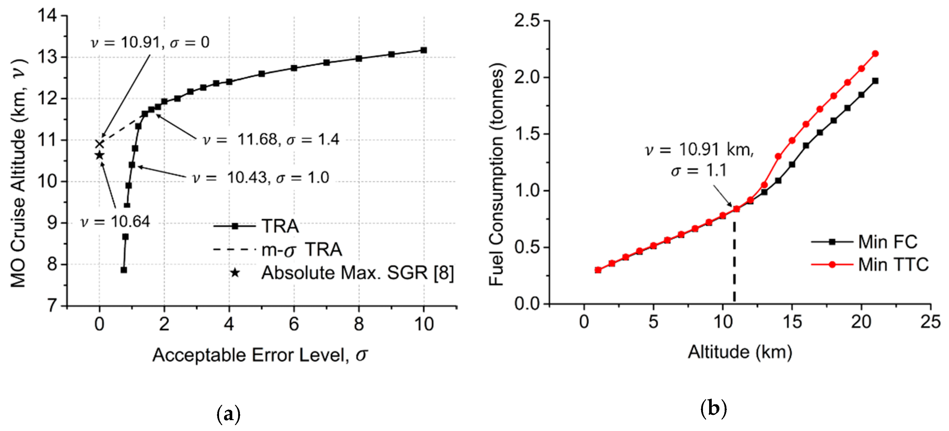
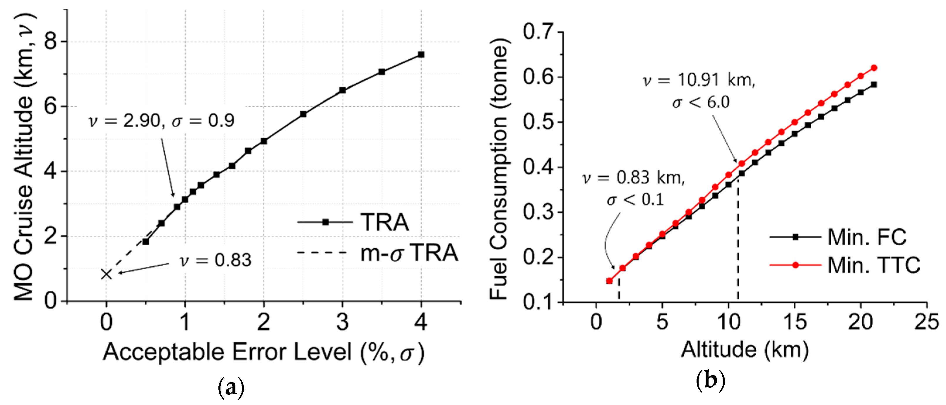
It was clear that the optimum cruise altitude would vary depending on the value of $\sigma$, and the effect of the variation of $\sigma$ was plotted in Figure 5a. Since $\nu$ fell dramatically after a certain level of $\sigma$, an extrapolated line was drawn from a point at which the first local maximum $\left(d^2\nu /d{\sigma }^2=0\right)$ counting from $\sigma =0$ was located at $\sigma =1.4$. The linearly extrapolated segment was named a marginally acceptable error level (m-$\sigma$). The MOCA value with original TRA approaching towards $\sigma =0$ fell dramatically after $\sigma =1.4$ but the one with m-$\sigma$ TRA gradually fell until $\sigma =0$, adapting the trends in the previous solution segments. The modified approach added a feasible tendency for the low-$\sigma$ region.

The m-$\sigma$ TRA at $\sigma =0$ resulted in the minimum fuel, optimum cruise altitude of 10.91 km. This value was close to the optimum cruise altitude of 10.64 km from the Ref. [9] for the absolute maximum specific ground range (SGR). The difference in the determined MOCA of the present study to the Ref. [9] was 2.5%. When the optimum cruise altitude MOCA of 10.91 km was considered, the corresponding $\sigma$ value for Aircraft 1 was close to 1.1 in Figure 5b. It meant that a transition in the flight mode from minimum FC to minimum TTC was possible at about 11 km, with just additional fuel usage of 1.1%. The details of this argument were further discussed in Section 4.3.

3.3. Optimized Climb Trajectory to Given Altitudes

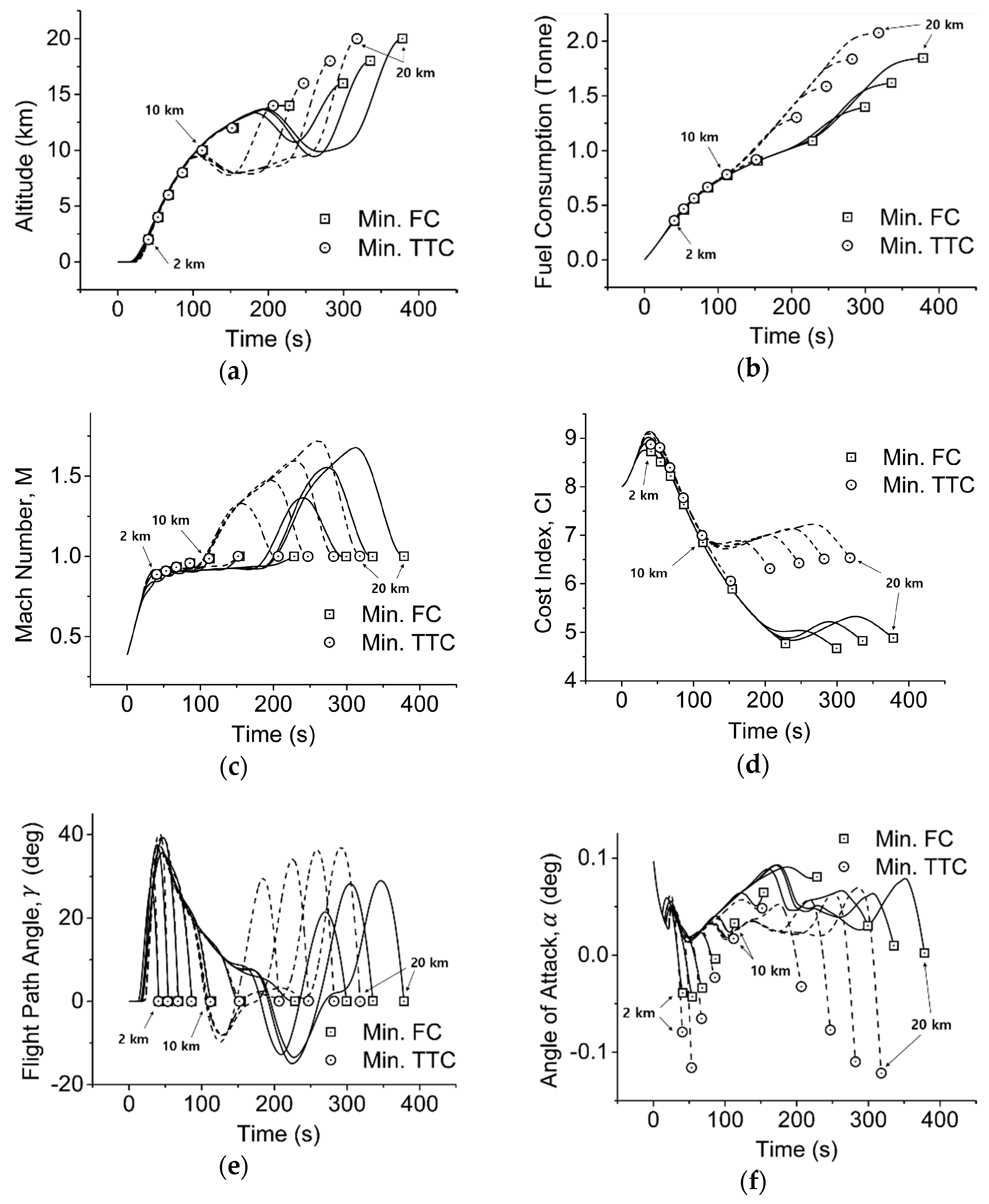
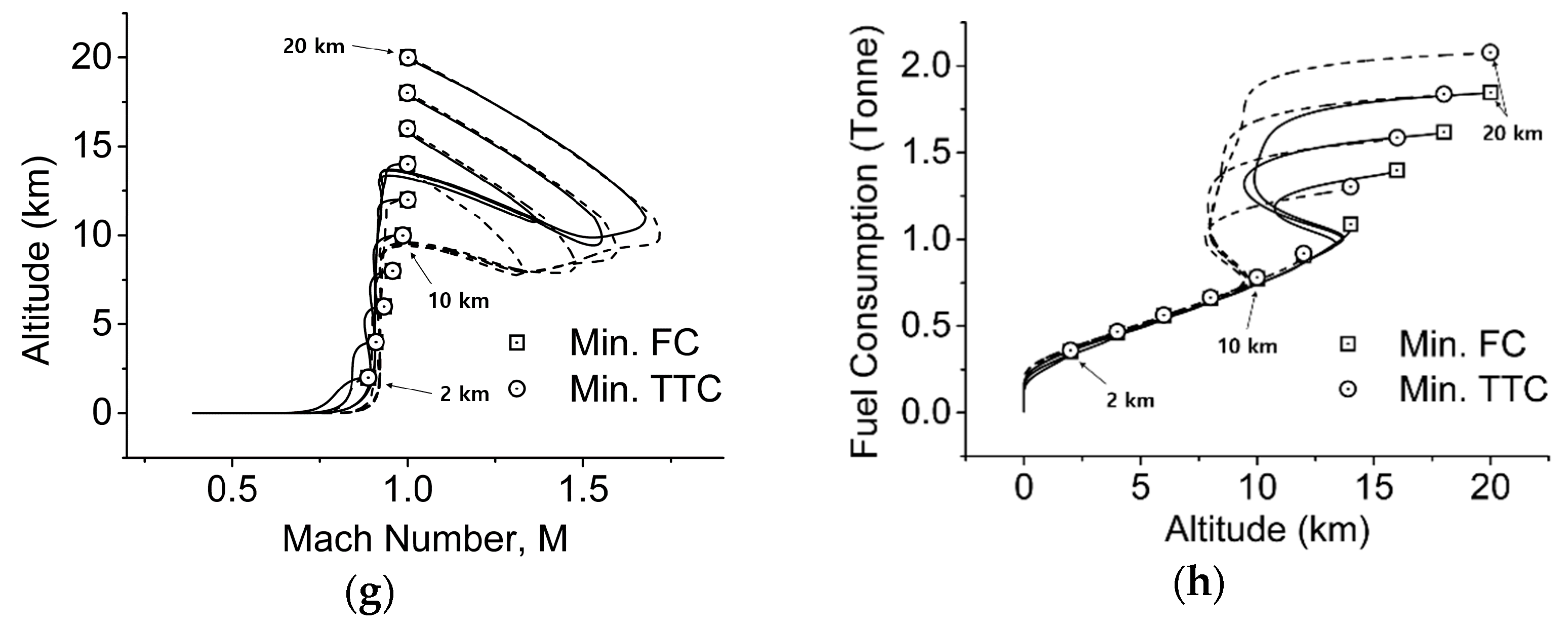
The climb trajectories of minimum FC and TTC were analyzed by plotting the individual trajectory curves by imposing equally spaced altitude values (Figure 6). The properties of altitude $z$, fuel consumption (FC), Mach number $M$, cost index ($\mathrm{CI}$), flight path angle $\gamma$, and angle of attack $\alpha$ were plotted. All results similar trends of diverging solutions curves from one another at a certain near-intersecting point and the dramatic differences between the trajectories after the bifurcation. One exception was $M$ in Figure 6g, where the final solution set was identical in both objectives. It may be because of fixed boundary conditions for the final speed of the aircraft ($V=295 \left[\mathrm{m}/\mathrm{s}\right])$ and the same target altitude. The equation for $M$ is $M=V/d$, where $d$ is the speed of sound, which was constant at the given elevations, hence making the calculated final $M$ in both objectives equivalent.

3.4. Optimized Trajectory to MOCA

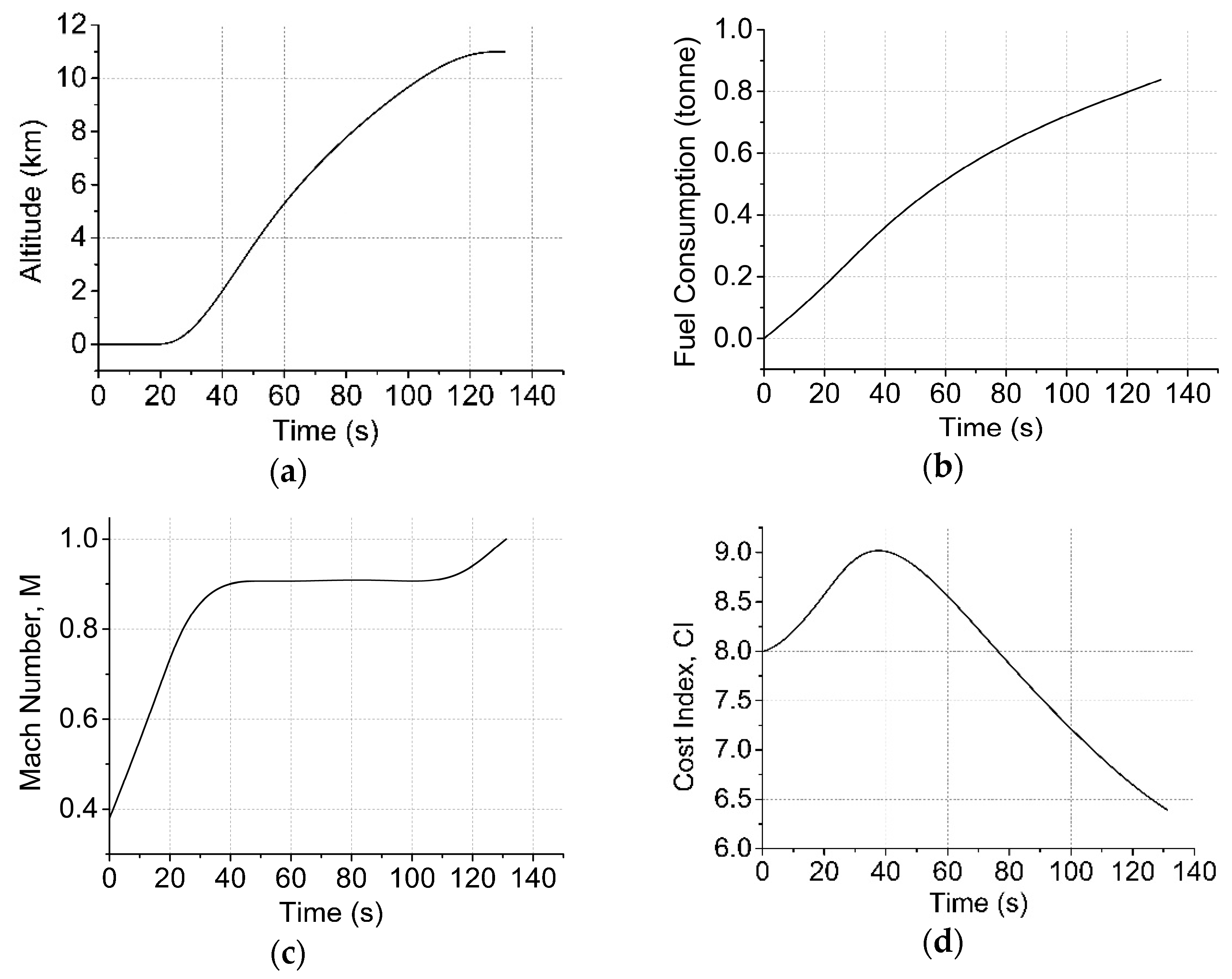
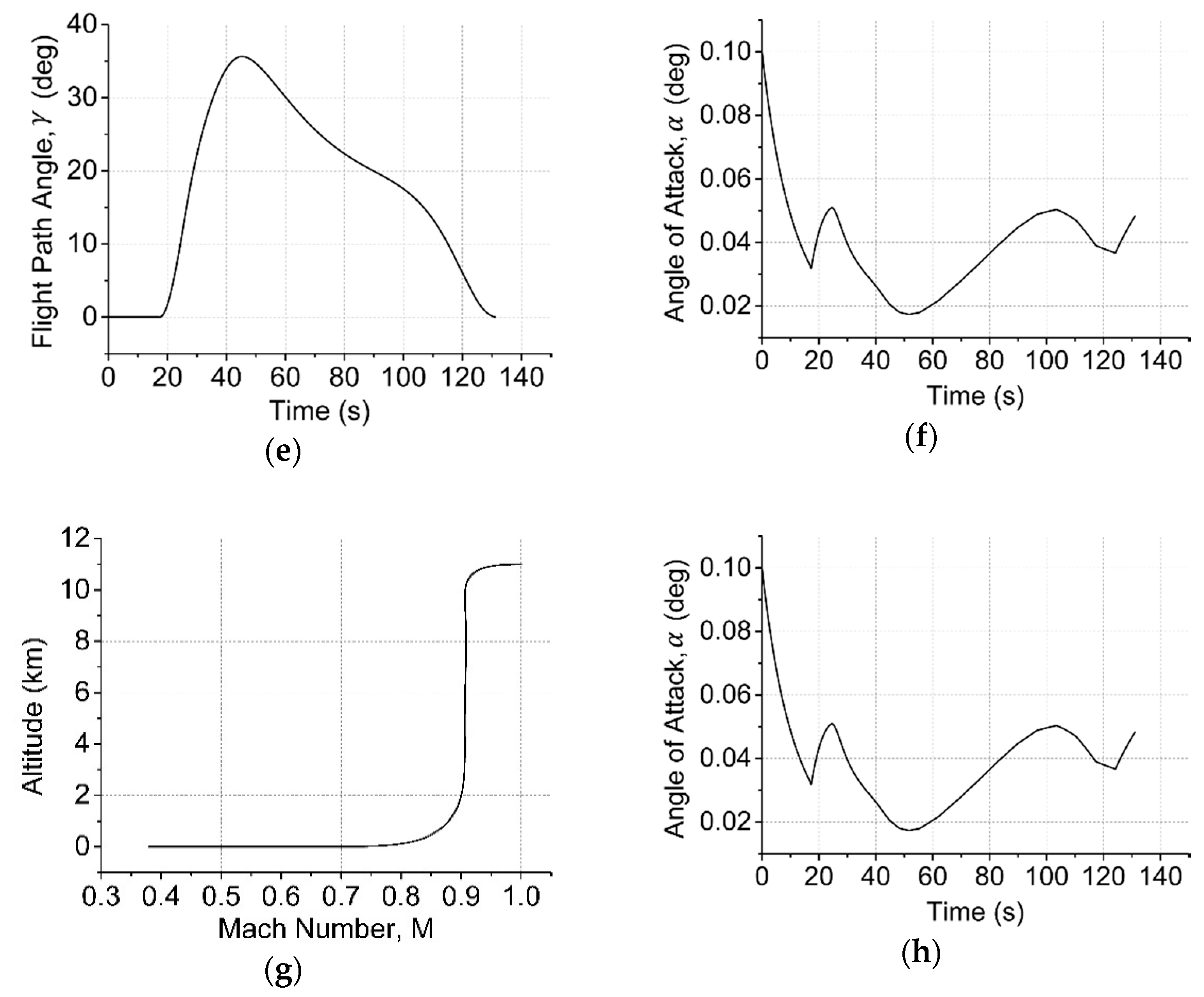
As shown in Figure 7, the altitude-specific, optimized trajectories at the minimum FC and TTC demonstrated similar patterns of overlapping line segments during the initial stage of the climb. Hence, the MOCA specific, minimum FC climb paths were plotted in Figure 7, where MOCA was approximated to be 11 km (which was 10.91 km). Similar to Figure 7, the properties of altitude $z$, fuel consumption (FC), Mach number $M$, cost index ($\mathrm{CI}$), flight path angle $\gamma$, and angle of attack $\alpha$ were plotted. Specifically, $z$ continuously increased until it reached the desired MOCA (Figure 7a), and FC showed an identical trend in Figure 7b,h. $M$ increased steeply until a value of 0.9 in Figure 7c, which then increased to 1.0 at the end of the trajectory. Figure 7g had a similarity with Figure 7c for having $M$ in relation. $\gamma$ and $\alpha$ varied continuously over the course of the trajectory in Figure 7e,f. $\mathrm{CI}$in Figure 7d also changed over time.

4. Discussion

4.1. Effectiveness of Terminal Residual Analysis (TRA) and Modified TRA

The minimum FC and TTC trajectory solutions were generated, and the values at $t_E$ were plotted to show the gradual increase in minimum FC and TTC to the given altitude (Figure 3a). The trends in the ascension were similar in both trajectories but diverged from a certain altitude (Figure 3 and Figure 6). Using the novel residual method proposed in this study, TRA, an acceptable error level $\sigma$ was selected to be 1, which acted like a terminal residual criterion (Figure 4). In this specific application on the determination of the multi-objective cruise altitude, the residuals abruptly increase from $\max \left(\omega \left(z\right)\right)$, which gave TRA-determined altitude, MOCA, satisfying the given multi-objectives. TRA initially failed to provide feasible solutions at lower $\sigma$ values, and a modified m-$\sigma$ TRA was proposed, which linearly extrapolated the optimized solution curve towards $\sigma =0$. It took account of only the points before the first local maximum of $d^2\nu /d{\sigma }^2$ near the turning point, where $\nu$ represents the MOCA. Substituting the fuel-saving cruise altitude value obtained from m-$\sigma$ TRA to the original TRA argument yielded the desired MOCA values denoting the required additional fuel usage from the minimum FC cruise altitude to achieve the minimum FC and TTC cruise altitude.

The extrapolated value from m-$\sigma$ TRA was 10.91 km at $\sigma =0$, and this value was almost equivalent to the cruise altitude of 10.64 km for absolute maximum specific ground range (SGR) from Ref. [9]. The authors believe that this was a very close estimation with computational simulation as the value from Ref. [9] was based on the accumulated, regressed statistical result of more than 200,000 actual flight data. Hence, TRA had proven its value in finding the optimum aircraft cruise altitude achieving minimum FC, which then could be implemented to acquire the minimum FC and TTC MOCA value with the supplemental method, m-$\sigma$ TRA.

The continuous climb path in the present results was similar to the fuel consumption model in Ref. [21]. Ref. [21] adopted a CCO model to optimize fuel consumption during the climb, which introduced external influences such as crosswind. The accuracy was 96%, and the maximum amount of fuel saved was 12%. The current study also had a continuous climb path with reliable atmospheric model and aircraft aerodynamic data showing a difference of 2.5% in the altitude solution. While the model in Ref. [21] considered various external factors such as crosswind, our study did not employ any external factors in the calculation. Hence, the present study is significant in two aspects: first, the proposed novel methods, TRA and m-σ TRA, were robust even without the consideration of external factors such as crosswind, and second, such external factors were not significant in the determination of the optimized performance of long-range flight. The latter, especially, would be valid as Ref. [9] already suggested that 46.8% of 200,000 flight data already had less than 1% benefit from the optimization.

Additionally, the MOCA value within $\sigma =2.0$ in the m-$\sigma$ TRA line, fell below 12 km (Figure 5a), leading to the MOCA range of 10.91 km to 11.97 km. The optimum cruise altitudes determined in the statistical results of Refs. [9,51] were 10.64, 11.19, 11.67, and 11.46 km, which implies that the altitude range calculated in the present study was appropriate.

4.2. Difference in TRA and Modified TRA

A newly proposed method, TRA, was modified into m-$\sigma$ TRA as the original TRA with $\sigma$ below a certain level changed abruptly. Such abrupt change indicated that $\sigma$ was critical in determining the multi-objective goal in this study. The residual value below the MOCA of 11.5 km was nearly constant, making a low $\sigma$ criterion below 1.4% ineffective. The linearly extrapolated value of minimum FC at $\sigma =0$ was validated with Ref. [9], as discussed in Section 4.1. Hence m-$\sigma$ could also be an alternative approach for such cases of significantly low $\sigma$.

4.3. Optimum Altitude MOCA with Minimum FC and TTC

The altitude determined with the m-$\sigma$ TRA method at $\sigma =0$ was the MOCA only with minimum FC objective. As described in Section 3.2, this approach incorporated with the TRA could be utilized to determine the MOCA. MOCA satisfied both the minimum FC and TTC at any altitude with the additional fuel usage denoted as $\sigma$. The initial selection of $\sigma =1$ was to find the cruise altitude showing the potential fuel reduction within 1%, which eventually was determined to be 10.43 km, and its difference to the altitude 11.68 km, selected on m-$\sigma$ TRA, seemed relatively large concerning only a difference of 0.4 in the value of $\sigma$. Interestingly, the difference in altitudes became minimum with increasing $\sigma$ (Figure 5). This result emphasized the difficulties in achieving both objectives simultaneously for an optimal altitude, which varies even with the slightest changes in $\sigma$.

Another interesting point here is that the minimum FC altitude, 10.91 km, was about 0.8 km lower than the MOCA at $\sigma =1.4$ (11.68 km). As mentioned in Section 1, a climb to a higher altitude takes advantage of lower air density for reduced aerodynamic drag but consequently consumes extra fuel for ascension. Hence, cruising at the MOCA at $\sigma =1.4$ may enjoy the minimum FC travel with considerably reduced travel time (TT) due to reduced aerodynamic drag, but the same at the MOCA at the adjusted $\sigma =1.1$ may enjoy the fuel-economy even with higher aerodynamic drag than the former. In detail, the MOCA with the minimum FC and TTC could be achieved at an altitude of 10.91 km with an additional fuel usage of 1.1% of the fuel used for minimum fuel climb to an altitude of 10.91 km. It implies the potential for flight mode transition between the single-objective, minimum FC, and the multi-objective, minimum FC and TTC. With this argument, an aircraft cruising at an altitude of 10.91 km could switch the flight mode from the minimum FC to the minimum FC and TTC with the extra fuel usage of 1.1%. Likewise, minimum FC and TTC cruise mode could be achieved at an altitude of 11.68 km with the additional fuel usage within 1.4% of the minimum FC cruise mode. The MOCA results of different s values provided quantitative explanations for the theory and the transition criterion for the flight mode between single-objective, the minimum FC, and the multi-objective, the minimum FC and TTC. Additionally, it also demonstrated that the fuel-economy may not always be achieved just by cruising at higher altitudes.

4.4. Individual Trajectory and Variable Cost Index (CI)

The trajectory solution at the determined MOCA of 10.91 km shows the trajectory of a supersonic jet (Figure 7). These graphs clearly show the relationships between the variables and parameters in this study, as described in Section 3.4. In the initial segment of the climb path, the aircraft accelerated by increasing $T$, which increased both $V$ and $M$ (Figure 7c). Throughout the whole trajectory, a fluctuated to make stable transitions in g, which resulted in a continuous and smooth climb path of the aircraft in terms of $z$ (Figure 7a), FC (Figure 7b,h), $M$ (Figure 7c), and $\mathrm{CI}$(Figure 7d).

Interestingly, $\mathrm{CI}$in (Figure 7d) varied over time. As mentioned in Section 1, numerous literatures targeting for multi-objective optimization of TOC usually employ a model with constant $\mathrm{CI}$ throughout a flight trajectory [4,6,8]. It may be due to the difficulties involved in the estimation of actual$\mathrm{CI}$ or an attempt to reduce the number of variables to solve in complex total cost equation such as:

$$C_{TOT}={{\displaystyle \int }}_0^{T_{flight}}fbr\left(t\right) dt+60·\mathrm{CI}·T_{flight},$$

(54)

where $C_{TOT}$ is the total cost, $\mathrm{CI}$ is the cost index as defined in this study, $T_{flight}$ is the cruise segment flight time, and $fbr\left(t\right)$ is the time-dependent aircraft fuel-burn rate function. This equation was re-written from Equation (6) of Ref. [52] by Dancila, B. D., et al. [8]. Given the number of variables involved, a range of constant $\mathrm{CI}$ values definitely would have made the problems more manageable. On the contrary, $\mathrm{CI}$ was not consistent throughout a flight path in this study (Figure 7d). Considering the realistic aspect of an actual flight path, the variation in $\mathrm{CI}$ during a flight is a more convincing phenomenon. This variation implies that the present approach was able to describe more pragmatic phenomena in aircraft motion.

4.5. Limitations

The first limitation is the use of aerodynamic data of a supersonic aircraft from Ref. [12] to find a multi-objective optimum cruise altitude. The selection of the optimum cruise altitude is a necessity in the economic management of airliners, and in most cases, the aircraft is subsonic. The use of a supersonic aircraft model may not be suitable to determine general cruise altitude, but as seen in Figure 7d, $M$ remains subsonic before reaching the cruise altitude. Such probably may have made the MOCA result in the present study similar to the statistically optimum cruise altitude of commercial airplanes. There also was lack of available data for subsonic aircraft in terms of thrust, Mach number and altitude. Such data was necessary for climb trajectory optimization. With the inadequacy in the available data, the authors tried to maintain the feasibility of the approach and obtained confident results for cruise altitude determination of a long-range flight. Overall, a more refined study could be conducted using the aerodynamic data of a subsonic aircraft.

The second limitation may be the applicability of the present methodology to determine the optimum cruise altitude for all-range flight. As mentioned in Section 1, Aircraft 1 and 2 are different in their specifications, especially in their initial weight and maximum thrust. This difference made the authors speculate Aircraft 1 to be the heavy, long-range plane for the former and lightweight, short-range plane for the latter. The results in Figure 8 clearly shows the difference where the present approach failed to achieve reasonable cruise altitude but only showed the potential to indicate the costs for the transition between two objectives. The present methodology may only apply to the cruise altitude determination of long-range flight, but since such flights require cruise altitude optimization the most [9], our approach could be a feasible solution for a cost-minimizing strategy.

This study proposed TRA and a modified TRA (m-$\sigma$ TRA) to determine an optimum cruise altitude satisfying minimum FC and TTC. Despite the promising results for long-range flight, further investigation would be necessary whether this approach is also suitable in other multi-objective optimization problems. The multi-objective optimization of aircraft trajectory problems may be the only problem solvable using the methods proposed in this study. Hence, this approach may need further validation in various optimization problems in future studies.

5. Conclusions

Multi-objective determination of cruise altitude of a supersonic aircraft was conducted using the Hermite-Simpson method. Individual optimum climb trajectories were generated in the discretized problem domain. A novel approach, TRA, was proposed with modified TRA, m-$\sigma$ TRA, to select the optimum cruise altitude with the minimum FC and TTC, where $\sigma$ also worked as a criterion to represent the magnitude of the transition between the single- or multi-objective flight mode. As a result, a multi-objective cruise altitude (MOCA) was determined to be 10.91 km for aircraft 1, which was validated with the statistical results of subsonic, commercial airliner data. The method presented in this study was found reliable in the multi-objective problem to determine the optimum cruise altitude of a long-range flight, achieving both minimum FC and TTC. Although various assumptions were used, this approach confirmed the complex multi-objective solution in aircraft cruise altitude problems in an environment formulated as realistic as possible. Further studies would be needed to verify this technique in other applications to validate its utility in other fields requiring multi-objective optimum solutions.

References

- IATA. Economic Performance of the Airline Industry: 2017 End-Year Report 2018. 2020. Available online: https://www.iata.org/en/iata-repository/publications/economic-reports/airline-industry-economic-performance-june-2020-report (accessed on 6 September 2020).
- Bureau of Transportation Statistics. First Quarter 2020 U.S. Airline Financial Data. 2020. Available online: https://www.bts.gov/newsroom/first-quarter-2020-us-airline-financial-data (accessed on 15 September 2020).
- Bureau of Transportation Statistics. U.S. Airlines Report Second Quarter 2020 Losses. 2020. Available online: https://www.bts.gov/newsroom/us-airlines-report-second-quarter-2020-losses (accessed on 15 September 2020).
- Dai, R.; Cochran, J.E. Three-Dimensional Trajectory Optimization in Constrained Airspace. J. Aircr. 2009, 46, 627–634. [Google Scholar] [CrossRef]
- Vavrina, M.; Howell, K. Multiobjective Optimization of Low-Thrust Trajectories Using a Genetic Algorithm Hybrid. In Proceedings of the AAS/AIAA Space Flight Mechanics Meeting, Pittsburgh, PA, USA, 9–13 August 2009. [Google Scholar]
- Franco, A.; Rivas, D. Minimum-Cost Cruise at Constant Altitude of Commercial Aircraft Including Wind Effects. J. Guid. Control Dyn. 2011, 34, 1253–1260. [Google Scholar] [CrossRef]
- Lovegren, J.; Hansman, R.J. Estimation of Potential Aircraft Fuel Burn Reduction in Cruise via Speed and Altitude Optimization Strategies; MIT International Center for Air Transport (ICAT): Cambridge, MA, USA, 2011. [Google Scholar]
- Dancila, B.; Botez, R.; Labour, D. Altitude Optimization Algorithm for Cruise, Constant Speed and Level Flight Segments. In Proceedings of the AIAA Guidance, Navigation, and Control Conference, Minneapolis, MI, USA, 13–16 August 2012. [Google Scholar]
- Jensen, L.; Hansman, R.J.; Venuti, J.C.; Reynolds, T. Commercial airline altitude optimization strategies for reduced cruise fuel consumption. In Proceedings of the 14th AIAA Aviation Technology, Integration, and Operations Conference, Atlanta, GA, USA, 16–20 June 2014. [Google Scholar]
- Antonakis, A.; Nikolaidis, T.; Pilidis, P. Multi-Objective Climb Path Optimization for Aircraft/Engine Integration Using Particle Swarm Optimization. Appl. Sci. 2017, 7, 469. [Google Scholar] [CrossRef] [Green Version]
- Rutowski, E.S. Energy approach to the general aircraft performance problem. J. Aeronaut. Sci. 1954, 21, 187–195. [Google Scholar] [CrossRef]
- Bryson, A.E., Jr.; Desai, M.N.; Hoffman, W. Energy-state approximation in performance optimization of supersonicaircraft. J. Aircr. 1969, 6, 481–488. [Google Scholar]
- Ong, S.Y. A model comparison of a supersonic aircraft minimum time-to-climb problem. In Proceedings of the 25th AIAA Aerospace Sciences Meeting, Reno, NV, USA, 12–15 January 1986. [Google Scholar]
- Pierson, B.L.; Ong, S.Y. Minimum-Fuel Aircraft Transition Trajectories. Math. Comput. Model. 1989, 12, 925–934. [Google Scholar] [CrossRef]
- Morimoto, H.; Chuang, J. Minimum-fuel trajectory along entire flight profile for a hypersonic vehicle with constraint. In Proceedings of the Guidance, Navigation, and Control Conference and Exhibit, Boston, MA, USA, 10–12 August 1998. [Google Scholar]
- Benson, D. A Gauss Pseudospectral Transcription for Optimal Control; Massachusetts Institute of Technology: Cambridge, MA, USA, 2005. [Google Scholar]
- Von Stryk, O.; Bulirsch, R. Direct and Indirect Methods for Trajectory Optimization. Ann. Oper. Res. 1992, 37, 357–373. [Google Scholar] [CrossRef]
- Hargraves, C.R.; Paris, S.W. Direct Trajectory Optimization Using Nonlinear-Programming and Collocation. J. Guid. Control Dyn. 1987, 10, 338–342. [Google Scholar] [CrossRef]
- Bayen, A.M.; Mitchell, I.M.; Oishi, M.M.K.; Tomlin, C.J. Aircraft autolander safety analysis through optimal control-based reach set computation. J. Guid. Control Dyn. 2007, 30, 68–77. [Google Scholar] [CrossRef]
- Tsiotras, P.; Bakolas, E.; Zhao, Y. Initial guess generation for aircraft landing trajectory optimization. In Proceedings of the AIAA Guidance, Navigation, and Control Conference, Portland, OR, USA, 8–11 August 2011. [Google Scholar]
- Roach, K.; Robinson, J. A terminal area analysis of continuous ascent departure fuel use at Dallas/Fort Worth international airport. In Proceedings of the 10th AIAA Aviation Technology, Integration, and Operations (ATIO) Conference, Fort Worth, TX, USA, 13–15 September 2010. [Google Scholar]
- Zhang, M.; Huang, Q.; Liu, S.; Zhang, Y. Fuel Consumption Model of the Climbing Phase of Departure Aircraft Based on Flight Data Analysis. Sustainability 2019, 11, 4362. [Google Scholar] [CrossRef] [Green Version]
- Pargett, D.M.; Ardema, M.D. Flight path optimization at constant altitude. J. Guid. Control Dyn. 2007, 30, 1197–1201. [Google Scholar] [CrossRef]
- NOAA; NASA; USAF. US Standard Atmosphere, 1976; National Oceanic and Atmospheric Administration: Washington, DC, USA, 1976; Volume 76.
- Herman, A.L.; Conway, A.C. Direct optimization using collocation based on high-order Gauss-Lobatto quadrature rules. J. Guid. Control Dyn. 1996, 19, 592–599. [Google Scholar] [CrossRef]
- Bryson, A.E.; Denham, W.F. A steepest-ascent method for solving optimum programming problems. J. Appl. Mech. 1962, 29, 247. [Google Scholar] [CrossRef]
- Gelfand, I.M.; Silverman, R.A. Calculus of Variations; Dover Publications: Mineola, NY, USA, 2000. [Google Scholar]
- Wan, F. Introduction to the Calculus of Variations and Its Applications; Routledge: London, UK, 2017. [Google Scholar]
- Leitmann, G. The Calculus of Variations and Optimal Control: An Introduction; Springer Science & Business Media: New York, NY, USA, 2013; Volume 24. [Google Scholar]
- Pontryagin, L.S. Mathematical Theory of Optimal Processes; Routledge: New York, NY, USA, 2018. [Google Scholar]
- Bryson, A.E. Applied Optimal Control: Optimization, Estimation and Control; CRC Press: Boca Raton, FL, USA, 1975. [Google Scholar]
- Thompson, G.L. Optimal Control Theory: Applications to Management Science and Economics; Springer: New York, NY, USA, 2006. [Google Scholar]
- Topputo, F.; Zhang, C. Survey of direct transcription for low-thrust space trajectory optimization with applications. In Abstract and Applied Analysis; Hindawi: London, UK, 2014. [Google Scholar]
- Nie, Y.; Faqir, O.; Kerrigan, E.C. ICLOCS2: Try this optimal control problem solver before you try the rest. In Proceedings of the 2018 UKACC 12th International Conference on Control (CONTROL), Sheffield, UK, 5–7 September 2018. [Google Scholar]
- Wachter, A.; Biegler, L.T. On the implementation of an interior-point filter line-search algorithm for large-scale nonlinear programming. Math. Program. 2006, 106, 25–57. [Google Scholar] [CrossRef]
- Barnes, W.; McCormick, W. Aerodynamics Aeronautics and Flight Mechanics; Wiley: New York, NY, USA, 1995. [Google Scholar]
- Daniel, D.; Livescu, D.; Ryu, J. Reaction analogy based forcing for incompressible scalar turbulence. Phys. Rev. Fluids 2018, 3, 094602. [Google Scholar] [CrossRef]
- Ryu, J.; Livescu, D. Turbulence structure behind the shock in canonical shock–vortical turbulence interaction. J. Fluid Mech. 2014, 756. [Google Scholar] [CrossRef] [Green Version]
- Ryu, J.; Lele, S.K.; Viswanathan, K. Study of supersonic wave components in high-speed turbulent jets using an LES database. J. Sound Vib. 2014, 333, 6900–6923. [Google Scholar] [CrossRef]
- Denham, W.F. Steepest-Ascent Solution of Optimal Programming Problems; Harvard University: Cambridge, MA, USA, 1963. [Google Scholar]
- Patterson, M.A.; Rao, A.V. GPOPS-II: A MATLAB software for solving multiple-phase optimal control problems using hp-adaptive Gaussian quadrature collocation methods and sparse nonlinear programming. ACM Trans. Math. Softw. (TOMS) 2014, 41, 1–37. [Google Scholar] [CrossRef] [Green Version]
- Prautzsch, H.; Boehm, W.; Paluszny, M. Bézier and B-Spline Techniques; Springer Science & Business Media: New York, NY, USA, 2002. [Google Scholar]
- Pareto, V. Manual of Political Economy: A Critical and Variorum Edition; OUP Oxford: New York, NY, USA, 2014. [Google Scholar]
- Deb, K. Multi-Objective Optimization Using Evolutionary Algorithms; John Wiley & Sons: Chichester, UK, 2001; Volume 16. [Google Scholar]
- Zadeh, L. Optimality and non-scalar-valued performance criteria. IEEE Trans. Autom. Control 1963, 8, 59–60. [Google Scholar] [CrossRef]
- Bureau of Transportation Statistics. 2016 Annual and 4th Quarter Airline Finalcial Data. Available online: https://www.bts.gov/newsroom/2016-annual-and-4th-quarter-airline-financial-data (accessed on 12 September 2020).
- Bureau of Transportation Statistics. 2017 Annual and 4th Quarter U.S. Airline Financial Data. Available online: https://www.bts.gov/newsroom/2017-annual-and-4th-quarter-us-airline-financial-data (accessed on 12 September 2020).
- Bureau of Transportation Statistics. 2018 Annual and 4th Quarter U.S. Airline Financial Data. Available online: https://www.bts.gov/newsroom/2018-annual-and-4th-quarter-us-airline-financial-data (accessed on 12 September 2020).
- Bureau of Transportation Statistics. 2019 Annual and 4th Quarter U.S. Airline Financial Data. Available online: https://www.bts.gov/newsroom/2019-annual-and-4th-quarter-us-airline-financial-data (accessed on 12 September 2020).
- Roberson, B. Fuel Conservation Strategies: Cost index explained. AERO 2007, 2, 26–28. [Google Scholar]
- Jensen, L.; Hansman, R.J.; Venuti, J.; Reynolds, T. Commercial airline speed optimization strategies for reduced cruise fuel consumption. In Proceedings of the 2013 Aviation Technology, Integration, and Operations Conference, Los Angeles, CA, USA, 12–14 August 2013. [Google Scholar]
- Liden, S. Optimum cruise profiles in the presence of winds. In Proceedings of the IEEE/AIAA 11th Digital Avionics Systems Conference, Seattle, WA, USA, 5–8 October 1992. [Google Scholar]
Figure 1.
The main concept of Hermite collocation methods (reproduced from Figure 1, Ref. [33]). This method captures the local derivatives of the state variables to minimize the error between state derivatives from dynamics and polynomial differentiation.
Figure 2.
Longitudinal dynamics of an aircraft represented in point-mass approximation.
Figure 3.
The minimum FC and TTC solutions at in an altitude interval of 1 km. The plots of (a), TTC against FC; (b) altitude against FC; (c) altitude against TTC are illustrated.
Figure 4.
The plot of residuals between the minimum TTC and FC solution data which graphically illustrated the concept of the selection criterion described in the Section 2.6. , residual between minimum FC and TTC solution; , acceptable error level (AEL); , terminal residual.
Figure 5.
The effect of different σ on the MOCA (a) and the corresponding MOCA for the minimum TTC objective (b) of Aircraft 1. (a) The AEL and the m-σ TRA line segment were plotted against the MOCA, and along the TRA line, respectively. The optimum cruise altitude to achieve absolute specific ground range (SGR) from Ref. [9] was illustrated as a star (black). The m- TRA value and the absolute maximum SGR value from the reference have an almost identical fuel-saving optimum cruise altitude. (b) The altitude 10.91 was the predicted minimum FC cruise altitude with m-σ TRA. The corresponding altitude along the minimum TTC trajectory is achieved with σ = 1.1. AEL, acceptable error level, σ; MOCA, multi-objective cruise altitude; TRA, terminal residual analysis; SGR, specific ground range.
Figure 6.
Climb path trajectories of: altitude , fuel consumption (FC), Mach Number , cost index (), flight path angle , angle of attack in terms of time , , and for Aircraft 1 at the altitudes of interval of 2 km from 2 to 20 km. (a) Time against ; (b) time against FC; (c) time against ; (d) time against ; (e) time against ; (f) time against ; (g) against ; (h) against FC.
Figure 7.
Climb path trajectories of: altitude , fuel consumption (FC), Mach Number , cost index (), flight path angle , angle of attack in terms of time , , and for Aircraft 1 at the multi-objective cruise altitude (MOCA) of 11 km. (a) Time against ; (b) time against FC; (c) time against ; (d) time against ; (e) time against ; (f) time against ; (g) against ; (h) against FC.
Figure 8.
The effect of different σ on the MOCA (a) and the corresponding MOCA for the minimum TTC objective (b) of Aircraft 2. (a) The AEL and the m-σ TRA line segment were plotted against the MOCA, and along the TRA line, respectively. The AEL, , is plotted against multi-objective cruise altitude (MOCA) , and linearly extrapolated m- TRA is also drawn along the terminal residual analysis (TRA) line. (b) The altitude 10.91 km was the predicted minimum FC cruise altitude with m-σ TRA of Aircraft 1, and the corresponding altitude along the minimum TTC trajectory in Aircraft 2 is achieved with . AEL, acceptable error level, σ; MOCA, multi-objective cruise altitude; TRA, terminal residual analysis.