Statistical Arbitrage in Emerging Markets: A Global Test of Efficiency
by
 , , and
Karen Balladares
1 ,
,
José Pedro Ramos-Requena
2,
Juan Evangelista Trinidad-Segovia
2,* and
and
Miguel Angel Sánchez-Granero
3
1
Facultad de Ciencias Administrativas, Universidad de Guayaquil, 090514 Guayaquil, Ecuador
2
Departamento de Economía y Empresa, Universidad de Almería, Carretera Sacramento s/n, La Cañada de San Urbano, 04120 Almería, Spain
3
Departamento de Matemáticas, Universidad de Almería, Carretera Sacramento s/n, La Cañada de San Urbano, 04120 Almería, Spain
*
Author to whom correspondence should be addressed.
Mathematics 2021, 9(2), 179; https://0-doi-org.brum.beds.ac.uk/10.3390/math9020179
Submission received: 7 December 2020
/
Revised: 11 January 2021
/
Accepted: 15 January 2021
/
Published: 18 January 2021
(This article belongs to the Special Issue Mathematics and Mathematical Physics Applied to Financial Markets)
Abstract
:In this paper, we use a statistical arbitrage method in different developed and emerging countries to show that the profitability of the strategy is based on the degree of market efficiency. We will show that our strategy is more profitable in emerging ones and in periods with greater uncertainty. Our method consists of a Pairs Trading strategy based on the concept of mean reversion by selecting pair series that have the lower Hurst exponent. We also show that the pair selection with the lowest Hurst exponent has sense, and the lower the Hurst exponent of the pair series, the better the profitability that is obtained. The sample is composed by the 50 largest capitalized companies of 39 countries, and the performance of the strategy is analyzed during the period from 1 January 2000 to 10 April 2020. For a deeper analysis, this period is divided into three different subperiods and different portfolios are also considered.
1. Introduction
The Efficient Market Hypothesis (EMH) was introduced by Cootner [1] and Samuelson [2]. Recently, Fama [3] developed three states of efficiency:
- Strong form efficiency states all information in a market, whether public or private, is contained in the stock price.
- Semi-strong efficiency means that all public information is calculated into a stock’s current share price.
- Weak form efficiency implies that all past prices of a stock are reflected in today’s stock price.
When markets are fully efficient, neither technical analysis, fundamental analysis nor insider information enable an investor to obtain returns greater than those that could be obtained by holding random portfolios or individual stocks with the same risk.
Today, many financial economists and investors accept that the presence of the first two scenarios are almost impossible even in high capitalized markets (Campbell et al. [4] and Grossman and Stiglitz [5]); this is why the weak-form version of market efficiency is the most tested criterion in the financial literature. To test the level of market efficiency has been a quite popular topic in financial literature because, if a market is not efficient, this means that future stock prices are somewhat predictable based on past stock price which enable investors to earn excess risk adjusted rates of return.
One of the most interesting works is the one by Markiel and Fama [6], where authors considered that the weak and the semi strong forms of efficiency were strongly supported by their results. After this work, some researchers have tested whether technical analysis is able to provide abnormal returns to the investors (see, for example, Fama and Blume [7], Fama and French [8], Olson [9], Rosillo et al. [10], Shynkevich [11], Metghalchi et al. [12] or Bobo and Dinica [13]).
Other researchers decided to analyze price adjustments after market events (see, for example, Pettit [14], Asquith and Mullins [15] and Michaely, Thaler and Womack [16], Aharony and Swary [17] and Kalay and Loewenstein [18], among others).
Another part of the financial literature has tested the EMH based on the statistical implication of this hypothesis: that stock returns follow a random walk. Interesting contributions are Lo and MacKinlay [19], Lima and Tabak [20], Fifield and Jetty [21], Charles and Darné [22], Al-Ajmi and Kim [23] or Mlambo and Biekpe [24] between others.
Recent contributions have come from some mathematicians and physicians that have focused their attention on Mandelbrot’s critics to the EMH [25]. Mandelbrot proposed that stock prices follow a fractional Brownian motion and not a random walk. One of the implications of this assumption is that stock prices exhibit long memory, which is against the EMH. On this basis, to explore the presence of market memory is an alternative method to test the market efficiency. Relevant contributions are Beben and Orłowski [26], DiMatteo et al. [27], Zunino et al. [28], Cajueiro [29], Kristoufek [30], Ferreira et al. [31], Kristoufek [32] and Dimitrova et al. [33].
This paper goes along a similar line, and it is based on the recent novel approach introduced by Sanchez et al. [34], where the authors analyzed the relationship between market efficiency and a statistical arbitrage technique based on Hurst exponent [35]. We propose to extend the analysis to the 50 largest capitalized companies in 39 so-called advanced and emerging countries to see if a Pairs Trading strategy based on Hurst Exponent, which is a market memory indicator, can obtain a significant profit during different periods.
Our results will show that emerging markets are not efficient while the developed ones are, for most of the period, under study. We will prove that the method used is robust by studying the return of the trades with each pair, considering the estimated Hurst exponent of the pair selection. We will show that, as expected, the lower the Hurst exponent of the pair series, the higher the return of the pair in the Pairs Trading strategy. The paper is structured as follows: Section 2 introduces the Pairs Trading technique based on Hurst exponent. In this section, we present the fundamentals of the Pairs Trading technique as well as the main contributions done by the financial literature. This section also introduces some relevant questions about Hurst Exponent and the Pairs Trading strategy. Section 3 contains the results of the different strategies developed. Finally, Section 4 presents the conclusions.
2. A Pairs Trading Technique Based on Hurst Exponent
2.1. Fundamentals of Pairs Trading
The strategy of statistical arbitrage arose in the 1980s. Since its birth, there have been different studies in this area.
The pioneer in investigating this strategy was Gatev et al. [36] who found statistically significant results using US market values during the period 1962–1997. Gatev et al. [37] carried out the study again extending the period until 2002 and obtaining average annualized higher returns of up to 11%. The authors concluded that these higher returns from this strategy are due to a reward for the application of the Law of One Price.
Elliott et al. [38] used a Gaussian Markov chain model to measure dispersion, while Do et al. [39] employed theoretical pricing methods. The cointegration approach was used by Vidyamurthy [40], Burgess [41], and Haque and Haque [42].
Perlin [43] used a Pairs Trading strategy in the Brazilian market, concluding that it works significantly, pointing out that positive superior returns are significant.
Do and Faff ([44,45]) used the distance method introduced by Gatev et al. during the period 2000–2009 and concluded that the Pairs Trading strategy was still profitable, but the profitability decreases over the time. This decline was attributed to a worsening of arbitrage risks and an increase in market efficiency. This is the first contribution where transaction costs are considered, showing that, from 2002 onwards, it generated losses.
Bowen et al. [46] developed their study taking intraday values and concluded that this strategy may be affected by transaction costs and speed of execution. They showed that the highest profitability is achieved at the first and last minute. Similar results are obtained by Liu et al. [47], where authors introduced an intraday trading strategy based on a conditional modeling to model spreads between pairs of stocks. The authors found remarkable returns including transaction costs during specific periods.
Huck [48] introduced a forecasting methodology using a combination of Neural Networks techniques and multi-criteria decision-making methods; Xie and Wu [49] proposed an alternative approach using the copula technique that is able to capture the structure of dependence of co-movement between two assets. Göncü and Akyildirim [50] supported the strategy of statistical arbitrage by assuming that the dispersion of two assets follows an Ornstein–Uhlenbeck process around a long-term equilibrium level.
Avellaneda et al. [51] studied the strategy of statistical arbitrage employing US actions. To do this, they used Principal Component Analysis and sectorial ETFs. In both cases, they detected opposite trading signals, considering the waste the returns of the shares and modeling the investment process.
Krauss [52] examined the literature on pairs trading strategy. It did so by dividing it into five groups; firstly, it studied the distance method; secondly, it used the co-integration method, it used the stochastic approach to identify the optimal portfolio trends, and, finally, it selected other approaches with some limitations in the literature.
Rad et al. [53] studied the performance of Pairs Trading based on the distance, cointegration, and copula methods on the entire US equity market from 1962 to 2014 including trading costs. The authors found that all strategies show positive results and mainly during periods of significant volatility.
Ramos-Requena et al. [35] introduced the Hurst exponent as a selection method in Pairs Trading. The authors found that this new methodology gives better results than the classical methodologies such as the distance or the correlation method. In a recent contribution [54], these authors proposed an alternative method to correlation and cointegration called the HP method.
Finally, all of these contributions are focused on the methodology for pairs selection. In a different line, Ramos-Requena et al. [55] introduced different models to calculate the amount of money that must be allocated to each stock. The authors showed these new alternatives perform better than the usual Equal Weight method.
2.2. Notes on Hurst Exponent
The hypothesis that price variations are well-described by means of a fractional Brownian motion was introduced by Mandelbrot [25]. This process is a long memory generalization of the Brownian motion process with a self-similarity exponent (called Hurst exponent) different to 0.5. Thus, when the process is a Brownian motion, the Hurst exponent (H) is equal to 0.5; when it is persistent, H will be greater than 0.5, and, finally, when it is anti-persistent, then H will be less than 0.5.
The Hurst exponent was introduced by Hurst in 1951 [56] to deal with the problem of reservoir control near the Nile River Dam, but, in recent decades, its application has been widely extended in economics in general and in finance in particular (see López-García and Ramos-Requena [57] for a literature and methodological review). There is also some novel applications, like Trinidad-Segovia et al. [58] and Nikolova et al. [59], where it was used to study volatility clusters.
Ramos-Requena et al. [35] used the Hurst exponent as a management tool for statistical arbitrage strategies based on the concept of reversion to the mean.
Since the first method introduced by Hurst [56], the R/S analysis, different methodologies have been proposed. In this paper, we use the Generalized Hurst exponent () introduced by Barabasi and Vicsek [60].
This algorithm is calculated as follows:
where X is the series (in this paper, X will be the pair series as defined in Section 2.3), can vary between 1, and , is usually chosen as a quarter of the length of the series, and denotes the sample average over the time window.
Therefore, the GHE is defined on the basis of the behavior on the scale of the statistic given in (1), given by the power law:
where is the Hurst exponent, which characterizes the power law scaling.
2.3. Methodology
Our trading methodology is developed as follows:
Firstly, we normalize the stock prices. If we consider shares A and B, and their share prices are and , respectively, the pair series is defined as:
where b is a constant, and it is used to normalize the stock prices.
To calculate the value of b, we will use the method described by Ramos-Requena et al. [55], called minimizing distance.
The function will be minimized, looking for the value of b, such that and have the minimal distance, where and .
Now, the pairs will be selected, using the Hurst exponent approach as developed in Section 2.2. Here, we look for pairs such that the Hurst exponent of their pair series is as low as possible.
Finally, the trading strategy will be developed. If s is the pair series, m the average of the series s, and the standard deviation of [62], then:
- If , the pair will be sold at . The position will be closed when or .
- If , the pair will be bought at . The position will be closed when or .
3. Experimental Results
This section shows the main results obtained by applying the Pairs Trading strategy. This will be done by taking the 50 largest capitalized companies in 39 countries. Three sub-periods (From 1 January 2000 to 31 December 2007, the second period is from 1 January 2007 to 31 December 2014 and the last period is from 1 January 2014 to 10 April 2020) and different portfolios (of 30, 40, and 50 pairs) are also considered. In this study, we considered transaction costs of 0.01%. Table A1 includes the classification of the countries studied between emerging and advanced.
Table A2, Table A3 and Table A4 show the results obtained for the period 2000–2007 for the portfolios composed of 30, 40, and 50 pairs. It can be seen that the highest profits after transaction costs are obtained for emerging countries, especially in South Africa (71.21%, 65.84%, and 65.68%), Japan (32.61%, 28.99%, and 28.87%) and Israel (28.99%, 23.54%, 25.76%). Japan is not an emerging country, but the long-lasting negative bias in its stock market has caused many investors to forget about it. Regarding Israel, the country cannot be considered an emerging country, but its stock market posseses a very low capitalization, even below emerging countries such as South Africa or Indonesia. For the same period, developed markets, especially the United States, show significantly negative returns after transaction costs (−12.87%, −11.61%, and −10.05%) as well as other European countries such as Norway, Russia, and Portugal.
If we look at the Sharpe ratio values, we can see that a value above 1 is obtained for countries such as South Africa (1.98, 1.6 and 1.45), Lebanon (1.11), Namibia (1.1), Israel, and Japan. Against these values, we find Norway with a negative Sharpe ratio (−0.74), and the United States (−0.35, −0.31, and −0.26).
Table A5, Table A6 and Table A7 show results obtained for the period 2007–2014. During this period, we are faced with the subprime crisis, which led to a large drop in the values of the main world stock market indexes as a consequence of the volatility increase. Despite this, it can be seen that the greatest benefits are obtained for emerging countries such as Israel (54.25%, 51.59% and 47.32%) and South Africa (33.80%, 32.73% and 29.88%). In this ranking, we find some European countries with significant benefits, such as Portugal (36.82%, 24.75% and 10.91%), Netherlands (26.26%, 31.27% and 27.94%), and Greece (19.85%, 19.88% and 19.89%). It is not like in the previous period, when it is clear that the developed countries are at a disadvantage in this strategy; for example, the United States is making positive gains in this period (1.30%, 4.13%, and 4.66%). The positive results could be attributed to the high volatility and correlation during financial crisis. These results are congruent with previous finding of Ramos Requena et al. [35] and Lopez García et al. [63].
The Sharpe ratio will indicate that the best investment options will be in countries such as Lebanon (2.53), Israel (1.44, 1.35, and 1.23), and South Africa (1.31, 1.28, and 1.08).
Finally, Table A8, Table A9 and Table A10 present the main results obtained for the period 2014–2020 for the portfolios composed of 30, 40, and 50 pairs. In this period, the highest profitability after transaction costs is for Greece (59.71%, 47.70%, 42.39%). Two other emerging countries (Colombia and South Africa) are among the most profitable to apply the Pairs Trading strategy during this period. France, Spain, or Dubai are the least profitable to invest in, with negative returns during this period.
If we look at the risk, the values of the Sharpe ratio indicate that Lebanon (3.85) and Colombia (2.11, 1.9 and 1.84) are the most appropriate countries. However, according to this ratio, it is not advisable to invest in countries such as Mexico or Dubai with a negative Sharpe ratio value.
One of the main features of Pairs Trading’s strategy is its market neutrality. As presented by Ramos-Requena et al. [35], to comply with this property, investors must consider pairs with a value of the Hurst exponent (H) below 0.5.
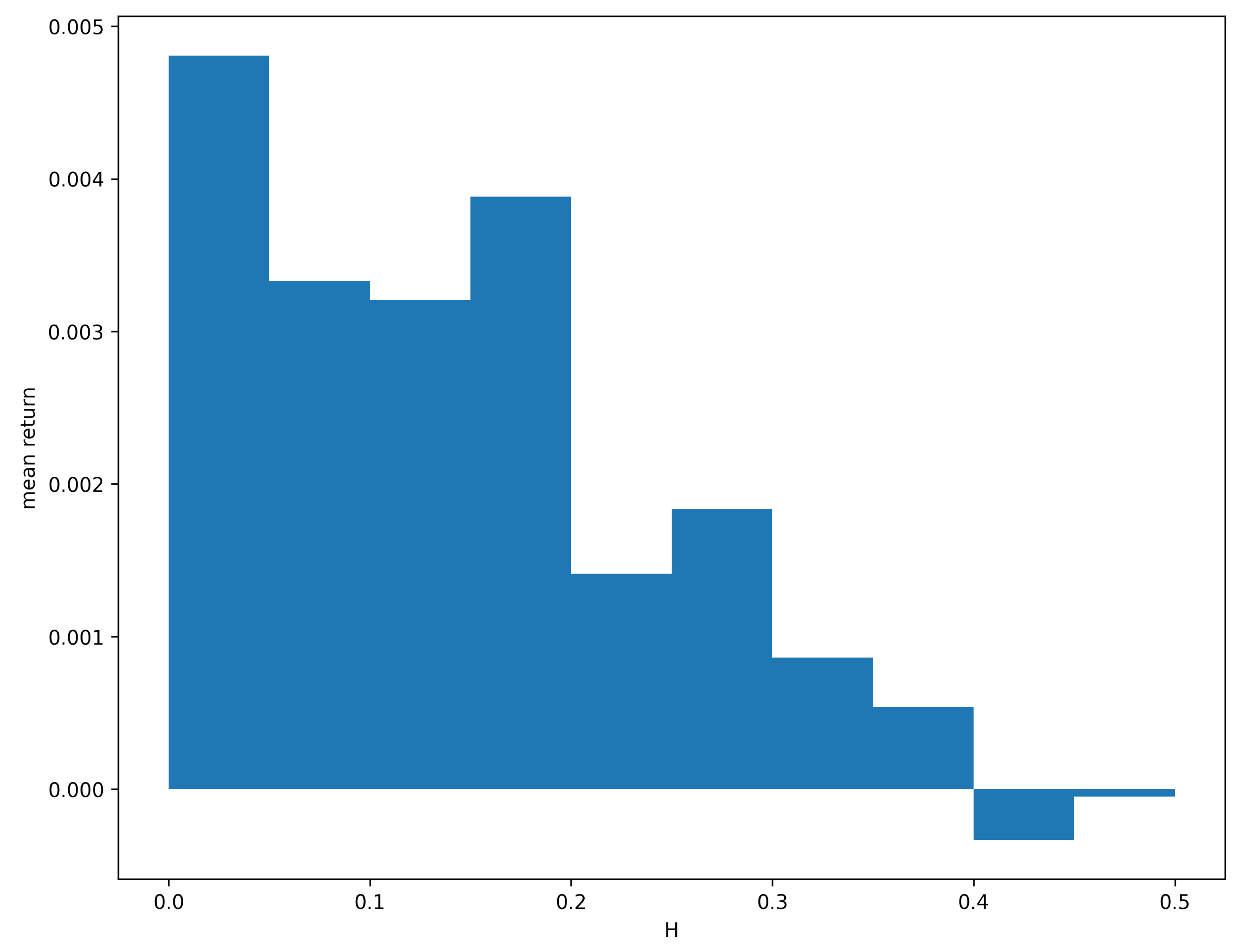
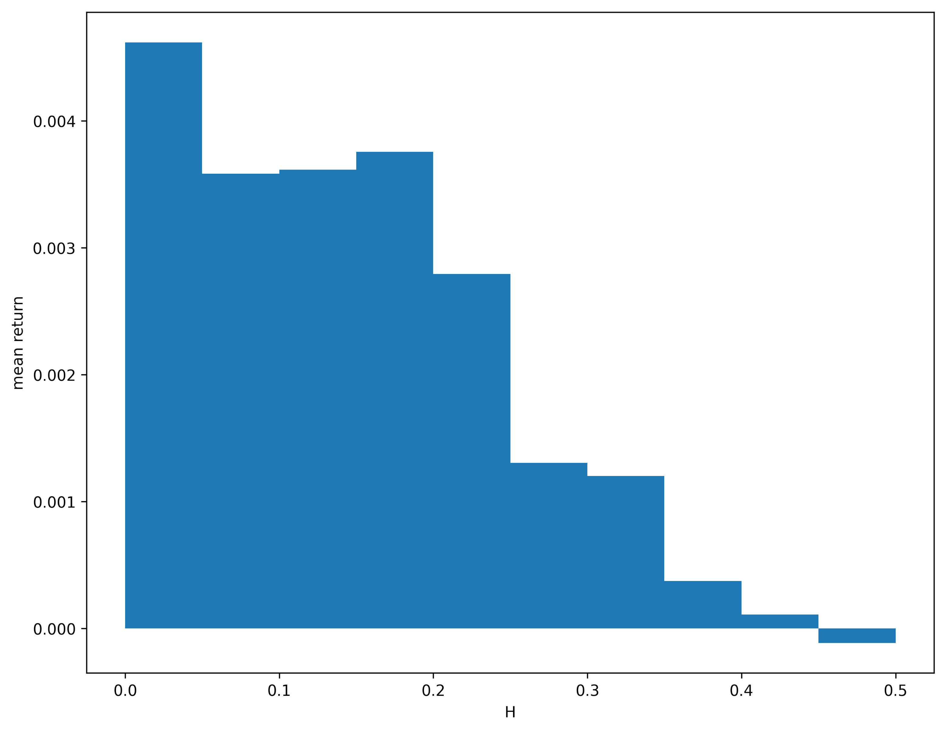
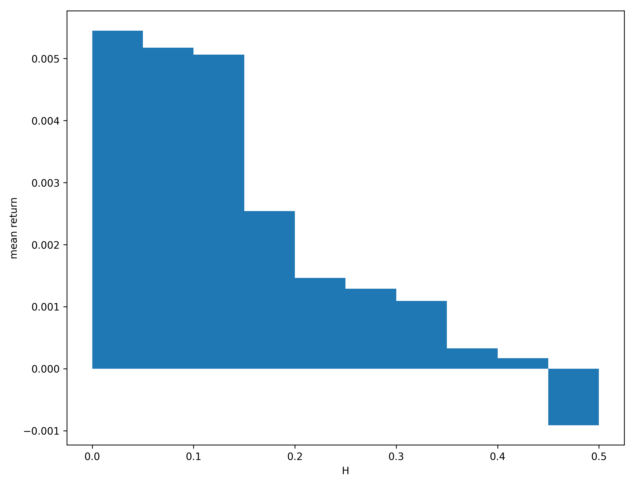
Figure 1, Figure 2 and Figure 3 show the relationship between the H value and the average return obtained for each of the periods studied (2000–07, 2007–14, 2014–20), in which all the countries considered in this paper are included. It can be seen that, as the value of H decreases, the average profitability increases for the three periods studied, it being significant that pairs with a value of 0.5 give negative average profitability. Therefore, those countries that select their pairs with an H close to 0 get a higher average return.
It is also important to note that the selection of the pairs based on the Hurst exponent is refreshed each six months with data from the previous year; therefore, the selected pairs are used for the next six months, without refreshing the calculation of the Hurst exponent. Consequently, these results are a kind of robustness check of the pair selection method, since we can see that the pairs with the lowest Hurst exponent in the past are the one for which the mean reversion strategy best work in the future.
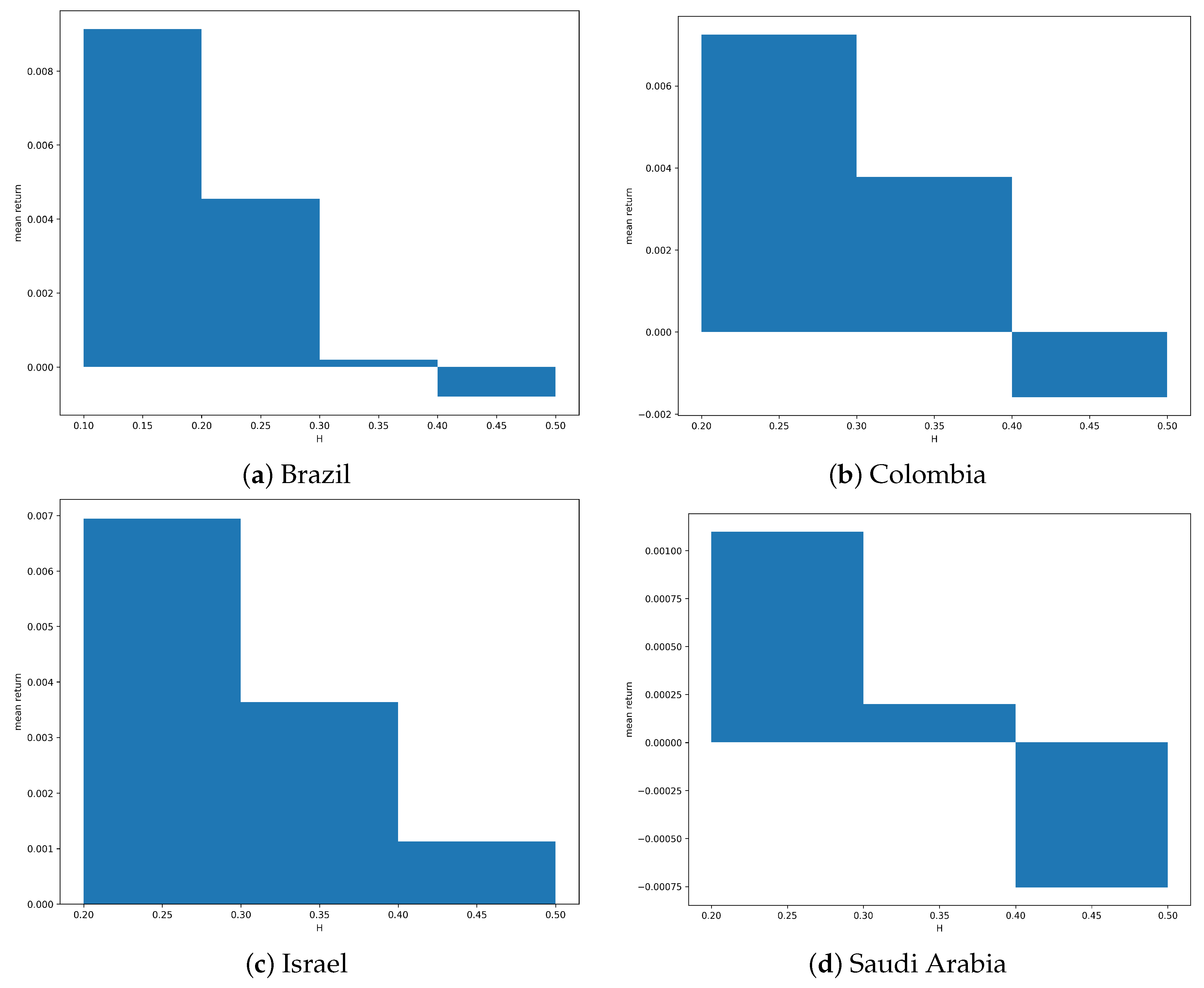
Figure 4 gives the relationship between the value of H and the average return for the period 2000–2007, for Brazil, Colombia, Israel, and Saudi Arabia. We can see that, in all cases, if only pairs with small values of H are selected, they would obtain their highest returns. The case of Brazil (a) is significant, as pairs with values between 0.1 and 0.2 would obtain an average return of around 1%. In the case of Brazil (a), Colombia (b), and Saudi Arabia (d), when the value of H of a pair is between 0.4 and 0.5, the strategy get negative returns.
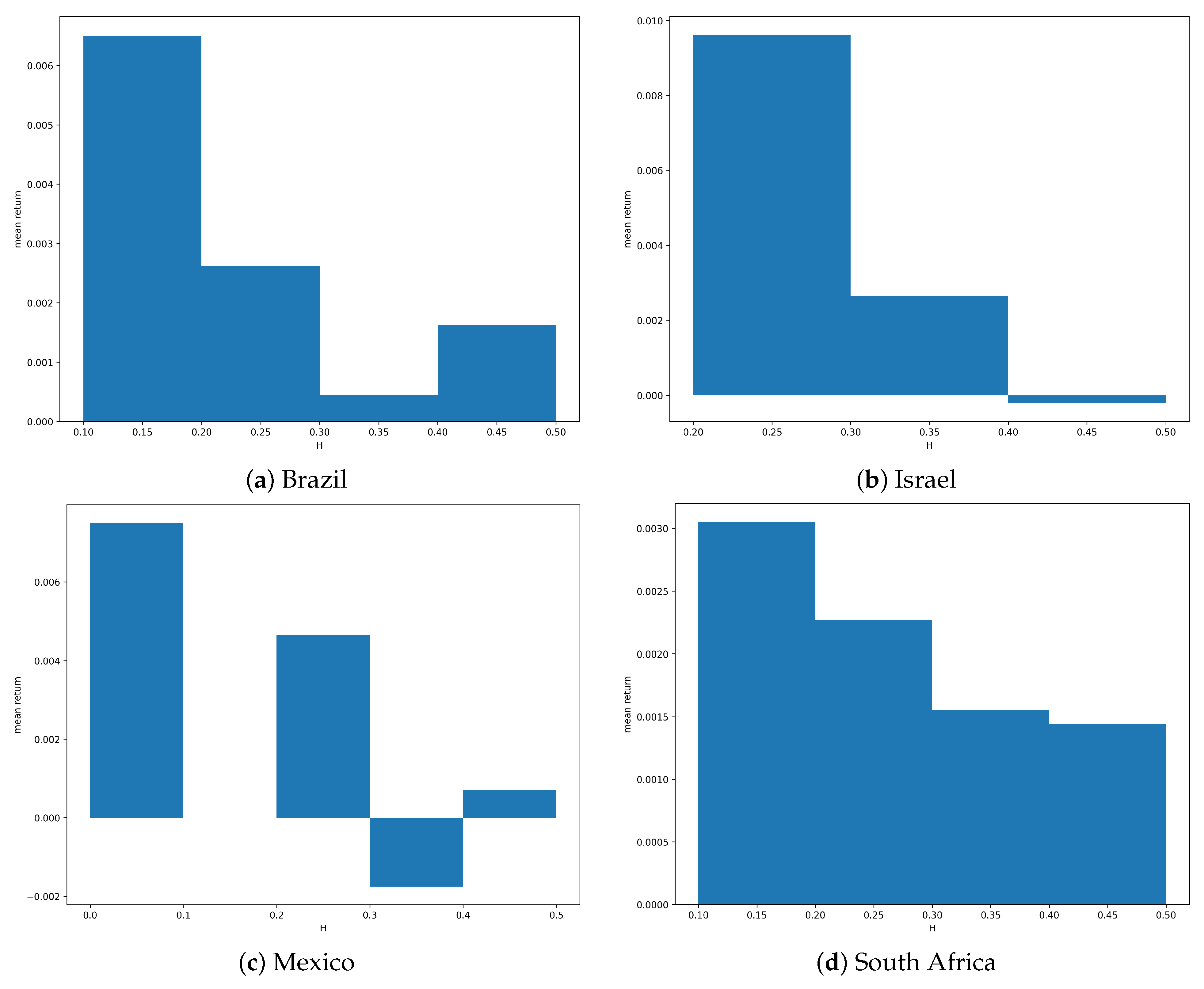
Figure 5 shows the comparison between average returns and the value of H, for the countries Brazil (a), Israel (b), Mexico (c), and South Africa (d) for the period 2007–2014. As in the previous period, as the value of H decreases, the average return increases. It is significant in the case of Brazil and South Africa that, for all the values of H, it obtains a positive profitability.
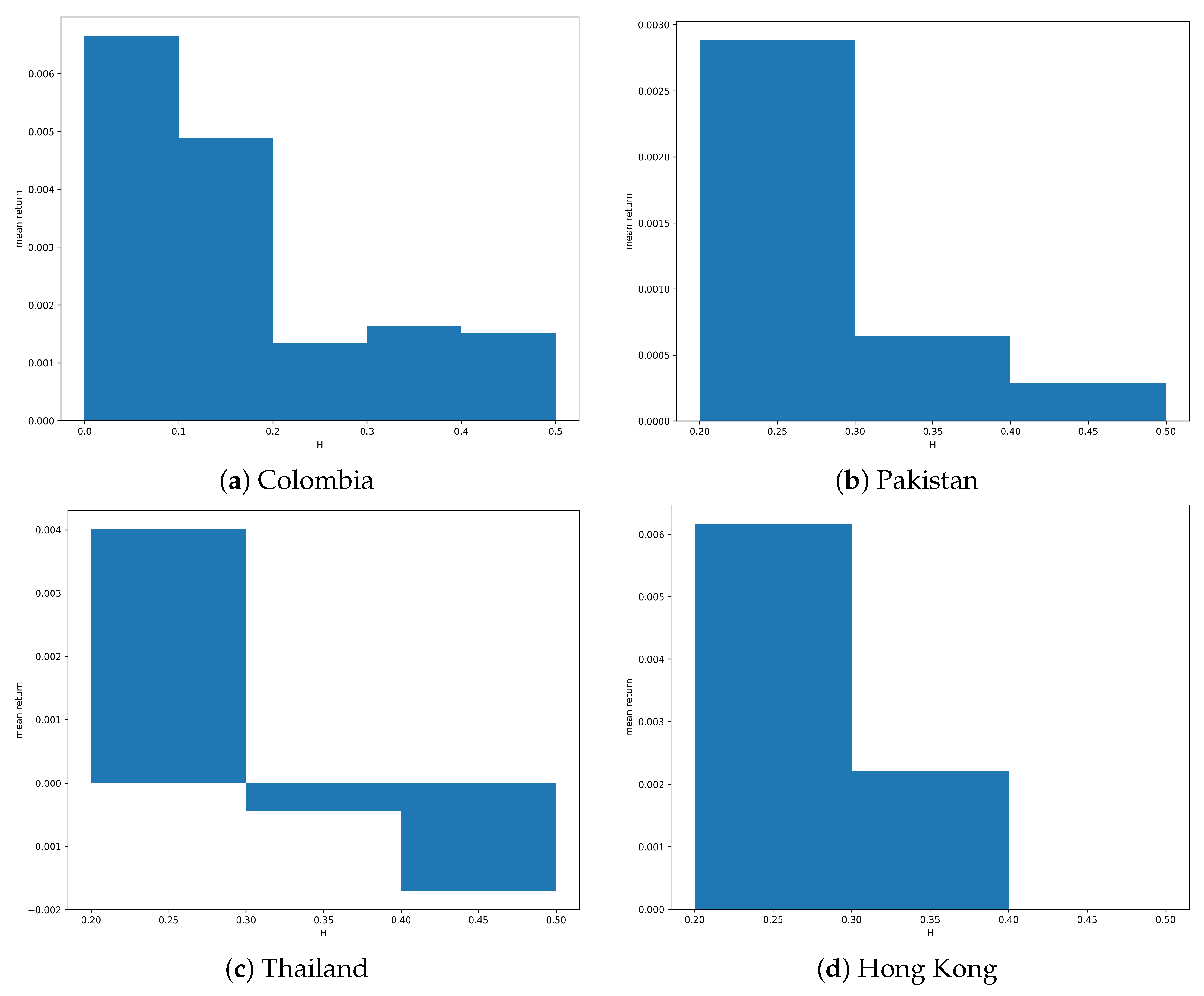
Finally, Figure 6 shows for Colombia (a), Pakistan (b), Thailand (c), and Hong Kong (d) the average profitability vs. the H value of the pair series for the period 2014–2020. As we have been seeing, as the value of the Hurst exponent (H) decreases, the average return increases. If we observe what happens in the case of Thailand, we would only obtain a positive average return if the value if H is between 0.2 and 0.3.
Therefore, we can also conclude that it is interesting to form the pairs of shares that make up the portfolios with the lowest possible value of the Hurst exponent of the pair series, as this would mean an increase in the profitability of the strategy.
4. Conclusions
According with the EMH, arbitrage strategies cannot over perform random portfolios with the same class of risk. In this paper, we look at market efficiency by comparing the performance of an arbitrage technique based on the Hurst exponent in emerging and developed markets.
We found that our statistical arbitrage strategy is consistent in emerging markets and it can obtain a significant profit during the period considered. This is the case of South Africa, Colombia, or Lebanon where the strategy obtains important results. However, in the case of the developed markets, only during high volatility periods, such as after the financial crisis, does the strategy performance properly. After the financial crisis, there are several markets where the Pairs Trading give significant results. The cases of Portugal and Greece are interesting, which are countries seriously affected by the financial crisis in Europe. These results are consistent with the previous findings of Ramos-Requena [35].
These results are also consistent with previous works of DiMatteo et al. [27], Zunino et al. [28], and Kristoufek [30], and they are a clear proof of the degree of inefficiency of emerging markets. Again, we consider that the performance of arbitrage methods in developed markets during specific periods could be considered a proof of the Adaptative Markets hypothesis [64].
On the other hand, we have studied the degree of incidence that the value of the Hurst exponent of the pair series has on the strategy performance, as proposed by Ramos-Requena et al. [35]. We have proved that the main characteristics of the Pairs Trading strategy, the mean reversion, are achieved with a low H. Another interesting result is that, when the value of H is around 0.1 or 0.2, the performance of the strategy is greater.
To conclude, we would like to remark that the selection methodology shows that the strategy is robust because the pairs with the lowest Hurst exponent in the past are the one for which the mean reversion strategy best works in the future.
Next, we highlight some possible limitations of this study (we thank the anonymous referees for pointing these out). The main issue is that the inefficiency of some markets may be due to various market frictions. For example, short selling banning on some countries is not taken into consideration for the difficulties to short sell some stocks in some countries. We have considered transaction fees, but we have not considered any cost or revenue incurring by the short selling positions, as well as any revenue for interest on cash not used. We have used daily closing prices to open or close positions. Though we have considered the most capitalized stocks in each country, it is still possible that the scale of the strategy may impact those prices. Therefore, the real implementation of this strategy may suffer some difficulties and the profitability of the strategy may be lower due to market frictions. However, we are mainly interested in the inefficiency of the markets, and it is beyond the scope of this paper (though very interesting) to determine the origin of this inefficiency.
.
Author Contributions
Conceptualization, K.B., J.P.R.-R., J.E.T.-S., and M.A.S.-G.; Methodology, K.B., J.P.R.-R., J.E.T.-S., and M.A.S.-G.; Software, K.B., J.P.R.-R., J.E.T.-S., and M.A.S.-G.; Validation, K.B., J.P.R.-R., J.E.T.-S., and M.A.S.-G.; Formal Analysis, K.B., J.P.R.-R., J.E.T.-S., and M.A.S.-G.; Investigation, K.B., J.P.R.-R., J.E.T.-S., and M.A.S.-G.; Resources, K.B., J.P.R.-R., J.E.T.-S., and M.A.S.-G.; Data Curation, K.B., J.P.R.-R., J.E.T.-S., and M.A.S.-G.; Writing—Original Draft Preparation, K.B., J.P.R.-R., J.E.T.-S., and M.A.S.-G.; Writing—Review and Editing, K.B., J.P.R.-R., J.E.T.-S., and M.A.S.-G.; Visualization, K.B., J.P.R.-R., J.E.T.-S., and M.A.S.-G.; Supervision, K.B., J.P.R.-R., J.E.T.-S., and M.A.S.-G.; Project Administration, K.B., J.P.R.-R., J.E.T.-S., and M.A.S.-G.; Funding Acquisition, J.E.T.-S. and M.A.S.-G. All authors have read and agreed to the published version of the manuscript.
Funding
Juan Evangelista Trinidad-Segovia is supported by grant PGC2018-101555-B-I00 (Ministerio Español de Ciencia, Innovación y Universidades and FEDER) and UAL18-FQM-B038-A (UAL/CECEU/FEDER). Miguel Ángel Sánchez-Granero acknowledges the support of grants PGC2018-101555-B-I00 (Ministerio Español de Ciencia, Innovación y Universidades and FEDER) and UAL18-FQM-B038-A (UAL/CECEU/FEDER) and CDTIME.
Institutional Review Board Statement
Not applicable.
Informed Consent Statement
Not applicable.
Data Availability Statement
Publicly available datasets were analyzed in this study. This data can be found here: Investing.com.
Conflicts of Interest
The authors declare no conflict of interest.
Appendix A. Classification of Emerging and Advanced Countries

Table A1.
Classification of emerging and advanced countries (following MSCI).
| Country | Classification |
|---|---|
| Argentina | Emerging |
| Bahrain | Emerging |
| Belgium | Advanced |
| Brazil | Emerging |
| Colombia | Emerging |
| Czech Republic | Emerging |
| Denmark | Advanced |
| Dubai | Emerging |
| Finland | Advanced |
| France | Advanced |
| Greece | Emerging |
| Hong Kong | Advanced |
| India | Emerging |
| Israel | Advanced |
| Italy | Advanced |
| Japan | Advanced |
| Jordan | Emerging |
| Kuwait | Emerging |
| Lebanon | Emerging |
| Mauritius | Emerging |
| Mexico | Emerging |
| Morocco | Emerging |
| Namibia | Emerging |
| Netherlands | Advanced |
| Norway | Advanced |
| Oman | Emerging |
| Pakistan | Emerging |
| Palestine | Emerging |
| Poland | Emerging |
| Portugal | Advanced |
| Romania | Emerging |
| Russia | Emerging |
| Saudi Arabia | Emerging |
| South Africa | Emerging |
| Spain | Advanced |
| Sweden | Advanced |
| Switzerland | Advanced |
| Thailand | Emerging |
| United States | Advanced |
Appendix B. Results
Below is a comparison between the main results obtained.
Appendix B.1. Period 2000–2007
Table A2.
Results obtained for the period 2000–2007 (30 Pairs), where N is the number of pairs; AAV Average annualized return; and Profit is the profitability for the full period with transaction costs.
Table A2.
Results obtained for the period 2000–2007 (30 Pairs), where N is the number of pairs; AAV Average annualized return; and Profit is the profitability for the full period with transaction costs.
| Country | N | Operations | AAV | Sharpe Ratio | Profits |
|---|---|---|---|---|---|
| Argentina | 30 | 1666 | 0.80% | 0.31 | 4.14% |
| Bahrain | 30 | 6 | −0.10% | −0.53 | −0.20% |
| Belgium | 30 | 3617 | 1.50% | 0.57 | 10.99% |
| Brazil | 30 | 3127 | 1.10% | 0.26 | 7.06% |
| Colombia | 30 | 1612 | −0.80% | −0.25 | −4.34% |
| Czech Republic | 30 | 1224 | −0.40% | −0.26 | −3.31% |
| Denmark | 30 | 2710 | −0.30% | −0.11 | −2.60% |
| Dubai | 30 | 509 | −0.50% | −0.30 | −2.67% |
| Finland | 30 | 2591 | 2.00% | 0.72 | 14.64% |
| France | 30 | 3284 | 1.50% | 0.54 | 11.71% |
| Greece | 30 | 2644 | 0.20% | 0.05 | 0.32% |
| Hong Kong | 30 | 63 | 0.20% | 0.78 | 1.28% |
| India | 30 | 3116 | 0.80% | 0.22 | 5.46% |
| Israel | 30 | 3628 | 3.60% | 0.96 | 28.99% |
| Italy | 30 | 3249 | 1.80% | 0.68 | 13.22% |
| Japan | 30 | 2983 | 4.00% | 1.04 | 32.61% |
| Jordan | 30 | 1980 | 0.50% | 0.16 | 2.14% |
| Kuwait | 30 | 2452 | 0.20% | 0.07 | 0.58% |
| Lebanon | 30 | 171 | 0.60% | 1.11 | 2.64% |
| Mauritius | 30 | 1855 | −0.50% | −0.23 | −3.92% |
| Mexico | 30 | 2362 | 1.40% | 0.48 | 7.91% |
| Morocco | 30 | 882 | 0.60% | 0.35 | 3.91% |
| Namibia | 30 | 1590 | 3.00% | 1.06 | 12.07% |
| Netherlands | 30 | 3322 | 3.20% | 0.80 | 27.59% |
| Norway | 30 | 679 | −1.10% | −0.74 | −8.63% |
| Oman | 30 | 740 | −0.10% | −0.08 | −0.85% |
| Pakistan | 30 | 2116 | 1.90% | 0.51 | 14.19% |
| Palestine | 30 | 264 | 0.50% | 0.42 | 2.51% |
| Poland | 30 | 4 | 0.90% | 1.37 | 0.20% |
| Portugal | 30 | 2772 | −0.50% | −0.16 | −4.72% |
| Romania | 30 | 34 | −0.30% | −0.71 | −1.21% |
| Russia | 30 | 2887 | −0.90% | −0.27 | −7.86% |
| Saudi Arabia | 30 | 2530 | 0.30% | 0.12 | 1.86% |
| South Africa | 30 | 4682 | 6.90% | 1.45 | 65.84% |
| Spain | 30 | 304 | 0.00% | −0.07 | −0.40% |
| Sweden | 30 | 4057 | 0.00% | −0.01 | −1.55% |
| Switzerland | 30 | 3552 | 0.60% | 0.19 | 3.32% |
| Thailand | 30 | 2779 | 0.80% | 0.21 | 4.77% |
| United States | 30 | 2736 | −1.50% | −0.26 | −11.61% |
Table A3.
Results obtained for the period 2000–2007 (40 Pairs), where N is the number of pairs; AAV Average annualized return; and Profit is the profitability for the full period with transaction costs.
Table A3.
Results obtained for the period 2000–2007 (40 Pairs), where N is the number of pairs; AAV Average annualized return; and Profit is the profitability for the full period with transaction costs.
| Country | N | Operations | AAV | Sharpe Ratio | Profits |
|---|---|---|---|---|---|
| Argentina | 40 | 1776 | 0.50% | 0.27 | 2.66% |
| Bahrain | 40 | 6 | −0.10% | −0.53 | −0.20% |
| Belgium | 40 | 4714 | 1.40% | 0.61 | 10.12% |
| Brazil | 40 | 3923 | 0.40% | 0.12 | 2.32% |
| Colombia | 40 | 1851 | −0.50% | −0.18 | −2.76% |
| Czech Republic | 40 | 1224 | −0.30% | −0.26 | −2.51% |
| Denmark | 40 | 3477 | −0.20% | −0.10 | −2.27% |
| Dubai | 40 | 509 | −0.40% | −0.30 | −2.03% |
| Finland | 40 | 3393 | 2.10% | 0.78 | 15.15% |
| France | 40 | 4158 | 1.70% | 0.67 | 12.96% |
| Greece | 40 | 3499 | −0.20% | −0.04 | −1.87% |
| Hong Kong | 40 | 63 | 0.10% | 0.78 | 0.98% |
| India | 40 | 4084 | 0.90% | 0.25 | 6.18% |
| Israel | 40 | 4658 | 3.00% | 0.91 | 23.54% |
| Italy | 40 | 4124 | 1.80% | 0.77 | 13.47% |
| Japan | 40 | 3795 | 3.60% | 1.02 | 29.45% |
| Jordan | 40 | 2539 | −0.10% | −0.03 | −1.13% |
| Kuwait | 40 | 3204 | 0.20% | 0.09 | 1.00% |
| Lebanon | 40 | 171 | 0.40% | 1.11 | 2.06% |
| Mauritius | 40 | 2335 | −0.50% | −0.28 | −4.08% |
| Mexico | 40 | 3032 | 0.50% | 0.19 | 2.24% |
| Morocco | 40 | 1018 | 0.40% | 0.32 | 3.15% |
| Namibia | 40 | 1706 | 2.50% | 1.10 | 10.17% |
| Netherlands | 40 | 4486 | 3.40% | 0.95 | 28.78% |
| Norway | 40 | 679 | −0.80% | −0.74 | −6.47% |
| Oman | 40 | 809 | 0.10% | 0.07 | 0.20% |
| Pakistan | 40 | 2620 | 2.00% | 0.65 | 15.54% |
| Palestine | 40 | 264 | 0.40% | 0.42 | 1.83% |
| Poland | 40 | 4 | 0.70% | 1.37 | 0.10% |
| Portugal | 40 | 3710 | −0.30% | −0.11 | −3.43% |
| Romania | 40 | 34 | −0.20% | −0.71 | −0.91% |
| Russia | 40 | 3503 | −1.00% | −0.33 | −8.58% |
| Saudi Arabia | 40 | 3320 | 0.00% | 0.00 | −0.73% |
| South Africa | 40 | 6073 | 6.90% | 1.60 | 65.68% |
| Spain | 40 | 304 | 0.00% | −0.07 | −0.28% |
| Sweden | 40 | 5049 | −0.40% | −0.16 | −4.26% |
| Switzerland | 40 | 4734 | 0.30% | 0.12 | 1.32% |
| Thailand | 40 | 3589 | 0.00% | 0.00 | −0.90% |
| United States | 40 | 3461 | −1.70% | −0.35 | −12.87% |
Table A4.
Results obtained for the period 2000–2007 (50 Pairs), where N is the number of pairs; AAV Average annualized return; and Profit is the profitability for the full period with transaction costs.
Table A4.
Results obtained for the period 2000–2007 (50 Pairs), where N is the number of pairs; AAV Average annualized return; and Profit is the profitability for the full period with transaction costs.
| Country | N | Operations | AAV | Sharpe Ratio | Profits |
|---|---|---|---|---|---|
| Argentina | 50 | 1776 | 0.40% | 0.27 | 2.14% |
| Bahrain | 50 | 6 | −0.10% | −0.53 | −0.10% |
| Belgium | 50 | 5735 | 1.40% | 0.66 | 10.25% |
| Brazil | 50 | 4747 | 0.90% | 0.24 | 5.65% |
| Colombia | 50 | 2080 | −0.50% | −0.20 | −2.72% |
| Czech Republic | 50 | 1224 | −0.20% | −0.26 | −2.04% |
| Denmark | 50 | 4307 | −0.20% | −0.09 | −2.06% |
| Dubai | 50 | 509 | −0.30% | −0.30 | −1.60% |
| Finland | 50 | 4213 | 1.90% | 0.76 | 13.96% |
| France | 50 | 4987 | 1.80% | 0.77 | 13.80% |
| Greece | 50 | 4315 | −0.40% | −0.14 | −3.66% |
| Hong Kong | 50 | 63 | 0.10% | 0.78 | 0.79% |
| India | 50 | 4870 | 0.90% | 0.28 | 6.23% |
| Israel | 50 | 5710 | 3.30% | 1.09 | 25.76% |
| Italy | 50 | 4973 | 1.60% | 0.75 | 12.21% |
| Japan | 50 | 4637 | 3.60% | 1.08 | 28.87% |
| Jordan | 50 | 3071 | 0.20% | 0.08 | 0.59% |
| Kuwait | 50 | 3904 | 0.20% | 0.09 | 0.82% |
| Lebanon | 50 | 171 | 0.30% | 1.11 | 1.57% |
| Mauritius | 50 | 2782 | −0.50% | −0.34 | −4.16% |
| Mexico | 50 | 3573 | 0.50% | 0.23 | 2.59% |
| Morocco | 50 | 1144 | 0.40% | 0.28 | 2.47% |
| Namibia | 50 | 1706 | 2.00% | 1.10 | 8.16% |
| Netherlands | 50 | 5586 | 3.10% | 0.96 | 26.08% |
| Norway | 50 | 679 | −0.70% | −0.74 | −5.24% |
| Oman | 50 | 828 | 0.00% | 0.03 | −0.07% |
| Pakistan | 50 | 2989 | 1.90% | 0.69 | 14.50% |
| Palestine | 50 | 264 | 0.30% | 0.42 | 1.55% |
| Poland | 50 | 4 | 0.50% | 1.37 | 0.10% |
| Portugal | 50 | 4643 | −0.60% | −0.23 | −5.43% |
| Romania | 50 | 34 | −0.20% | −0.71 | −0.71% |
| Russia | 50 | 4114 | −0.60% | −0.21 | −5.52% |
| Saudi Arabia | 50 | 4075 | 0.00% | −0.01 | −1.12% |
| South Africa | 50 | 7458 | 7.40% | 1.98 | 71.21% |
| Spain | 50 | 304 | 0.00% | −0.07 | −0.26% |
| Sweden | 50 | 5989 | −0.50% | −0.21 | −4.90% |
| Switzerland | 50 | 5847 | 0.50% | 0.19 | 2.63% |
| Thailand | 50 | 4179 | 0.10% | 0.05 | 0.16% |
| United States | 50 | 4180 | −1.30% | −0.31 | −10.04% |
Appendix B.2. Period 2007–2014
Table A5.
Results obtained for the period 2007–2014 (30 Pairs), where N is the number of pairs; AAV Average annualized return; and Profit is the profitability for the full period with transaction costs.
Table A5.
Results obtained for the period 2007–2014 (30 Pairs), where N is the number of pairs; AAV Average annualized return; and Profit is the profitability for the full period with transaction costs.
| Country | N | Operations | AAV | Sharpe Ratio | Profits |
|---|---|---|---|---|---|
| Argentina | 30 | 2877 | 0.10% | 0.03 | −0.06% |
| Bahrain | 30 | 186 | 0.90% | 1.04 | 4.94% |
| Belgium | 30 | 4076 | 2.90% | 0.92 | 23.64% |
| Brazil | 30 | 3756 | 2.00% | 0.53 | 14.55% |
| Colombia | 30 | 3844 | 1.00% | 0.41 | 6.62% |
| Czech Republic | 30 | 506 | 1.30% | 0.52 | 9.93% |
| Denmark | 30 | 3024 | 1.70% | 0.40 | 12.69% |
| Dubai | 30 | 2836 | −2.00% | −0.56 | −15.25% |
| Finland | 30 | 4103 | 2.00% | 0.48 | 15.03% |
| France | 30 | 3470 | 1.50% | 0.48 | 10.94% |
| Greece | 30 | 3739 | 2.50% | 0.48 | 19.85% |
| Hong Kong | 30 | 1425 | 1.70% | 0.55 | 5.72% |
| India | 30 | 4051 | 3.20% | 0.51 | 25.75% |
| Israel | 30 | 3735 | 6.10% | 1.23 | 54.25% |
| Italy | 30 | 3817 | 1.80% | 0.52 | 13.83% |
| Japan | 30 | 3010 | 3.70% | 0.84 | 30.30% |
| Jordan | 30 | 2359 | 0.60% | 0.15 | 3.41% |
| Kuwait | 30 | 2862 | −0.10% | −0.03 | −1.85% |
| Lebanon | 30 | 318 | 0.70% | 2.53 | 5.39% |
| Mauritius | 30 | 1153 | 0.40% | 0.28 | 2.72% |
| Mexico | 30 | 2535 | 1.00% | 0.34 | 7.35% |
| Morocco | 30 | 2635 | 0.60% | 0.23 | 3.82% |
| Namibia | 30 | 2537 | 1.60% | 0.50 | 11.95% |
| Netherlands | 30 | 3415 | 3.10% | 0.71 | 26.26% |
| Norway | 30 | 2091 | −0.90% | −0.41 | −7.50% |
| Oman | 30 | 1816 | −1.30% | −0.57 | −10.11% |
| Pakistan | 30 | 2805 | 0.80% | 0.16 | 5.06% |
| Palestine | 30 | 492 | −0.60% | −0.69 | −4.56% |
| Poland | 30 | 1886 | 1.80% | 0.88 | 13.37% |
| Portugal | 30 | 3836 | 4.20% | 0.73 | 36.82% |
| Romania | 30 | 723 | 2.50% | 0.83 | 19.76% |
| Russia | 30 | 3081 | 0.70% | 0.15 | 4.27% |
| Saudi Arabia | 30 | 3508 | 0.50% | 0.14 | 2.33% |
| South Africa | 30 | 4557 | 3.60% | 1.08 | 29.88% |
| Spain | 30 | 2087 | 0.20% | 0.07 | 0.80% |
| Sweden | 30 | 4072 | 2.50% | 0.55 | 19.14% |
| Switzerland | 30 | 4033 | 2.90% | 0.79 | 22.86% |
| Thailand | 30 | 3217 | −1.10% | −0.27 | −8.67% |
| United States | 30 | 2996 | 0.30% | 0.11 | 1.30% |
Table A6.
Results obtained for the period 2007–2014 (40 Pairs), where N is the number of pairs; AAV Average annualized return; and Profit is the profitability for the full period with transaction costs.
Table A6.
Results obtained for the period 2007–2014 (40 Pairs), where N is the number of pairs; AAV Average annualized return; and Profit is the profitability for the full period with transaction costs.
| Country | N | Operations | AAV | Sharpe Ratio | Profits |
|---|---|---|---|---|---|
| Argentina | 40 | 3660 | 0.20% | 0.05 | 0.48% |
| Bahrain | 40 | 186 | 0.70% | 1.04 | 3.65% |
| Belgium | 40 | 5243 | 2.50% | 0.87 | 20.29% |
| Brazil | 40 | 4796 | 2.20% | 0.67 | 16.60% |
| Colombia | 40 | 4846 | 0.70% | 0.32 | 4.19% |
| Czech Republic | 40 | 506 | 1.00% | 0.52 | 7.37% |
| Denmark | 40 | 4008 | 0.90% | 0.23 | 6.20% |
| Dubai | 40 | 3524 | −1.40% | −0.43 | −11.28% |
| Finland | 40 | 5308 | 1.80% | 0.46 | 13.47% |
| France | 40 | 4551 | 1.20% | 0.42 | 8.56% |
| Greece | 40 | 4873 | 2.50% | 0.53 | 19.88% |
| Hong Kong | 40 | 1831 | 1.00% | 0.35 | 3.34% |
| India | 40 | 5287 | 3.60% | 0.63 | 29.78% |
| Israel | 40 | 4858 | 5.90% | 1.35 | 51.59% |
| Italy | 40 | 4841 | 2.30% | 0.77 | 18.49% |
| Japan | 40 | 3919 | 3.00% | 0.72 | 23.12% |
| Jordan | 40 | 3023 | 0.70% | 0.18 | 4.14% |
| Kuwait | 40 | 3839 | −0.10% | −0.02 | −1.36% |
| Lebanon | 40 | 318 | 0.50% | 2.53 | 4.02% |
| Mauritius | 40 | 1317 | 0.30% | 0.20 | 1.67% |
| Mexico | 40 | 3283 | 0.70% | 0.25 | 4.48% |
| Morocco | 40 | 3307 | 0.60% | 0.27 | 3.97% |
| Namibia | 40 | 3004 | 1.50% | 0.57 | 10.95% |
| Netherlands | 40 | 4517 | 3.60% | 0.91 | 31.27% |
| Norway | 40 | 2536 | −0.80% | −0.40 | −6.43% |
| Oman | 40 | 2395 | −1.10% | −0.52 | −8.50% |
| Pakistan | 40 | 3607 | 1.40% | 0.31 | 9.70% |
| Palestine | 40 | 492 | −0.50% | −0.69 | −3.42% |
| Poland | 40 | 2435 | 1.60% | 0.82 | 11.59% |
| Portugal | 40 | 4981 | 3.00% | 0.62 | 24.75% |
| Romania | 40 | 889 | 2.10% | 0.90 | 16.88% |
| Russia | 40 | 3996 | 1.20% | 0.30 | 8.70% |
| Saudi Arabia | 40 | 4594 | 0.80% | 0.27 | 4.85% |
| South Africa | 40 | 6004 | 4.00% | 1.28 | 33.80% |
| Spain | 40 | 2678 | 0.50% | 0.20 | 3.33% |
| Sweden | 40 | 5126 | 2.00% | 0.49 | 15.12% |
| Switzerland | 40 | 5175 | 1.70% | 0.55 | 12.71% |
| Thailand | 40 | 4267 | −0.90% | −0.27 | −7.87% |
| United States | 40 | 3882 | 0.70% | 0.28 | 4.13% |
Table A7.
Results obtained for the period 2007–2014 (50 Pairs), where N is the number of pairs; AAV Average annualized return; and Profit is the profitability for the full period with transaction costs.
Table A7.
Results obtained for the period 2007–2014 (50 Pairs), where N is the number of pairs; AAV Average annualized return; and Profit is the profitability for the full period with transaction costs.
| Country | N | Operations | AAV | Sharpe Ratio | Profits |
|---|---|---|---|---|---|
| Argentina | 50 | 4279 | −0.20% | −0.06 | −2.16% |
| Bahrain | 50 | 186 | 0.50% | 1.04 | 2.96% |
| Belgium | 50 | 6496 | 3.10% | 1.14 | 25.60% |
| Brazil | 50 | 5854 | 2.40% | 0.79 | 18.43% |
| Colombia | 50 | 5762 | 0.70% | 0.34 | 4.05% |
| Czech Republic | 50 | 506 | 0.80% | 0.52 | 5.90% |
| Denmark | 50 | 4884 | 0.90% | 0.25 | 6.32% |
| Dubai | 50 | 4144 | −1.20% | −0.40 | −10.03% |
| Finland | 50 | 6471 | 1.80% | 0.51 | 13.51% |
| France | 50 | 5527 | 1.30% | 0.49 | 9.89% |
| Greece | 50 | 6049 | 2.50% | 0.57 | 19.89% |
| Hong Kong | 50 | 2218 | 1.10% | 0.41 | 3.76% |
| India | 50 | 6529 | 3.20% | 0.60 | 25.79% |
| Israel | 50 | 5917 | 5.50% | 1.44 | 47.32% |
| Italy | 50 | 5987 | 2.80% | 0.99 | 23.10% |
| Japan | 50 | 4813 | 2.50% | 0.64 | 18.94% |
| Jordan | 50 | 3703 | 0.60% | 0.22 | 4.06% |
| Kuwait | 50 | 4698 | 0.60% | 0.23 | 4.16% |
| Lebanon | 50 | 318 | 0.40% | 2.53 | 3.14% |
| Mauritius | 50 | 1493 | 0.20% | 0.14 | 1.10% |
| Mexico | 50 | 3921 | 0.60% | 0.23 | 3.72% |
| Morocco | 50 | 3965 | 0.40% | 0.20 | 2.31% |
| Namibia | 50 | 3395 | 1.30% | 0.59 | 9.62% |
| Netherlands | 50 | 5798 | 3.30% | 0.92 | 27.94% |
| Norway | 50 | 2941 | −0.80% | −0.48 | −6.59% |
| Oman | 50 | 2805 | −1.00% | −0.49 | −7.46% |
| Pakistan | 50 | 4395 | 1.40% | 0.37 | 9.92% |
| Palestine | 50 | 492 | −0.40% | −0.69 | −2.80% |
| Poland | 50 | 2935 | 1.50% | 0.84 | 10.91% |
| Portugal | 50 | 6108 | 3.00% | 0.70 | 24.88% |
| Romania | 50 | 1045 | 1.80% | 0.88 | 14.09% |
| Russia | 50 | 4998 | 1.20% | 0.33 | 8.40% |
| Saudi Arabia | 50 | 5611 | 0.90% | 0.34 | 6.08% |
| South Africa | 50 | 7346 | 3.90% | 1.31 | 32.73% |
| Spain | 50 | 3100 | 0.30% | 0.15 | 1.98% |
| Sweden | 50 | 6263 | 2.30% | 0.62 | 17.45% |
| Switzerland | 50 | 6294 | 2.00% | 0.73 | 15.54% |
| Thailand | 50 | 5249 | −1.40% | −0.45 | −11.05% |
| United States | 50 | 4723 | 0.70% | 0.32 | 4.66% |
Appendix B.3. Period 2014–2020
Table A8.
Results obtained for the period 2014–2020 (30 Pairs), where N is the number of pairs; AAV Average annualized return; and Profit is the profitability for the full period with transaction costs.
Table A8.
Results obtained for the period 2014–2020 (30 Pairs), where N is the number of pairs; AAV Average annualized return; and Profit is the profitability for the full period with transaction costs.
| Country | N | Operations | AAV | Sharpe Ratio | Profits |
|---|---|---|---|---|---|
| Argentina | 30 | 2514 | 0.00% | 0.00 | −0.94% |
| Bahrain | 30 | 5 | 0.00% | 0.16 | 0.00% |
| Belgium | 30 | 3048 | 3.90% | 1.82 | 24.98% |
| Brazil | 30 | 2375 | 2.40% | 0.70 | 13.61% |
| Colombia | 30 | 3543 | 5.00% | 2.11 | 31.02% |
| Czech Republic | 30 | 1009 | −0.70% | −0.48 | −4.44% |
| Denmark | 30 | 2089 | 1.30% | 0.56 | 7.10% |
| Dubai | 30 | 2307 | −1.30% | −0.35 | −7.87% |
| Finland | 30 | 3001 | 0.90% | 0.30 | 4.30% |
| France | 30 | 2411 | −0.60% | −0.31 | −4.20% |
| Greece | 30 | 2978 | 8.60% | 1.35 | 59.71% |
| Hong Kong | 30 | 1997 | 2.20% | 0.57 | 11.43% |
| India | 30 | 2760 | 2.50% | 0.47 | 14.38% |
| Israel | 30 | 2590 | 1.40% | 0.71 | 7.64% |
| Italy | 30 | 2687 | 1.40% | 0.55 | 7.60% |
| Japan | 30 | 2108 | 1.90% | 0.60 | 10.60% |
| Jordan | 30 | 1682 | −0.30% | −0.17 | −2.46% |
| Kuwait | 30 | 2834 | 2.70% | 0.85 | 15.36% |
| Lebanon | 30 | 182 | 1.30% | 3.85 | 7.04% |
| Mauritius | 30 | 233 | 0.00% | 0.08 | 0.12% |
| Mexico | 30 | 1808 | −1.40% | −0.67 | −8.90% |
| Morocco | 30 | 1606 | 0.20% | 0.12 | 0.76% |
| Namibia | 30 | 2260 | 2.00% | 0.71 | 11.55% |
| Netherlands | 30 | 2467 | 1.70% | 0.59 | 9.58% |
| Norway | 30 | 2381 | 0.80% | 0.29 | 4.41% |
| Oman | 30 | 1005 | −0.20% | −0.12 | −1.44% |
| Pakistan | 30 | 2149 | 1.00% | 0.25 | 5.28% |
| Palestine | 30 | 358 | 0.00% | 0.04 | −0.02% |
| Poland | 30 | 2804 | 2.00% | 0.65 | 11.47% |
| Portugal | 30 | 2243 | 0.00% | 0.01 | −0.55% |
| Romania | 30 | 2036 | 0.50% | 0.15 | 2.22% |
| Russia | 30 | 2095 | 0.00% | −0.01 | −0.90% |
| Saudi Arabia | 30 | 2780 | 2.60% | 0.82 | 14.77% |
| South Africa | 30 | 3036 | 3.90% | 1.27 | 23.79% |
| Spain | 30 | 2321 | −0.80% | −0.28 | −5.37% |
| Sweden | 30 | 2653 | 2.60% | 1.05 | 15.82% |
| Switzerland | 30 | 2259 | 0.80% | 0.32 | 4.35% |
| Thailand | 30 | 1869 | 0.00% | 0.01 | −0.52% |
| United States | 30 | 2090 | 0.80% | 0.41 | 4.20% |
Table A9.
Results obtained for the period 2014–2020 (40 Pairs), where N is the number of pairs; AAV Average annualized return; and Profit is the profitability for the full period with transaction costs.
Table A9.
Results obtained for the period 2014–2020 (40 Pairs), where N is the number of pairs; AAV Average annualized return; and Profit is the profitability for the full period with transaction costs.
| Country | N | Operations | AAV | Sharpe Ratio | Profits |
|---|---|---|---|---|---|
| Argentina | 40 | 3177 | −0.40% | −0.10 | −3.19% |
| Bahrain | 40 | 5 | 0.00% | 0.16 | 0.00% |
| Belgium | 40 | 3860 | 3.70% | 1.88 | 23.03% |
| Brazil | 40 | 3062 | 1.70% | 0.56 | 9.63% |
| Colombia | 40 | 4505 | 4.00% | 1.84 | 24.47% |
| Czech Republic | 40 | 1087 | −0.60% | −0.48 | −3.47% |
| Denmark | 40 | 2634 | 1.00% | 0.49 | 5.64% |
| Dubai | 40 | 3107 | −1.60% | −0.48 | −9.68% |
| Finland | 40 | 3774 | 0.30% | 0.11 | 0.76% |
| France | 40 | 3017 | −0.10% | −0.04 | −1.15% |
| Greece | 40 | 4008 | 7.10% | 1.28 | 47.70% |
| Hong Kong | 40 | 2593 | 1.70% | 0.46 | 8.65% |
| India | 40 | 3436 | 2.40% | 0.51 | 13.84% |
| Israel | 40 | 3276 | 1.30% | 0.71 | 6.88% |
| Italy | 40 | 3441 | 1.20% | 0.51 | 6.44% |
| Japan | 40 | 2677 | 2.30% | 0.83 | 13.63% |
| Jordan | 40 | 2276 | −0.20% | −0.14 | −1.97% |
| Kuwait | 40 | 3753 | 3.20% | 1.14 | 18.86% |
| Lebanon | 40 | 182 | 0.90% | 3.85 | 5.15% |
| Mauritius | 40 | 233 | 0.00% | 0.08 | 0.04% |
| Mexico | 40 | 2230 | −1.10% | −0.60 | −7.16% |
| Morocco | 40 | 2078 | −0.10% | −0.06 | −1.12% |
| Namibia | 40 | 2847 | 2.00% | 0.74 | 11.39% |
| Netherlands | 40 | 3245 | 1.20% | 0.51 | 6.79% |
| Norway | 40 | 3031 | 0.40% | 0.16 | 1.74% |
| Oman | 40 | 1088 | −0.10% | −0.05 | −0.67% |
| Pakistan | 40 | 2851 | 0.90% | 0.27 | 4.89% |
| Palestine | 40 | 358 | 0.00% | 0.04 | 0.01% |
| Poland | 40 | 3669 | 1.50% | 0.51 | 7.78% |
| Portugal | 40 | 2961 | 0.30% | 0.09 | 1.06% |
| Romania | 40 | 2664 | 0.10% | 0.03 | −0.27% |
| Russia | 40 | 2747 | 0.30% | 0.09 | 1.11% |
| Saudi Arabia | 40 | 3571 | 2.40% | 0.84 | 13.51% |
| South Africa | 40 | 3818 | 3.40% | 1.18 | 20.05% |
| Spain | 40 | 2901 | −0.70% | −0.30 | −5.03% |
| Sweden | 40 | 3239 | 2.10% | 0.98 | 12.69% |
| Switzerland | 40 | 2878 | 1.10% | 0.48 | 6.08% |
| Thailand | 40 | 2525 | −0.70% | −0.32 | −4.53% |
| United States | 40 | 2643 | 0.90% | 0.51 | 4.64% |
Table A10.
Results obtained for the period 2014–2020 (50 Pairs), where N is the number of pairs; AAV Average annualized return; and Profit is the profitability for the full period with transaction costs.
Table A10.
Results obtained for the period 2014–2020 (50 Pairs), where N is the number of pairs; AAV Average annualized return; and Profit is the profitability for the full period with transaction costs.
| Country | N | Operations | AAV | Sharpe Ratio | Profits |
|---|---|---|---|---|---|
| Argentina | 50 | 3799 | −1.40% | −0.38 | −8.56% |
| Bahrain | 50 | 5 | 0.00% | 0.16 | 0.00% |
| Belgium | 50 | 4687 | 3.30% | 1.83 | 20.36% |
| Brazil | 50 | 3817 | 1.20% | 0.43 | 6.64% |
| Colombia | 50 | 5354 | 3.80% | 1.90 | 22.83% |
| Czech Republic | 50 | 1112 | −0.40% | −0.47 | −2.82% |
| Denmark | 50 | 3128 | 1.00% | 0.48 | 5.27% |
| Dubai | 50 | 3821 | −1.70% | −0.57 | −10.36% |
| Finland | 50 | 4485 | 0.40% | 0.15 | 1.40% |
| France | 50 | 3692 | −0.20% | −0.12 | −1.84% |
| Greece | 50 | 5026 | 6.50% | 1.28 | 42.39% |
| Hong Kong | 50 | 3221 | 1.90% | 0.48 | 9.66% |
| India | 50 | 4085 | 2.00% | 0.48 | 11.38% |
| Israel | 50 | 3962 | 1.50% | 0.89 | 8.21% |
| Italy | 50 | 4296 | 0.90% | 0.40 | 4.64% |
| Japan | 50 | 3224 | 2.30% | 0.85 | 13.46% |
| Jordan | 50 | 2757 | 0.20% | 0.12 | 0.55% |
| Kuwait | 50 | 4597 | 3.30% | 1.29 | 19.38% |
| Lebanon | 50 | 182 | 0.70% | 3.85 | 4.16% |
| Mauritius | 50 | 233 | 0.00% | 0.08 | 0.05% |
| Mexico | 50 | 2731 | −0.90% | −0.54 | −6.05% |
| Morocco | 50 | 2496 | 0.20% | 0.15 | 0.90% |
| Namibia | 50 | 3386 | 1.70% | 0.72 | 9.72% |
| Netherlands | 50 | 3871 | 1.40% | 0.65 | 7.73% |
| Norway | 50 | 3640 | 0.50% | 0.23 | 2.47% |
| Oman | 50 | 1172 | 0.00% | 0.02 | −0.13% |
| Pakistan | 50 | 3583 | 1.80% | 0.55 | 9.88% |
| Palestine | 50 | 358 | 0.00% | 0.04 | 0.03% |
| Poland | 50 | 4355 | 1.30% | 0.50 | 6.83% |
| Portugal | 50 | 3636 | 0.30% | 0.08 | 0.87% |
| Romania | 50 | 3263 | −0.10% | −0.04 | −1.15% |
| Russia | 50 | 3452 | −0.10% | −0.04 | −1.29% |
| Saudi Arabia | 50 | 4358 | 1.90% | 0.75 | 10.83% |
| South Africa | 50 | 4587 | 2.50% | 0.90 | 14.38% |
| Spain | 50 | 3468 | −0.50% | −0.23 | −3.59% |
| Sweden | 50 | 3935 | 1.80% | 0.85 | 10.51% |
| Switzerland | 50 | 3511 | 1.00% | 0.50 | 5.60% |
| Thailand | 50 | 3215 | −0.40% | −0.22 | −3.14% |
| United States | 50 | 3102 | 0.60% | 0.38 | 2.98% |
References
- Cootner, P. The Random Character of Stock Market Prices; MIT Press: Cambridge, MA, USA, 1964. [Google Scholar]
- Samuelson, P.A. Proof that properly anticipated prices fluctuate randomly. Ind. Manag. Rev. 1965, 6, 41–49. [Google Scholar]
- Fama, E. The behavior of stock-market prices. J. Bus. 1965, 38, 34–105. [Google Scholar] [CrossRef]
- Campbell, J.; Lo, A.; MacKinlay, A. The Econometrics of Financial Markets; Princeton University Press: Princeton, UK, 1997. [Google Scholar]
- Grossman, S.; Stiglitz, J. On the impossibility of informationally efficient markets. Am. Econ. Rev. 1980, 70, 393–408. [Google Scholar]
- Markiel, B.; Fama, E. Efficient capital markets: A review of theory and empirical work. J. Financ. 1970, 25, 383–417. [Google Scholar] [CrossRef]
- Fama, E.; Blume, M. Filter rules and stock-market trading. J. Bus. 1966, 39, 226–241. [Google Scholar] [CrossRef]
- Fama, E.; French, K.R. Dividend yields and expected stock returns. J. Financ. Econ. 1988, 22, 3–25. [Google Scholar] [CrossRef]
- Olson, D. Have trading rule profits in the currency markets declined over time? J. Bank. Financ. 2004, 28, 85–105. [Google Scholar] [CrossRef]
- Rosillo, R.; De la Fuente, D.; Brugos, J.A.L. Technical analysis and the Spanish stock exchange: Testing the RSI, MACD, momentum and stochastic rules using Spanish market companies. Appl. Econ. 2013, 45, 1541–1550. [Google Scholar] [CrossRef]
- Shynkevich, A. Performance of technical analysis in growth and small cap segments of the US equity market. J. Bank. Financ. 2012, 36, 193–208. [Google Scholar] [CrossRef]
- Metghalchi, M.; Marcucci, J.; Chang, Y.H. Are moving average trading rules profitable? Evidence from the European stock markets. Appl. Econ. 2012, 44, 1539–1559. [Google Scholar] [CrossRef]
- Bobo, I.; Dinica, M. An algorithm for testing the efficient market hypothesis. PLoS ONE 2013, 8, e78177. [Google Scholar] [CrossRef]
- Pettit, R.R. Dividend announcements, security performance, and capital market efficiency. J. Financ. 1972, 27, 993–1007. [Google Scholar] [CrossRef]
- Asquith, P.; Mullins, D.W. The impact of initiating dividend payments on shareholders wealth. J. Bus. 1983, 56, 77–96. [Google Scholar] [CrossRef]
- Michaely, R.; Thaler, R.H.; Womack, K. Price reaction to dividend initiations and omissions: Overreaction or drift. J. Financ. 1995, 50, 573–608. [Google Scholar] [CrossRef]
- Aharony, J.; Swary, I. Quarterly dividend and earnings announcements and stockholder’s return: An empirical analysis. J. Financ. 1980, 35, 1–12. [Google Scholar] [CrossRef]
- Kalay, A.; Loewenstein, U. The informational content of the timing of dividend announcements. J. Financ. Econ. 1986, 16, 373–388. [Google Scholar] [CrossRef]
- Lo, A.W.; MacKinlay, A.C. Stock market prices do not follow random walks: Evidence from a simple specification test. Rev. Financ. Stud. 1988, 1, 41–66. [Google Scholar] [CrossRef]
- Lima, E.J.A.; Tabak, B.M. Tests of the random walk hypothesis for equity markets: Evidence from China, Hong Kong and Singapore. Appl. Econ. Lett. 2005, 11, 255–258. [Google Scholar] [CrossRef]
- Fifield, G.; Jetty, J. Further evidence on the efficiency of the chinese stock markets: A note. Res. Int. Bus. Financ. 2008, 22, 351–361. [Google Scholar] [CrossRef]
- Charles, A.; Darné, O. The random walk hypothesis for chinese stock markets: Evidence from variance ratio tests. Econ. Syst. 2009, 33, 117–126. [Google Scholar] [CrossRef] [Green Version]
- Al-Ajmi, J.; Kim, J. Are gulf stock markets efficient? Evidence from new multiple variance ratio tests. Appl. Econ. 2012, 44, 1737–1747. [Google Scholar] [CrossRef]
- Mlambo, C.; Biekpe, N. The efficient market hypothesis: Evidence from ten african stock markets. Invest. Anal. J. 2017, 36, 5–17. [Google Scholar] [CrossRef] [Green Version]
- Mandelbrot, B. The variation of certain speculative prices. J. Bus. 1963, 36, 394–419. [Google Scholar] [CrossRef]
- Beben, M.; Orłowski, A. Correlations in financial time series: Established versus emerging markets. Eur. Phys. J. B-Condens. Matter Complex Syst. 2001, 20, 527–530. [Google Scholar] [CrossRef]
- Di Matteo, T.T.; Aste, T.; Dacorogna, M.M. Long term memories of developed and emerging markets: Using the scaling analysis to characterize their stage of development. J. Bank. Financ. 2005, 29, 827–851. [Google Scholar] [CrossRef] [Green Version]
- Zunino, L.; Tabak, B.; Perez, D.; Garavaglia, M.; Rosso, O. Inefficiency in latin-american market indices. Eur. Phys. J. B 2007, 60, 111. [Google Scholar] [CrossRef]
- Cajueiro, D.; Tabak, B. Ranking efficiency for emerging equity markets II. Chaos Solitons Fractals 2005, 23, 671–675. [Google Scholar] [CrossRef]
- Kristoufek, L.; Vosvrda, M. Measuring capital market efficiency: Long-term memory, fractal dimension and approximate entropy. Eur. Phys. J. B 2014, 87, 162. [Google Scholar] [CrossRef] [Green Version]
- Ferreira, P.; Dionísio, A.; Correia, J. Nonlinear dependencies in African stock markets: Was subprime crisis an important factor? Phys. A Stat. Mech. Its Appl. 2018, 505, 680–687. [Google Scholar] [CrossRef]
- Kristoufek, L. On Bitcoin markets (in)efficiency and its evolution. Phys. A Stat. Mech. Its Appl. 2018, 503, 257–262. [Google Scholar] [CrossRef]
- Dimitrova, V.; Fernández-Martínez, M.; Sánchez-Granero, M.A.; Trinidad-Segovia, J.E. Some comments on Bitcoin market (in)efficiency. PLoS ONE 2019, 14, e0219243. [Google Scholar] [CrossRef] [PubMed]
- Sánchez-Granero, M.A.; Balladares, K.A.; Ramos-Requena, J.P.; Trinidad-Segovia, J.E. Testing the efficient market hypothesis in Latin American stock markets. Phys. A Stat. Mech. Its Appl. 2020, 540, 123082. [Google Scholar]
- Ramos-Requena, J.P.; Trinidad-Segovia, J.E.; Sánchez-Granero, M.A. Introducing Hurst exponent in pair trading. Phys. A Stat. Mech. Its Appl. 2017, 488, 39–45. [Google Scholar] [CrossRef]
- Gatev, E.G.; Goetzmann, W.N.; Rouwenhorst, K.G. Pairs trading: Performance of a relative averagearbitrage rule. NBER Work. Pap. 1999, 7032. [Google Scholar] [CrossRef]
- Gatev, E.G.; Goetzmann, W.N.; Rouwenhorst, K.G. Pairs trading: Performance of a relative average arbitrage rule. Rev. Financ. Stud. 2006, 19, 797–827. [Google Scholar] [CrossRef] [Green Version]
- Elliot, R.J.; Van Der Hoek, J.; Malcolm, W.P. Pairs trading. Quant. Financ. 2005, 5, 271–276. [Google Scholar] [CrossRef]
- Do, B.; Faff, R.; Hamza, K. A new approach to modeling and estimation for pairs trading. In Proceedings of the 2006 Financial Management Association European Conference, Stockholm, Sweden, 7–10 June 2006; pp. 87–99. [Google Scholar]
- Vidyamurthy, G. Pairs Trading: Quantitative Methods and Analysis; John Wiley & Sons: Hoboken, NJ, USA, 2004. [Google Scholar]
- Burgess, A.N. Using cointegration to hedge and trade international equities. In Applied Quantitative Methods for Trading and Investment; John Wiley & Sons: Hoboken, NJ, USA, 2003; pp. 41–69. [Google Scholar]
- Haque, S.M.; Haque, A.K.E. Pairs trading strategy in dhaka stock exchange: Implementation and profitability analysis. Asian Econ. Financ. Rev. 2014, 4, 1091. [Google Scholar]
- Perlin, M.S. Evaluation of pairs-trading strategy at the Brazilian financial market. J. Deriv. Hedge Funds 2009, 15, 122–136. [Google Scholar] [CrossRef] [Green Version]
- Do, B.; Faff, R. Does simple pairs trading still work? Financ. Anal. J. 2010, 66, 83–95. [Google Scholar] [CrossRef]
- Do, B.; Faff, R. Are pairs trading profits robust to trading costs? J. Financ. Res. 2012, 35, 261–287. [Google Scholar] [CrossRef]
- Bowen, D.; Hutchinson, M.C.; O’Sullivan, N. High-frequency equity pairs trading: Transaction costs, speed of execution, and patterns in returns. J. Trading 2010, 5, 31–38. [Google Scholar] [CrossRef] [Green Version]
- Liu, B.; Chang, L.B.; Geman, H. Intraday pairs trading strategies on high frequency data: The case of oil companies. J. Bank. Financ. 2017, 17, 87–100. [Google Scholar] [CrossRef] [Green Version]
- Huck, N.; Vaihekoski, M. Pairs trading and outranking: The multi-step-ahead forecasting case. Eur. J. Oper. Res. 2010, 207, 1702–1716. [Google Scholar] [CrossRef]
- Xie, W.; Wu, Y. Copula-based pairs trading strategy. Asian Financ. Assoc. 2013. [Google Scholar] [CrossRef] [Green Version]
- Göncü, A.; Akyildirim, E. Statistical arbitrage with pairs trading. Int. Rev. Financ. 2016, 16, 307–319. [Google Scholar] [CrossRef]
- Avellaneda, M.; Lee, J.H. Statistical arbitrage in the US equities market. Quant. Financ. 2010, 10, 761–782. [Google Scholar] [CrossRef] [Green Version]
- Krauss, C. Statistical arbitrage pairs trading strategies: Review and outlook. J. Econ. Surv. 2017, 31, 513–545. [Google Scholar] [CrossRef]
- Rad, H.; Low, R.K.Y.; Faff, R. The profitability of pairs trading strategies: Distance, cointegration and copula methods. Quant. Financ. 2016, 16, 1541–1558. [Google Scholar] [CrossRef]
- Ramos Requena, J.R.; Trinidad Segovia, J.E.; Sánchez Granero, M.A. An alternative approach to measure co-movement between two time series. Mathematics 2020, 8, 261. [Google Scholar] [CrossRef] [Green Version]
- Ramos-Requena, J.P.; Trinidad-Segovia, J.E.; Sánchez-Granero, M.A. Some Notes on the Formation of a Pair in Pairs Trading. Mathematics 2020, 8, 348. [Google Scholar] [CrossRef] [Green Version]
- Hurst, H. Long term storage capacity of reservoirs. Trans. Am. Soc. Civ. Eng. 1951, 6, 770–799. [Google Scholar]
- López-García, M.N.; Ramos-Requena, J.P. Different methodologies and uses of the Hurst exponent in econophysics. Estud. Econ. Apl. 2019, 37, 96–108. [Google Scholar] [CrossRef]
- Trinidad Segovia, J.E.; Fernández-Martínez, M.; Sánchez-Granero, M.A. A novel approach to detect volatility clusters in financial time series. Phys. A Stat. Mech. Its Appl. 2019, 535, 122452. [Google Scholar] [CrossRef]
- Nikolova, V.; Trinidad Segovia, J.E.; Fernández-Martínez, M.; Sánchez-Granero, M.A. A novel methodology to calculate the probability of volatility clusters in financial series: An application to cryptocurrency markets. Mathematics 2020, 8, 1216. [Google Scholar] [CrossRef]
- Barabasi, A.L.; Vicsek, T. Multifractality of self affine fractals. Phys. Rev. A 1991, 44, 2730–2733. [Google Scholar] [CrossRef]
- Barunik, J.; Kristoufek, L. On Hurst exponent estimation under heavy-tailed distributions. Phys. A Stat. Mech. Its Appl. 2010, 389, 3844–3855. [Google Scholar] [CrossRef] [Green Version]
- Fernández-Pérez, A.; López-García, M.N.; Ramos-Requena, J.P. On the sensibility of the Pairs Trading strategy: The case of the FTS stock market index. Estud. Econ. Apl. 2020, 38, 3. [Google Scholar] [CrossRef]
- López-García, M.N.; Sánchez-Granero, M.A.; Trinidad-Segovia, J.E.; Puertas, A.M.; Nieves, F.J.D. A New Look on Financial Markets Co-Movement through Cooperative Dynamics in Many-Body Physics. Entropy 2020, 22, 954. [Google Scholar] [CrossRef]
- Lo, A.W. The adaptive markets hypothesis: Market efficiency from an evolutionary perspective. J. Portf. Manag. 2004, 30, 15–29. [Google Scholar] [CrossRef]
Figure 1.
Comparison between the value of H and the mean return of the portfolios for the period 2000–2007.
Figure 1.
Comparison between the value of H and the mean return of the portfolios for the period 2000–2007.

Figure 2.
Comparison between the value of H and the mean return of the portfolios for the period 2007–2014.
Figure 2.
Comparison between the value of H and the mean return of the portfolios for the period 2007–2014.

Figure 3.
Comparison between the value of H and the mean return of the portfolios for the period 2014–2020.
Figure 3.
Comparison between the value of H and the mean return of the portfolios for the period 2014–2020.

Figure 4.
Comparison between the value of H and the mean return between countries for the period 2000–2007.
Figure 4.
Comparison between the value of H and the mean return between countries for the period 2000–2007.

Figure 5.
Comparison between the value of H and the mean return between countries for the period 2007–2014.
Figure 5.
Comparison between the value of H and the mean return between countries for the period 2007–2014.

Figure 6.
Comparison between the value of H and the mean return between countries for the period 2014–2020.
Figure 6.
Comparison between the value of H and the mean return between countries for the period 2014–2020.

Publisher’s Note: MDPI stays neutral with regard to jurisdictional claims in published maps and institutional affiliations. |
© 2021 by the authors. Licensee MDPI, Basel, Switzerland. This article is an open access article distributed under the terms and conditions of the Creative Commons Attribution (CC BY) license (http://creativecommons.org/licenses/by/4.0/).
Share and Cite
MDPI and ACS Style
Balladares, K.; Ramos-Requena, J.P.; Trinidad-Segovia, J.E.; Sánchez-Granero, M.A. Statistical Arbitrage in Emerging Markets: A Global Test of Efficiency. Mathematics 2021, 9, 179. https://0-doi-org.brum.beds.ac.uk/10.3390/math9020179
AMA Style
Balladares K, Ramos-Requena JP, Trinidad-Segovia JE, Sánchez-Granero MA. Statistical Arbitrage in Emerging Markets: A Global Test of Efficiency. Mathematics. 2021; 9(2):179. https://0-doi-org.brum.beds.ac.uk/10.3390/math9020179
Chicago/Turabian StyleBalladares, Karen, José Pedro Ramos-Requena, Juan Evangelista Trinidad-Segovia, and Miguel Angel Sánchez-Granero. 2021. "Statistical Arbitrage in Emerging Markets: A Global Test of Efficiency" Mathematics 9, no. 2: 179. https://0-doi-org.brum.beds.ac.uk/10.3390/math9020179
Note that from the first issue of 2016, this journal uses article numbers instead of page numbers. See further details here.