
A Divide and Conquer Approach to Eventual Model Checking


1
Faculty of Information Science, University of Information Technology (UIT), Hlaing Township, Yangon PO 11052, Myanmar
2
School of Information Science, Japan Advanced Institite of Science and Technology (JAIST), Nomi, Ishikawa 923-1292, Japan
*
Author to whom correspondence should be addressed.
†
These authors contributed equally to this work.
Mathematics 2021, 9(4), 368; https://0-doi-org.brum.beds.ac.uk/10.3390/math9040368
Submission received: 17 January 2021
/
Revised: 4 February 2021
/
Accepted: 8 February 2021
/
Published: 12 February 2021
(This article belongs to the Special Issue Mathematics in Software Reliability and Quality Assurance)
Abstract
:The paper proposes a new technique to mitigate the state of explosion in model checking. The technique is called a divide and conquer approach to eventual model checking. As indicated by the name, the technique is dedicated to eventual properties. The technique divides an original eventual model checking problem into multiple smaller model checking problems and tackles each smaller one. We prove a theorem that the multiple smaller model checking problems are equivalent to the original eventual model checking problem. We conducted a case study that demonstrates the power of the proposed technique.
1. Introduction
Model checking is an attractive and promising formal verification technique because it is possible to automatically conduct model checking experiments once good concise formal models are made. It has also been used in industries, especially hardware industries. There are still some challenges to tackle in model checking, one of which is the state explosion, the most annoying one. Many techniques to mitigate the state explosion have been devised, such as symbolic model checking [1] and SAT-based bounded model checking (BMC) [2], where SAT stands for Boolean satisfiability problem. As those existing techniques are not enough to deal with the state explosion, it is still worth tackling the issue.
Moe Nandi Aung et al. [3] tried to check that an autonomous vehicle intersection control protocol [4] enjoyed some desired properties, where there were 13 vehicles, and encountered the notorious state space explosion, making it impossible to conduct the model checking experiments. Note that it was possible to conduct the model checking experiments for a case wherein there were five vehicles. One property is the starvation freedom property that can be expressed as an eventual property. An informal description of the starvation freedom property is that every vehicle will pass the intersection concerned. The case motivated us to come up with the technique proposed in the present paper.
The present paper proposes a divide and conquer approach to eventual model checking. The technique splits the reachable state space from each initial state into layers, where , generating multiple smaller sub-state spaces, dividing the original eventual mode checking problem into multiple smaller model checking problems and tackling each smaller one. As the name indicates, the technique proposed in the present paper is dedicated to eventual properties. Many important software requirements can be expressed as eventual properties. For example, halting is one important requirement many programs should enjoy. Halting can be expressed as an eventual property. We prove a theorem that the multiple smaller model checking problems are equivalent to the original eventual model checking problem. We conducted a case study that demonstrates the power of the proposed technique. Maude [5] was used as the formal specification language and Maude LTL (linear temporal logic) model checker was used as the model checker.
The model checking algorithm adopted by Maude LTL model checker is the same as the one used by SPIN [6], which is one of the most popular model checkers for model checking software systems. It has been reported that Maude LTL model checker is comparable with SPIN with respect to model checking running performance. This implies that whenever Maude LTL model checker encounters the state space explosion problem, making it impossible to conduct model checking experiments, SPIN does so as well, and so do most existing model checkers. The proposed technique aims at mitigating the state space explosion problem and we demonstrate that it can mitigate the problem through a case study. We are allowed to use Maude as a formal specification language for systems under model checking. Maude is extremely expressive because it is one direct descendant of and OBJ language family, such as OBJ3 [7] and CafeOBJ [8]. Inductively-defined data structures, associative and/or commutative binary operators, etc., can be used in systems’ specifications under model checking with the Maude LTL model checker. Inductively-defined data structures and associative and/or commutative binary operators cannot be used in systems’ specifications under model checking for most existing model checkers, such as SPIN and NuSMV [9]. This is mainly why we used the Maude LTL model checker. Those who are more interested in the flavor of the Maude LTL model checker are recommended to see the paper [10] in which the Maude LTL model checker is intensively compared with the Symbolic Analysis Laboratory (SAL) [11], a collection of model checkers.
The remaining part of the paper is organized as follows. Section 2 explains some preliminaries, such as Kripke structures and LTL. Section 3 uses a simple example to outline the proposed technique. Section 4 describes the theoretical part of the proposed technique. Section 5 describes the proposed technique. Section 6 reports on a case study. Section 7 mentions some existing related work. Section 8 concludes the paper and suggests some future directions.
2. Preliminaries
This section describes some preliminaries needed to read the technical contents of the paper. We give the definitions of Kripke structures, the syntax of LTL formulas and the semantics of LTL formulas. We need infinite sequences of states (called paths of Kripke structure) to define the semantics of LTL formulas. We introduce several notations or symbols for paths, sets of paths and satisfaction relations, where satisfaction relations are the essence of the semantics of LTL formulas. We prepared tables for those notations or symbols. We use the symbol ≜ as "if and only if" or "be defined as."
Definition 1 (Kripke structures).
A Kripke structure consists of a set of states, a set of initial states, a left-total binary relation over states, a set of atomic propositions and a labeling function whose type is . An element is called a (state) transition from s to and may be written as .
does not need to be finite. The set of reachable states is inductively defined as follows: and if and , then . We suppose that is finite. in may be omitted if it is clear from the context.
An infinite sequence of states is a sequence that consists of states infinitely many times, where infinitely many copies of some states may occur. Let be an infinite sequence of states, where is the top element (called 0th element), is the next element (called 1st element) and is the ith element. As we suppose that is finite, if , then only consists of bounded number of different states, although infinitely many copies of some states occur. As usual, let ∞ be used to denote the infinity.
An infinite sequence of states is called a path of if and only if for any natural number i, . Let be and some notations are defined as follows:
where i and j are any natural numbers. Note that . Note that if and if . Note that if and , where , if and and if and k is a natural number. A path of is called a computation of if and only if .
Let be the set of all paths of . Let be , where . Let be , where and b is a natural number. Note that is . If is finite and , then is finite and so is .
Definition 2 (Syntax of LTL).
The syntax of linear temporal logic (LTL) is as follows:
where .
Definition 3 (Semantics of LTL).
For any Kripke structure , any path π of and any LTL formula φ, is inductively defined as follows:
- if and only if
- if and only if
- if and only if and/or
- if and only if
- if and only if there exists a natural number i such that and for each natural number ,
where and are LTL formulas. Then, if and only if for all computations π of .
and some other connectives are defined as follows: , , , , and . ◯, , ◊, □ and ⇝ are called next, until, eventually, always and leads-to temporal connectives, respectively. Although it is unnecessary to directly define the semantics for ◊, □ and ⇝, we can define it as follows:
- if and only if there exists a natural number i such that
- if and only if for all natural numbers i,
- if and only if for each natural number i such that , there exists a natural number such that .
Definition 4 (State propositions).
State propositions are LTL formulas such that they do not have any temporal connectives.
Proposition 1.
Let be any Kripke structure. If φ is any state proposition, then for any paths π and of such that .
Proof.
The first state decides if holds. □
Eventual properties are those that are expressed in the form of , where is an LTL formula. In this paper, furthermore, we give the constraint to : is a state proposition.
Let , where , be for all . Note that for all is equivalent to . Let , where and b is a natural number or ∞, be for all . Note that is .
Some logical connectives are abused for as follows:
- ≜ and
- ≜ and/or
- ≜ if , then
- ≜ if and only if
3. Outline of the Proposed Technique
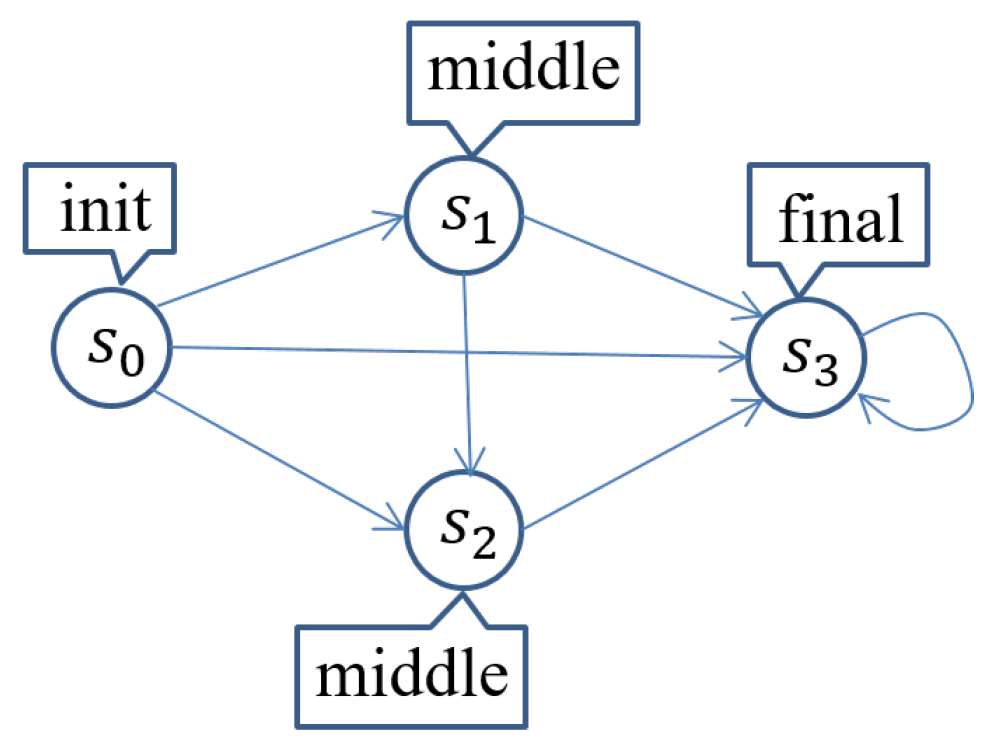
Let us outline the proposed technique with a simple system (or Kripke structure) called SimpSys as depicted in Figure 1 so that you can intuitively comprehend the technique. SimpSys has four states , , and , where is the only initial state. There are seven transitions depicted as arrows in Figure 1. Let us consider three atomic propositions , and . The labeling function is defined as depicted in Figure 1. For example, holds in and and does not in and . Let us take as a property concerned. We can straightforwardly check that SimpSys satisfies , namely , and then do not need to use the proposed technique for this model checking experiment. We, however, use this simple model checking experiment to sketch the technique.
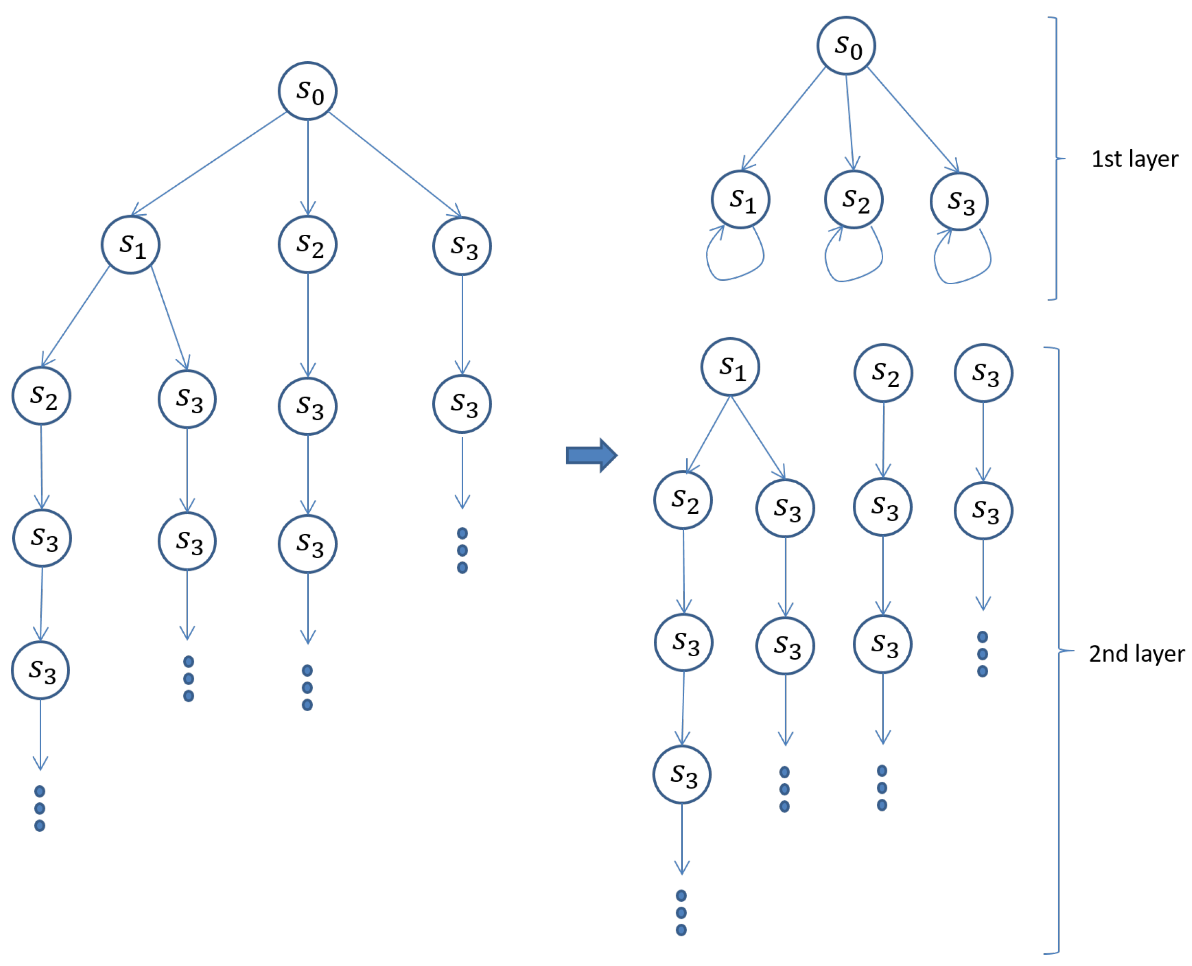
The left part of Figure 2 shows the computation tree made from the reachable states such that its root is the initial state . Let us split the computation tree into two layers such that the first layer depth is 1. Note that it is unnecessary to specify the second (or the final) layer depth. The first layer has one sub-state space such that its initial state is as shown in the right part of Figure 2. The second layer has three sub-state spaces such that their initial states are , and , respectively. We first conduct the model checking experiment that holds for the sub-state space in the first layer. There are two counterexamples: (1) and (2) , where and are called counterexample states. As holds for , we do not need to conduct the model checking experiment that holds for the sub-state space whose initial state is in the second layer. It suffices to conduct the model checking experiments that holds for the two sub-state spaces whose initial states are and , respectively. There are no counterexamples for the two model checking experiments and then we can conclude that SimpSys satisfies .
This is how the proposed technique works. For this simple example, the number of different states in each sub-state space is the same as or almost the same as the number of different states in the original state space. If the number of each sub-state space is much smaller than the number of the original state space, then even though it is impossible to conduct a model checking experiment for the original reachable state space because of the state space explosion, it may be possible to conduct the model checking experiment for each sub-state space. This is how the proposed technique mitigates the state space explosion problem.
4. Multiple Layer Division of Eventual Model Checking
This section describes the theoretical contribution of the paper. An overview of the proposed technique is as follows: an eventual model checking problem is divided into multiple smaller model checking problems and each smaller model checking problem is tackled so as to tackle the original eventual model checking experiment. We need to guarantee that tackling each smaller model checking problem is equivalent to tackling the original eventual model checking problem. We prove a theorem for it.
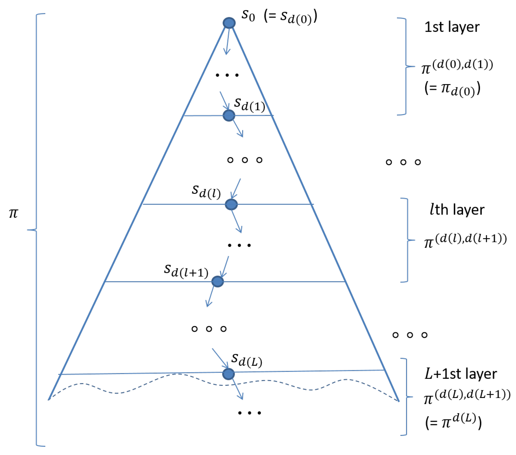
We prove that an eventual model checking problem for a Kripke structure and a path of is equivalent to eventual model checking problems for and paths of , where and the paths are obtained by splitting into parts. The paths are (), …, , …, (). Please see Figure 3.
We first tackle the case in which L is 1.
Lemma 1 (Two-layer division of ◊).
Let φ be any state proposition of . For any natural number k, . (We could use ∨ instead of ∨ because they are equivalent).
Proof.
(1) Case "only if" (⇒): There must be i such that . If , from Proposition 1 because φ is a state proposition. Thus, . Otherwise, . However, and . Hence, . (2) Case “if” (⇐): If , there must be i such that and . As φ is a state proposition, from Proposition 1 and then . If , then there must be j such that and . Thus, . □
Lemma 1 makes it possible to divide the original model checking problem into two model checking problems and . We only need to tackle unless holds.
Definition 5 ().
Let L be any non-zero natural number, k be any natural number and d be any function such that is 0, is a natural number for and is ∞.
- 1.
- 2.
Theorem 1 ( layer division of ◊).
Let L be any non-zero natural number. Let be 0, be any natural number for and be ∞. Let φ be any state proposition of . Then,
Proof.
By induction on L.
- Base case (): It follows from Lemma 1.
- Induction case (): We prove the following:Let be d used in such that , is an arbitrary natural number for and . The induction hypothesis is as follows:Let be d used in such that , is an arbitrary natural number for and . As is an arbitrary natural number for , we suppose that and for . As π is any path of , π can be replaced with . If so, we have the following as an instance of the induction hypothesis:From Definition 5, is because , and for and . Therefore, the induction hypothesis instance can be rephrased as follows:From Definition 5, iswhich isbecause of the induction hypothesis instance. From Lemma 1, this is equivalent to .
□
Theorem 1 makes it possible to divide the original model checking problem into model checking problems , …, , , …, . We only need to tackle if all of , …, do not hold.
5. A Divide and Conquer Approach to an Eventual Model Checking Algorithm
This section describes an algorithm that carries out the proposed technique. The algorithm takes as inputs a Kripke structure , a state proposition , a non-zero natural number L and a function d such that is a natural number for , where is the depth of layer x; and returns as an output success if holds and failure otherwise.
An algorithm can be constructed based on Theorem 1, which is shown as Algorithm 1. For each initial state , unfolding by using such that each node except for has exactly one incoming edge, an infinite tree whose root is is made. The infinite tree may have multiple copies of some states. Such an infinite tree can be divided into layers, as shown in Figure 3, where L is a non-zero natural number. Although there does not actually exist layer 0, it is convenient to just suppose that we have layer 0. Therefore, let us suppose that there is virtually layer 0 and is located at the bottom of layer 0. Let be the number of states located at the bottom of layer and then there are sub-state spaces in layer . In this way, the reachable state space from is divided into multiple smaller sub-state spaces. As is finite, the number of different states in each layer and in each sub-state space is finite. Theorem 1 makes it possible to check in a stratified way in that for each layer we can check for each , where is 0, is a non-zero natural number for and is ∞.
and are variables to which sets of states are set. Each iteration of the outermost loop in Algorithm 1, which conducts the model checking experiment in layer . , is the set of states located at the bottom of layer and is the empty set before the model checking experiments conducted in the st iteration. If for , then is added to . is set to at the end of each iteration. If is empty at the beginning of an iteration, is returned, meaning that holds. After the outermost loop, we check whether is empty. If so, is returned, and otherwise, is returned.
Although Algorithm 1 does not construct a counterexample when failure is returned, it could be constructed. For each , is prepared. As elements of , pairs are used, where s is a state in or a dummy state denoted that is different from any state in , is a state in and is reachable from s if . The assignment at line 6 should be revised as follows:
- ESl ← ∅
The assignment at line 10 should be revised as follows:
- ESl ← ESl ∪ {(s, π(d(l)))}
The assignment at line 14 should be revised as follows:
- ES ← {s | (s,s′) ∈ ESl}
is set to . We could then construct a counterexample, when failure is returned, by searching through , …, and .
| Algorithm 1: A divide and conquer approach to eventual model checking. |
 |
6. A Case Study
Many systems’ requirements can be expressed as eventual properties. Termination or halting is one important requirement that many programs should satisfy, which can be expressed as an eventual property. The starvation freedom property that should be satisfied by systems, such as an autonomous vehicle intersection control protocol [4], can be expressed as an eventual property. Some communication protocols, such as Alternating Bit Protocol (ABP) and the sliding window protocol used in Transmission Control Protocol (TCP), guarantee that all data sent by a sender are delivered to a receiver without any data loss and duplication. The requirement can be expressed as an eventual property.
We use a mutual exclusion protocol as an example in the case study. The requirement we take into account is that the protocol guarantees that a process can enter the critical section, doing some tasks there, leaving the section and reaching a final position (or terminating). The requirement can be expressed as an eventual property. The mutual exclusion protocol is called Qlock, an abstract version of the Dijkstra binary semaphore in that an atomic queue of process IDs is used.
In the rest of the section, we first describe Qlock, how to formally specify Qlock and the property concerned in Maude and how to model check the eventual property with the proposed technique. Let us note that when there are 10 processes that participate in Qlock, it is impossible to complete the model checking experiment with Maude LTL model checker, while it is possible to do so with the proposed technique. We finally summarize the case study.
6.1. Qlock
We report on a case study that demonstrates the power of the proposed technique. The case study used a mutual exclusion protocol called Qlock whose pseudo-code for each process p can be described as follows:
  “Start Section”
ss : enq(queue, p);
ws : repeat until top(queue) = p;
  “Critical Section”
cs : deq(queue);
fs : …
  “Finish Section”
where is an atomic queue of process IDs shared by all processes participating in Qlock. atomically puts a process ID p into at bottom. atomically returns the top element of . atomically deletes the top element of . If is empty, does nothing. is initially empty. Each process p is supposed to be located at one of the four locations (start section), (waiting section), (critical section) and (finish section), and is initially located at . Let us suppose that each process p stays once it gets there, implying that it enters the critical section at most once.
The property to be checked in this case study is that a process will eventually get to . The property can be formalized as an eventual property. When there were 10 processes, it did not complete the model check with the Maude LTL model checker running on a computer that carried a 2.10 GHz microprocessor and 8 GB main memory because of the state space explosion.
6.2. Formal Specification
We describe how to formally specify Qlock in Maude. A state is expressed as a braced soup of observable components, where observable components are name–value pairs and soups are associative–commutative collections. When there are n processes, the initial state of Qlock is as follows:
{(queue: empq) (pc[p1]: ss) … (pc[pn]: ss) (cnt: n)}
where (queue: empq) is an observable component saying that the shared queue is empty, (pc[pi]: ss) is an observable component saying that process pi is in the ss and (cnt: n) is an observable component whose value is a natural number n. The role of (cnt: n) will be described later.Transitions are described in terms of rewrite rules. The transitions of Qlock are specified as follows:
rl [start] : {(queue: Q) (pc[I]: ss) OCs} => {(queue: (Q | I)) (pc[I]: ws) OCs} .rl [wait] : {(queue: (I | Q)) (pc[I]: ws) OCs}
  => {(queue: (I | Q)) (pc[I]: cs) OCs} .
rl [exit] : {(queue: Q) (pc[I]: cs) (cnt: N) OCs}
  => {(queue: deq(Q)) (pc[I]: fs) (cnt: dec(N)) OCs} .
rl [fin] : {(cnt: 0) OCs} => {(cnt: 0) OCs} .
where Q is a variable of queues, I is a variable of process IDs, OCs is a variable of observable component soups and N is a variable of natural numbers. I | Q denotes a non-empty queue such that I is the top and Q is the remaining part of the queue. deq(Q) returns the empty queue if Q is empty and what is obtained by deleting the top from Q otherwise. dec(N) returns 0 if N is 0 and the predecessor number of N otherwise.start, wait, exit and fin are the labels given to the four rules, respectively. Rule start says that if process I is in ss, then it puts its ID into Q at end and moves to ws. Rule wait says that if process I is in ws and the top of the shared queue is I, then I enters cs. Rule exit says that if process I is in cs, then it deletes the top from the shared queue, decrements the natural number N stored in (cnt: N) and moves to fs. Rule fin says that if the natural number N stored in (cnt: N) is 0, a self-transition occurs. Rule fin is used to make the transitions total. The natural number N stored in (cnt: N) is the number of processes that have not yet reached fs. Use of it and rule fin make it unnecessary to use any fairness assumptions to model check an eventual property.
Let us consider one atomic proposition inFs1. inFs1 holds in a state if and only if the state matches {(pc[p1]: fs) OCs}, namely, that process p1 is in fs.
6.3. Model Checking with the Proposed Technique
It quickly completes to model check ◊ inFs1 for Qlock when there are five processes, finding no counterexample. It is, however, impossible to model check the same property for Qlock when there are 10 processes. We then use Algorithm 1 to tackle the latter case, where and .
We use one more observable component (depth: d), where d is a natural number, to work on the first layer. The initial state turns into the following:
{(queue: empq) (pc[p1]: ss) … (pc[p10)]: ss) (cnt: 10) (depth: 0)}The rules turn into the following:
crl [start] : {(queue: Q) (pc[I]: ss) (depth: D) OCs}
 => {(queue: (Q | I)) (pc[I]: ws) (depth: (D + 1)) OCs}
 if D < Bound .
crl [wait] : {(queue: (I | Q)) (pc[I]: ws) (depth: D) OCs}
 => {(queue: (I | Q)) (pc[I]: cs) (depth: (D + 1)) OCs}
 if D < Bound .
crl [exit] : {(queue: Q) (pc[I]: cs) (cnt: N)(depth: D) OCs}
 => {(queue: deq(Q)) (pc[I]: fs) (cnt: dec(N)) (depth: (D + 1)) OCs}
 if D < Bound .
crl [fin] : {(cnt: 0) (depth: D) OCs} => {(cnt: 0) (depth: (D + 1)) OCs}
 if D < Bound .
crl [stutter] :{(depth: D) OCs} => {(depth: D) OCs} if D >= Bound .
where D is a variable of natural numbers and Bound is 3. Rule stutter has been added to make each state at depth three have a transition to itself. The revised version of rule start says that if D is less than Bound and process I is in ss, then I puts its ID into Q at end and moves to ws and D is incremented. The other revised rules can be interpreted likewise. When we model checked ◊ inFs1 for the revised specification of Qlock, we found a counterexample that is a finite state sequence starting from the initial state and leading to a state loop that consists of one state that is as follows:
{(queue: (p1 | p2 | p3)) (cnt: 10) (depth: 3) (pc[p1]: ws)
 (pc[p2]: ws) (pc[p3]: ws) (pc[p4]: ss) (pc[p5]: ss) (pc[p6]: ss)
 (pc[p7]: ss) (pc[p8]: ss) (pc[p9]: ss) (pc[p10]: ss)}
We needed to find all counterexamples and then revise the definition of inFs1 such that inFs1 holds in the state as well. When we model checked the same property for the revised specification, we found another counterexample. This process was repeated until no more counterexamples were found. We totally found 819 counterexamples and 819 counterexample states at depth three.We gathered all states at depth three from the initial state, which totaled 820 states, including the 819 states found in the last step. There was one state at depth three such that process p1 was located at . For each of the 819 states as an initial state, we model checked ◊ inFs1 for the original specification of Qlock, finding no counterexample. Therefore, we can conclude that it completed model check ◊ inFs1 for Qlock when there were 10 processes, finding no counterexample. It took about 44 h to conduct the model checking experiments for the second layer and it took less than 200 ms to conduct each model checking experiment for the first layer. As there were 819 counterexamples for ◊ inFs1 in the first layer, we needed to conduct 820 model checking experiments for the first layer.
6.4. Summary of the Case Study
The proposed divide and conquer approach to eventual model checking makes it possible to successfully conduct the model checking experiment ◊ inFs1 for Qlock when there are 10 processes and each process enters the critical section at most once, which cannot be otherwise tackled by the computer used in the case study. The specifications in Maude used in the case study are available at the webpage (http://www.jaist.ac.jp/~ogata/code/dca2emc/).
7. Related Work
The state space explosion problem is one of the biggest challenges in model checking. Many techniques to mitigate it have been proposed so far. Among them are partial order reduction [12], symmetry reduction [13], abstraction [14,15,16], abstract logical model checking [17] and SAT-based bounded model checking (BMC) [2]. The proposed divide and conquer approach to eventual model checking is a new technique to mitigate the problem when model checking eventual properties. The second, third and fourth authors of the present paper proposed a (-layer) divide and conquer approach to leads-to model checking [18]. The technique proposed in the present paper can be regarded as an extension of the one described in the paper [18] to eventual properties.
Clarke et al. summarized several techniques that address the state space explosion problem in model checking [19]. One of them is SAT-based BMC. SAT-based BMC is used in industries, especially hardware industries. BMC can find a flaw located within some reasonably shallow depth k from each initial state but cannot prove that systems whose (reachable) state space is enormous (including infinite-state systems) enjoy the desired properties. Some extensions have been made to SAT-based BMC so that we can prove that such systems enjoy the desired properties. One extension is k-induction [20,21]. k-induction is a combination of mathematical induction and SAT/SMT-based BMC, where SMT stands for SAT modulo theories. The bounded state space from each initial state up to depth k is tackled with BMC, which is regarded as the base case. For each state sequence , where is an arbitrary state, such that a property concerned is not broken in each state for , it is checked that the property is not broken in all successor states of , which is done with an SAT/SMT solver and regarded as the induction case. If an SMT solver is used, infinite-state systems, for example, in which integers are used, could be handled. Our proposed technique can be regarded as another extension of BMC, although we do not use any SAT/SMT solvers.
SAT/SMT-based BMC has been extended to model check concurrent programs [22]. Given a concurrent (or multithreaded) program P together with two parameters u and r that are the loop unwinding bound and the number of round-robin schedules, respectively, an intermediate bounded program is first generated by unwinding all loops and inlining all function calls in P with u as a bound, except for those used for creating threads, and then is transformed into a sequential program that simulates all behaviors of within r round-robin schedules. is then transformed into a propositional formula, which is converted into an equisatisfiable CNF formula that can be analyzed by an SAT/SMT solver. This way to model check multithreaded programs can be parallelized by decomposing the set of execution traces of a concurrent program into symbolic subsets and analyzing the set of execution traces in parallel [23]. Instead of generating a single formula from P via , multiple propositional sub-formulas are generated. Each sub-formula corresponds to a different symbolic partition of the execution traces of P and can be checked for satisfiability independently from the others. The approaches to BMC of multithreaded programs seem able to deal with safety properties only, while our tool is able to deal with leads-to properties, a class of liveness properties. Another difference between their approach and our approach is that the target of our approach is designs of concurrent/distributed systems, while the one of theirs is concurrent programs.
Barnat et al. [24] surveyed some recent advancements of parallel model checking algorithms for LTL. Graph search algorithms need to be redesigned to make the best use of multi-core and/or multi-processor architectures. Parallel model checkers based on such parallel model checking algorithms have been developed, among which are DiVinE 3.0 [25], Garakabu2 [26,27] and a multicore extension of SPIN [28]. In the technique proposed in the present paper, there are generally multiple sub-state spaces in each layer, and model checking experiments for these sub-state spaces are totally independent from each other. Furthermore, model checking experiments for many sub-state spaces in different layers are independent. It is possible to conduct such model checking experiments in parallel. Therefore, it is possible to parallelize Algorithm 1, which never requires us to redesign any graph search algorithms and makes it possible to use any existing LTL model checker, such as Maude LTL model checker.
To tackle a large system that cannot be handled by an exhaustive verification mode, SPIN has a bit-state verification mode that may not exhaustively search the entire reachable state space of a large system, but can achieve a higher coverage of large state spaces by using a few bits of memory per state stored. The larger a system under verification becomes, the higher chances the SPIN bit-state verification mode may overlook flaws lurking in the system. To overcome such situations, swarm verification [29] has been proposed. The key ideas of swam verification are parallelism and search diversity. For each of the multiple different search strategies, one instance of bit-state verification is conducted. These instances are totally independent and can be conducted in parallel. Different search strategies traverse different portions of the entire reachable state space, making it more likely to achieve higher coverage of the entire reachable state space and find flaws lurking in a large system if any. An implementation of swarm verification on GPUs, called Grapple [30], has also been developed. Although the technique proposed in the present paper splits the reachable state space from each initial state into multiple layers, generating multiple sub-state spaces, it exhaustively searches each sub-state space with the Maude LTL model checker. It may be worth adopting the swarm verification idea into our technique such that swarm verification is conducted for each sub-state space instead of exhaustive search, which may make it possible to quickly find a flaw lurking in a large system.
One hot theme in research on methods to formally verify liveness properties including program termination is liveness-to-safety reductions. Biere et al. [31] have proposed a technique that formally verifies that finite-state systems satisfy liveness properties by showing the absence of fair cycles in every execution and coined the term “liveness-to-safety reduction” to refer to the technique. The technique can be extended to what is called “parameterized systems” in which the state space is infinite but actually finite for every system instance [32]. Padon et al. [33] have further extended “liveness-to-safety reduction” to systems such that processes can be dynamically created and each process state space is infinite so that they can formally verify that such systems enjoy liveness properties under fairness assumptions. Their technique basically reduces a infinite-state system liveness formal verification problem under fairness to a infinite-state system safety formal verification problem that can be expressed in first-order logic. The latter problem can be solved by existing first-order theorem provers, such as IC3 [34,35] and VAMPIRE [36]. The technique proposed in the present paper does not take into account fairness assumptions. We need to use fairness assumptions to model check liveness properties, including eventual ones from time to time. We might adopt the idea used in the Padon et al.’s liveness-to-safety reduction technique. To our knowledge, the liveness-to-safety reduction technique has not been parallelized. Our approach to eventual model checking might make it possible to parallelize the liveness-to-safety reduction technique.
8. Conclusions
We have proposed a new technique to mitigate the state explosion in model checking. The technique is dedicated to eventual properties. It divides an eventual model checking problem into multiple smaller model checking problems and tackles each smaller one. We have proved that the multiple smaller model checking problems are equivalent to the original eventual model checking problem. We have reported on a case study demonstrating the power of the proposed technique.
There are several things left to do as our future research. One piece of future work for us will be to develop a tool supporting the proposed technique. We will use Maude as an implementing language with its reflective programming (meta-programming) facilities to develop the tool that will do all necessary modifications to systems specifications (or systems models) so that human users do not need to change systems specifications to use the divide and conquer approach to eventual properties. It was impossible to conduct the model checking experiment with Maude LTL model checker; the autonomous vehicle intersection control protocol [4] enjoys the starvation freedom property when there are 13 vehicles with the tool supporting the proposed technique. The starvation freedom property can be expressed as an eventual property. Another piece of future work will be to complete the model checking experiment with the tool supporting the proposed technique. To complete the model checking experiment, we may need to make the best use of up-to-date multi-core/processor architectures. To this end, we need to parallelize Algorithm 1 and the tool supporting the proposed technique. Therefore, yet another piece of future work may be to evolve the tool into a parallel version that can make best use of up-to-date multi-core/processor architectures.
Author Contributions
Conceptualization, methodology, software, investigation and formal analysis, M.N.A., Y.P., C.M.D. and K.O.; project administration and funding acquisition, K.O. All authors have read and agreed to the published version of the manuscript.
Funding
This research was partially funded by JSPS KAKENHI Grant Number JP19H04082.
Institutional Review Board Statement
Not applicable.
Informed Consent Statement
Not applicable.
Data Availability Statement
The specifications in Maude used in the case study are available at the webpage http://www.jaist.ac.jp/~ogata/code/dca2emc/ (accessed on 16 January 2021).
Acknowledgments
The authors would like to thank the anonymous reviewers who carefully read an earlier version of the paper and gave them valuable comments without which they were not able to complete the present paper.
Conflicts of Interest
The authors declare no conflict of interest.
References
- Burch, J.R.; Clarke, E.M.; McMillan, K.L.; Dill, D.L.; Hwang, L.J. Symbolic Model Checking: 1020 States and Beyond. Inf. Comput. 1992, 98, 142–170. [Google Scholar] [CrossRef]
- Clarke, E.M.; Biere, A.; Raimi, R.; Zhu, Y. Bounded Model Checking Using Satisfiability Solving. Form. Methods Syst. Des. 2001, 19, 7–34. [Google Scholar] [CrossRef]
- Aung, M.N.; Phyo, Y.; Ogata, K. Formal Specification and Model Checking of the Lim-Jeong-Park-Lee Autonomous Vehicle Intersection Control Protocol. In Proceedings of the 31st International Conference on Software Engineering and Knowledge Engineering, SEKE 2019, Lisbon, Portugal, 10–12 July 2019; pp. 159–208. [Google Scholar] [CrossRef]
- Lim, J.; Jeong, Y.; Park, D.; Lee, H. An efficient distributed mutual exclusion algorithm for intersection traffic control. J. Supercomput. 2018, 74, 1090–1107. [Google Scholar] [CrossRef]
- Clavel, M.; Durán, F.; Eker, S.; Lincoln, P.; Martí-Oliet, N.; Meseguer, J.; Talcott, C. All About Maude—A High-Performance Logical Framework: How to Specify, Program and Verify Systems in Rewriting Logic; Lecture Notes in Computer Science (LNCS); Springer: Berlin/Heidelberg, Germany, 2007; Volume 4350. [Google Scholar] [CrossRef]
- Holzmann, G.J. The SPIN Model Checker—Primer and Reference Manual; Addison-Wesley: Reading, MA, USA, 2004. [Google Scholar]
- Goguen, J.A.; Kirchner, C.; Kirchner, H.; Mégrelis, A.; Meseguer, J.; Winkler, T.C. An Introduction to OBJ 3. In Proceedings of the Conditional Term Rewriting Systems, 1st International Workshop, Orsay, France, 8–10 July 1987; Lecture Notes in Computer Science; Kaplan, S., Jouannaud, J., Eds.; Springer: Berlin/Heidelberg, Germany, 1987; Volume 308, pp. 258–263. [Google Scholar] [CrossRef]
- Diaconescu, R.; Futatsugi, K. Cafeobj Report—The Language, Proof Techniques, and Methodologies for Object-Oriented Algebraic Specification; AMAST Series in Computing; World Scientific: Singapore, 1998; Volume 6. [Google Scholar] [CrossRef]
- Cimatti, A.; Clarke, E.M.; Giunchiglia, E.; Giunchiglia, F.; Pistore, M.; Roveri, M.; Sebastiani, R.; Tacchella, A. NuSMV 2: An OpenSource Tool for Symbolic Model Checking. In Proceedings of the Computer Aided Verification, 14th International Conference, CAV 2002, Copenhagen, Denmark, 27–31 July 2002; Lecture Notes in Computer Science; Brinksma, E., Larsen, K.G., Eds.; Springer: Berlin/Heidelberg, Germany, 2002; Volume 2404, pp. 359–364. [Google Scholar] [CrossRef]
- Ogata, K.; Futatsugi, K. Comparison of Maude and SAL by Conducting Case Studies Model Checking a Distributed Algorithm. IEICE Trans. Fundam. Electron. Commun. Comput. Sci. 2007, 90, 1690–1703. [Google Scholar] [CrossRef]
- de Moura, L.M.; Owre, S.; Rueß, H.; Rushby, J.M.; Shankar, N.; Sorea, M.; Tiwari, A. SAL 2. Computer Aided Verification. In Proceedings of the 16th International Conference, CAV 2004, Boston, MA, USA, 13–17 July 2004; Lecture Notes in Computer Science; Alur, R., Peled, D.A., Eds.; Springer: Berlin/Heidelberg, Germany, 2004; Volume 3114, pp. 496–500. [Google Scholar] [CrossRef]
- Clarke, E.M.; Grumberg, O.; Minea, M.; Peled, D.A. State Space Reduction Using Partial Order Techniques. Int. J. Softw. Tools Technol. Transf. 1999, 2, 279–287. [Google Scholar] [CrossRef]
- Clarke, E.M.; Emerson, E.A.; Jha, S.; Sistla, A.P. Symmetry Reductions in Model Checking. In Proceedings of the CAV 1998, Vancouver, BC, Canada, 28 June–2 July 1998; Lecture Notes in Computer Science; Springer: Vancouver, BC, Canada, 1998; Volume 1427, pp. 147–158. [Google Scholar] [CrossRef]
- Clarke, E.M.; Grumberg, O.; Long, D.E. Model Checking and Abstraction. ACM Trans. Program. Lang. Syst. 1994, 16, 1512–1542. [Google Scholar] [CrossRef]
- Clarke, E.M.; Grumberg, O.; Jha, S.; Lu, Y.; Veith, H. Counterexample-guided abstraction refinement for symbolic model checking. J. ACM 2003, 50, 752–794. [Google Scholar] [CrossRef]
- Meseguer, J.; Palomino, M.; Martí-Oliet, N. Equational abstractions. Theor. Comput. Sci. 2008, 403, 239–264. [Google Scholar] [CrossRef]
- Bae, K.; Escobar, S.; Meseguer, J. Abstract Logical Model Checking of Infinite-State Systems Using Narrowing. In Proceedings of the RTA 2013, Eindhoven, The Netherlands, 24–26 June 2013; LIPIcs; Schloss Dagstuhl–Leibniz-Zentrum fuer Informatik: Eindhoven, The Netherlands, 2013; Volume 21, pp. 81–96. [Google Scholar] [CrossRef]
- Phyo, Y.; Minh, C.D.; Ogata, K. A Divideeventual model checking Conquer Approach to Leads-to Model Checking. Comput. J. 2021. [Google Scholar] [CrossRef]
- Clarke, E.M.; Klieber, W.; Novácek, M.; Zuliani, P. Model Checking and the State Explosion Problem. In LASER Summer School 2011; Lecture Notes in Computer Science; Springer: Elba Island, Italy, 2011; Volume 7682, pp. 1–30. [Google Scholar] [CrossRef]
- Sheeran, M.; Singh, S.; Stålmarck, G. Checking Safety Properties Using Induction and a SAT-Solver. In Proceedings of the FMCAD, Austin, TX, USA, 1–3 November 2000; Lecture Notes in Computer Science; Springer: Austin, TX, USA, 2000; Volume 1954, pp. 108–125. [Google Scholar] [CrossRef]
- de Moura, L.M.; Rueß, H.; Sorea, M. Bounded Model Checking and Induction: From Refutation to Verification. In Proceedings of the CAV 2003, Boulder, CO, USA, 8–12 July 2003; Lecture Notes in Computer Science; Springer: Boulder, CO, USA, 2003; Volume 2725, pp. 14–26. [Google Scholar] [CrossRef]
- Inverso, O.; Tomasco, E.; Fischer, B.; Torre, S.L.; Parlato, G. Bounded Model Checking of Multi-threaded C Programs via Lazy Sequentialization. In Proceedings of the Computer Aided Verification—26th International Conference, CAV 2014, Held as Part of the Vienna Summer of Logic, VSL 2014, Vienna, Austria, 18–22 July 2014; Lecture Notes in Computer Science; Biere, A., Bloem, R., Eds.; Springer: Berlin/Heidelberg, Germany, 2014; Volume 8559, pp. 585–602. [Google Scholar] [CrossRef]
- Inverso, O.; Trubiani, C. Parallel and distributed bounded model checking of multi-threaded programs. In Proceedings of the PPoPP ’20: 25th ACM SIGPLAN Symposium on Principles and Practice of Parallel Programming, San Diego, CA, USA, 22–26 February 2020; Gupta, R., Shen, X., Eds.; ACM: New York, NY, USA, 2020; pp. 202–216. [Google Scholar] [CrossRef]
- Barnat, J.; Bloemen, V.; Duret-Lutz, A.; Laarman, A.; Petrucci, L.; van de Pol, J.; Renault, E. Parallel Model Checking Algorithms for Linear-Time Temporal Logic. In Handbook of Parallel Constraint Reasoning; Springer: Berlin/Heidelberg, Germany, 2018; pp. 457–507. [Google Scholar] [CrossRef]
- Barnat, J.; Brim, L.; Havel, V.; Havlícek, J.; Kriho, J.; Lenco, M.; Rockai, P.; Still, V.; Weiser, J. DiVinE 3.0—An Explicit-State Model Checker for Multithreaded C & C++ Programs. In CAV 2013; LNCS; Springer: Berlin/Heidelberg, Germany, 2013; Volume 8044, pp. 863–868. [Google Scholar] [CrossRef]
- Kong, W.; Liu, L.; Ando, T.; Yatsu, H.; Hisazumi, K.; Fukuda, A. Facilitating Multicore Bounded Model Checking with Stateless Explicit-State Exploration. Comput. J. 2015, 58, 2824–2840. [Google Scholar] [CrossRef]
- Kong, W.; Hou, G.; Hu, X.; Ando, T.; Hisazumi, K.; Fukuda, A. Garakabu2: An SMT-based bounded model checker for HSTM designs in ZIPC. J. Inf. Sec. Appl. 2016, 31, 61–74. [Google Scholar] [CrossRef]
- Holzmann, G.J.; Bosnacki, D. The Design of a Multicore Extension of the SPIN Model Checker. IEEE Trans. Softw. Eng. 2007, 33, 659–674. [Google Scholar] [CrossRef]
- Holzmann, G.J.; Joshi, R.; Groce, A. Swarm Verification Techniques. IEEE Trans. Softw. Eng. 2011, 37, 845–857. [Google Scholar] [CrossRef]
- DeFrancisco, R.; Cho, S.; Ferdman, M.; Smolka, S.A. Swarm model checking on the GPU. Int. J. Softw. Tools Technol. Transf. 2020, 22, 583–599. [Google Scholar] [CrossRef]
- Biere, A.; Artho, C.; Schuppan, V. Liveness Checking as Safety Checking. Electron. Notes Theor. Comput. Sci. 2002, 66, 160–177. [Google Scholar] [CrossRef]
- Pnueli, A.; Shahar, E. Liveness and Acceleration in Parameterized Verification. In Proceedings of the Computer Aided Verification, 12th International Conference, CAV 2000, Chicago, IL, USA, 15–19 July 2000; Lecture Notes in Computer Science; Emerson, E.A., Sistla, A.P., Eds.; Springer: Berlin/Heidelberg, Germany, 2000; Volume 1855, pp. 328–343. [Google Scholar] [CrossRef]
- Padon, O.; Hoenicke, J.; Losa, G.; Podelski, A.; Sagiv, M.; Shoham, S. Reducing liveness to safety in first-order logic. Proc. ACM Program. Lang. 2018, 2, 1–33. [Google Scholar] [CrossRef]
- Bradley, A.R. Understanding IC3. In Proceedings of the Theory and Applications of Satisfiability Testing—SAT 2012—15th International Conference, Trento, Italy, 17–20 June 2012; Lecture Notes in Computer Science; Cimatti, A., Sebastiani, R., Eds.; Springer: Berlin/Heidelberg, Germany, 2012; Volume 7317, pp. 1–14. [Google Scholar] [CrossRef]
- Bradley, A.R. IC3 and beyond: Incremental, Inductive Verification. In Proceedings of the Computer Aided Verification—24th International Conference, CAV 2012, Berkeley, CA, USA, 7–13 July 2012; Lecture Notes in Computer Science; Madhusudan, P., Seshia, S.A., Eds.; Springer: Berlin/Heidelberg, Germany, 2012; Volume 7358, p. 4. [Google Scholar] [CrossRef]
- Riazanov, A.; Voronkov, A. The design and implementation of VAMPIRE. AI Commun. 2002, 15, 91–110. [Google Scholar]
Figure 1.
A simple system called SimpSys.

Figure 2.
Two-layer division of the SimpSys reachable state space.

Figure 3.
layer division of the reachable state space.


Table 1.
Descriptions of path notations (or symbols), where i and j are natural numbers.
| Symbol | Description |
|---|---|
| a path; an infinite sequence of states such that for each i; | |
| if is an initial state, it is called a computation | |
| the ith state in | |
| the postfix obtained by deleting the first i states from | |
| constructed by first extracting the prefix , the first states from | |
| and then adding , the final state of the prefix, to the prefix at the end infinitely many times | |
| , the same as | |
| if , then , the same as ; | |
| otherwise, , the infinite sequence in which only occurs infinitely many times | |
| , the same as | |
| the same as |
Table 2.
Descriptions of path-set notations (or symbols), where b is a natural number.
| Symbol | Description |
|---|---|
| the set of all paths of | |
| the set of all paths of such that , the 0th state of the path , is s | |
| the set of all paths such that | |
| the same as |
Table 3.
Descriptions of satisfaction relation ⊧ notations (or symbols), where b is a natural number.
Table 3.
Descriptions of satisfaction relation ⊧ notations (or symbols), where b is a natural number.
| Symbol | Description |
|---|---|
| an LTL formula holds for a path of | |
| an LTL formula holds for all computations of | |
| an LTL formula holds for all paths in | |
| an LTL formula holds for all paths in | |
| the same as |
Publisher’s Note: MDPI stays neutral with regard to jurisdictional claims in published maps and institutional affiliations. |
© 2021 by the authors. Licensee MDPI, Basel, Switzerland. This article is an open access article distributed under the terms and conditions of the Creative Commons Attribution (CC BY) license (http://creativecommons.org/licenses/by/4.0/).
Share and Cite
MDPI and ACS Style
Aung, M.N.; Phyo, Y.; Do, C.M.; Ogata, K. A Divide and Conquer Approach to Eventual Model Checking. Mathematics 2021, 9, 368. https://0-doi-org.brum.beds.ac.uk/10.3390/math9040368
AMA Style
Aung MN, Phyo Y, Do CM, Ogata K. A Divide and Conquer Approach to Eventual Model Checking. Mathematics. 2021; 9(4):368. https://0-doi-org.brum.beds.ac.uk/10.3390/math9040368
Chicago/Turabian StyleAung, Moe Nandi, Yati Phyo, Canh Minh Do, and Kazuhiro Ogata. 2021. "A Divide and Conquer Approach to Eventual Model Checking" Mathematics 9, no. 4: 368. https://0-doi-org.brum.beds.ac.uk/10.3390/math9040368
Note that from the first issue of 2016, this journal uses article numbers instead of page numbers. See further details here.