An Econometric Approach Regarding the Impact of Fiscal Pressure on Equilibrium: Evidence from Electricity, Gas and Oil Companies Listed on the New York Stock Exchange

Abstract

The matter of fiscal pressure is more current than ever in most countries around the world for various reasons. In the first place, disruptive phenomena such as financial crises put tremendous pressure on worldwide economies. Secondly, high taxes trigger an overall reduction in the level of investments aiming at creating stable and well-paid jobs. Thirdly, the income generated by the majority of taxpayers is subject to excessive taxation, which may fuel tax evasion acts. On these grounds, the article is the first empirical research investigating the impact of fiscal pressure on the financial equilibrium of energy companies listed on the New York Stock Exchange. The sample included 88 electricity, gas, and oil companies from around the world, which were analyzed over a time span of 16 years, including the periods before, during, and after the 2008 global financial crisis. The methodology entailed estimating econometric models via Panel Least Squares (cross-section weights) with and without time fixed effects. Empirical results showed that fiscal pressure had a stronger impact on the short-term and long-term equilibrium of electricity and oil companies than on the equilibrium of gas companies. The study can serve as a compass for the managers of energy companies interested in estimating the evolution of company equilibrium state when considering other potential financial downturns.

1. Introduction

Exploring the impact of fiscal pressure is a timely topic especially because of the excessively increasing national debt levels during the last decade, after the 2008 global financial crisis [1,2,3]. The effects of such an increase have been negatively perceived on international financial markets by both individual and corporate taxpayers. In addition, high levels of fiscal pressure generally discourage individual taxpayers from saving, investing, or even working. High levels of fiscal pressure can also discourage corporate taxpayers from investing into new production capacities [4], hiring staff from the people available on the labor market, increasing production levels, and contributing to public budgets. Moreover, in recent years, tax systems from developed countries have undergone significant reforms as a result of investors’ reactions on international markets. For that matter, the 2008 global financial crisis, the intricacy of tax behavior scrutinized by various economic and behavioral models [5], the complexity of tax systems across different countries and the negative externalities posed by phenomena such as shadow economy and corruption [6], the dynamics of the relationship between tax authorities and taxpayers [7], and the impact of taxes on economic growth are important factors that have contributed to the implementation of the aforementioned tax reforms.

Going back to the core of the anomalous national debt levels, it is noteworthy to state that, in recent history, the 2008 global financial crisis was a major financial meltdown that has disclosed once more the fragility and the interconnectedness of global economies in general and of stock markets in particular. Nearly all industries across world economies were negatively shaped by the global crisis and the energy industry (e.g., electricity, gas, oil suppliers) was no exception to the rule in this equation. On the account of the crisis, companies providing energy services (especially those publicly traded) have faced challenges in terms on demand, financing, and expansion [8,9,10,11], which lasted for several years.

The present research study focused on integrants from the energy industry due to the crucial role these companies play for both economic activities and overall human societies. For that matter, corporate and individual taxpayers rely on energy supplied by electricity, gas, and oil companies for their day-to-day operations and lives. Moreover, price fluctuations on the energy market are usually mirrored by price fluctuations of all categories of goods and services, since their production, distribution, sale, and consumption is organically linked to the energy industry.

For the purpose of this study, the sample comprised 88 electricity, gas, and oil companies from various countries around the world (e.g., Argentina, Austria, Brazil, Canada, France, Germany, Ireland, Italy, Norway, Portugal, Russia, South Korea, Spain, USA), most of companies operating on multiple international markets. The time span of 2005Q1–2020Q3 was selected in order to allow for the incorporation of the period before, during, and after the 2008 global financial crisis. Considering that this financial cataclysm was the second major downturn affecting stock markets following the 1929 Great Depression, the choice of the time frame seemed propitious.

Within the market economy, the development of any company is unquestionably related to ensuring its economic equilibrium. In this sense, financial equilibrium indicates the equality and relationships between the necessary financial resources and the possibilities of collecting these resources. The financial equilibrium of a company requires covering various expenses: all operating expenses from company income or loans; all expenses that are not included in costs; costs of company development and modernization; expenses to incentivize staff and shareholders; contractual obligations and financial commitments toward banks and the state budget.

Financial equilibrium is measured through the states of liquidity and solvency. Liquidity is a state of financial equilibrium expressing the company’s ability of meeting short-term payments by synchronizing cash inflows and outflows during the fiscal year. Solvency is the company’s ability of meeting long-term payments. The state of liquidity depends on the company operating cycle, namely the time between the purchase of raw materials and the conversion of finished goods into cash or an instrument easily convertible into cash. The state of solvency is specific to the financial cycle comprising three overlapping cycles: operational cycle, investment cycle, and financing cycle.

The first goal of the article consists in identifying to what extent liquidity can be influenced by fiscal pressure—measured through ratios such as fiscal pressure to expenses, fiscal pressure to equity, fiscal pressure to gross margin, and fiscal pressure to sales—because such information brings interesting insights when analyzing short-term equilibrium based on accounting data. The second goal is the investigation of the degree to which fiscal pressure influences company solvency.

The novelty of the article resides in the fact that, to the best of my knowledge, this is first empirical research focused on the link between fiscal pressure and financial equilibrium for energy companies listed on the stock exchange market. Economic theory stipulates that, despite an increase in fiscal pressure, the state of equilibrium remains constant. The article shows that short and long-term equilibria were influenced by fiscal pressure in the case of electricity, gas, and oil companies. According to empirical results, fiscal pressure had a stronger impact on the short-term and long-term equilibrium of electricity and oil companies than on the equilibrium of gas companies.

The article has the following structure. Section 2 named Literature Review highlights relevant recent studies investigating the topic of fiscal pressure. Section 3 labelled Materials and Methods describes the company sample and the variables of interest. Section 4 named Results presents the hypotheses, proposed econometric models, and estimated outcomes. Section 5 discusses the main results, while Section 6 includes limitations and future research directions, while drawing conclusions.

2. Literature Review

According to public finance theory, the most important role of tax revenues (direct and indirect taxes, social contributions levied on labor, fiscal fees for various services provided by public authorities) resides in their support of public budgets used by state authorities to finance public outlays [12,13]. In the absence of effective taxation instruments and streamlined tax systems lacking excessive red tape, public goods entailing air quality, cultural goods, education, healthcare, social security, national defense, rule of law, transport infrastructure, etc., would cease to exist.

Given the fact that, in the majority of countries, tax revenues are levied in reference to income, wealth, consumption, or labor via different tax rates (either flat or progressive), they trigger the so-called fiscal pressure on corporate [14,15] and individual taxpayers. Moreover, because of the tendency of certain countries in the Middle East to gradually mitigate dependence on natural resource revenues, fiscal pressure has increased even more on their taxpayers following the enactment of the value added tax (VAT), which until recently was known to these taxpayers only in theory [16].

Various studies in the extant literature illustrate empirical results concerning the fiscal pressure exerted by taxation on taxpayers, communities, countries, and regions [17,18,19,20]. Nevertheless, there are no particular studies investigating the impact of fiscal pressure on the short and long-term financial equilibrium of publicly traded companies from the energy industry. Therefore, the present study aims to close the gap in the literature by focusing on this particular research direction.

As a case in point, using data from 40 European countries investigated during eleven years, Molina-Morales et al. [21] analyzed various factors shaping fiscal pressure, including economic freedom of Eurozone members and the ideology of the ruling party. Results showed that Eurozone members, countries ruled by left-wing parties, and countries that were former members of the Soviet bloc were more likely to exhibit a higher fiscal pressure on their citizens.

Villar Rubio et al. [22] investigated the convergence regarding environmental fiscal pressure by taking into account economic globalization and fiscal harmonization. The country sample included the first 15 members of the European Union and the authors applied beta, sigma, and gamma convergence tools to the data retrieved from Eurostat for the period 1987–2008. Results indicated the existence of convergence with respect to environmental tax pressure in all countries, except for Denmark and the Netherlands, which already registered high levels of environmental tax pressure.

Trussel and Patrick [23] studied whether fiscal pressure was positively linked to income concentration and debt utilization and whether it was negatively linked to organizational weakness and entity resources. Results indicated that fiscal pressure was mostly connected with a low level of capital expenditures concerning overall budget revenues and revenues from bonds issued by governmental authorities.

Ezeoha and Ogamba [24] analyzed the influence of taxation on managerial decisions and observed that taxes impacted on the level and structure of funding sources within a company. On the one hand, dividend policy was a strategic function of financial management and was influenced by dividend tax and capital gains tax. On the other hand, the company debt level was conditioned by the access to markets for long-term financing. Therefore, the authors emphasized the major role played by company solvency for obtaining financial support from the market.

In a study conducted on 100 bankrupt and non-bankrupt small, medium, and large Croatian companies, Bubić, Mladineo, and Šušak [25] studied the degree to which changes in the VAT rate would influence company liquidity. Empirical results estimated on financial data before and after the VAT rate change (i.e., from 22% in 2008 to 23% in 2010) showed that liquidity proxied via cash ratio was significantly affected in the case of bankrupt companies. At the other end of the spectrum, companies not facing insolvency did not register any changes in their liquidity levels after the fiscal policy changes had been enacted.

3. Materials and Methods

In this research study, I estimated the relationships between fiscal pressure indicators (i.e., fiscal pressure to gross margin, fiscal pressure to equity, fiscal pressure to sales, fiscal pressure to expenses) and indicators reflecting the state of equilibrium of a company (i.e., current ratio, quick ratio, debt to equity ratio) on the short and long run of companies operating in the energy industry.

Indicators were chosen to provide a more in-depth analysis of the company state based on strong econometric estimations of the aforementioned relationships. To go beyond mere descriptive accounts portraying the company state at a particular moment in time, the sample included data from 88 electricity, gas, and oil companies listed on the New York Stock Exchange, whose evolution was tracked over a period of almost 16 years (2005Q1–2020Q3).

The company sample was compiled based on the following rationale. In a first step, the focus was on identifying companies publicly traded on the New York Stock Exchange and operating in the electricity, gas, and oil sectors because these are the fundamental sectors within energy industry. In a second step, companies were selected among worldwide suppliers of energy in the descending order of their market capitalization. In a third step, only companies with complete financial reporting were considered. The final sample included the 88 companies headquartered in various countries around the world (see Appendix A for company details).

The outcome variables considered for the empirical analyses were the following:

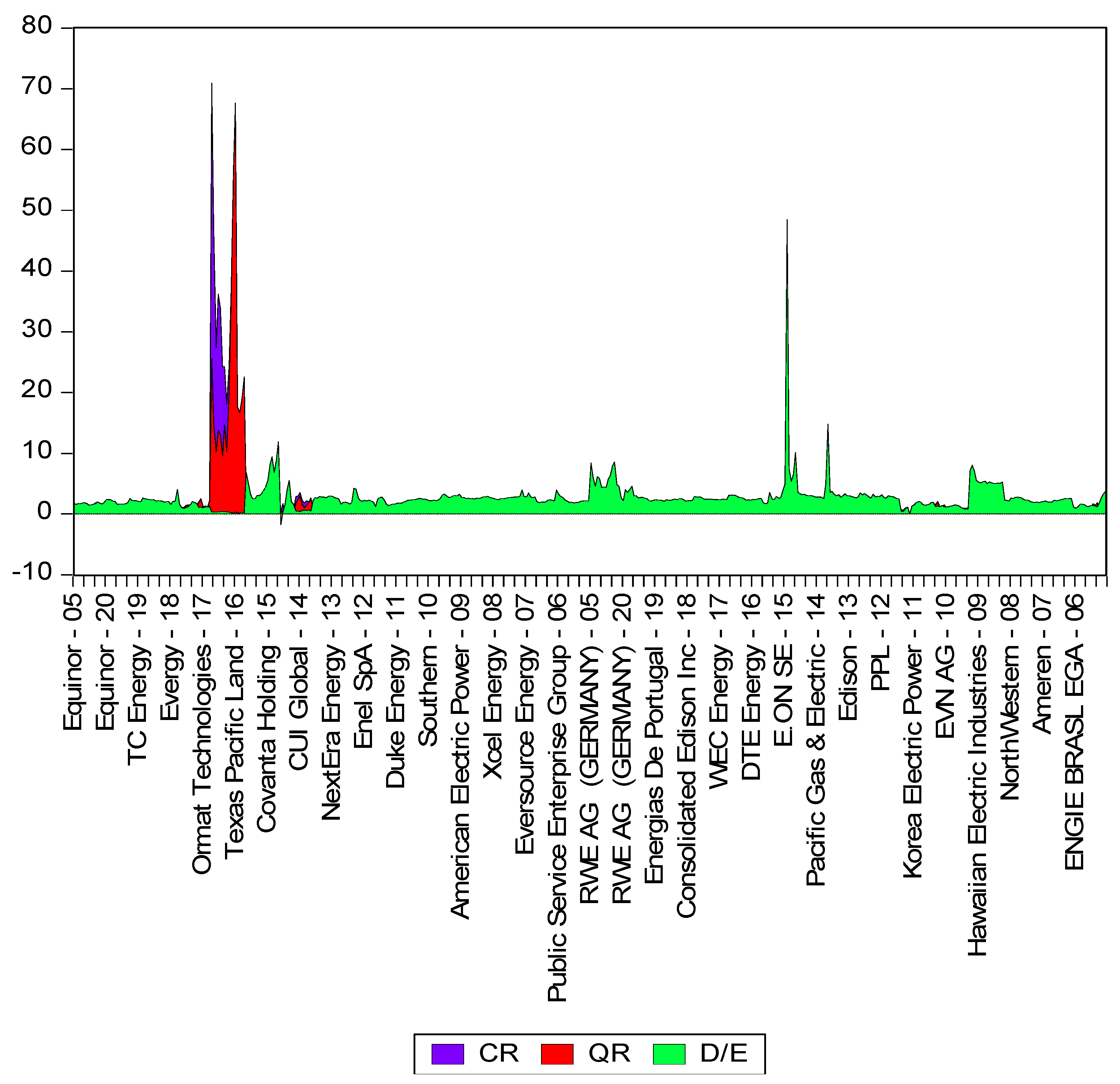
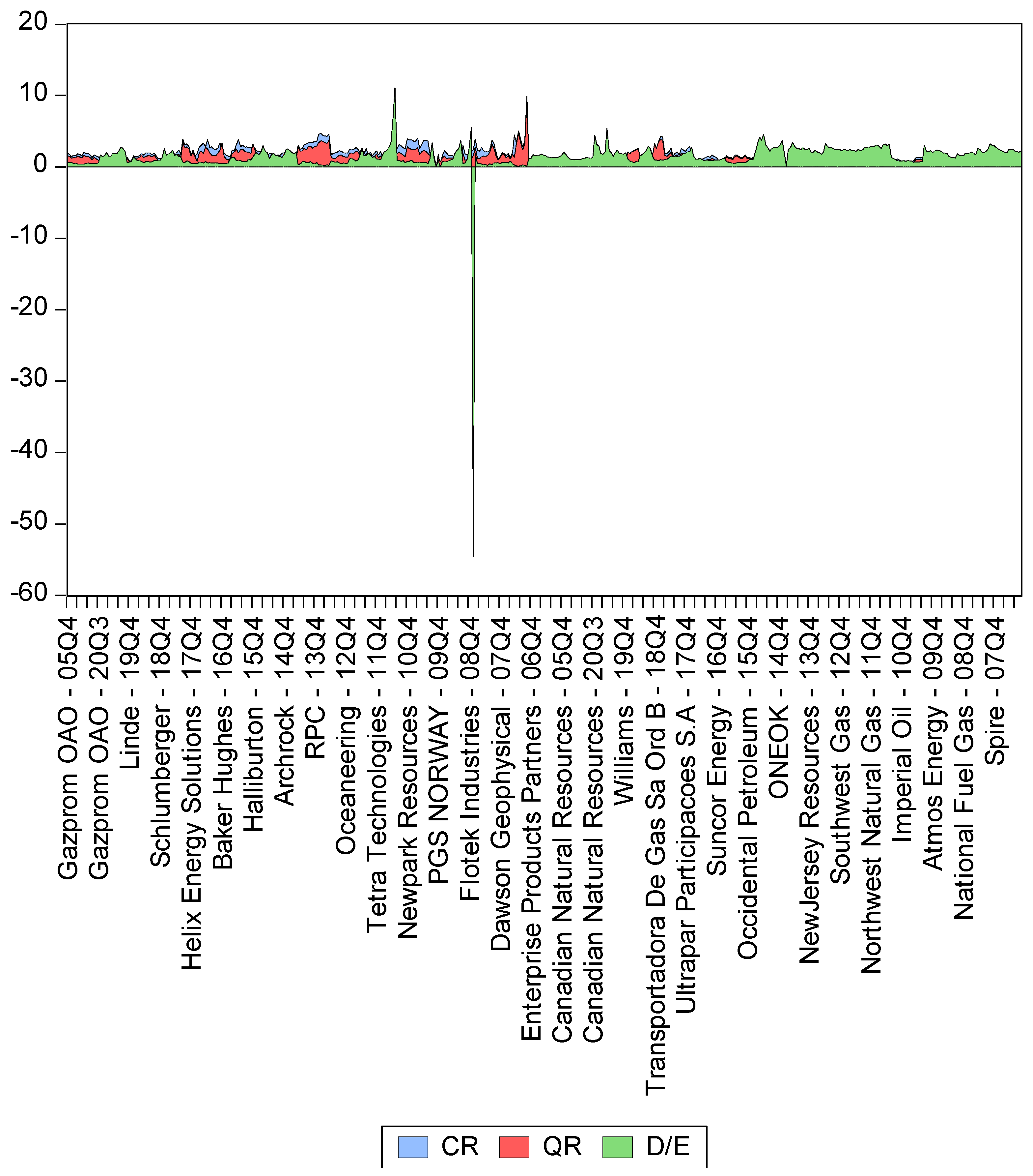
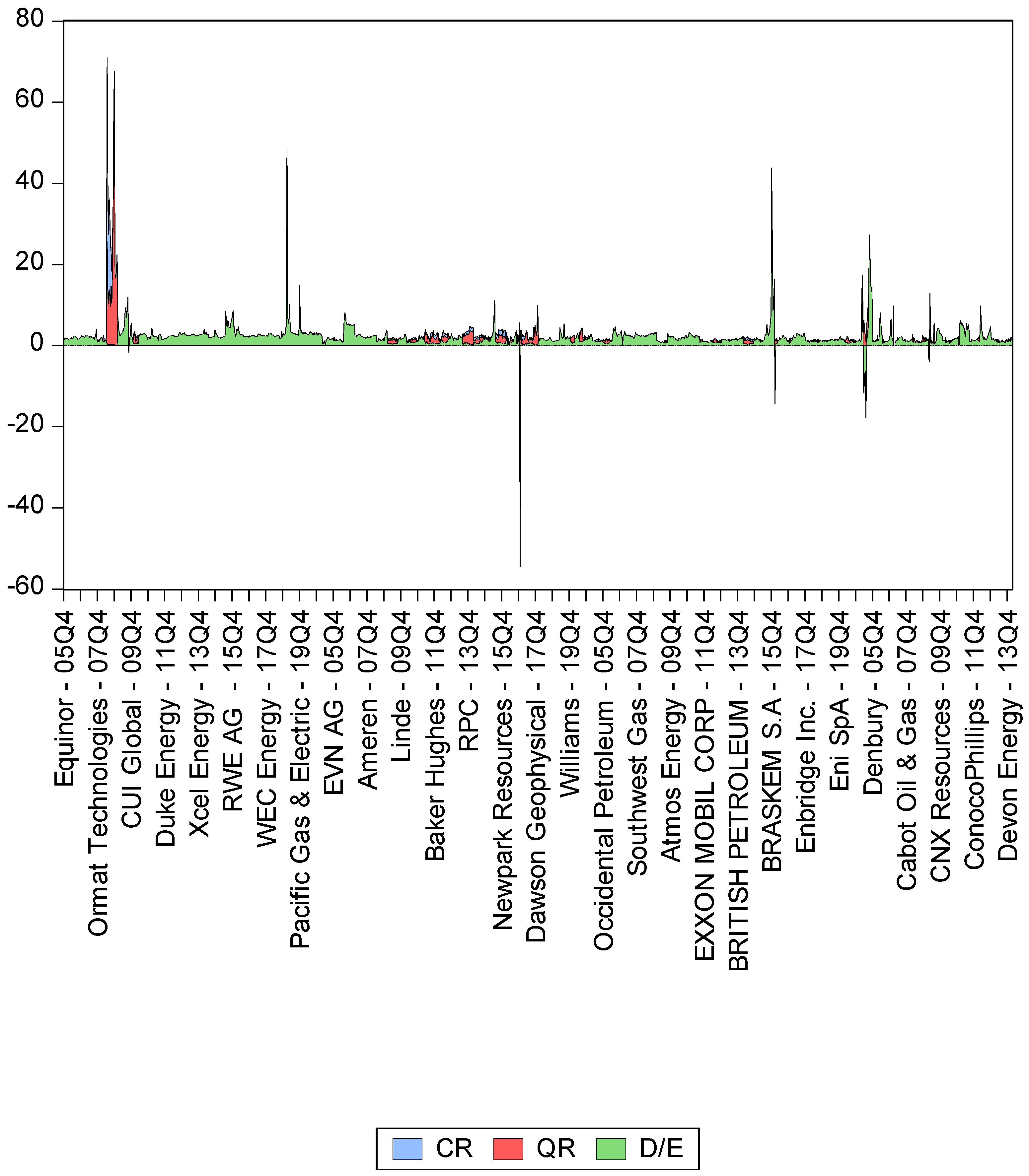
• Current liquidity ratio (CR), which reflects the capacity of current assets (e.g., inventory, short-term investments) to turn into cash that should cover the outstanding debts of the company. According to financial analysts, a company has a favorable liquidity when the current ratio ranges from 150% to 250% (generally);
• Quick ratio (QR), determined as a ratio between more liquid current assets (receivables, short-term investments) and current liabilities. A favorable quick ratio should range between 50% and 100% (generally);
• Debt to equity ratio (D/E), expressing the ability of a company to cope with external payments, is calculated by dividing debt to equity. The optimum value of the indicator is 0–30% (the so-called “green area”). The range 31–50% is called the “brown area,” 51–70% is the “red area,” while everything above 70% belongs to the “black area.”

The explanatory variables considered for the empirical analyses were the following:

4.

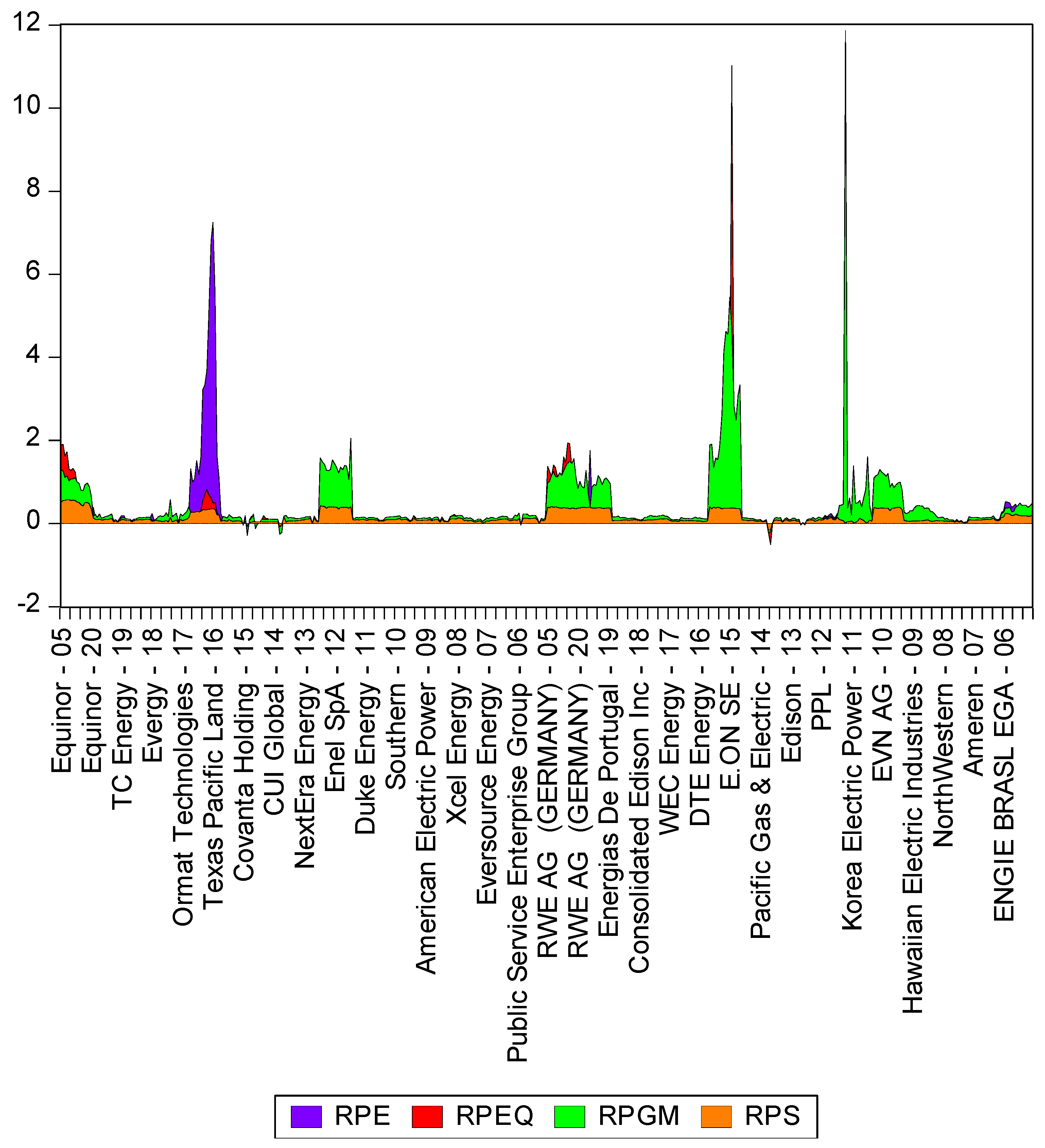
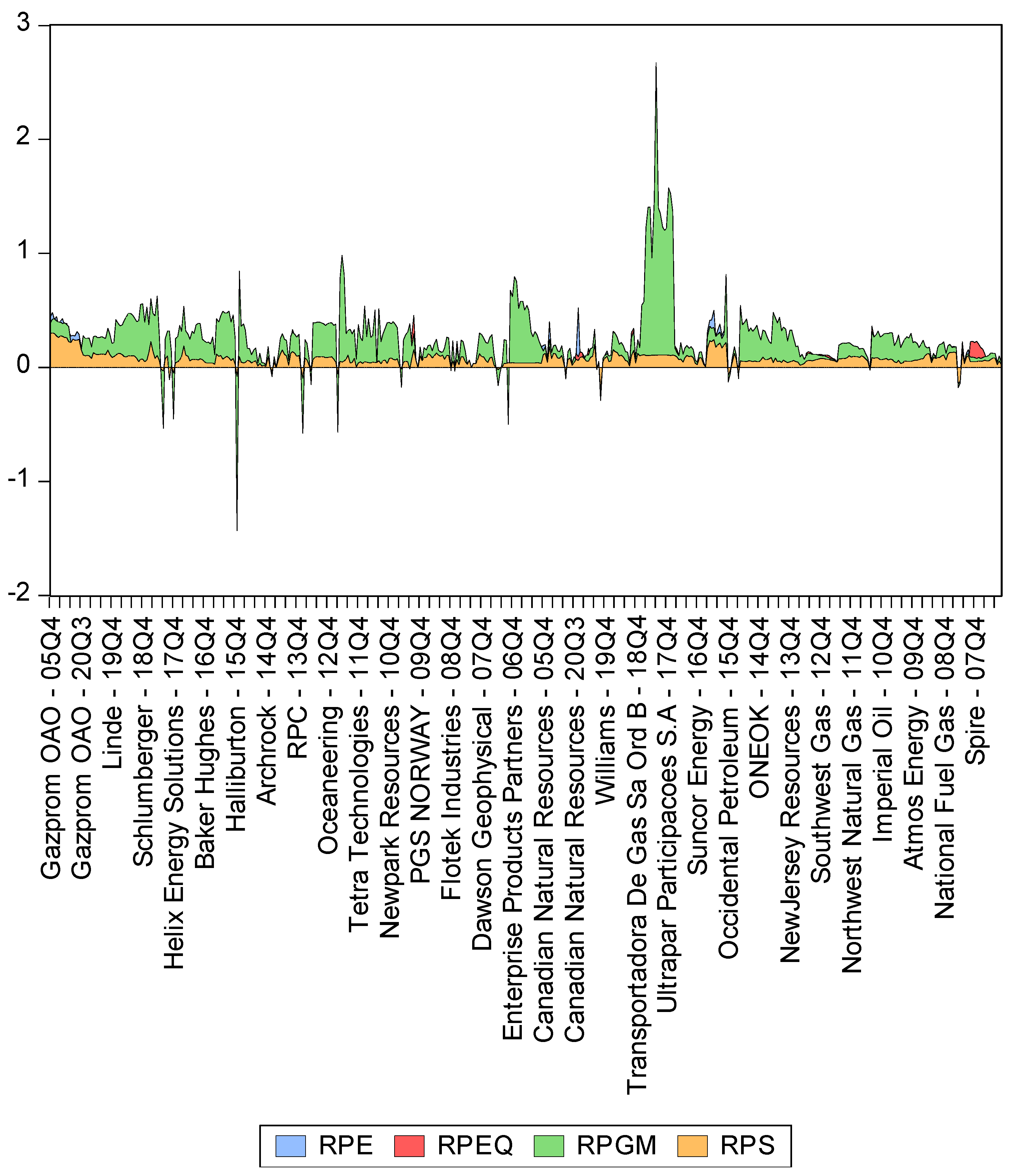
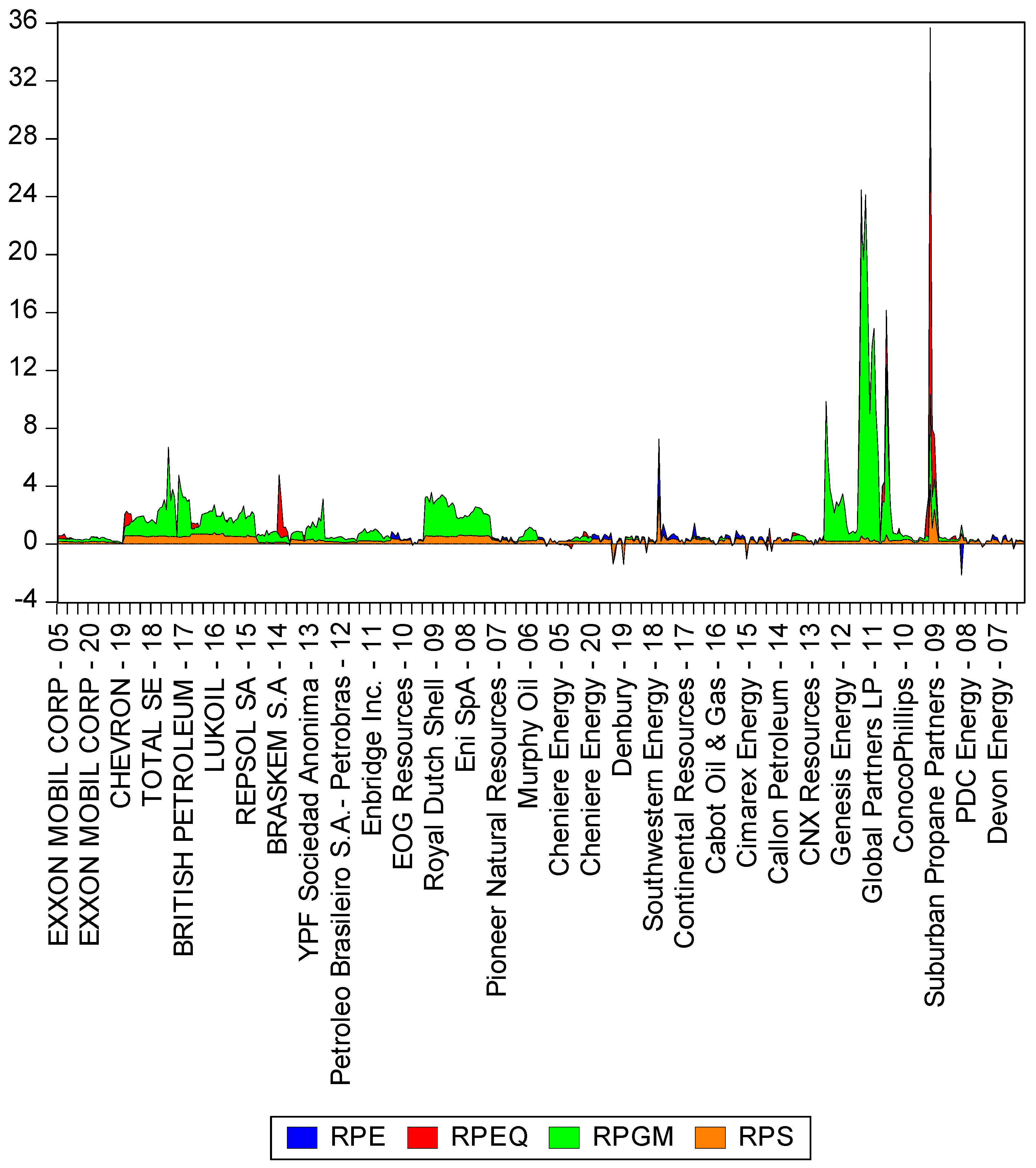
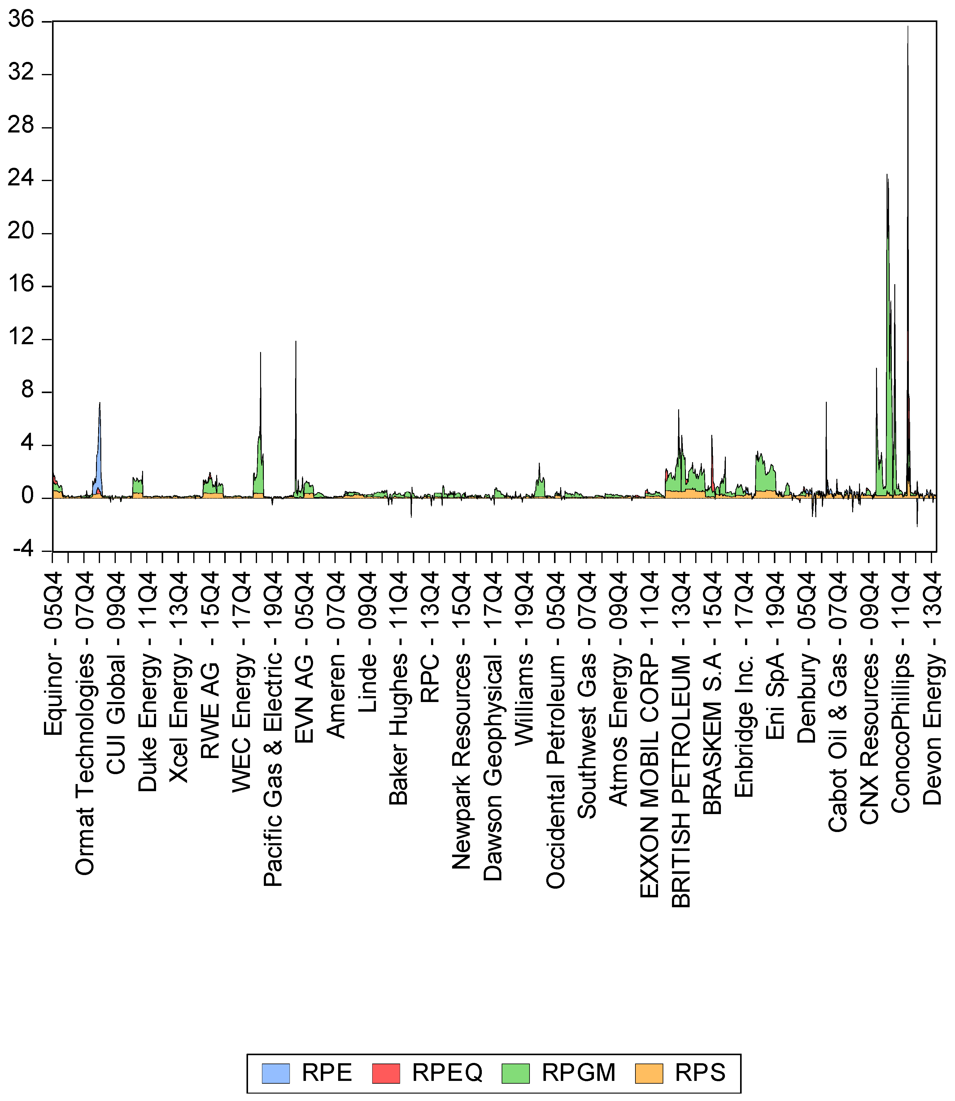
Fiscal pressure to gross margin ratio (RPGM), determined by dividing excises and income tax to gross margin. The indicator highlights the level of own resources allocated by a company to meet taxation requirements;

5.

Fiscal pressure to equity ratio (RPEQ), calculated by dividing excises and income tax to equity. The indicator shows the capacity of the company to meet mandatory fiscal obligations based on its equity;

6.

Fiscal pressure to sales (RPS), calculated as a ratio of taxation to sales. The indicator shows the capacity of a company to pay fiscal obligations from its sales;

7.

Fiscal pressure to expenses (RPE), computed as a ratio of taxation to total expenses of the company.

Financial data used to compute the variables of interest were retrieved from the yearly financial statements of the energy companies, which were published on the NYSE webpage.

In order to investigate the relationship between the chosen indicators, it was necessary to identify particularities in the evolution of data for the specified time span. As a first step, I analyzed the individual evolution of indicators for each company type. Figure 1 displays the equilibrium indicators of electricity companies.

As can be seen from Figure 1, the liquidity state of electricity companies registered constant increases across the entire period, especially after the end of the financial crisis. At the same time, the evolution of the debt to equity ratio was constant, except for the period 2016–2017 when two American companies (i.e., Qrmat Technologies, Texas Pacific Land) registered considerable increases.

Figure 2 displays the evolution of the liquidity and solvency indicators for the gas companies.

Figure 2 shows that the equilibrium indicators of gas companies registered slight fluctuations across the analyzed period. Nevertheless, the overall trend showed a positive increase from one year to the other. In particular, gas companies from the USA registered higher liquidity levels as compared to other companies.

Furthermore, an analysis of the evolution of financial equilibrium for oil companies was also conducted.

From the data presented in Figure 3, it can be seen that solvency indicators corresponding to companies operating in Spain and the USA registered the highest increases over the entire period analyzed. Last but not least, Figure 4 shows the equilibrium trend of all companies included in the sample.

According to Figure 4, solvency level was considerably high in the case of companies such as Ormat Technologies, WEC Energy, Braskem SA, Eni SpA, and Cabot Oil & Gas.

In the following, I have also focused on the evolution of fiscal pressure indicators for all types of companies and for the overall sample.

From an economic point of view, Figure 5 illustrates the fact that, in the case of the 30 electricity companies, fiscal pressure indicators had a non-monotonic evolution throughout the 16-year period.

In case of the 29 gas companies, Figure 6 shows that the level of fiscal pressure indicators had a monotonic evolution as compared to electricity companies (see Figure 5).

According to Figure 7, the 29 oil companies registered a non-monotonic evolution of their fiscal pressure indicators during the analyzed period.

Again, Figure 8 illustrates the fact that, in the case of all 88 energy companies, fiscal pressure indicators had a non-monotonic evolution throughout the 16 years.

4. Results

4.1. Analysis of Central Tendency and Variation

The measures of central tendency (mean, median, standard deviation) were computed for all variables of interest: current liquidity ratio (CR); quick ratio (QR); debt to equity ratio (D/E); fiscal pressure to gross margin ratio (RPGM); fiscal pressure to equity ratio (RPEQ); fiscal pressure to sales ratio (RPS); fiscal pressure to expenses ratio (RPE).

Table 1. Descriptive statistics for electricity companies.

	CR	QR	D/E	RPE	RPEQ	RPGM	RPS
Mean	2.0596	1.5029	2.6900	0.2682	0.2497	0.4474	0.1479
Median	0.9100	0.7100	2.3700	0.1110	0.0891	0.1579	0.0865
Maximum	70.9800	67.6759	48.4900	7.2488	11.0196	11.8650	0.5704
Minimum	0.0000	0.0000	–1.7700	–0.1005	–0.5079	–0.2565	–0.1598
Std. dev.	6.7087	4.9829	2.6352	0.6450	0.6172	0.8437	0.1389
Skewness	7.2430	9.2367	11.5093	7.6216	11.6726	6.9473	1.2118
Kurtosis	61.1622	103.5865	192.8383	70.0098	195.3905	78.3583	3.3238
Jarque–Bera	71,853.69 ***	209,178.1 ***	731,368.4 ***	94,453.34 ***	751,182.5 ***	117,438.6 ***	119.5688 ***
Observations	480	480	480	480	480	480	480

Note: *** indicates significance at the 1% level.

displays the measures of central tendency and variation for electricity companies.

Table 1 presents the mean, median, and standard deviation corresponding to electricity companies. Based on the standard deviation, one can see that QR and CR had the largest volatility, while RPS had the smallest volatility. According to the skewness values, all seven variables were skewed to the right. Since the kurtosis values of all variables were above 3, their distributions were leptokurtic.

The Jarque–Bera test investigates the normal distribution of empirical data. Under the null hypothesis, data are normally distributed. When the probability associated with the Jarque–Bera test exceeds the chosen significance level (be it 1%, 5%, or 10%), the null hypothesis is accepted. As indicated by the test, the seven variables of interest were non-normally distributed at the 1% level.

Table 2. Descriptive statistics for gas companies.

	CR	QR	D/E	RPE	RPEQ	RPGM	RPS
Mean	1.6745	1.2925	1.3986	0.0966	0.1291	0.2628	0.0759
Median	1.4500	1.1400	1.3350	0.0829	0.1072	0.2362	0.0707
Maximum	9.9400	9.1371	11.2000	0.5232	1.0408	2.6704	0.3020
Minimum	0.0000	0.0000	–54.5200	–0.2343	–0.1319	–1.4322	–0.2073
Std. dev.	1.0085	0.8464	2.8016	0.0891	0.1556	0.2918	0.0595
Skewness	2.0151	2.5548	–17.0448	1.7508	3.6054	2.0833	0.5249
Kurtosis	12.5368	18.9359	343.9065	8.4817	19.5711	19.2487	7.0256
Jarque–Bera	2,072.397 ***	5,414.521 ***	2,269,333 ***	817.9810 ***	6,314.202 ***	5,440.004 ***	334.6165 ***
Observations	464	464	464	464	464	464	464

Note: *** indicates significance at the 1% level.

displays the descriptive statistics for gas companies. According to the standard deviation, D/E and CR had the largest volatility, while RPS had again the smallest volatility. Six variables were skewed to the right and D/E was skewed to the left. Since kurtosis values for all variables were above 3, their distributions were leptokurtic. Moreover, the Jarque–Bera test indicated that all variables were non-normally distributed at the 1% level.

In

Table 3. Descriptive statistics for oil companies.

	CR	QR	D/E	RPE	RPEQ	RPGM	RPS
Mean	1.3262	1.0868	1.8761	0.3688	0.9196	1.2542	0.2943
Median	1.1900	0.9400	1.2300	0.2754	0.2868	0.4376	0.2324
Maximum	14.2100	13.9765	43.8200	7.2552	35.6649	24.1177	4.1195
Minimum	0.0000	0.0000	–17.8500	–2.1492	–1.3598	–1.4106	–1.3769
Std. dev.	1.0384	1.0426	3.8104	0.4819	2.7809	2.5141	0.3339
Skewness	7.5879	7.7845	4.5923	7.8821	7.6966	5.5094	4.6981
Kurtosis	77.6372	79.0535	48.5739	107.2933	75.8318	40.4130	56.7641
Jarque–Bera	111,911.3 ***	116,261.8 ***	41,695.78 ***	215,094.9 ***	106,903.1 ***	29,408.87 ***	57,591.56 ***
Observations	463	463	463	464	463	464	464

Note: *** indicates significance at the 1% level.

, one can see the descriptive statistics for oil companies. The standard deviation indicated that D/E and RPEQ had the largest volatility, while RPS had the smallest volatility. All variables were skewed to the right and had leptokurtic distributions. The Jarque–Bera test showed that all variables were non-normally distributed at the 1% level.

Table 4. Descriptive statistics for all companies.

	CR	QR	D/E	RPE	RPEQ	RPGM	RPS
Mean	1.6912	1.2966	1.9963	0.2448	0.4304	0.6525	0.1724
Median	1.1100	0.8800	1.6300	0.1216	0.1203	0.2655	0.1013
Maximum	70.9800	67.6759	48.4900	7.2552	35.6649	24.1177	4.1195
Minimum	0.0000	0.0000	–54.5200	–2.1492	–1.3598	–1.4322	–1.3769
Std. dev.	4.0140	3.0135	3.1636	0.4829	1.6730	1.5919	0.2293
Skewness	11.8212	14.5247	0.9601	9.0865	12.5941	8.3908	5.9315
Kurtosis	166.7452	267.7619	139.3414	114.7421	205.1669	96.0584	95.3250
Jarque–Bera	1,604,651 ***	4,159,018 ***	1,089,994 ***	751,903.8 ***	2,433,282 ***	524,567.1 ***	508,324.9 ***
Observations	1407	1407	1407	1408	1407	1408	1408

Note: *** indicates significance at the 1% level.

displays the descriptive statistics for all energy companies included in the sample. As shown by the standard deviation, CR and D/E registered the largest volatility and RPS the smallest volatility. Again, all variables were skewed to the right, with leptokurtic distributions, and were non-normally distributed at the 1% level.

Table 5. Average values for the overall sample and each energy sector.

Indicators	Electricity Companies	Gas Companies	Oil Companies	Overall Sample
Current ratio (CR)	205.96%	167.45%	132.62%	169.12%
Quick ratio (QR)	150.29%	129.25%	108.68%	129.66%
Debt to equity ratio (D/E)	269.00%	139.86%	187.61%	199.63%

displays the average values for liquidity and solvency indicators.

Table 5 emphasizes similarities and differences between the electricity, gas, and oil companies included in the company sample. For all companies, the current ratio registered average values within the financial security gap of 100%–250%, which is specific for the energy industry. Moreover, average quick ratio values of all companies belonged to the range of 100%–150%, which is typical for the energy industry. Concerning the debt to equity ratio, average values fell between 140% and 270%, which may have caused problems when trying to meet fiscal and commercial debts. At the same time, the average solvency level of gas companies was lower as compared to electricity and oil companies. Namely, the volume of bank loans contracted by gas companies was lower than the volume contracted by electricity and oil companies.

4.2. Correlation Analysis

This study employed a panel model to investigate the relationships between variables. First and foremost, a correlation analysis was run in order to control for potential multicollinearity problems that could bias empirical results.

Table 6. Correlation matrix for electricity companies.

	CR	QR	D/E	RPE	RPEQ	RPGM	RPS
CR	1
QR	0.901	1
D/E	–0.154	–0.146	1
RPE	0.751	0.873	–0.126	1
RPEQ	0.039	0.051	0.706	0.190	1
RPGM	–0.024	–0.019	0.239	0.099	0.515	1
RPS	0.184	0.177	0.016	0.427	0.541	0.520	1

illustrates the pairwise Pearson correlation coefficients for the electricity companies.

The outcome variables CR and QR were negatively correlated with RPGM and positively correlated with the RPE, RPEQ, and RPS fiscal pressure indicators. D/E was positively correlated with RPEQ, RPGM, and RPS and negatively correlated with RPE. The highest correlation among our predictors was registered between RPS and RPEQ (r = 0.541), which nevertheless had a moderate value. Since none of the correlations between two predictors exceeded the value of 0.9, it can be concluded that multicollinearity would pose no problem for the econometric estimations.

Analyzing the results from

Table 7. Correlation matrix for gas companies.

	CR	QR	D/E	RPE	RPEQ	RPGM	RPS
CR	1
QR	0.941	1
D/E	–0.173	–0.160	1
RPE	–0.079	–0.033	–0.018	1
RPEQ	0.044	0.039	0.089	0.250	1
RPGM	0.037	0.030	0.027	0.244	0.765	1
RPS	–0.072	–0.038	–0.008	0.924	0.343	0.364	1

the following aspects were identified. RPE and RPS were negatively correlated with liquidity and solvency indicators, while RPEQ and RPGM were positively correlated. Except for the correlation between the predictors RPS and RPE, no other strong correlations were registered. Hence, the problem of multicollinearity was ruled out for gas companies.

According to

Table 8. Correlation matrix for oil companies.

	CR	QR	D/E	RPE	RPEQ	RPGM	RPS
CR	1
QR	0.988	1
D/E	0.048	0.035	1
RPE	–0.042	–0.068	–0.071	1
RPEQ	0.008	–0.051	0.168	0.456	1
RPGM	–0.009	–0.073	0.092	0.247	0.832	1
RPS	0.027	–0.007	–0.052	0.847	0.520	0.334	1

, the solvency indicator was negatively correlated with RPE and RPS. Current ratio was positively correlated with RPEQ and RPS, while quick ratio was negatively correlated with all predictors measuring fiscal pressure. Since none of the correlations between two fiscal pressure indicators was above 0.9, the problem of multicollinearity was ruled out.

When considering all 88 energy companies (

Table 9. Correlation matrix for all companies.

	CR	QR	D/E	RPE	RPEQ	RPGM	RPS
CR	1
QR	0.904	1
D/E	–0.073	–0.070	1
RPE	0.610	0.701	–0.054	1
RPEQ	–0.002	–0.008	0.186	0.279	1
RPGM	–0.023	–0.030	0.096	0.188	0.813	1
RPS	0.050	0.048	–0.014	0.564	0.534	0.422	1

), all correlations established between predictors were below the critical threshold of 0.9. Hence, it can be concluded that multicollinearity would pose no problem for the econometric estimations.

4.3. Econometric Models

The EViews software version 9.0 was used to estimate econometric models via Panel Least Squares (with cross-section weights) in order to analyze the relationships between fiscal pressure and equilibrium indicators on the sample of 88 energy companies listed on the New York Stock Exchange.

In accordance with Baltagi [26], the first step in analyzing panel data is to decide whether one should run a panel model or a regular regression model. For this purpose, I used the redundant fixed effects tests, namely the cross-section F-test and the cross-section chi-square test. The p-values associated with these two tests were below 0.001, meaning that the null hypothesis according to which individual effects are redundant must be rejected. Hence, individual effects should be included.

The next step would be to choose between fixed and random effects. In this sense, the Hausman test was conducted in order to determine the appropriate type of effects to be chosen for the econometric models. The null hypothesis for the Hausman test assumes that there are no significant differences between the coefficients estimated with the fixed effects model and those estimated with the random effects model; therefore, the random effects model is recommended. If the null hypothesis is rejected, the model with fixed effects should be used.

Concerning the present study, since the p-value associated with the Hausman test was below 0.05, the hull hypothesis was rejected and the fixed effects models were singled out as appropriate to test the hypotheses. Moreover, the variance-covariance matrix of the estimators was determined with the White cross-section method to control for heteroscedasticity at transversal level.

Empirical research was based on the following research hypotheses:

Hypothesis 1 (H1).

There is a linear relationship between fiscal pressure and liquidity.

Hypothesis 2 (H2).

There is a linear relationship between fiscal pressure and solvency.

All econometric models estimated in this study had the following format:

$$B_{it }=a_0+a_1{A}_{1 it}+a_2{A}_{2it}+a_3{A}_{3it}+a_4{A}_{4it}+ {\theta }_t+{\epsilon }_{it}$$

in which:

• $a_0$ represents the intercept;
• $a_i$ represents the coefficient of the predictors;
• A represents the predictors;
• i refers to the company activity;
• t refers to the time frame considered;
• ${\theta }_t$ represents fixed effects controlling for financial crises;
• ${\epsilon }_{it}$ refers to the error term.

Considering that the global financial crisis impacted on the variables of interest, relationships were investigated also without time fixed effects.

Table 10. Econometric models corresponding to the dependent variables CR, QR, and D/E for electricity companies.

	Model E1: $\mathit{C}\mathit{R}={\mathit{a}}_0+{\mathit{a}}_1\mathit{R}\mathit{P}\mathit{E}+{\mathit{a}}_2\mathit{R}\mathit{P}\mathit{E}\mathit{Q}+{\mathit{a}}_3\mathit{R}\mathit{P}\mathit{G}\mathit{M}+{\mathit{a}}_4\mathit{R}\mathit{P}\mathit{S}$		Model E2: $\mathit{Q}\mathit{R}={\mathit{a}}_0+{\mathit{a}}_1\mathit{R}\mathit{P}\mathit{E}+{\mathit{a}}_2\mathit{R}\mathit{P}\mathit{E}\mathit{Q}+{\mathit{a}}_3\mathit{R}\mathit{P}\mathit{G}\mathit{M}+{\mathit{a}}_4\mathit{R}\mathit{P}\mathit{S}$		Model E3: $\mathit{D}/\mathit{E}={\mathit{a}}_0+{\mathit{a}}_1\mathit{R}\mathit{P}\mathit{E}+{\mathit{a}}_2\mathit{R}\mathit{P}\mathit{E}\mathit{Q}+{\mathit{a}}_3\mathit{R}\mathit{P}\mathit{G}\mathit{M}+{\mathit{a}}_4\mathit{R}\mathit{P}\mathit{S}$
Constant	1.4812 *** (2.9210)	1.6635 *** (2.9715)	2.2655 *** (3.1206)	2.3238 *** (3.1484)	3.8851 *** (6.1474)	3.6299 *** (5.7803)
$RPE$	2.6029 (1.2065)	2.6366 (1.2081)	6.0328 *** (3.6193)	6.0341 *** (3.5944)	0.0123 (0.0815)	0.0185 (0.1161)
$RPEQ$	–0.2623 * (–1.6567)	–0.3920 * (–1.7460)	–0.1418 * (–1.7775)	–0.2113 ** (–2.2649)	4.1549 *** (12.1410)	4.1892 *** (14.1019)
$RPGM$	0.0766* (1.9268)	0.0967 (1.1230)	0.0322 (0.4960)	0.0381 (0.5269)	–0.1311 (–1.1679)	–0.1279 (–1.1207)
RPS	–0.5984 (–0.0987)	–1.7340 (–0.2665)	–15.9555 *** (–2.6556)	–16.2532 *** (–2.6300)	–14.7234 *** (–3.4106)	–13.0765 *** (–2.9314)
White cross-section standard errors & covariance (d.f. corrected)	Yes	Yes	Yes	Yes	Yes	Yes
Prob. > F	0.0000	0.0000	0.0000	0.0000	0.0000	0.0000
Cross-section effects	Yes	Yes	Yes	Yes	Yes	Yes
Time fixed effects	No	Yes	No	Yes	No	Yes
R2	0.8033	0.8109	0.8518	0.8578	0.8385	0.8509
Adjusted R2	0.7888	0.7898	0.8409	0.8420	0.8265	0.8343
F-statistic	55.2066	38.4967	77.7054	54.1736	70.1556	51.2486
Observations	480	480	480	480	480	480

Note: Robust t-statistics are indicated in parentheses. *, **, *** denote statistical significance at the 10%, 5%, and 1% levels. Prob. > F is the probability of not including fixed effects. For all econometric models, the variance inflation test values registered levels below 2; hence, multicollinearity was not regarded as a potential bias. The White test rejected the null hypothesis of heteroscedasticity.

,

Table 11. Econometric models corresponding to the dependent variables CR, QR, and D/E for gas companies.

	Model G1: $\mathit{C}\mathit{R}={\mathit{a}}_0+{\mathit{a}}_1\mathit{R}\mathit{P}\mathit{E}+{\mathit{a}}_2\mathit{R}\mathit{P}\mathit{E}\mathit{Q}+{\mathit{a}}_3\mathit{R}\mathit{P}\mathit{G}\mathit{M}+{\mathit{a}}_4\mathit{R}\mathit{P}\mathit{S}$		Model G2: $\mathit{Q}\mathit{R}={\mathit{a}}_0+{\mathit{a}}_1\mathit{R}\mathit{P}\mathit{E}+{\mathit{a}}_2\mathit{R}\mathit{P}\mathit{E}\mathit{Q}+{\mathit{a}}_3\mathit{R}\mathit{P}\mathit{G}\mathit{M}+{\mathit{a}}_4\mathit{R}\mathit{P}\mathit{S}$		Model G3: $\mathit{D}/\mathit{E}={\mathit{a}}_0+{\mathit{a}}_1\mathit{R}\mathit{P}\mathit{E}+{\mathit{a}}_2\mathit{R}\mathit{P}\mathit{E}\mathit{Q}+{\mathit{a}}_3\mathit{R}\mathit{P}\mathit{G}\mathit{M}+{\mathit{a}}_4\mathit{R}\mathit{P}\mathit{S}$
Constant	1.8333 *** (31.9986)	1.8179 *** (28.1981)	1.4618 *** (28.2845)	1.4265 *** (24.5352)	1.0552 ** (2.2812)	0.7973 * (1.7733)
$RPE$	0.4764 (0.5270)	0.5423 (0.5792)	0.1944 (0.2384)	0.2499 (0.2959)	–3.0060 (–1.1108)	–3.0752 (–1.0832)
$RPEQ$	–0.3457 (–0.9271)	–0.1620 (–0.4001)	–0.6133 * (–1.8236)	–0.4889 (–1.3390)	4.3765 ** (2.2077)	5.6715 ** (2.5403)
$RPGM$	–0.7181 *** (–3.7462)	–0.7548 *** (–3.8159)	–0.6814 *** (–3.9403)	–0.6655 *** (–3.7303)	–0.5104 (–1.5252)	–0.6250 (–1.5622)
RPS	0.374914 (0.256514)	0.3091 (0.2067)	0.9235 (0.7005)	1.0507 (0.7790)	2.6754 (0.5239)	4.3545 (0.6668)
White cross-section standard errors & covariance (d.f. corrected)	Yes	Yes	Yes	Yes	Yes	Yes
Prob. > F	0.0000	0.0000	0.0000	0.0000	0.0001	0.0000
Cross-section effects	Yes	Yes	Yes	Yes	Yes	Yes
Time fixed effects	No	Yes	No	Yes	No	Yes
R2	0.6935	0.6992	0.6459	0.6527	0.1499	0.1957
Adjusted R2	0.6707	0.6652	0.6196	0.6134	0.0868	0.1049
F-statistic	30.4735	20.5770	24.5687	16.6322	2.3751	2.1540
Observations	464	464	464	464	464	464

Note: Robust t-statistics are indicated in parentheses. *, **, *** denote statistical significance at the 10%, 5%, and 1% levels. Prob. > F is the probability of not including fixed effects. For all econometric models, the variance inflation test values registered levels below 7; hence, multicollinearity was not regarded as a potential bias. The White test rejected the null hypothesis of heteroscedasticity.

,

Table 12. Econometric models corresponding to the dependent variables CR, QR, and D/E for oil companies.

	Model O1: $\mathit{C}\mathit{R}={\mathit{a}}_0+{\mathit{a}}_1\mathit{R}\mathit{P}\mathit{E}+{\mathit{a}}_2\mathit{R}\mathit{P}\mathit{E}\mathit{Q}+{\mathit{a}}_3\mathit{R}\mathit{P}\mathit{G}\mathit{M}+{\mathit{a}}_4\mathit{R}\mathit{P}\mathit{S}$		Model O2: $\mathit{Q}\mathit{R}={\mathit{a}}_0+{\mathit{a}}_1\mathit{R}\mathit{P}\mathit{E}+{\mathit{a}}_2\mathit{R}\mathit{P}\mathit{E}\mathit{Q}+{\mathit{a}}_3\mathit{R}\mathit{P}\mathit{G}\mathit{M}+{\mathit{a}}_4\mathit{R}\mathit{P}\mathit{S}$		Model O3: $\mathit{D}/\mathit{E}={\mathit{a}}_0+{\mathit{a}}_1\mathit{R}\mathit{P}\mathit{E}+{\mathit{a}}_2\mathit{R}\mathit{P}\mathit{E}\mathit{Q}+{\mathit{a}}_3\mathit{R}\mathit{P}\mathit{G}\mathit{M}+{\mathit{a}}_4\mathit{R}\mathit{P}\mathit{S}$
Constant	1.3448 *** (25.1243)	1.3766 *** (23.0901)	1.1190 *** (19.0453)	1.1460 *** (19.4428)	2.7027 *** (6.2697)	2.3003 *** (11.5668)
$RPE$	–0.3314 * (–1.6926)	–0.3668 (–1.5647)	–0.4019 ** (–2.2341)	–0.4300 ** (–1.9931)	–1.1688 (–1.5901)	–0.5547 (–0.8105)
$RPEQ$	0.0189 (1.1056)	0.0290 (1.2934)	0.0191 (1.1180)	0.0269 (1.2266)	0.6550 ** (2.1664)	0.5529 * (1.8182)
$RPGM$	–0.0236 * (–1.6160)	–0.0353 * (–1.7731)	–0.0232 * (–1.7934)	–0.0321 * (–1.7479)	–0.4141 (–1.5725)	–0.2772 (–1.0672)
$RPS$	0.3848 (1.4086)	0.3363 (0.9983)	0.4217 * (1.7954)	0.3760 (1.2590)	–1.7284 * (–1.6598)	–1.3543 (–1.3672)
White cross-section standard errors & covariance (d.f. corrected)	Yes	Yes	Yes	Yes	Yes	Yes
Prob. > F	0.0000	0.0000	0.0000	0.0000	0.0000	0.0000
Cross-section effects	Yes	Yes	Yes	Yes	Yes	Yes
Time fixed effects	No	Yes	No	Yes	No	Yes
R2	0.4203	0.4375	0.4338	0.4535	0.1973	0.2352
Adjusted R2	0.3772	0.3738	0.3916	0.3916	0.1376	0.1486
F-statistic	9.7432	6.8687	10.2941	7.3262	3.3036	2.7155
Observations	463	463	463	463	463	463

Note: Robust t-statistics are indicated in parentheses. *, **, *** denote statistical significance at the 10%, 5%, and 1% levels. Prob. > F is the probability of not including fixed effects. For all econometric models, the variance inflation test values registered levels below 5; hence, multicollinearity was not regarded as a potential bias. The White test rejected the null hypothesis of heteroscedasticity.

and

Table 13. Econometric models corresponding to the dependent variables CR, QR, and D/E for all energy companies.

	Model A1: $\mathit{C}\mathit{R}={\mathit{a}}_0+{\mathit{a}}_1\mathit{R}\mathit{P}\mathit{E}+{\mathit{a}}_2\mathit{R}\mathit{P}\mathit{E}\mathit{Q}+{\mathit{a}}_3\mathit{R}\mathit{P}\mathit{G}\mathit{M}+{\mathit{a}}_4\mathit{R}\mathit{P}\mathit{S}$		Model A2: $\mathit{Q}\mathit{R}={\mathit{a}}_0+{\mathit{a}}_1\mathit{R}\mathit{P}\mathit{E}+{\mathit{a}}_2\mathit{R}\mathit{P}\mathit{E}\mathit{Q}+{\mathit{a}}_3\mathit{R}\mathit{P}\mathit{G}\mathit{M}+{\mathit{a}}_4\mathit{R}\mathit{P}\mathit{S}$		Model A3: $\mathit{D}/\mathit{E}={\mathit{a}}_0+{\mathit{a}}_1\mathit{R}\mathit{P}\mathit{E}+{\mathit{a}}_2\mathit{R}\mathit{P}\mathit{E}\mathit{Q}+{\mathit{a}}_3\mathit{R}\mathit{P}\mathit{G}\mathit{M}+{\mathit{a}}_4\mathit{R}\mathit{P}\mathit{S}$
Constant	1.4739 *** (9.7149)	1.4542 ** (8.8516)	0.9236 *** (7.4013)	0.8739 *** (5.1947)	2.6974 *** (6.6836)	2.5817 *** (7.7558)
$RPE$	2.1623 (1.1498)	2.1493 (1.1366)	4.7689 *** (2.9129)	4.7617 *** (2.9003)	–0.2357 * (–1.7109)	–0.2412 * (–1.7963)
$RPEQ$	–0.0811 * (–1.8527)	–0.1007 * (–1.9501)	–0.1030 * (–1.6766)	–0.1278 * (–1.8854)	1.0341 * (1.8831)	0.9755 * (1.7814)
$RPGM$	0.0414 (1.3692)	0.0558 (1.3745)	0.0617 (1.4864)	0.0897 * (1.7698)	–0.5461 (–1.4695)	–0.4822 (–1.3231)
$RPS$	–1.7223 (–0.9287)	–1.5939 (–0.8898)	–4.5030 *** (–2.6191)	–4.2449 *** (–2.5571)	–4.3134 * (–1.9510)	–3.7224 * (–1.7495)
White cross-section standard errors & covariance (d.f. corrected)	Yes	Yes	Yes	Yes	Yes	Yes
Prob. > F	0.0000	0.0000	0.0000	0.0000	0.0000	0.0000
Cross-section effects	Yes	Yes	Yes	Yes	Yes	Yes
Time fixed effects	No	Yes	No	Yes	No	Yes
R2	0.7887	0.7921	0.7906	0.7949	0.2643	0.2783
Adjusted R2	0.7740	0.7752	0.7761	0.7782	0.2134	0.2195
F-statistic	53.9295	46.7285	54.5520	47.5425	5.1909	4.7294
Observations	1407	1407	1407	1407	1407	1407

Note: Robust t-statistics are indicated in parentheses. *, **, *** denote statistical significance at the 10%, 5% and 1% levels. Prob. > F is the probability of not including fixed effects. For all econometric models, the variance inflation test values registered levels below 3; hence, multicollinearity was not regarded as a potential bias. The White test rejected the null hypothesis of heteroscedasticity.

present the econometric models for each energy sector and for the overall sample.

The following paragraphs report on the estimated outcomes for the sample of electricity companies.

When time fixed effects were not considered, model E1 revealed that 78.88% of the variance in current liquidity ratio was due to the effect of RPEQ and RPGM fiscal pressure indicators (F = 55.21, p < 0.001). Namely, according to results, a one-unit change in RPEQ generated a 0.262-unit decrease in current ratio. A one-unit change in RPGM generated a 0.077-unit increase in current ratio. The other two fiscal pressure indicators (RPE and RPS) did not have a significant influence on this liquidity outcome. In the case of time fixed effects (F = 38.50, p < 0.001), only RPEQ had a significant negative influence on current ratio and explained 78.98% of its variance. If RPEQ augmented by one unit, the current liquidity would decrease considerably by 0.392 units.

In model E2 with no time fixed effects, fiscal pressure to expenses, fiscal pressure to equity and fiscal pressure to sales ratios significantly influenced quick ratio (F = 77.71, p < 0.001). In other words, when RPE registered a growth of one unit, and the quick ratio increased by 6.033 units. Provided that the variable RPEQ rose by one unit, quick liquidity would decrease by 0.142 units. Last but not least, a one-unit increase in RPS would be followed by a substantial 15.956-unit decrease in liquidity. The value of the adjusted R² indicated that 84.09% of the variance in quick ratio was caused by the three aforementioned factors. After running the model with time fixed effects (F = 54.17, p < 0.001), the same fiscal pressure indicators triggered significant changes in quick ratio. This time, the impact of fiscal pressure to sales was even stronger. The three fiscal pressure indicators accounted for 84.20% of the total variance.

Model E3 revealed that, in the case of no time fixed effects, the influences of the independent variables RPEQ and RPS on the solvency indicator were significant and noteworthy (F = 70.16, p < 0.001). In terms of the impact triggered by RPEQ, when this indicator augmented by one unit, solvency would increase by 4.155 units. In addition, if RPS augmented by one unit, solvency would mitigate by 14.72 units. Introducing time fixed effects into the model yielded similar results concerning the influence of fiscal pressure indicators (F = 51.25, p < 0.001), which explained 83.43% of the variance.

Table 11 displays the econometric models estimating the relationship between fiscal pressure, liquidity, and solvency on the gas company sample.

According to model G1 with no time effects, which explained 67.07% of the total variance in current liquidity ratio (F = 30.47, p < 0.001), only RPGM had a significant impact. Namely, a one-unit increase in RPGM would be followed by a 0.718-unit decrease in current liquidity ratio. For the model including time fixed effects, which explained 66.52% of the variance, results were similar (F = 20.58, p < 0.001).

When time fixed effects were not considered, model G2 showed that 61.96% of the variance in quick ratio was due to fiscal pressure indicators (F = 24.57, p < 0.001). Based on the empirical results, RPEQ and RPGM significantly influenced QR. That is, a change of one unit in RPEQ would be followed by a decrease of 0.613 units in QR. Similarly, if RPGM increased by one unit, QR would decrease by 0.618 units. In the case of the time fixed effects model (F = 16.63, p < 0.001) explaining 61.34% of the variance, only RPGM exerted a significant negative impact.

In the case of model G3 without time fixed effects, one could observe that only the influence of fiscal pressure to equity was statistically significant (F = 2.38, p < 0.001). Namely, this indicator explained 8.68% of the variance in solvency. Estimates showed that a one-unit increase in RPEQ would trigger a 4.38-unit increase in the D/E ratio. After running the model with time fixed effects (F = 2.15, p < 0.001), estimations remained roughly the same.

Table 12 presents the econometric models estimating the relationship between fiscal pressure, liquidity, and solvency on the sample of oil companies.

Model O1 without time fixed effects showed that variables RPE and RPGM were statistically significant, with the model explaining 37.72% of the variance in current liquidity ratio (F = 9.74, p < 0.001). Namely, when RPE and RPGM increased by one unit, current liquidity would mitigate by 0.331 and 0.024 units, respectively. The other two fiscal pressure indicators had no impact. In the case of the model with time fixed effects, which explained 37.38% of the variance (F = 6.87, p < 0.001), only RPGM accounted for a significant influence. This time, the size of the change in current liquidity ratio increased a little.

Concerning model O2 with no time fixed effects, RPE, RPGM, and RPS indicators shaped the quick ratio: a one-unit increase in RPE would be followed by a 0.402-unit decrease in QR; should RPGM augment by one unit, QR would mitigate by 0.023 units; if RPS increased by one, QR would follow the same trend with 0.422 units. Based on the value of the adjusted R², 39.16% of the variance in quick ratio can be attributed to the chosen fiscal pressure indicators (F = 10.29, p < 0.001). After introducing the time fixed effects, only RPE and RPGM remained significant, with this second model explaining 39.16% of the variance (F = 7.33, p < 0.001).

Moreover, model O3 (no time fixed effects) reported significant influences of two of the fiscal pressure indicators considered, namely fiscal pressure to equity and fiscal pressure to sales. The model explained 13.76% of the total variance of solvency (F = 3.30, p < 0.001). If RPEQ rose by one unit, solvency would follow a similar trend with 0.655 units. Once RPS increased by one unit, D/E would substantially mitigate by 1.728 units. In addition, the model with time fixed effects reported that RPEQ remained the sole significant variable in relation with debt to equity ratio. This time, the model explained 14.86% of the variance, F = 2.72, p < 0.001.

The relationship between fiscal pressure, liquidity, and solvency was analyzed also for the overall sample of energy companies.

Model A1 with no time fixed effects indicated that the variable RPEQ significantly shaped the current ratio. The econometric model explained 77.40% of the variance in CR (F = 53.93, p < 0.001). Estimates showed that if RPEQ augmented by one unit, liquidity measured with CR would diminish by 0.081 units. After considering the time fixed effects, results remained similar. That is, the model explained 77.52% of the variance (F = 46.73, p < 0.001) and the impact of RPEQ counted the most.

According to model A2 (no time fixed effects), the indicators RPE, RPEQ, and RPS had a significant influence (F = 54.55, p < 0.001). When RPE increased by one unit, quick ratio would follow the same trend with 4.769 units. Similarly, should RPEQ augment by one unit, QR would mitigate by 0.103 units. Last but not least, a one-unit increase in RPS would be followed by a 4.503-unit drop in liquidity. Based on the value of the adjusted R², 77.61% of the variance in liquidity could be attributed to these three fiscal pressure indicators. By including the time fixed effects into the model, it could be noticed that all four fiscal pressure indicators were important (F = 47.54, p < 0.001).

Last but not least, model A3 without any time effects showed that fiscal pressure to expenses, fiscal pressure to equity, and fiscal pressure to sales triggered 21.34% of the variance in solvency (F = 5.19, p < 0.001). In other words, should RPE and RPS increase by one unit, solvency would mitigate by 0.236 and 4.313 units, respectively. For a one-unit increase in RPEQ, solvency would improve by 1.034 units. After considering the time effects (F = 4.73, p < 0.001), 21.95% of the variance in solvency was explained by these three predictors.

5. Discussion

In terms of the electricity companies included in the sample, empirical results showed that the fiscal pressure to equity and fiscal pressure to gross margin ratios significantly influenced the short-term financial equilibrium state measured by the current liquidity ratio (CR). At the same time, in the case of gas companies, the factor that played the most important role in the changes incurred by the current ratio was fiscal pressure to gross margin. For oil companies, significant changes were triggered by the indicators fiscal pressure to expenses and fiscal pressure to gross margin. When investigating the relationship between fiscal pressure and short-term equilibrium on the overall company sample, it turned out that the only substantial impact was driven by fiscal pressure to equity.

Empirical results unraveled that fiscal pressure indicators had both positive and negative influences on the current ratio. In the case of electricity companies, fiscal pressure to gross margin positively influenced current liquidity ratio because for the majority of these companies excises and corporate income tax rates were lower as compared to gas and oil companies from the USA, Germany, Italy, Portugal, Korea, Austria, and Brazil. Thus, lower tax duties increased the current liquidity of these companies. At the same time, for gas and oil companies, fiscal pressure to gross margin had a negative impact on current liquidity ratio. The explanation is straightforward: the high taxation levels (excise, corporate income tax) in these energy sectors lowered company profit and company liquidity.

Concerning quick ratio, panel data analyses showed that all predictors had a certain impact on the evolution of this short-term equilibrium measure. For the subsample of electricity companies, quick ratio was significantly linked to fiscal pressure to expenses, fiscal pressure to equity, and fiscal pressure to sales ratios. Gas companies registered important influences on the account of fiscal pressure to equity and fiscal pressure to gross margin ratios. As for oil companies, the three most significant variables were fiscal pressure to expenses, fiscal pressure to gross margin, and fiscal pressure to sales. Across the entire sample, the factors that played an important role in the changes incurred by quick ratio were fiscal pressure to expenses, fiscal pressure to equity, and fiscal pressure to sales.

Again, the chosen fiscal pressure indicators exerted both positive and negative influences on the quick ratio. For instance, fiscal pressure to equity had a negative influence in the case of electricity companies because these companies have fewer inventories as compared to oil companies. As noted before, across all energy companies, RPEQ and RPS yielded a negative impact on quick ratio, while RPE yielded a positive impact. According to economic theory, the more fiscal pressure increases, the more company liquidity decreases. The positive influence of RPE could be explained as follows: by not taking into account inventories when computing the quick ratio, both receivables and cash levels augment due to low taxation rates applied in the electricity sector.

With respect to solvency measured via debt to equity ratio, fiscal pressure to equity had a positive impact for all energy sectors and for the overall sample. Moreover, fiscal pressure to sales exerted a negative impact for companies from the electricity sector, oil sector, and for the overall company sample.

6. Conclusions

The topic of fiscal pressure and the modeling of this phenomenon is widely debated in the finance literature [27,28,29,30]. Its importance resides in the fact that, depending on the level of taxes, the fiscal pressure triggered by excessive taxation may determine both corporate and individual taxpayers to desist from saving, investing, working, or expanding their lucrative activities. Still, there are no studies regarding the relationship between fiscal pressure and financial equilibrium for publicly traded companies during economic downturns.

The present research study contributes to the existing literature by giving an account of the effects of fiscal pressure on company financial equilibrium through a sample of 30 electricity companies, 29 gas companies, and 29 oil companies listed on the New York Stock Exchange and headquartered in various countries around the world. The time frame selected for the analyses was 2005Q1–2020Q3, which comprised the period before, during and after the 2008 global financial crisis. The relationships between seven indicators measuring company liquidity, solvency, and fiscal pressure were investigated via Panel Least Squares (with cross-section weights) by means of the statistical package EViews version 9.0. Both research hypotheses were confirmed, namely that fiscal pressure indicators had a significant influence on financial liquidity and solvency (i.e., company equilibrium).

The implications of the empirical results for the companies operating in the energy industry are at least threefold from the perspective of this study. To begin with, since the short-term financial equilibrium was strongly and negatively affected by certain fiscal pressure indicators, company managers from this industry should focus more on securing an adequate liquidity level. Strategies such as renegotiating contracts with major suppliers, increasing the inventory turnover, or expanding commercial credits could be put into practice. Moreover, because tax rates following economic downturns display increasing trends, such proactive strategies would be advisable and sensible in the short run. Second, the negative effects of fiscal pressure to sales on company solvency should determine managers to curb companies’ propensity for contracting long-term liabilities. Especially in times of crises, efforts should be made towards decreasing the degree of indebtedness, which might threaten the very existence of a company. Third, as stipulated by economic theory, increasing taxation via excise duties and corporate income tax can generate a reduction of economic activities across the energy sector, which may entail negative consequences for the entire economy. For this reason, governmental authorities need to design fiscal policies that encourage the development of the energy sector, which would benefit the overall society. That is, a larger volume of tax revenues from excise duties and corporate income taxes could be collected following an increase in production of energy companies. Such tax revenues could be further used in the economy by providing the population with higher quality public goods and services.

Among the limitations of the study, one could first mention the number of companies considered from each energy sector. In this sense, future research could expand company subsamples by including other major players in the energy industry, operating on markets especially from South America and Africa. Second, it could be asserted that the significant impact of fiscal pressure on financial equilibrium holds only for companies within the energy industry or for this particular time frame. In this sense, future studies could target various industries from different economic sectors for which to estimate the impact of fiscal pressure on the short and long-term financial equilibrium of major companies in the respective industries. Moreover, stretching the period of time across at least two decades could be considered for the upcoming scientific investigations.

All in all, the current empirical study sheds light on the degree to which fiscal pressure steered the liquidity and solvency levels of companies operating in the energy sector amid and beyond the most recent global financial crisis. That is, the short-term and long-term equilibrium of electricity and oil companies appeared to be more influenced by fiscal pressure than the equilibrium of gas companies. Starting from these results, company managers may estimate the evolution of their equilibrium states when considering other potential financial downturns, similar to this 2008 global financial crisis. It goes without saying that the econometric models advanced in this study can also be applied in the case of the economic crisis that lies ahead of global markets, following the current pandemic. Equipped with such econometric tools, business people will be able to estimate better the company capacity of meeting short and long-term debts and to take proactive measures in order to avoid liquidity crises or even insolvency.

References

1. Fujiwara, I.; Ueda, K. The fiscal multiplier and spillover in a global liquidity trap. J. Econ. Dyn. Control 2013, 37, 1264–1283. [Google Scholar] [CrossRef] [Green Version]
2. Bai, J.; Lu, J.; Li, S. Fiscal pressure, tax competition and environmental pollution. Environ. Resour. Econ. 2019, 73, 431–447. [Google Scholar] [CrossRef]
3. Zhang, Z.; Zhao, W. Research on financial pressure, poverty governance, and environmental pollution in China. Sustainability 2018, 10, 1834. [Google Scholar] [CrossRef] [Green Version]
4. Qi, Y.; Peng, W.; Xiong, N.N. The effects of fiscal and tax incentives on regional innovation capability: Text extraction based on Python. Mathematics 2020, 8, 1193. [Google Scholar] [CrossRef]
5. Batrancea, L.M.; Nichita, R.A.; Batrancea, I.; Moldovan, B.A. Tax compliance models: From economic to behavioral approaches. Transylv. Rev. Adm. Sci. 2012, 8, 13–26. [Google Scholar]
6. Batrancea, L.; Nichita, A.; Batrancea, I.; Gaban, L. The strength of the relationship between shadow economy and corruption: Evidence from a worldwide country-sample. Soc. Indic. Res. 2018, 138, 1119–1143. [Google Scholar] [CrossRef]
7. Batrancea, L.; Nichita, A. Which is the best government? Colligating tax compliance and citizens’ insights regarding authorities’ actions. Transylv. Rev. Adm. Sci. 2015, 11, 5–22. [Google Scholar]
8. Cannell, J. The Financial Crisis and Its Impact on the Electric Utility Industry; Edison Electric Institute: Washington, WA, USA, 2009. [Google Scholar]
9. Mimouni, K.; Temimi, A. What drives energy efficiency? New evidence from financial crises. Energy Policy 2018, 122, 332–348. [Google Scholar] [CrossRef]
10. Altdorfer, F. Impact of the Economic crisis on the EU’s industrial energy consumption. Odysee-Mure Policy Brief. 2017. Available online: https://www.odyssee-mure.eu/publications/policy-brief/impact-economic-crisis-industrial-energy-consumption.pdf (accessed on 14 January 2020).
11. Naeem, M.A.; Balli, F.; Shahzad, S.J.H.; de Bruin, A. Energy commodity uncertainties and the systematic risk of US industries. Energy Econ. 2020, 85, 104589. [Google Scholar] [CrossRef]
12. Schmoll, M. Weak street-level enforcement of tax laws: The role of tax collectors’ persistent but broken public service expectations. J. Dev. Stud. 2021, 57, 209–225. [Google Scholar] [CrossRef]
13. Duernecker, G.; Herrendorf, B. On the allocation of time—A quantitative analysis of the roles of taxes and productivities. Eur. Econ. Rev. 2018, 102, 169–187. [Google Scholar] [CrossRef]
14. Ji, J.; Ye, Z.; Zhang, S. Welfare analysis on optimal enterprise tax rate in China. Econ. Model. 2013, 33, 149–158. [Google Scholar] [CrossRef]
15. Khan, U.; Nallareddy, S.; Rouen, E. The role of taxes in the disconnect between corporate performance and economic growth. Manag. Sci. 2020, 66, 5427–5447. [Google Scholar] [CrossRef] [Green Version]
16. PricewaterhouseCoopers; the World Bank; International Finance Corporation. Paying Taxes 2020: The Changing Landscape of Tax Policy and Administration across 190 Economies; PwC: Washington, WA, USA, 2019. [Google Scholar]
17. Slemrod, J. The consequences of taxation. Soc. Philos. Policy 2006, 23, 73–87. [Google Scholar] [CrossRef]
18. Battiston, P.; Gamba, S. The impact of social pressure on tax compliance: A field experiment. Int. Rev. Law Econ. 2016, 46, 78–85. [Google Scholar] [CrossRef]
19. Listokin, Y. Taxation and liquidity. Yale Law J. 2011, 120, 1682–1732. [Google Scholar]
20. Evans, L.R.; Dewitt, C.K. (Eds.) Fiscal Pressure Facing State & Local Government. American Political, Economic and Security Issues: Government Procedures and Operations; Nova Science Publishers: Hauppauge, NY, USA, 2012. [Google Scholar]
21. Molina-Morales, A.; Amate-Fortes, I.; Guarnido-Rueda, A. Economic and institutional determinants in fiscal pressure: An application to the European case. J. Econ. Issues 2011, 45, 573–592. [Google Scholar] [CrossRef]
22. Villar Rubio, E.; Quesada Rubio, J.M.; Molina Moreno, V. Convergence analysis of environmental fiscal pressure across EU-15 countries. Energy Environ. 2015, 26, 789–802. [Google Scholar] [CrossRef]
23. Trussel, J.M.; Patrick, P.A. Predicting fiscal distress in special district governments. J. Public Budg. Account. Fin. Manag. 2013, 25, 589–616. [Google Scholar] [CrossRef]
24. Ezeoha, A.E.; Ogamba, E. Corporate tax shield or fraud? Insight from Nigeria. Int. J. Law Manag. 2010, 52, 5–20. [Google Scholar] [CrossRef]
25. Bubić, J.; Mladineo, L.; Šušak, T. VAT rate change and its impact on liquidity. Management 2016, 21, 151–166. [Google Scholar]
26. Baltagi, B.H. Econometric Analysis of Panel Data; John Wiley & Sons: Chichester, UK, 2008. [Google Scholar]
27. Man, J. Fiscal pressure, tax competition and the adoption of tax increment financing. Urban Stud. 1999, 36, 1151–1167. [Google Scholar] [CrossRef]
28. U.S. Government Accountability Office. State and Local Governments: Fiscal Pressures Could Have Implications for Future Delivery of Intergovernmental Programs; U.S. Government Accountability Office: Washington, WA, USA, 2019.
29. Wang, R.; Zhang, Q. Local governments’ fiscal pressure and the dependence on polluting industries in China. China World Econ. 2017, 25, 109–130. [Google Scholar] [CrossRef]
30. Liu, S.; Weng, R.; Yang, D. Natural disaster, fiscal pressure and tax avoidance: A typhoon-based study. China J. Account. Stud. 2018, 5, 468–509. [Google Scholar] [CrossRef]
Figure 1. Evolution of equilibrium indicators for electricity companies. Note: The symbol CR denotes the current liquidity ratio, QR denotes the quick ratio, and D/E denotes the debt to equity ratio.
Mathematics 09 00630 g001
Figure 2. Evolution of equilibrium indicators for gas companies.
Mathematics 09 00630 g002
Figure 3. Evolution of equilibrium indicators for oil companies.
Mathematics 09 00630 g003
Figure 4. Evolution of equilibrium indicators for all energy companies in the sample.
Mathematics 09 00630 g004
Figure 5. Evolution of fiscal pressure indicators for electricity companies. Note: The symbol RPE denotes the fiscal pressure to expenses ratio, RPEQ denotes the fiscal pressure to equity ratio, RPGM denotes the fiscal pressure to gross margin ratio, and RPS denotes the fiscal pressure to sales ratio.
Mathematics 09 00630 g005
Figure 6. Evolution of fiscal pressure indicators for gas companies.
Mathematics 09 00630 g006
Figure 7. Evolution of fiscal pressure indicators for oil companies.
Mathematics 09 00630 g007
Figure 8. Evolution of fiscal pressure indicators for all energy companies in the sample.
Mathematics 09 00630 g008