Feature Selection in a Credit Scoring Model

Abstract

This paper proposes different classification algorithms—logistic regression, support vector machine, K-nearest neighbors, and random forest—in order to identify which candidates are likely to default for a credit scoring model. Three different feature selection methods are used in order to mitigate the overfitting in the curse of dimensionality of these classification algorithms: one filter method (Chi-squared test and correlation coefficients) and two wrapper methods (forward stepwise selection and backward stepwise selection). The performances of these three methods are discussed using two measures, the mean absolute error and the number of selected features. The methodology is applied for a valuable database of Taiwan. The results suggest that forward stepwise selection yields superior performance in each one of the classification algorithms used. The conclusions obtained are related to those in the literature, and their managerial implications are analyzed.

1. Introduction

The primary function of banks and financial institutions is to concede credits and loans to households and firms that need funds. Thus, credit risk becomes their most important issue since lending money involves plenty of uncertainties derived from asymmetric information. The credit scoring model, as a form of credit risk management, helps to reduce those uncertainties by evaluating, among other things, the possibility of default when such loans and credits are given. This evaluation process requires a set of features that are necessary to get to know the borrowers better, enabling banks to predict the level of credit risk. However, due to the rapid growth of new technologies and the creation of a vast amount of data on a per-second basis, the need for filtering out irrelevant features to the risk level has increased in recent years. The concept of feature selection, therefore, under these circumstances, has grown in importance to identify a set of significant variables relevant to determine the credit risk of borrowers.

The biggest challenge of building credit scoring models could be to decide which are the most relevant features to be selected for the task. In practice, the data used for the models may be collected from various sources, and sometimes the size of the data is small in relation to the number of features considered, which gives rise to a typical overfitting example. In addition, there might be some features in the data, which may not be significant to credit risk, or some of them may be correlated with each other. Thus, these data issues might result in a misleading interpretation of the credit scoring model and a very poor performance of it.

The feature selection process as a solution to these issues could be considered as a complicated, arbitrary, and unsystematic task since there is no specific theory and the task works differently on different data. Thus, some researchers have come up with several ways that could help sort this ambiguity. For example, some tried univariate analysis [1], such as studying the statistical significance of the predictors on the response variable independently or computing correlation coefficients that determine whether there is a linear dependence between features or not. On top of that, there are classification algorithms that carry out the feature selection process, for example, logistic regression has a parameter called “penalty” to prevent the algorithm from having too many variables included in the model. Other selection methods work in tandem with nonlinear classification algorithms-K-nearest neighbors, support machine vectors, or random forests, such as stepwise selection procedures.

This paper presents a methodology for the selection of the key variables in order to establish a credit scoring model. Different classification algorithms—logistic regression, support vector machine, K-nearest neighbors (KNN), and random forest—are proposed in order to separate data into two classes and identify which candidates are likely to default for this credit scoring. It uses three different feature selection methods in order to mitigate the overfitting in the curse of dimensionality of these classification algorithms, specifically the one filter method (Chi-squared test and correlation coefficients) and two wrapper methods (forward stepwise selection and backward stepwise selection). The performances of these three methods are discussed using two measures, the mean absolute error and the number of selected features. The methodology is applied for a valuable database of Taiwan obtained from Chung Hua University. The results suggest that forward stepwise selection yields superior performance in each one of the classification algorithms used. These results are related and compared to those in the literature, and their managerial implications are analyzed.

The rest of the paper is organized as follows. Section 2 describes the theoretical framework, introducing the concept of credit risk management and including a literature review of the different machine learning techniques used for credit scoring. Section 3 details the methodology proposed to evaluate credit applicants, both the classification algorithms that allow identifying the key features for credit scoring and the different methods used to mitigate the overfitting problem in the practical implementation of these classification algorithms. Section 4 refers to the empirical analysis, describing the sample data and variables used, and analyzing the empirical results obtained from the methodology proposed. Section 5 sums up the conclusions and the implications of the findings.

2. Materials and Methods

2.1. Credit Risk Management

Credit risk can be defined as the possibility that a borrower fails to meet financial obligations. Since on most occasions the main business of banks and other financial institutions involves credits as mentioned before, credit risk management became a crucial tool to alleviate default risk, which allows them to understand sources of the risk. This, in turn, enabled banks to measure the level of risk and to maximize ultimately their rates of return from granting credits. In the last years, there have been different default examples due to poor credit quality of loans and credits conceded by many banks, such as the savings and loan crisis in the late 1980s, crises in countries such as Argentina, Brazil, Russia, and South Korea in the late 1990s, or more recently the subprime crisis that activated the Great Recession [2].

These incidents, therefore, led to various methods for measuring credit risk being developed. Primarily, many financial institutions had been using models that took only into account qualitative factors of borrowers, such as, reputation, leverage, the volatility of earnings, or collateral, and market-specific factors such as the business cycle, currency exchange rates, or interest rates. However, due to the increasing complexity of banking activities, those traditional models were no longer very effective. Quantitative models then started coming to the fore; logit model, methods that use risk premium, Altman’s linear discriminant model, etc. Later, the quantitative models backed up with new technologies, allowed higher-performance credit scoring models that lowered the cost of credit analysis in terms of time and effort and better decision making when granting credits [3]. These recent credit scoring models usually have a form of separating consumers who want to borrow money into two categories (low risk and high risk of default), using various characteristics of the applicants, such as demographic characteristics, economic and financial conditions, etc. The models estimate statistically as close as possible to the current credit risk level. Some popular examples are logistic regression, discriminant analysis, factor analysis, and probit regression and artificial intelligence approaches such as an expert system, neural networks, or support vector machine [4].

2.2. Machine Learning and Credit Scoring: A Review of Literature

Alpaydin [5] defined machine learning as a tool using past data to program computers in order to solve a given problem. Thanks to these advantages machine learning has achieved a dominant position in handling various issues: recognizing speech and handwriting, analyzing past sales data to improve customer relationships, or analyzing the data of clients by financial institutions to predict credit risks. Much literature has been done and is still ongoing about machine learning on credit scoring models out there. Many quantitative techniques have been used in different research to examine the predictive power in credit scoring, from single classifiers (logistic regression, neural networks, K-nearest neighbors, support vector machines, classification trees, etc.) to ensemble methods (random forest, bagging, boosting, etc.). One example of ensemble methods’ development and application is [6]. For an update of the classification algorithms’ research for credit scoring see [7]. Most of these studies rely on a single accuracy or performance measure, or on several measures of the same type. These accuracy measures may split into three general types [7]: those based on a threshold metric (classification error, MAE, etc.), those that assess the discriminatory ability of the scorecard (area under the curve or AUC), and finally those based on a statistical hypothesis testing (paired t-test, Friedman test, analysis of variance, etc.).

Baesens et al. [8] evaluated several single classifiers, compared their performances, and found out that logistic regression and linear discriminant analysis exhibited more outstanding performances in predicting credit risk than the others which were also tested in the paper. Ref. [9] explored eight different machine learning classification algorithms on various real-world datasets and concluded that random forests and logistic regression were the algorithms that had the highest prediction accuracies. However, they emphasized that the details of the problem, the data structure, and the number of features also play a key role in determining the best classifier. On the other hand, ref. [10], their research showed that the combinations of single classification algorithms, that is, ensemble methods, did a better job than single algorithms. Ref. [11] also went through seventy-four studies on statistical and machine learning models for credit scoring to identify the best performing model and found that an ensemble of classifiers had superior performance to single ones. By extension, ref. [12] conducted a feature selection process as a step before implementing classification algorithms. They concluded that after trying four different selection methods—“wrapper”, “consistency-based”, “relieF”, and “correlation-based”—the performance of the K-nearest-neighbors classifier, not the others, improved, no matter which feature selection method was used but especially with the wrapper and consistency-based ones although the KNN was still not the best performing classifier compared to the other algorithms. Tripathi et al. [13] used the ensemble feature selection approach on datasets to which in the next stage a multilayer ensemble classifier was applied to enhance the performance for scoring credit risks. Zhang et al. [14] employed, in order to extract main features, first gradient boosting decision trees (GBDT) for feature transformation and one-hot encoding and then Chi-square statistics to calculate the correlation between features and to select the main ones.

Table 1. Machine learning in credit scoring: classification algorithms and evaluation criteria used.

		Evaluation Criteria
		Threshold Metrics	Statistical Hypothesis Testing	Area under the Curve
Classifier	Logistic regression	[7,12,15]	[9]	[7,16,17]
	Decision tree	[12,15,18]	[9,18]
	Support vector machine (SVM)	[7,8,15]	[8,9]	[7,8,17]
	Artificial neural networks (ANN)	[7,8,12,15]	[8,9]	[7,8]
	Bayesian model	[7]	[9]	[7]
	CART	[7]		[7,16]
	Extreme learning machine (ELM)	[7]		[7]
	K-nearest neighbor (KNN)	[7,12]	[9]	[7]
	Rule induction algorithms		[9]
	Discriminant analysis	[7]		[7]
	Voted perceptron (VP)	[7]		[7]
	Naïve Bayes (NB)	[7]		[7]
	J4.8	[7]		[7]
	Fuzzy logic	[18]	[18]
	Ensemble classifier	[6,7,13,14,15]	[9,10,14]	[6,7,14,16,17]

illustrates empirical literature that measures credit risk using different classification algorithms that employ different evaluation criteria.

3. Methods and Materials

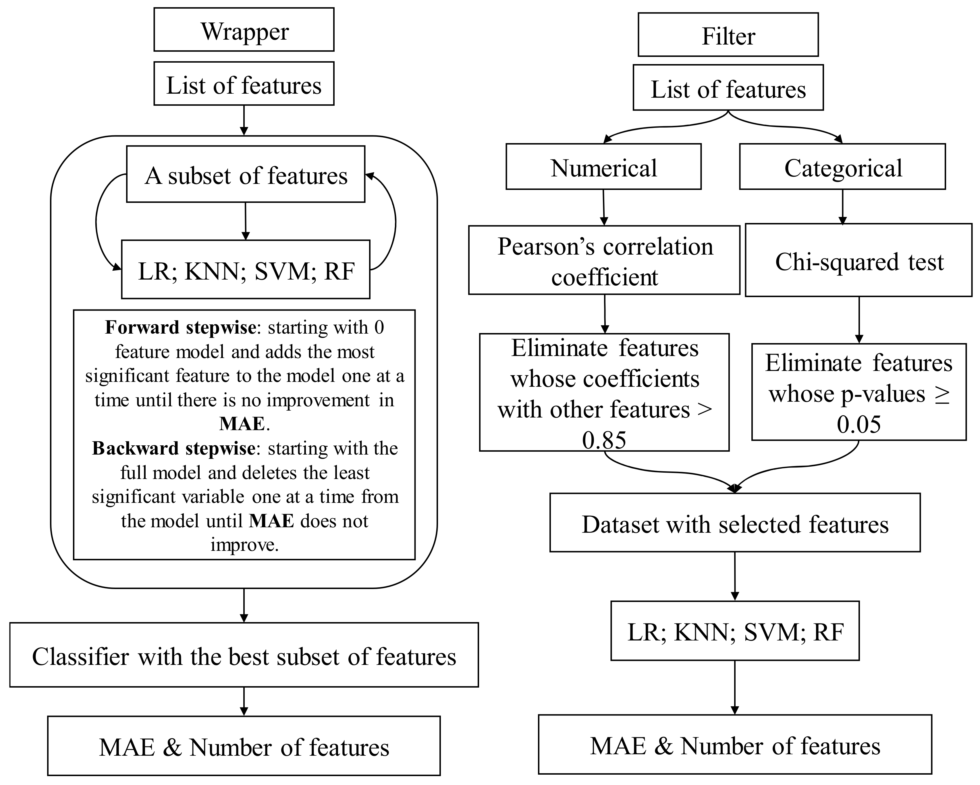
This section presents the methodology proposed to evaluate credit applicants, see Figure 1. Different classification algorithms—logistic regression (LR), support vector machine (SVM), K-nearest neighbors (KNN), and one embedded method, random forest (RF)—were used in order to separate data into two classes and identify which candidates are likely to default for this credit scoring. These classification algorithms were trained with different feature selection methods in order to mitigate the overfitting in the curse of dimensionality of them. Specifically, one filter method (Chi-squared test and correlation coefficients) and two wrapper methods (forward stepwise selection and backward stepwise selection) are used. Then, two performance measures, model simplicity (the number of selected features), and model accuracy (the MAE) were used to see the effects of feature selection by comparing the performance measures before and after the selection process. A resampling method, K-fold cross-validation, is applied to obtain additional information about the fitted model because there is no test data set on which the model can be tested out.

3.1. Classification Algorithms

Next, some of the most representative current mathematical models for implementing credit scoring will be introduced, most of them included within automatic learning techniques.

3.1.1. Logistic Regression

Logistic regression is a particular kind of generalized linear model (GLM) which is a generalization of the concepts of regular linear models. Therefore, logistic regression is not much different from linear regression, but it is used for a classification problem as the one in this analysis.

Y(response) = 0 if a borrower defaults or 1 otherwise

(1)

Logistic regression provides the probability that Y belongs to a specific category so for a binary dependent variable such as this one, the simple linear model using ordinary least squares regression does not make sense since the probability cannot exceed the interval [0, 1]. Instead, the logistic function is used to model the relationship between the response and independent variables. For instance, the probability of Y belonging to class 1 can be written as follows:

$$\mathrm{Pr}\left(Y=1|X\right)=p\left(X\right)=\frac{e^{{\beta }_0+{\beta }_1{X}_1+\cdots +{\beta }_p{X}_p}}{1+e^{{\beta }_0+{\beta }_1{X}_1+\cdots +{\beta }_p{X}_p}}$$

(2)

Since p(X) provides the probability that the response variable is 1, a threshold must exist that classifies data into two or more categories; the default threshold is 0.5, and if a sample whose value of p(X) is equal to or greater than 0.5, it is classified as 1 and 0 otherwise. The logistic function is estimated using the maximum likelihood method and this method finds the coefficients such that plugging these estimated parameters into the model p(X) yields the lowest classification errors.

Although logistic regression cannot yield high accuracy when variables are non-linearly related, it has been commonly used for credit scoring models [19,20,21,22].

3.1.2. Support Vector Machines

Support vector machines (SVM) aim to figure out the best way to separate the classes of data. Observations called support vectors determine the decision boundaries by affecting their positions and maximizing the margins which are the distance between them and the boundaries. To accommodate the non-linearity of boundaries, SVM uses a kernel that generalizes the inner products of the observations and it quantifies the similarity of two observations. A kernel can be denoted as:

$$K\left(x_i,x_{i^{\prime }}\right)={\left(1+{\displaystyle {\displaystyle \sum }_{j=1}^p}{x}_{ij}{x}_{i^{\prime }j}\right)}^d$$

(3)

where d is a degree of the polynomial. According to [23], a very popular choice of the kernel is the radial kernel, and it takes the form:

$$K\left(x_i,x_{i^{\prime }}\right)=\exp (-\gamma {\displaystyle {\displaystyle \sum }_{j=1}^p}{\left(x_{ij}-x_{i^{\prime }j}\right)}^2).$$

(4)

where $\gamma$ is a positive constant. The radial kernel has a local behavior because only observations near a new one affect the class category of the test one. The SVM, combined with a support vector classifier and a non-linear kernel, has the form

$$f\left(x\right)={\beta }_0+{\displaystyle \sum }_{i\in S}{\alpha }_{i}K\left(x,x_i\right),$$

(5)

where S is the collection of indices of support vectors, α_i is non-zero if a training observation is a support vector.

Thanks to its ability for superior learning and high flexibility, SVM has been frequently used for many real-life problems such as credit scoring [24,25,26,27], pattern recognition [28], disease diagnosis [29,30], and financial time series forecasting [31,32].

3.1.3. K-Nearest Neighbors

K-nearest neighbors (KNN) classifier works based on an assumption that similar inputs have similar outputs. Given a positive integer K and a test observation x₀, this classifier first identifies K points that are closest to x₀ in the training data set represented by N₀. Then, it estimates the conditional probability for class j as the proportion of points in N₀ whose response values are equal to j:

$$\mathrm{Pr}\left(Y=j|X=x_0\right)=\frac{1}{K}{{\displaystyle \sum }}_{i\in N_0}I\left(y_i=j\right),$$

(6)

where I(y_i = j) is a variable that corresponds to 1 if y_i = j and 0 if y_{i ≠} j. Finally, KNN classifies the test observation x₀ to the class that has the highest probability. This simple approach to classifying and its significant performance made the KNN very popular and widely used in data mining and statistics [33,34,35,36].

An important consideration when using the KNN classifier is to determine the value K, the number of nearest neighbors. A small K could lead the classifier to overfit causing higher variance and a large value may cause high bias, making the performance worse. Therefore, there are many pieces of research regarding finding the optimal K-value for test data [35]. For example, ref. [37] asserted for all new observations, the optimal K-value should be n^0.5, where n is the number of training samples whereas [38] suggested finding the best K through a 10-fold cross-validation method.

3.1.4. Random Forest

A random forest is a classification algorithm used commonly in both regression and classification problems given the easy interpretation and good reflection on human decision-making [39]. Thanks to those attributes, the random forest has been applied for the development of credit scoring models [21,40,41,42], and in financial excess returns forecasting and optimal investor portfolios [43].

The random forest, as an extension of decision trees and addresses the issue of high bias. They are usually constructed using a resampling method called bootstrapping. Bootstrapping creates various training data from data allowing the replacement of observations. Then, when the model considers the predictors to choose one that is optimal at each step of the trees, it ends up having a similar structure in each sample. Therefore, the resulting decision trees are not too variable, and they carry out classification poorly. Random forests solve this problem, only allowing each tree to capture m = p^0.5 from p predictors. To construct a forest, recursive binary splitting is a general approach, which is a top-down, greedy approach. They consider all available predictors and possible cutting points for each of them, choosing cutting points with which the resulting tree has the lowest classification error rate.

3.2. Curse of Dimensionality

The curse of dimensionality happens when data space grows at a very fast speed as the number of dimensions, or features, grows. When data dimensionality increase is represented in dimensions, the observations are located distantly from each other. In other words, they do not fill up the growing data space. Hughes phenomenon (or peaking phenomena) states that ceteris paribus, the predictive power of a classifier or a regressor, increases with the number of features but decreases after the number reaches a critical point [44]. Considering an excessive number of features could also cause other problems than reducing the performance of the model. Models with many features tend to be complex, which makes them harder to interpret than models with a small number of predictors [45]. The sophisticated models also require more time for fitting the data and they tend to have a higher variance, in other words, they tend to overfit [46]. This occurs when a machine learning algorithm fits too close to the training data set but performs poorly on the test data set [47]. However, there are ways to alleviate this curse by reducing the number of features when the size of data is relatively small. Three main feature selection methods exist to pick a subset of features based on different evaluation metrics; the wrapper, filter, and embedded methods.

3.2.1. Wrapper Methods

Wrapper methods require a regressor or classifier for feature selection. They try different combinations of features and score each subset by testing the model on a holdout set not used for fitting. There are several measures to estimate the accuracy of the predictive model and depending on each model different performance measures may be needed. Although wrapper methods usually provide the best performing subset of features, they could be in general computationally expensive. For example, the best subset selection method, which is one of the wrappers, considers every possible combination of features. If the data has p features, best subset selection tries out 2^p models to find the optimal subset. Thus, in this paper, two of the wrapper methods were used; forward stepwise selection and backward stepwise selection. They are seen as locally optimal versions of best subset selection as they are less computationally intensive and they update the active model by adding or removing one variable at each step, instead of re-optimizing over all possible subsets [48].

(1)

Forward stepwise selection

Forward stepwise selection is an alternative to the best subset selection method as this selection process is less computationally expensive compared to the latter. This method begins with a predictive model with no variable, tries a variable at a time, and then observes how the accuracy of the model changes. If the addition of a feature brings about higher model accuracy, it stays in the model and if not, it is deleted. This process continues until there is no improvement in model performance. To detect the subset that allows the model to have the highest accuracy, various ways are available, such as mean absolute error, cross-validated prediction error, AIC, BIC, etc.

(2)

Backward stepwise selection

Backward stepwise selection, as with forward stepwise selection, is another alternative to the best subset selection method and its selection process is similar to the one of forward stepwise selection. However, instead of starting with a model with no predictors, this one starts from the model having all features. Then, at each step, the model deletes the feature whose elimination helps to have the largest improvement in its performance. Even if this approach is simple if the data set has many features and if its number is greater than the number of observations, this method is not preferred [49].

3.2.2. Filter Methods

Filter methods use a statistical proxy measure that detects the features that have more predictive power on the target variable. Most filters study a feature at a time, looking at its relationship with other remaining variables so they are also known as univariate analysis. Therefore, filter methods could yield worse prediction performances than wrapper methods because the interaction among the features is not taken into account and any predictive model is not needed for the selection process so the selected attributes are not specifically chosen for the model [50]. Therefore, in general, these methods are preferred as a step before using other selection methods. Since the data set in this paper has both categorical and numerical features, two filter methods were used to handle both types of data.

(1)

Chi-squared test

A Chi-squared test is applied to determine the dependence of two variables, normally, the relationship between the independent categorical variable and the dependent categorical variable. The test aims to select the significant features of the response variable under a null hypothesis that the independent one has a statistically insignificant influence on the response one. Among all Chi-squared tests, Pearson’s Chi-squared (χ²) test is the most often used tool for categorical data. According to [51], this test creates first a contingency table, which shows the distribution of an independent variable in columns and the dependent one in rows, thus finding the Chi-square value. If the Chi-square probability (p-value) of the statistic is less than or equal to a certain threshold (in general, 0.05 is used), the null hypothesis is rejected concluding that the explanatory variable is statistically significant.

(2)

Correlation coefficient

The correlation coefficient measures the degree of the statistical linear relationship between two numerical variables. The most known measure of dependence is the Pearson’s correlation coefficient. The value of a correlation coefficient could be any value between −1 and 1, a perfect negative linear relationship, and a perfect positive linear relationship, respectively. A coefficient close to 0 means that the two variables are not linearly correlated. A coefficient matrix, therefore, which is a matrix that shows the correlation coefficients among numerical variables, allows us to detect multicollinearity. Multicollinearity is a phenomenon in which two or more variables are highly correlated and can cause some problems in a regression or classification setting: the impact of a variable on the dependent variable cannot be measured precisely while the other independent variables remain fixed because a change in the variable also makes the correlated variables change as well [52]. As a result, inaccurate estimates of the independent variable will yield also inaccurate predictions on out-of-sample data [53]. For feature selection, the correlated features from the correlation coefficient matrix, except the one that is more significant than the others, can be excluded for building models.

3.2.3. Embedded Methods

Embedded methods carry out feature selection during model training from which its name was derived. The general approach of these methods is to give a penalty for having many features by making some unimportant variables shrink towards zero. The most popular methods are lasso, ridge regression, and elastic net regularization. Lasso and ridge regression have a similar approach, but lasso is considered stricter because it makes insignificant features exactly zero whereas ridge regression makes those coefficients close to zero but not zero exactly. Although Lasso was originally aimed for the least square models, its use has been extended to a wider range of statistical models including generalized linear models, generalized estimating equations, etc. [54]. Due to the limited application, in this study, none of the embedded methods were used since the classification algorithms used in this paper are not considered generalized linear models.

3.3. Resampling

Resampling methods are useful instruments to obtain additional information about the fitted model when there is no test data set on which the model can be tested out by repeatedly extracting samples from the training dataset and fitting the model on each sample. There are various resampling methods and a K-fold cross-validation approach is used in [38]. K-fold cross-validation divides the data set into K parts, fits a predictive model on K-1 parts, and tests the model on the part not used for fitting. Then, this process is repeated K times until all the K parts are used for testing. Finally, an estimated error rate is obtained by averaging the K different error rates and can be written as:

$$C{V}_K=\frac{1}{K}{\displaystyle {\displaystyle \sum }_{i=1}^K}Classification error rat{e}_i$$

(7)

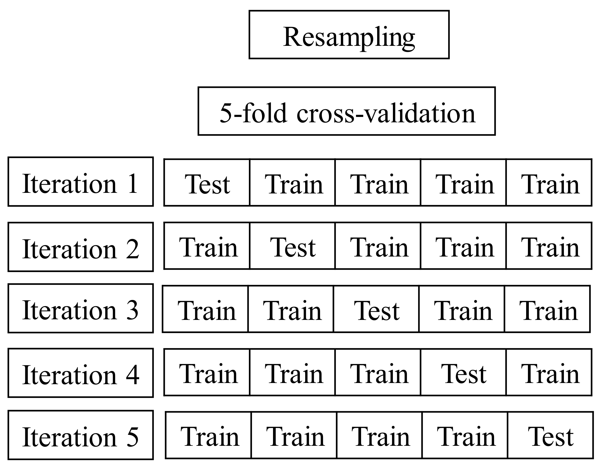
There are other resampling methods, for example, the validation set approach and leave-one-out cross-validation (LOOCV). On one hand, the validation set approach divides the training data only into two parts, causing the error rates to be very sensitive to the way the data is divided. On the other hand, LOOCV only leaves one observation for the test data so it is a very computationally intensive process although the error rates are very stable. Thus, K-fold cross-validation is the in-between method that handles the disadvantages of the other approaches; it provides relatively stable results, and it is computationally cheaper. For the value of K, in general, 5 and 10 are preferred since they both yield a relatively stable classification error rate. In this dissertation, five-fold cross-validation was mostly implemented because stepwise selection methods were taking a lot of time selecting the features and fitting the model with the ones before chosen. See Figure 2.

4. Empirical Analysis

4.1. Sample Data and Variables

The data were obtained from Chung Hua University in Taiwan. The data set contains 30,000 observations with 25 different columns, which are both categorical and numerical variables. The categorical variables give some qualitative characteristics about each client, such as gender, education, and marital status. On the other hand, the numerical variables represent the age of the clients, the amount of credit granted, the payment status, the number of bills, and the amount of payment for six months from April 2005 to September 2005. Lastly, the variable of interest illustrates the status of default of each customer in the following month; 1 for those who defaulted and 0 otherwise.

Table 2. The description of the database variables.

Variables	Description	Values
ID	ID of each client
LIMIT_BAL	Amount of the credit that each client has
SEX	Gender	1 = male, 2 = female
EDUCATION	Education	1 = graduate school, 2 = university, 3 = high school, 4 = others
MARRIAGE	Marital status	1 = married, 2 = single, 3 = others
AGE	Age
PAY_1	Repayment status in September, 2005	−1 = if paid in time, 1 = if delayed for one month, …, 9 = if delayed for nine months or more.
PAY_2	Repayment status in August, 2005	Same
PAY_3	Repayment status in July, 2005	Same
PAY_4	Repayment status in June, 2005	Same
PAY_5	Repayment status in May, 2005	Same
PAY_6	Repayment status in April, 2005	Same
BILL_AMT1	Amount of bill in September 2005
BILL_AMT2	Amount of bill in August, 2005
BILL_AMT3	Amount of bill in July, 2005
BILL_AMT4	Amount of bill in June, 2005
BILL_AMT5	Amount of bill in May, 2005
BILL_AMT6	Amount of bill in April, 2005
PAY_AMT1	Amount paid in September, 2005
PAY_AMT2	Amount paid in August, 2005
PAY_AMT3	Amount paid in July, 2005
PAY_AMT4	Amount paid in June, 2005
PAY_AMT5	Amount paid in May, 2005
PAY_AMT6	Amount paid in April, 2005
DEFAULT	Default status	1 = yes, 0 = no

Notes: the variables that represent amounts are expressed in Taiwanese dollars. The age variable is in years.

provides a detailed description of the data. An example of practical implementation of this data set for credit scoring can be found in [55].

4.2. The Determination of Model Parameters for the KNN-Algorithm

Before the feature selection process, the parameter “number of neighbors” for the KNN algorithm is determined. Depending on the K parameter, the performance of the algorithm can differ considerably; as discussed earlier, a small number of neighbors (K) makes the model overfit, leading the test error rate to be large and the model tends to perform poorly with a large K. Therefore, it is important to have an appropriate value of K so that the classifier has the lowest test error rate. According to [56], in general, the parameter is chosen empirically by trying different numbers of neighbors so for this study as well, a range of values of K was tried for each feature selection method to find one with which the KNN had the lowest classification error rate.

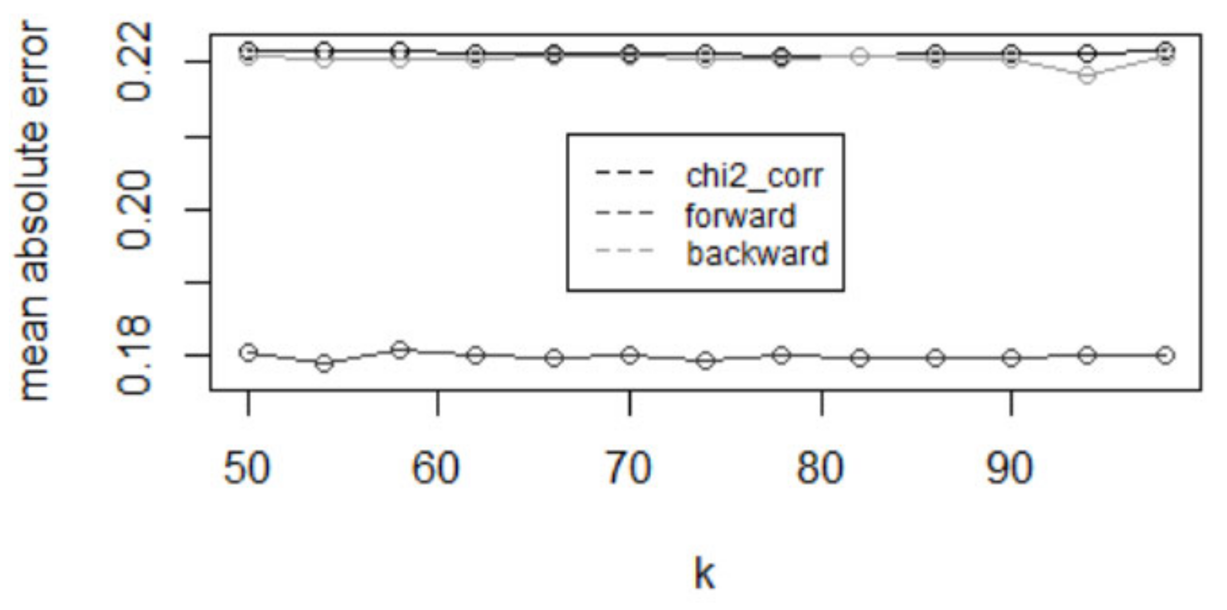
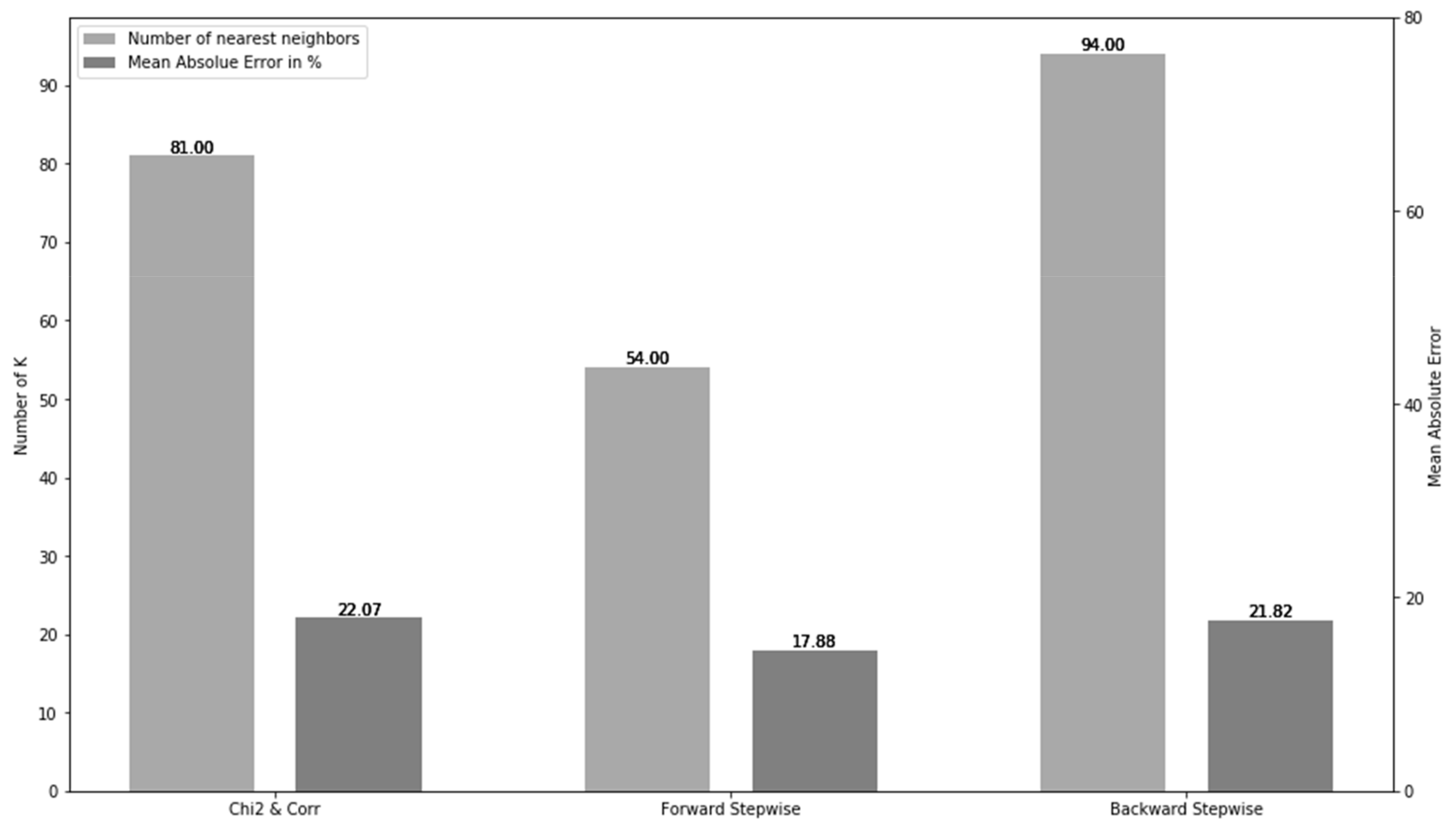
Figure 3 shows the changes in mean absolute error (MAE) as the classification error rate with different K_s when different feature selection methods were used in the KNN model. The range of K_s tried here was from 50 to 100 because there were too many possible values (from 0 to 30,000) to be considered so it was too computationally intensive to try all those values. According to Figure 4, the Chi-squared test and correlation coefficient provide the value of K as 81 with the lowest MAE of 22.07 percent. Regarding the other methods, the forward stepwise selection method required the KNN to consider 54 nearest neighbors for each test data observation for classification so that the algorithm has the lowest MAE of 17.88 percent. Lastly, backward stepwise selection provided the optimal K_s of 94 that yielded an MAE of 21.82 percent.

4.3. Empirical Results and Discussion

The classification algorithms were trained with the selected features. Then, two performance measures, model simplicity (the number of selected features) and model accuracy (the MAE) were used to see the effects of feature selection by comparing the performance measures before and after the selection process. Measuring the performance with the mean absolute error, although having some disadvantages, simplifies the considerations. Additionally, stepwise selection has two primary faults. On the one hand, false-positive findings. In this case, the corresponding p-values are unadjusted, leading to an over-selection of features (i.e., false-positive findings). This problem is exacerbated when highly correlated predictors are present. On the other hand, model overfitting: the resulting statistics are highly optimistic since they do not consider the selection process, so we have used the two performance measures that reinforce each other, the number of selected features and the MAE.

Before anything else, the performances of the models without feature selection are shown in

Table 3. Models without feature selection.

Models	No. of Features	Mean Absolute Error (%)
Logistic regression	24	22.120
KNN (K = 73)	24	22.057
SVM	24	22.120
Random forests	24	25.267

. The models without feature selection used all the features for fitting so they scored the same model simplicity (no change in the number of selected features). When it comes to MAEs without feature selection, however, we could detect gaps among the classifiers; the random forest classifier was the one that registered the highest MAE rate of 25.27 percent, meaning that it had the worst model accuracy. The other classifiers had similar error rates but the KNN with K equal to 73 yielded the lowest rate of 22.06 percent.

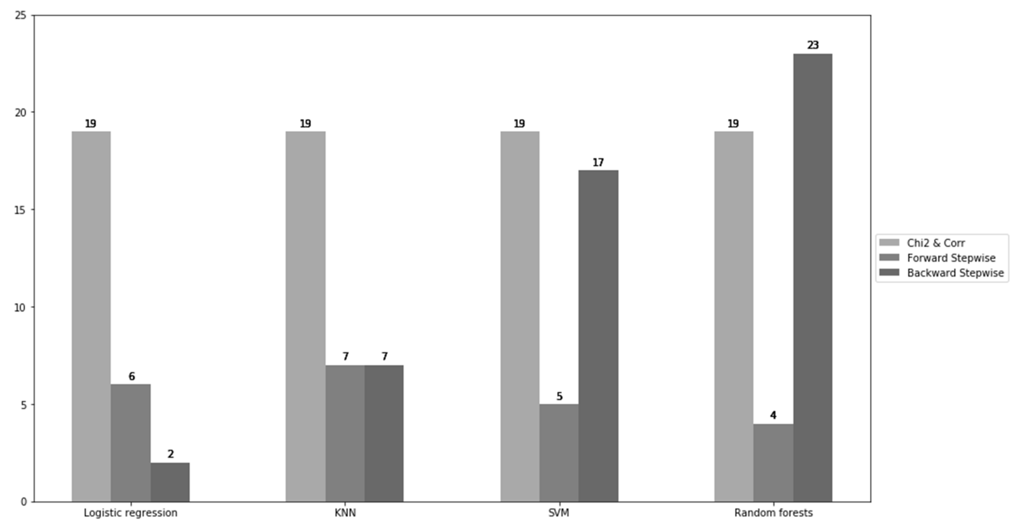
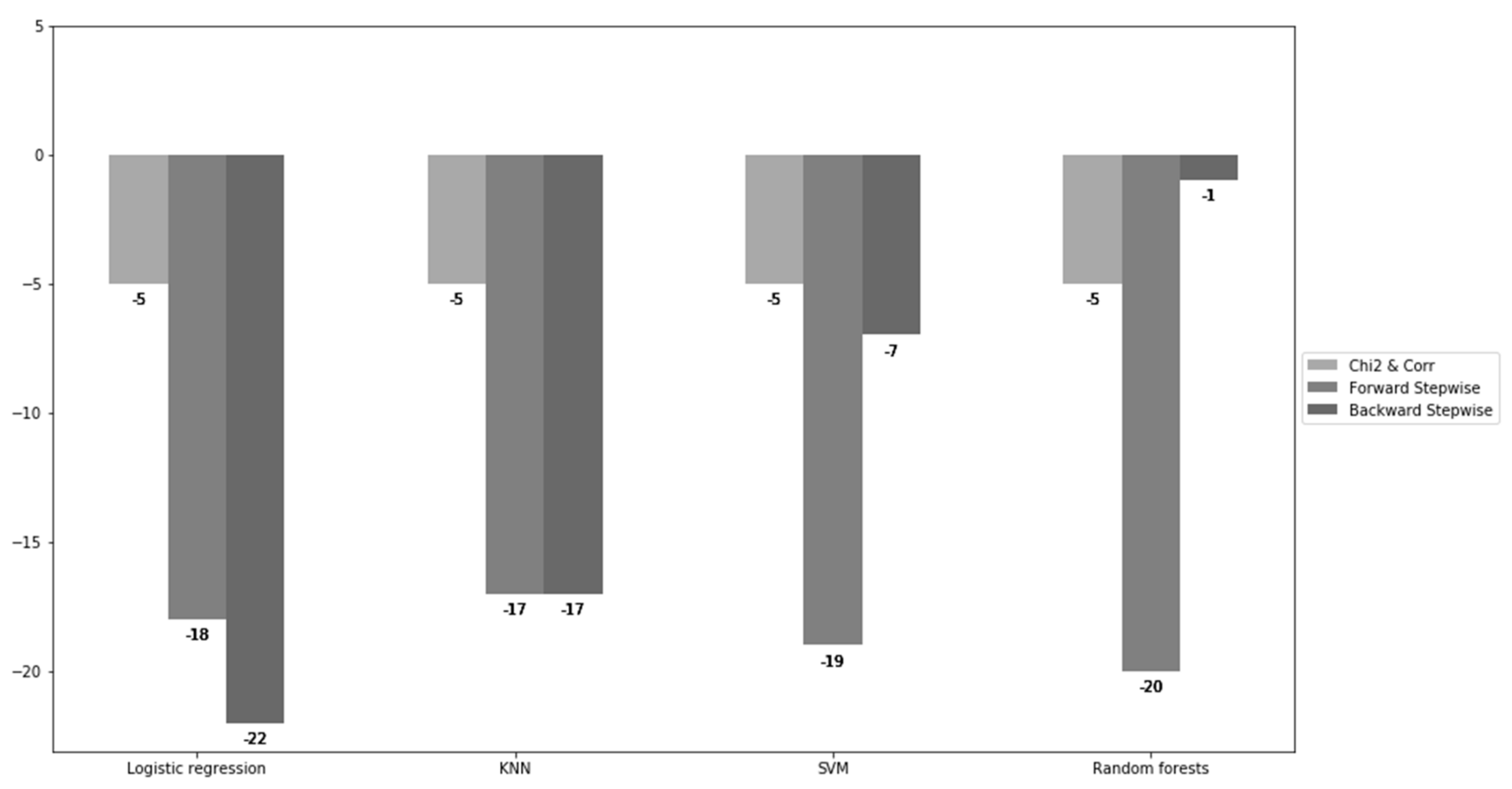
Figure 5 and Figure 6 illustrate the number of selected features for each of the classification algorithms using feature selection methods and the changes in model simplicity after it. The models with all 24 features are used as the criterion for the comparison. The most significant reduction in the number of features was made in the logistic regression, and only two features were chosen by the backward stepwise selection method, and six features by the forward stepwise selection. The reduction was also comparable for the KNN classifier as both forward and backward stepwise selection methods selected seven features. For SVM and random forest, the forward stepwise selection method helped to achieve a substantial decrease in features (five and four, respectively), whereas the features by the backward stepwise selection method only reduced by seven and one, respectively.

Table 4. The features selected by the Chi-squared test and correlation coefficient.

Models/Feature Selection	Chi2 and Corr
Logistic regression	(‘SEX’, ‘MARRIAGE’, ‘EDUCATION’, ‘LIMIT_BAL’, ‘PAY_1’, ‘PAY_2’, ‘PAY_3’, ‘PAY_4’, ‘PAY_5’, ‘PAY_6’, ‘BILL_AMT1’, ‘BILL_AMT3’, ‘PAY_AMT1’, ‘PAY_AMT2’, ‘PAY_AMT3’, ‘PAY_AMT4’, ‘PAY_AMT5’, ‘PAY_AMT6’)
KNN	Same
SVM	Same
Random forests	Same

provides the features or variables selected by the Chi-squared test and correlation coefficient method for the different models used.

Table 5. The features selected by forward stepwise method.

Models/Feature Selection	Forward Stepwise Selection
Logistic regression	(‘SEX’, ‘EDUCATION’, ‘AGE’, ‘PAY_1’, ‘PAY_5’, ‘PAY_6’)
KNN	(‘SEX’, ‘EDUCATION’, ‘MARRIAGE’, ‘PAY_1’, ‘PAY_3’, ‘PAY_5’, ‘PAY_6’)
SVM	(‘EDUCATION’, ‘PAY_1’, ‘PAY_4’, ‘PAY_5’, ‘PAY_6’)
Random forests	(‘EDUCATION’, ‘MARRIAGE’, ‘PAY_1’, ‘PAY_2’)

and

Table 6. The features selected by backward stepwise selection.

Models/Feature Selection	Backward Stepwise Selection
Logistic regression	(‘SEX’, ‘PAY_1’)
KNN	(‘BILL_AMT3’, ‘BILL_AMT6’, ‘PAY_AMT1’, ‘PAY_AMT2’, ‘PAY_AMT3’, ‘PAY_AMT4’, ‘PAY_AMT5’)
SVM	(‘SEX’, ‘EDUCATION’, ‘MARRIAGE’, ‘AGE’, ‘PAY_1’, ‘PAY_2’, ‘PAY_3’, ‘PAY_4’, ‘PAY_5’, ‘PAY_6’, ‘BILL_AMT1’, ‘BILL_AMT2’, ‘BILL_AMT3’, ‘BILL_AMT4’, ‘BILL_AMT6’, ‘PAY_AMT1’)
Random forests	(‘LIMIT_BAL’, ‘SEX’, ‘EDUCATION’, ‘MARRIAGE’, ‘AGE’, ‘PAY_1’, ‘PAY_2’, ‘PAY_3’, ‘PAY_5’, ‘PAY_6’, ‘BILL_AMT1’, ‘BILL_AMT2’, ‘BILL_AMT3’, ‘BILL_AMT4’, ‘BILL_AMT5’, ‘BILL_AMT6’, ‘PAY_AMT1’, ‘PAY_AMT2’, ‘PAY_AMT3’, ‘PAY_AMT4’, ‘PAY_AMT5’, ‘PAY_AMT6’)

show the features selected by forward and backward stepwise selection methods, respectively, for the different classification algorithms.

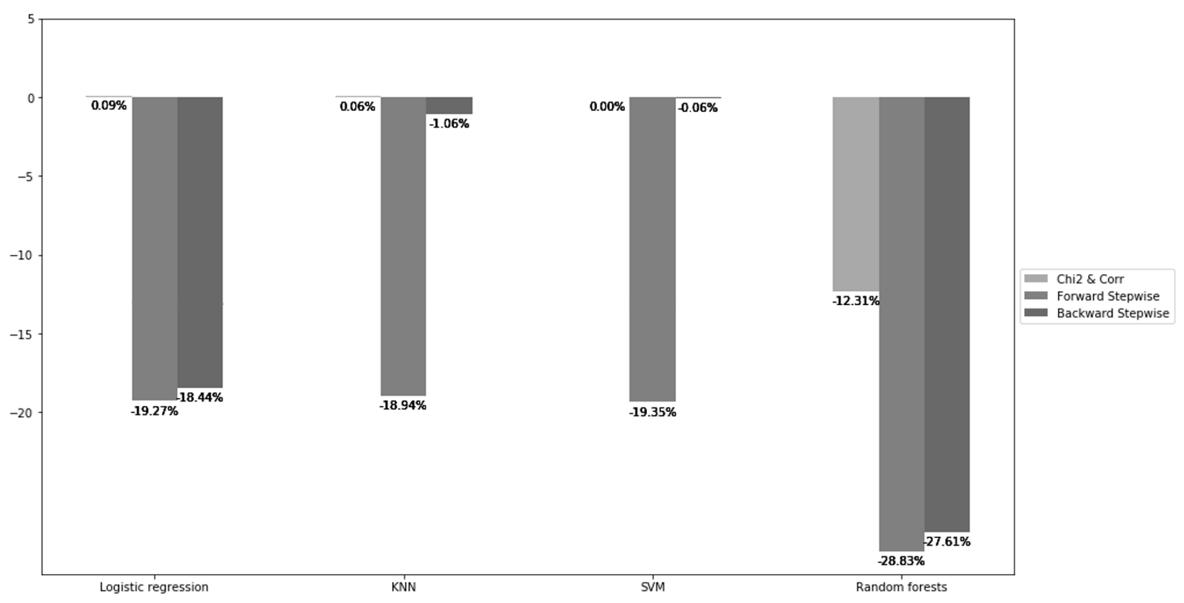
The changes in model accuracy are shown in Figure 7. The random forest showed the largest improvement in MAE after feature selection, even if there was not much reduction in the number of selected features, compared to the other models as mentioned earlier. Next, the logistic regression could be able to perform better by on average 12.6% and most of the improvement came from the forward and backward stepwise selection methods. On the contrary, for the KNN and SVM, it is clearly seen that the Chi-squared and correlation coefficient test and backward stepwise selection were not very helpful for the models to cut down MAE as the changes were close to 0.

Among the three feature selection methods, the forward stepwise selection method performed relatively superior to the other two methods concerning model simplicity and model accuracy. As we can see in

Table 7. The comparison of the results across all the experiments.

Models/Feature Selection	Chi2 and Corr	Forward Stepwise	Backward Stepwise
Logistic regression	(1) −5 (2) +0.0904%	(1) −18 (2) −19.2736%	(1) −22 (2) −18.4449%
KNN	(1) −5 (2) 0.0603%	(1) −17 (2) −18.9362%	(1) −17 (2) −1.0577%
SVM	(1) −5 (2) 0%	(1) −19 (2) −19.3491%	(1) −7 (2) −0.0601%
Random forests	(1) −5 (2) −12.3084%	(1) −20 (2) −28.8259%	(1) −1 (2) −27.6121%

(1) Change in model simplicity (in the number of features), (2) change in model accuracy (+: increase, −: decrease, 0: no change).

, the classification algorithms using the forward stepwise selection were simpler, that is, the models had fewer features, which made them easier to be interpreted. Besides, the classifiers using this selection method obtained the greatest reduction in MAE rates.

In addition, the features selected seemed more relevant to the response variable (“DEFAULT”) than those selected by the other selection methods according to Table 3, Table 4 and Table 5. For example, all the classification algorithms generated by the Chi-squared test and correlation coefficient, and the SVM and random forest classifier by backward stepwise selection included an “ID” feature for generating the models. However, this feature, in context, only represents the id of the clients so it can be said that this variable does not have anything to do with the level of credit risk. That is why it is not included.

It is also shown that the Chi-squared test and correlation coefficient have an inferior performance compared to the others. Even if the number of selected features decreased by five, the changes in MAE were not very much significant. The MAE for the random forest classifier, for instance, decreased by more than around 12 percent but the improvement was relatively small in comparison with the cases when the other selection methods were used. This inferior performance might be due to the characteristic of the filter methods; since they do not need any predictive model for feature selection, the subset of chosen features is the same for all the classifiers so it is likely that the models cannot make the most use of the chosen subset of features.

More studies would have to be done in order to draw more generalized conclusions. Specifically, other real data sets for different countries would be needed to consolidate the conclusions obtained, and other feature selection methods and classification algorithms could be included for future research. It would also be interesting to study the impacts of the wrapper or embedded methods after using filter methods as the preliminary step. Additionally, there are other important factors other than the MAE and the number of selected features when choosing a model in practice, such as the change in time of training models. However, it could be surely said that the data mining feature selection method is a great tool for picking out the most significant features from many through which it could become the key to effective credit scoring models.

4.3.1. Comparison of Findings with Existing Literature—Managerial Implications

The results obtained in this study suggest that the feature selection process helped credit scoring models to be simpler, making them more understandable and having lower classification error rates as measured in MAE. These merits might provide some of the reasons to carry out necessary feature selection processes in financial institutions. Ben David and Frank [57] concluded that for classification problems, machine learning models do not surpass hand-crafted models when prediction accuracy is considered most times. However, most of the studies comparing the predictive power of credit scoring models based on machine learning techniques with that of traditional loss and default models concluded the models using machine learning were better at predicting losses and defaults [17,58]. This performance would be further improved using feature selection methods.

From a managerial point of view, our results in addition to the huge machine learning literature base applied to credit scoring, reinforce the main conclusion that [4] obtained in their seminal paper, that is: improving a credit scoring model that detects applicants with bad credit, even by one percent, could lead to a significant decrease in the loss for financial institutions. Additionally, managers might be reluctant to implement advanced machine learning applications given that they require much expertise to handle. Ref. [7] addressed this issue by emphasizing that more accurate prediction could be achieved as the credit scoring models do not require any human intervention, creating a trend for managers to make decisions based on current data, thus convincing others to adopt these scoring methods more and more. Therefore, even if managers have to bear some costs of investing in sophisticated scoring methods, in the end, the investment will lead to a great pay-off when its benefits, such as saving time and effort or decreasing financial losses, accumulate over time.

4.3.2. Revisiting Credit Scoring Models: From Altman Z-Score to Machine Learning with Feature Selection Methods

Everyone in finance is familiar with the Altman Z-Score. Many analysts use it despite data not meeting their very restrictive assumptions. Altman (1968) applied a multivariate discriminant analysis (MDA) in connection with a prediction of bankruptcies, creating a model called the Z-score model. This method produces a score. An observation of the data is classified into a group, depending on the score relative to an arbitrary cut-off value. The method is based on the minimization of the variance among observations of the same group and the maximization of the distance between observations of different groups [59]. The restrictive assumptions of MDA, such as requiring normally distributed variables and sensitivity to outliers, could induce relevant mistakes if previously the analysis about bankruptcy did not try to test if the used data filled these assumptions [60,61,62,63]. Therefore, researchers and practitioners have sought to improve bankruptcy-forecasting models using alternative quantitative approaches.

Logistic regression (LR) was the first candidate as a multivariate model for application scoring and, subsequently, for credit risks modeling [64]. Not only are the assumptions less restrictive, but LR also produces a result in the [0, 1] interval that can be interpreted as the probability of a given observation being a member of a specific group [65]. Nevertheless, since credit risk analysis is similar to pattern-recognition problems, algorithms began to be used to classify the creditworthiness of counterparties [66,67], improving traditional models based on simpler multivariate statistical techniques such as discriminate analysis and logistic regression. This favored the use and extension of machine learning techniques in bankruptcy analysis because they assess patterns in observations of the same classification and identify features that differentiate the observations of different groups. In Section 2.2 we review the literature of machine learning and credit scoring, including support vector machine, K-nearest neighbors (KNN), and random forest as used in this work.

Table 8. Advantages and disadvantages of credit scoring models: form Altman Z-score to machine learning with feature selection methods.

Models	Advantages	Disadvantages
Multivariate Discriminant Analysis	(1) First model to predict bankruptcy (2) Simplicity: easy to interpret	(1) Required normally distributed variables (2) Sensitivity to outliers (3) It does not include nonlinearities (4) It does not offer a non-parametric approach
Logistic Regression	(1) Assumptions are less restrictive (2) It produces a [0, 1] interval result that can be interpreted as a probability of a given observation being a member of a specific group (3) Good interpretability and simple explanation	(1) Assumes a logistic regression: it is limited to additive form of the model (2) Assumes linearity in the covariances (3) It does not include nonlinearities (4) It does not offer a non-parametric approach
Machine Learning without Features Selection	(1) Credit risk analysis is similar to pattern recognition problems (2) It improves traditional models based on a simple multivariate statistical technique (3) It includes nonlinearities (4) It offers non-parametric approaches	(1) Sometimes complex models harder to interpret (2) High variance and overfitting in the curse of dimensionality (3) Excessive variety of possible models and combined techniques
Machine Learning with Features Selection	(1) Credit risk analysis is similar to pattern recognition problems (2) It improves traditional models based on a simple multivariate statistical technique (3) It includes nonlinearities (4) It offers non-parametric approaches (5) Simpler models easy to interpret (6) No overfitting	(1) Excessive variety of possible models and combined techniques

shows the general advantages and disadvantages of the revisiting of credit scoring models from Altman Z-score to Machine Learning with Feature Selection Methods.

This paper has presented a methodology for the selection of the key variables in order to establish a credit scoring. Logistic regression, support vector machine, K-nearest neighbors (KNN), and random forest are proposed in order to separate data into two classes and identify which candidates are likely to default for this credit scoring. Furthermore, this work has introduced an additional step, the use of three different feature selection methods in order to mitigate the overfitting in the curse of dimensionality of these classification algorithms. The performances of these three methods are discussed using two measures, the mean absolute error and the number of selected features. Our results suggest that forward stepwise selection yields superior performance in each of the classification algorithms used. Although the final model performance will depend on the specific characteristics of the classification problem and on the data structure [68], our results pointed out that the feature selection process helped credit scoring models to be simpler, making them more understandable and to have lower classification error rates as measured in MAE. Therefore, as an important conclusion, financial institutions in credit risk analysis necessarily must incorporate feature selection processes.

In summary, from the seminal Altman Z-Score model and the use of multivariate statistical techniques, such as discriminate analysis and logistic regression to assess credit risk, academics and practitioners, amid advances in computer technology, began to explore and use artificial intelligence and machine learning tools to classify the creditworthiness of counterparties. Moreover, different feature selection methods have been incorporated in order to mitigate the overfitting in the curse of dimensionality of these classification algorithms. The progress that has been made in credit risk analysis has been impressive, and even though it should be further investigated, questions about which tools and theories are most appropriate for such analyses are beginning to close.

4.3.3. Limitations and Future Research

The main goal of our methodology was to get a robust but easy to implement approach about the default ability of the risks in a portfolio. It is worth highlighting the existing alternatives in the different phases of our methodology, summarized in Figure 1, for future research. The aim would be to determine which tools, in the different phases, are the most appropriate regarding credit risk analysis. Therefore, in this section, future lines of research are detailed.

First, this paper classifies borrowers into two categories. It is just a simplified assumption. In future research, the aim will be to classify borrowers into more rating categories. Second, most studies on credit scoring rely on a single performance measure or measures of the same type. In general, performance measures were split into three types. Those that assess the discriminatory ability of the scorecard, those that assess the accuracy of the scorecard’s probability predictions, and those that assess the correctness of the scorecard’s categorical predictions [7]. Different types of indicators embody a different notion of classifier performance. Few studies mix evaluation measures from different categories. This paper uses MAE, which is one of the most common accurate measures. However, there are other discrimination measures in credit scoring, such as the area under the receiver operating characteristics curve (AUC), H-measure, pairwise comparison (e.g., paired t-test), analysis of variance, Friedman test, or Friedman test together with post-hoc test, Press’s Q statistic, and Cohen’s Kappa statistic [7,57]. Future research should include mixed evaluation measures from different categories.

Stepwise selection has two primary faults. On the one hand, false-positive findings. In this case, the corresponding p-values are unadjusted, leading to an over-selection of features. This problem is exacerbated when highly correlated predictors are present. On the other hand, model overfitting: the resulting statistics are highly optimistic since they do not consider the selection process. So, we have used two performance measures that reinforce each other, model simplicity (the number of selected features) and model accuracy (the MAE). In future research, we will include a threshold statistic, a p-value testing improvement, in order to measure the model quality.

In addition, some of the used classification algorithms will be expanded. For instance, it should use in addition to K-nearest neighbors, other more advanced methods such as Kernel K-Means. The same respect SVM method, including a multi-kernel SVM, or the kernel family (nested kernels, hierarchical kernels, mixture kernels, or ARD kernels). Finally, other real data sets for different countries would be needed to consolidate the conclusions obtained, including longer time windows.

Table 9. Benefits and future lines of research methodology proposed.

Benefits	Future Lines of Research
(1) Main concern is the practical use of models (2) Designed research is clear (3) Different classification algorithms are used (4) Performance measures used, model simplicity (number of selected features), and model accuracy (MAE) avoid false-positive findings, over-selection of features and model overfitting (5) Either the attributes selected or the number of them is indicated	(1) Combined techniques (2) Include change and/or growth variables. (3) Comparison with other performance measures (4) Classify borrowers in more than two variables (5) Other real data set for other countries would be needed

sums-up the benefits of our methodology and future lines of research.

5. Conclusions and Discussion

The restrictive assumptions of Altman Z-Score multivariate discriminant analysis (MDA) prompted researchers and practitioners to improve bankruptcy-forecasting models using alternative quantitative approaches. Since credit risk analysis is similar to pattern-recognition problems, algorithms began to be used to classify the creditworthiness of counterparties [65,66], improving traditional models based on simpler multivariate statistical techniques such as discriminate analysis and logistic regression. That favored the use and extension of machine learning techniques in bankruptcy analysis because they assess patterns in observations of the same classification and identify features that differentiate the observations of different groups.

This work is a research paper based on a review of the literature of machine learning and credit scoring, including support vector machine, K-nearest neighbors (KNN), and random forest used in this work. Logistic regression, support vector machine, K-nearest neighbors (KNN), and random forest were proposed in order to separate data into two classes and identify which candidates were likely to default for this credit scoring. Furthermore, this work has introduced an additional step, the use of three different feature selection methods in order to mitigate the overfitting in the curse of dimensionality of these classification algorithms. Therefore, there is a review of the feature selection methods used in the literature to reduce the curse of dimensionality. In this context, we introduce and develop a methodology for the selection of the key variables in order to establish a credit scoring, presented in Figure 1. Therefore, above all, this is a research paper.

The primary activity of commercial banks and other financial institutions is the granting of loans and credits to households and businesses. That is why analyzing the credit risk and trying to avoid defaults on loans and credits granted has become a key task of the financial institutions’ risk department. One of the most widely used techniques is credit scoring models. However, reality has demonstrated in different economic and financial crises, the latest example being the subprime crisis of 2008, the huge problems that the design and implementation of these credit scoring models present when it comes to identifying ex ante which candidates are likely to end up in default.

The growing availability of an enormous amount of data by financial institutions on their customers and the rapid development of artificial intelligence has allowed the use of classification algorithms and automatic learning techniques with the aim of separating and classifying these customers, identifying those who may default. However, the application of artificial intelligence presents several statistical problems, from the stability of the estimations as the sample size increases to the curse of dimensionality. The latter happens when data space grows at a very rapid speed as the number of dimensions, or features, grows. The predictive power of a classifier or a regressor increases with the number of features but decreases after the number reaches a critical point. Considering an excessive number of features could also cause other problems than reducing the performance of the model. Models with many features tend to be complex, which makes them harder to interpret than models with a small number of predictors. The sophisticated models also require more time for fitting data, and they tend to have a higher variance; in other words, they tend to overfit. Overfitting occurs when a machine-learning algorithm fits too close to the training data set but performs poorly on the test data set. However, there are ways to alleviate this curse by reducing the number of features when the size of data is relatively small. In the academic research, we can find different feature selection methods that allow picking a subset of features based on different evaluation metrics, the most relevant being the wrapper, filter, and embedded methods.

This paper presents a methodology for the selection of the key variables in order to establish a credit scoring. Different classification algorithms—logistic regression, support vector machine, K-nearest neighbors (KNN), and random forest—are proposed in order to separate data into two classes and identify which candidates are likely to default for this credit scoring. Three different feature selection methods are used in order to mitigate the overfitting in the curse of dimensionality of these classification algorithms, specifically one filter method (Chi-squared test and correlation coefficients) and two wrapper methods (forward stepwise selection and backward stepwise selection). The performances of these three methods are discussed using two measures, the mean absolute error and the number of selected features. The methodology is applied for a valuable database of Taiwan obtained from Chung Hua University. The results suggest that forward stepwise selection yields superior performance in each one of the classification algorithms used. The feature selection process helped credit-scoring models to be simpler making them more understandable, and having lower classification error rates as measured in MAE. These merits might give some of the reasons to carry out the feature selection process necessarily by financial institutions.

The classification algorithms and feature selection methods used in the paper are well-known and widely used. However, the main novelty and advantage of our methodology was to get a robust but easy to implement approach about the default ability of the risks in a portfolio. Stepwise selection has two primary faults. On one hand, false-positive findings. In this case, the corresponding p-values are unadjusted, leading to an over-selection of features. This problem is exacerbated when highly correlated predictors are present. On the other hand, model overfitting: the resulting statistics are highly optimistic since they do not consider the selection process; given this, we have used two performance measures that reinforce each other: model simplicity (the number of selected features), and model accuracy (the MAE). Both of them avoid these problems.

Future research would have to be done in order to draw more generalized conclusions. Specifically, other real data sets for different countries would be needed to consolidate the conclusions obtained, and other feature selection methods and classification algorithms could be included. It would also be interesting to study the impacts of the wrapper or embedded methods after using filter methods as the preliminary step. In addition, apart from the MAE and the number of features selected when choosing a model in practice, other factors can be used such as the change in time of the training models. Finally, the goal of scoring models will not be to classify borrowers only into two categories but commonly into more rating categories. Surely, what must be clear is that the data mining feature selection method is a great tool for picking out the most significant features from many, through which it could become the key to effective credit scoring models.

References

- Jacobson, T.; Roszbach, K. Bank lending policy, credit scoring and value-at-risk. J. Bank. Financ. 2003, 27, 615–633. [Google Scholar] [CrossRef] [Green Version]
- Saunders, A.; Cornett, M.M. Financial Institutions Management: A Risk Management Approach; McGraw-Hill Education: New York, NY, USA, 2017; pp. 1–912. [Google Scholar]
- Ong, C.-S.; Huang, J.-J.; Tzeng, G.-H. Building credit scoring models using genetic programming. Expert Syst. Appl. 2005, 29, 41–47. [Google Scholar] [CrossRef]
- Hand, D.J.; Henley, W.E. Statistical Classification Methods in Consumer Credit Scoring: A Review. J. R. Stat. Soc. Ser. A Stat. Soc. 1997, 160, 523–541. [Google Scholar] [CrossRef]
- Alpaydin, E. Introduction to Machine Learning, 2nd ed.; The MIT Press: Cambridge, MA, USA, 2010; pp. 1–579. [Google Scholar]
- Abellán, J.; Castellano, J.G. A comparative study on base classifiers in ensemble methods for credit scoring. Expert Syst. Appl. 2017, 73, 1–10. [Google Scholar] [CrossRef]
- Lessmann, S.; Baesens, B.; Seow, H.-V.; Thomas, L.C. Benchmarking state-of-the-art classification algorithms for credit scoring: An update of research. Eur. J. Oper. Res. 2015, 247, 124–136. [Google Scholar] [CrossRef] [Green Version]
- Baesens, B.; Van Gestel, T.; Viaene, S.; Stepanova, M.; Suykens, J.; Vanthienen, J. Benchmarking state-of-the-art classification algorithms for credit scoring. J. Oper. Res. Soc. 2003, 54, 627–635. [Google Scholar] [CrossRef]
- Garcia, V.; Marqués, A.I.; Sánchez, J.S.; Garreta, J.S.S. Non-parametric Statistical Analysis of Machine Learning Methods for Credit Scoring. Adv. Intell. Syst. Comput. 2012, 171, 263–272. [Google Scholar] [CrossRef]
- Hung, C.; Chen, J.-H. A selective ensemble based on expected probabilities for bankruptcy prediction. Expert Syst. Appl. 2009, 36, 5297–5303. [Google Scholar] [CrossRef]
- Dastile, X.; Celik, T.; Potsane, M. Statistical and machine learning models in credit scoring: A systematic literature survey. Appl. Soft Comput. 2020, 91, 106263. [Google Scholar] [CrossRef]
- Liu, Y.; Schumann, M. Data mining feature selection for credit scoring models. J. Oper. Res. Soc. 2005, 56, 1099–1108. [Google Scholar] [CrossRef]
- Tripathi, D.; Edla, D.R.; Cheruku, R.; Kuppili, V. A novel hybrid credit scoring model based on ensemble feature selection and multilayer ensemble classification. Comput. Intell. 2019, 35, 371–394. [Google Scholar] [CrossRef]
- Zhang, W.; Yang, D.; Zhang, S.; Ablanedo-Rosas, J.H.; Wu, X.; Lou, Y. A novel multi-stage ensemble model with enhanced outlier adaptation for credit scoring. Expert Syst. Appl. 2021, 165, 113872. [Google Scholar] [CrossRef]
- Wang, T.; Qin, Z.; Zhang, S.; Zhang, C. Cost-sensitive classification with inadequate labeled data. Inf. Syst. 2012, 37, 508–516. [Google Scholar] [CrossRef]
- Kraus, A. Recent Methods from Statistics and Machine Learning for Credit Scoring. Ph.D. Thesis, Fakultät für Math-Ematik, Informatik und Statistik, Ludwig-Maximilians-Universit at Munchen, München, Germany, 2014. [Google Scholar]
- Munkhdalai, L.; Munkhdalai, T.; Namsrai, O.-E.; Lee, J.Y.; Ryu, K.H. An Empirical Comparison of Machine-Learning Methods on Bank Client Credit Assessments. Sustainability 2019, 11, 699. [Google Scholar] [CrossRef] [Green Version]
- Teles, G.; Rodrigues, J.J.P.C.; Saleem, K.; Kozlov, S.; Rabêlo, R.A.L. Machine learning and decision support system on credit scoring. Neural Comput. Appl. 2020, 32, 9809–9826. [Google Scholar] [CrossRef]
- Akkoç, S. An empirical comparison of conventional techniques, neural networks and the three stage hybrid Adaptive Neuro Fuzzy Inference System (ANFIS) model for credit scoring analysis: The case of Turkish credit card data. Eur. J. Oper. Res. 2012, 222, 168–178. [Google Scholar] [CrossRef]
- Lee, T.H.; Sung-Chang, J. Forecasting creditworthiness: Logistic vs. artificial neural network. J. Bus. Fore-Cast. Methods Syst. 2000, 18, 28–30. [Google Scholar]
- Nie, G.; Rowe, W.; Zhang, L.; Tian, Y.; Shi, Y. Credit card churn forecasting by logistic regression and decision tree. Expert Syst. Appl. 2011, 38, 15273–15285. [Google Scholar] [CrossRef]
- Srinivasan, V.; Kim, Y.H. Credit Granting: A Comparative Analysis of Classification Procedures. J. Financ. 1987, 42, 665–681. [Google Scholar] [CrossRef]
- Shin, K.-S.; Lee, T.S.; Kim, H.-J. An application of support vector machines in bankruptcy prediction model. Expert Syst. Appl. 2005, 28, 127–135. [Google Scholar] [CrossRef]
- Bellotti, T.; Crook, J. Support vector machines for credit scoring and discovery of significant features. Expert Syst. Appl. 2009, 36, 3302–3308. [Google Scholar] [CrossRef] [Green Version]
- Danenas, P.; Garsva, G.; Gudas, S. Credit Risk Evaluation Model Development Using Support Vector Based Classifiers. Procedia Comput. Sci. 2011, 4, 1699–1707. [Google Scholar] [CrossRef] [Green Version]
- Kim, H.S.; Sohn, S.Y. Support vector machines for default prediction of SMEs based on technology credit. Eur. J. Oper. Res. 2010, 201, 838–846. [Google Scholar] [CrossRef]
- Martens, D.; Baesens, B.; Van Gestel, T.; Vanthienen, J. Comprehensible credit scoring models using rule extraction from support vector machines. Eur. J. Oper. Res. 2007, 183, 1466–1476. [Google Scholar] [CrossRef]
- Camastra, F. A SVM-based cursive character recognizer. Pattern Recognit. 2007, 40, 3721–3727. [Google Scholar] [CrossRef]
- Lu, C.; Van Gestel, T.; Suykens, J.; Van Huffel, S.; Vergote, I.; Timmerman, D. Preoperative prediction of malignancy of ovarian tumors using least squares support vector machines. Artif. Intell. Med. 2003, 28, 281–306. [Google Scholar] [CrossRef]
- Akay, M.F. Support vector machines combined with feature selection for breast cancer diagnosis. Expert Syst. Appl. 2009, 36, 3240–3247. [Google Scholar] [CrossRef]
- Tay, F.E.; Cao, L. Application of support vector machines in financial time series forecasting. Omega 2001, 29, 309–317. [Google Scholar] [CrossRef]
- Kim, K.-J. Financial time series forecasting using support vector machines. Neurocomputing 2003, 55, 307–319. [Google Scholar] [CrossRef]
- Safavian, S.R.; Landgrebe, D. A survey of decision tree classifier methodology. IEEE Trans. Syst. Man Cybern. 1991, 21, 660–674. [Google Scholar] [CrossRef] [Green Version]
- Wang, G.; Hao, J.; Ma, J.; Jiang, H. A comparative assessment of ensemble learning for credit scoring. Expert Syst. Appl. 2011, 38, 223–230. [Google Scholar] [CrossRef]
- Zhang, S. Nearest neighbor selection for iteratively kNN imputation. J. Syst. Softw. 2012, 85, 2541–2552. [Google Scholar] [CrossRef]
- Zhu, X.; Li, X.; Zhang, S. Block-Row Sparse Multiview Multilabel Learning for Image Classification. IEEE Trans. Cybern. 2016, 46, 450–461. [Google Scholar] [CrossRef]
- Lall, U.; Sharma, A. A Nearest Neighbor Bootstrap for Resampling Hydrologic Time Series. Water Resour. Res. 1996, 32, 679–693. [Google Scholar] [CrossRef]
- Zhu, X.; Zhang, S.; Jin, Z.; Zhang, Z.; Xu, Z. Missing Value Estimation for Mixed-Attribute Data Sets. IEEE Trans. Knowl. Data Eng. 2011, 23, 110–121. [Google Scholar] [CrossRef]
- James, G.; Witten, D.; Hastie, T.; Tibshirani, R. An Introduction to Statistical Learning with Applications in R; Springer: Berlin/Heidelberg, Germany, 2013; pp. 995–1039. [Google Scholar]
- Frydman, H.; Altman, E.I.; Kao, D.-L. Introducing Recursive Partitioning for Financial Classification: The Case of Financial Distress. J. Financ. 1985, 40, 269–291. [Google Scholar] [CrossRef]
- Zhang, D.; Zhou, X.; Leung, S.C.; Zheng, J. Vertical bagging decision trees model for credit scoring. Expert Syst. Appl. 2010, 37, 7838–7843. [Google Scholar] [CrossRef]
- Zibanezhad, E.; Foroghi, D.; Monadjemi, A. Applying decision tree to predict bankruptcy. In Proceedings of the 2011 IEEE International Conference on Computer Science and Automation Engineering, CSAE, Shanghai, China, 10–12 June 2011; pp. 165–169. [Google Scholar] [CrossRef]
- Laborda, R.; Laborda, J. Can tree-structured classifiers add value to the investor? Financ. Res. Lett. 2017, 22, 211–226. [Google Scholar] [CrossRef]
- Hughes, G. On the mean accuracy of statistical pattern recognizers. IEEE Trans. Inf. Theory 1968, 14, 55–63. [Google Scholar] [CrossRef] [Green Version]
- Jarman, K.H. Beyond Basic Statistics: Tips, Tricks, and Techniques Every Data Analyst Should Know. In Beyond Basic Statistics: Tips, Tricks, and Techniques Every Data Analyst Should Know, 1st ed.; John Wiley & Sons: Hoboken, NJ, USA, 2015; pp. 1–190. [Google Scholar] [CrossRef]
- Famili, A.; Shen, W.-M.; Weber, R.; Simoudis, E. Data Preprocessing and Intelligent Data Analysis. Intell. Data Anal. 1997, 1, 3–23. [Google Scholar] [CrossRef] [Green Version]
- Bermingham, M.L.; Pongwong, R.; Spiliopoulou, A.; Hayward, C.; Rudan, I.; Campbell, H.; Wright, A.F.; Wilson, J.F.; Agakov, F.; Navarro, P.; et al. Application of high-dimensional feature selection: Evaluation for genomic prediction in man. Sci. Rep. 2015, 5, 10312. [Google Scholar] [CrossRef] [Green Version]
- Efron, B.; Hastie, T.; Johnstone, I.; Tibshirani, R.; Ishwaran, H.; Knight, K.; Loubes, J.M.; Massart, P.; Madigan, D.; Ridgeway, G.; et al. Least angle regression. Ann. Stat. 2004, 32, 407–499. [Google Scholar] [CrossRef] [Green Version]
- Smith, G. Step away from stepwise. J. Big Data 2018, 5, 32. [Google Scholar] [CrossRef]
- Kuhn, M.; Johnson, K. Applied Predictive Modelling; Springer: Berlin/Heidelberg, Germany, 2015; pp. 1–600. [Google Scholar]
- Pearson, K.X. On the criterion that a given system of deviations from the probable in the case of a correlated system of variables is such that it can be reasonably supposed to have arisen from random sampling. Lond. Edinb. Dublin Philos. Mag. J. Sci. 1900, 50, 157–175. [Google Scholar] [CrossRef] [Green Version]
- Belsley, D.A. A Guide to using the collinearity diagnostics. Comput. Sci. Econ. Manag. 1991, 4, 33–50. [Google Scholar] [CrossRef]
- Goldstein, M.; Chatterjee, S.; Price, B. Regression Analysis by Example. J. R. Stat. Soc. Ser. A Stat. Soc. 1979, 142, 512. [Google Scholar] [CrossRef]
- Tibshirani, R. Regression Shrinkage and Selection via the Lasso. J. R. Stat. Soc. Ser. B Stat. Methodol. 1996, 58, 267–288. [Google Scholar] [CrossRef]
- Yeh, I.-C.; Lien, C.-H. The comparisons of data mining techniques for the predictive accuracy of probability of default of credit card clients. Expert Syst. Appl. 2009, 36, 2473–2480. [Google Scholar] [CrossRef]
- Hassanat, A.B.; Abbadi, M.A.; Altarawneh, G.A.; Alhasanat, A.A. Optimal K parameter for KNN Classifier with square root. Int. J. Comput. Sci. Inf. Secur. 2014, 12, 33–39. [Google Scholar]
- Ben-David, A.; Frank, E. Accuracy of machine learning models versus “hand crafted” expert systems—A credit scoring case study. Expert Syst. Appl. 2009, 36, 5264–5271. [Google Scholar] [CrossRef]
- Gambacorta, L.; Huang, Y.; Qiu, H.; Wang, J. How do Machine Learning and Non-Traditional Data Affect Credit Scoring? New Evidence from a Chinese Fintech Firm. BIS Working Papers 834. Available online: https://www.bis.org/publ/work834.pdf (accessed on 30 November 2020).
- Altman, E.I. Financial Ratios, Discriminant Analysis and the Prediction of Corporate Bankruptcy. J. Financ. 1968, 23, 589–609. [Google Scholar] [CrossRef]
- Mahmoudi, N.; Duman, E. Detecting credit card fraud by Modified Fisher Discriminant Analysis. Expert Syst. Appl. 2015, 42, 2510–2516. [Google Scholar] [CrossRef]
- McLeay, S.; Omar, A. The Sensitivity of Prediction Models to the Non-Normality of Bounded and Unbounded Financial Ratios. Br. Account. Rev. 2000, 32, 213–230. [Google Scholar] [CrossRef]
- Shumway, T. Forecasting Bankruptcy More Accurately: A Simple Hazard Model. J. Bus. 2001, 74, 101–124. [Google Scholar] [CrossRef] [Green Version]
- Chava, S.; Jarrow, R.A. Bankruptcy Prediction with Industry Effects. Rev. Financ. 2004, 8, 537–569. [Google Scholar] [CrossRef]
- Campbell, J.Y.; Hilscher, J.; Szilagyi, J. In Search of Distress Risk. J. Financ. 2008, 63, 2899–2939. [Google Scholar] [CrossRef] [Green Version]
- De Menezes, F.S.; Liska, G.R.; Cirillo, M.A.; Vivanco, M.J. Data classification with binary response through the Boosting algorithm and logistic regression. Expert Syst. Appl. 2017, 69, 62–73. [Google Scholar] [CrossRef]
- Kruppa, J.; Schwarz, A.; Arminger, G.; Ziegler, A. Consumer credit risk: Individual probability estimates using machine learning. Expert Syst. Appl. 2013, 40, 5125–5131. [Google Scholar] [CrossRef]
- Pal, R.; Kupka, K.; Aneja, A.P.; Militky, J. Business health characterization: A hybrid regression and support vector machine analysis. Expert Syst. Appl. 2016, 49, 48–59. [Google Scholar] [CrossRef]
- Duéñez-Guzmán, E.A.; Vose, M.D. No Free Lunch and Benchmarks. Evol. Comput. 2013, 21, 293–312. [Google Scholar] [CrossRef]
Figure 1.
The methodology proposed for credit scoring: classification algorithms used (LR, SVM, KNN, RF) trained with different feature selection methods.
Figure 2.
The resampling method used: five-fold cross-validation.
Figure 3.
The selection of parameter K for the KNN classifier.
Figure 4.
The number of nearest neighbors and mean absolute error.
Figure 5.
The number of selected features.
Figure 6.
The change in the model simplicity (no. of features).
Figure 7.
The change in MAE after feature selection.