Employing Fuzzy Logic to Analyze the Structure of Complex Biological and Epidemic Spreading Models

Abstract

Complex networks constitute a new field of scientific research that is derived from the observation and analysis of real-world networks, for example, biological, computer and social ones. An important subset of complex networks is the biological, which deals with the numerical examination of connections/associations among different nodes, namely interfaces. These interfaces are evolutionary and physiological, where network epidemic models or even neural networks can be considered as representative examples. The investigation of the corresponding biological networks along with the study of human diseases has resulted in an examination of networks regarding medical supplies. This examination aims at a more profound understanding of concrete networks. Fuzzy logic is considered one of the most powerful mathematical tools for dealing with imprecision, uncertainties and partial truth. It was developed to consider partial truth values, between completely true and completely false, and aims to provide robust and low-cost solutions to real-world problems. In this manuscript, we introduce a fuzzy implementation of epidemic models regarding the Human Immunodeficiency Virus (HIV) spreading in a sample of needle drug individuals. Various fuzzy scenarios for a different number of users and different number of HIV test samples per year are analyzed in order for the samples used in the experiments to vary from case to case. To the best of our knowledge, analyzing HIV spreading with fuzzy-based simulation scenarios is a research topic that has not been particularly investigated in the literature. The simulation results of the considered scenarios demonstrate that the existence of fuzziness plays an important role in the model setup process as well as in analyzing the effects of the disease spread.

1. Introduction

Graphs are appropriate mathematical structures to represent and analyze complex networks, and graph theory is a field in mathematics that deals with the study of graphs [1]. Graph theory supports the visualization and analysis of complex network structures. The World Wide Web (WWW) and the human brain, as it is studied in medical informatics, are representative examples of complex networks [2]. The graph representation and analysis of complex networks have been extended in numerous areas, such as biology, computer science, epidemiology, mathematics, physics, sociology and telecommunications [3]. In terms of the human brain, a graph structure represents a network of connected nerve cells, where corresponding cells can make up on their own a network and their task is to cause and create biochemical reactions [4]. Complex networks, represented as graphs, allow researchers to analyze their structural and behavioral properties. The comprehensive knowledge of a complex network structure may contribute to the extraction of valuable information with the aim of further assessing and enhancing methodologies, tools, as well as the outcomes of shaped examinations. All of these reasons contribute to the motivation of the present work, which deals with analyzing the problem of HIV spreading in a sample of needle drug individuals.

In the relevant literature, the epidemic spreading problem has attracted high attention towards the awareness of the dynamic procedures that are generated in corresponding complex networks [5]. The authors of [6] review and present various solved and open problems in the development, analysis, and control of complex epidemic models. Moreover, a detailed review of the extensive research that has been conducted on epidemic procedures is presented in [7]. Another representative research in the same area is presented in [8], where the authors study infections spreading in complex heterogeneous networks based on a Systemic Inflammatory Response Syndrome (SIRS) epidemic model with birth and death rates. The SIRS epidemic model is utilized in clustered networks with the aim of analyzing the impact of the network community structure on the epidemic spreading and dynamics. Besides human epidemic spreading, an additional issue studied with the use of complex network models is related to the impact of different types of animal movements regarding the conditions for the spread of an infectious disease [9].

In a relevant survey [10], the authors review and unify theoretical methods regarding epidemic spreading, in terms of escalating the complexity of the equations used by various methods. In this survey, the authors analyze various methods, including the mean-field approach and various variations of the mean-field approach, such as the heterogeneous mean-field and the quench mean-field. Moreover, the authors examine methods that involve pairwise approximation, link percolation and dynamic message-passing. The authors of [11] introduce effective algorithms for implementing complex networks, which have concrete statistical properties that are non-homogeneous. The authors also suggest a pseudo-code for reproducing complex directed or undirected networks by performing simulations of human brain functions. Regarding sexually transmitted diseases, such as AIDS, the work presented in [12] focuses on the early transmission, the following dissemination, and finally, the establishment of the HIV-1 virus in a human population. The authors claim that the outcomes of their evolutionary analyses are capable of rebuilding the initial dynamics of the HIV-1 virus and, as a result, draw attention to the role of social changes and transport networks within the establishment of this virus in a human population.

Nowadays, within the field of biosciences, a number of levels regarding imprecision and uncertainty, particularly in epidemiological studies, are involved in disease diagnosis [13]. A single disease could affect numerous patients in various ways, and a single symptom may be indicative of various diseases. More importantly, the occurrence of some diseases in a patient may disrupt the expected symptom pattern of any of them. As a result, this may cause a tremendous amount of uncertainty and imprecision towards the interpretation of impact measures. Fuzzy set theory, since its beginning in 1965 [14] as an abstraction of dual rationale and/or classical set theory, has progressed to an effective scientific theory [15]. It contributes a strict scientific (or specifically mathematical) framework in which unclear conceptual phenomena can be absolutely and thoroughly considered [14,16]. Specifically, fuzzy set theory can also be viewed as a modeling language, which is efficient for circumstances where fuzzy criteria and imprecise phenomena are taken into consideration.

In the current work, we analyze the structure and advancement of complex networks by means of an extensive study regarding graph theory by presenting their fundamental types (initially presented in [17]). Concretely, an epidemic model, which is based on fuzzy logic and is expected to set up a relation among the viral load as well as the clinical evolution to Acquired Immunodeficiency Syndrome (AIDS) in HIV contaminated users, is proposed. It is worth mentioning that HIV can be transmitted in different ways, although sexual intercourse is considered the most common and widespread. Nevertheless, HIV can also be transmitted through blood transfusions, through HIV-infected women who transmit the virus to their babies before or during birth, or even later through breastfeeding. However, in the present study, a special way of transmitting the virus is used, that is, with use of syringes that drug users inject. The proposed model is based on the Erdös–Renyi model and simulates the spread of HIV in an isolated human population. Furthermore, we tried to incorporate the basic principles of random graphs in order to favor certain types of graphs. Although this paper focuses on the context of epidemics, the same model can be directly applied to many different spreading processes in complex networks.

The remainder of the work is structured in the following way: In Section 2, basic preliminaries, complex networks models and epidemic models are introduced. In Section 3, we discuss issues related to fuzzy epidemics, while Section 4 introduces the datasets for validating our framework. Additionally, Section 5 overlooks the experiments that were conducted in order to evaluate our work and claim our findings along with the results assembled. Section 6 concludes the work by focusing on conclusions and considers aspects related to future work. Finally, the notation of this work is summarized in

Table 1. Basic notation.

Symbol	Meaning
k	Node’s Degree
$p_k$	Degree Distribution
L	Average Shortest Path Length
b	Betweenness Node
T	Transitivity
C	Clustering Coefficient
$c_i$	Local Clustering Coefficient of Node i
r	Probability Distribution Function related to Fuzzy Logic Setting
$\mathbb{U}$	Universe of Discourse
F	Fuzzy Set
u	Support Value
${\mu }_F\left(u\right)$	Membership Function
x	Linguistic Variable
$T\left(x\right)$	The Set of Names of x
$M\left(x\right)$	Semantic Rule

.

2. Theoretical Framework

This section presents the basic preliminaries of current work along with an introduction to complex network models and epidemic models that are considered in biological networks.

2.1. Basic Definitions

A graph G presents the connections/associations among the data of a system, which comprises nodes N as well as edges E. Concretely, a graph comprises a collection of data objects, entitled nodes. A number of these items are related with links named edges [18,19]. Specifically, in the event that the edges are considered towards one direction, then at that point, the graph is regarded as a directed graph [20]; otherwise, the graph is regarded as an undirected graph. An undirected graph is a complete graph where all nodes are interconnected in pairs [18].

In numerous applications, each graph is assigned with a related numeric value, entitled weight. In this particular case, the edges constitute non-negative integers, and as a result, the graph can be regarded as a weighted graph. In order for the definitions to be correlated, this graph can be directed or undirected while the edge’s weight is regularly alluded to as the “cost” of an edge.

In addition, a path constitutes a coherence of nodes, which keep the status of each consecutive pair $(V_i,V_{i+1})$, i.e., a graph’s edge. Except for the inclusion of the corresponding nodes, the path involves the coherence of edges that associate these nodes. In a number of cases, paths with repeated nodes can also be considered; however, in most cases, paths with non-repeated nodes are preferred. Specifically, in cases where a non-simple path traverses a particular node, this fact is emphasized as it is referred to as a normal non-simple path [18].

An important aspect that can be derived from graph structure concerns the type of the graph edges; if it is known, a diversity of valuable metrics that depict the graph’s characteristics in a more detailed way can be computed. Specifically, the notion of centrality is utilized to identify the specific graph nodes that are considered critical [21]. There are a number of possible ways for defining the importance of a node, but the simplest measure of centrality in a network is to observe the number of edges that are associated with each vertex-node. This specific definition is referred to as the degree centrality.

In more detail, the node’s degree i in an undirected graph consisting of N nodes is denoted by $k_i$; assuming an adjacency matrix, this degree can be considered as the sum of the ith row of the adjacency matrix [20], as presented in the following Equation (1):

$$k_i=\sum _{j=1}^N{A}_{ij}$$

(1)

In network topology, three measures are considered as the most robust; namely, the degree distribution, the average path length and the clustering coefficient, which will be presented in the following paragraphs. Initially, one of the major properties in terms of a graph is the degree distribution, as discussed in [2]. The amount of nodes of the corresponding network maintaining a degree with a number equal to k is indicated with $p_k$ and is presented in Equation (2). The overall fraction of these values $p_k$ produces the degree distribution with the aim of plotting this distribution of a specific network as a function of degree k as follows:

$$p_k=\frac{\mathrm{number}\mathrm{of}\mathrm{nodes}\mathrm{with}\mathrm{degree}\mathrm{k}}{n}$$

(2)

Another feature that plays a vital part in terms of the graph’s dissemination, as well as transmission, is the shortest path. The shortest paths are of great importance in characterizing the internal structure of the graph [19]. Thus, the majority of length values of the shortest paths of a given graph G needs to be provided so that when considering a corresponding table A, the input $a_{ij}$ can be associated with its length between nodes i and j. An important aspect of the graph is its diameter, which is defined as the maximum value of $a_{ij}$.

A representative partition among a number of nodes in a concrete graph is identified with the use of the average length of the shortest paths, which is typically introduced as the typical path length. The average path length is considered a concept in network topology that is defined as the average number of steps along the shortest paths for all possible pairs of network nodes. It is a measure of the efficiency of information or mass transport on a network. As an example, one can consider the average number of clicks that will lead you from one website to another. It should not be confused with the diameter of the network, which is defined as the longest geodesic, i.e., the longest shortest path between any two nodes in the network. The average shortest path length L is characterized as the average of the geodetic lengths over all pairs of nodes as presented in Equation (3):

$$L=\frac{{\sum }_{i,j\in N}^{}{d}_{ij}}{{\sum }_{i,j\in N}^{}{p}_{ij}}$$

(3)

where $d_{ij}$ denotes the shortest distance between nodes i and j; if $i=j$ or j cannot be reached from i then $d_{ij}=0$. In addition, $p_{ij}$ denotes if there is a path between nodes i and j; if $i=j$ or if there is no path from i to j then $p_{ij}=0$ and if there is a path from i to j then $p_{ij}=1$. The value of the all-pairs shortest-path length of a particular graph is denoted by ${\sum }_{i,j\in N}{d}_{ij}$, whereas ${\sum }_{i,j\in N}{p}_{ij}$ constitutes the number of paths that exist in this graph. For a connected undirected graph, ${\sum }_{i,j\in N}{p}_{ij}=N(N-1)$ because paths exist between any pair of nodes [22].

The communication between two non-adjacent nodes depends on the other nodes that belong to each path and connect them. Consequently, we can obtain whether a given node can communicate with a non-neighboring one by measuring the geodetic number, also known as a betweenness node.

More importantly, a betweenness node $b_i$ of a node i, often typically referred as load, is computed from the following Equation (4):

$$b_i=\sum _{j,k\in N,j\ne k}^{}\frac{n_{jk}\left(i\right)}{n_{jk}}$$

(4)

where $n_{jk}$ constitutes the number of the paths that connect faster node j with node k, whereas $n_{jk}\left(i\right)$ is the number of paths that connect the same nodes with the detailed information traversing through node i via the shortest path [23].

Furthermore, betweenness is considered as a metric that can be further expanded so as to be applied to the graph’s edges. In this case, the definition is slightly alternated, and thus, the edge betweenness constitutes the quantity of shortest paths among the pairs of nodes traversing the corresponding edge [24].

The method of clustering, which is as well declared as transitivity, constitutes a representative feature of contact networks. As contact networks, one can consider the example of two people having a mutual friend [19]. This may be evaluated by determining the clustering T of a graph as a respective quantity of triplets; namely, the fraction of the three connected triads as in Equation (5) [2]. The factor 3 in the numerator accounts for the aspect that each triangle, consisting of three nodes, is actually contributing three times, which is the connected triads, and guarantees that $0\le T\le 1$, with $T=1$.

$$T=\frac{3\times \mathrm{number}\mathrm{of}\mathrm{triangles}\mathrm{in}\mathrm{G}}{\mathrm{number}\mathrm{of}\mathrm{connected}\mathrm{triples}\mathrm{of}\mathrm{vertices}\mathrm{in}\mathrm{G}}$$

(5)

Another option that can be regarded as a factor is the utilization of the clustering coefficient C of the corresponding graph [25]. That is, given a concrete node i, this metric is equal to the quantity $c_i$, which is the local clustering coefficient. This quantity expresses the probability of $a_{jm}$ to become equal to 1 for two connected nodes to node i, namely j and m. More importantly, the definition of the local clustering coefficient can be estimated as the fraction among the quantity of edges $e_i$ and the maximum feasible number of edges $\frac{k_i(k_i-1)}{2}$ in one graph, as follows in Equation (6) [26]:

$$c_i=\frac{2e_i}{k_i(k_i-1)}=\frac{{\sum }_{j,m}^{}{a}_{ij}{a}_{jm}{a}_{mi}}{k_i(k_i-1)}$$

(6)

In the following, the clustering coefficient of the graph can be computed as the average of value $c_i$ for the entire number of nodes of the graph, as in Equation (7). By default, $0\le c_i\le 1$, as well as $0\le C\le 1$.

$$C=〈c〉=\frac{1}{N}\sum _{i\in N}^{}{c}_i$$

(7)

2.2. Models of Complex Networks

The structure and the characteristics of complex networks can be analyzed and understood by rigorously examining their corresponding modeling. Specifically, some major issues associated with the analysis and prediction of process behavior in the following simulation are found in the information retrieval, propagation and transmission.

2.2.1. Erdös–Renyi Model

The Erdös–Renyi [27] model is considered among the initial network models with the characteristic that it corresponds to the random graph. Concretely, regarding the model of a random graph, two major aspects of the nodes are represented, namely their quantity as well as the probability that two arbitrarily selected nodes are associated. For every pair of nodes, an equal probability is associated, which is independent of the remaining pairs, as stated in [20,27].

One of the critical reasons for which the Erdös–Renyi model has been widely acceptable is its attributes that encourage the process of modeling the network. Moreover, a special category of graphs, namely random graphs, does not efficiently correspond to the structure of real networks, since the majority of the node degrees in terms of this graph category results from the power-law distribution (Retrieved 27 April 2021, from https://necsi.edu/power-law) [28] rather than from Poisson distribution. In this way, the Erdös–Renyi model does not take into account the impact of the clustering process, while a random graph can be considered as an ideal model option for investigating complex networks [27].

2.2.2. Barabási–Albert Model

The most popular model, having degree distribution in power-law edges, is the Barabási–Albert model [29]. Concretely, the corresponding graphs are constructed under a dynamic process where the edges are added one by one to a core. The probability of a new edge to be linked with an existing one is proportional to the degree of the latter. According to the above, the edges with a high degree of distribution are more likely to be selected as adjacent to the new edges. Once this occurs, the degree of all edges will be increased so that there are more possibilities to be chosen in the future. This process creates a graph with a degree distribution that is characterized by a power-law tail as the number of edges tends to infinity.

The Barabási–Albert model presents a very small average-shortest-path length of a random graph as well as a clustering coefficient. This coefficient decreases with the size of the network and is lower than in real networks. The representation of the community structure of the actual complex networks is properly introduced in Figure 1.

2.3. Epidemic Models in Biological Networks

As a second category of complex networks, biological neural networks of living organisms along with their epidemic networks, are considered. More specifically, two main types of biological networks exist. In addition, we propose a reference to networks based on the heritage/legacy of individuals by utilizing the genetic material (deoxyribonucleic acid—DNA) in conjunction with common attributes that these corresponding individuals come up with from their predecessors. Additionally, the epidemic activity of complex networks utilized by the nodes sensitivity is presented. Furthermore, different scenarios are investigated, like the transferable filial diseases (airborne or sexually transmitted) among humans, which is propagated through different categories of networks, like complex internet ones, or social networks, or even among computers.

This category of networks is also similar to biological networks in terms of utilizing networking either among communities in living organisms or among organism functions. For example, the ecosystem, subsections, and nervous system of the brain, which is perhaps the most studied by scientists.

3. Fuzzy Epidemics

Biological pathogens, such as influenza, measles, as well as sexually transmitted diseases, can result in infectious and contaminating diseases, especially in cases where epidemic diseases are considered. These diseases have the major characteristic of transmitting among individuals. Epidemics are capable of massively contaminating the population or can be dormant for a long time without any evidence of their presence. In extraordinary cases, one unique disease outburst can have a considerable and critical impact on a whole culture; for example, one can consider the entity of epidemics activated by the entry of Europeans in America or even the deadly epidemic of smallpox as featured by the British during the 15th century.

3.1. Transmitted Diseases in Networks

An infectious disease can be spread among individuals within a population of a complex network, as thoroughly displayed in [30]. The network of contacts can lead to the spread and expansion of a corresponding contamination. If these individuals physically encounter each other, then they are likely to catch the disease. Therefore, the precision of the model in terms of the inherent network is of major importance in order to identify the epidemic spreading. A number of comparable works constitute the research of malware spread among computers [31].

3.2. Branching Processes

The branching process is considered as the elementary model of disease propagation, especially with respect to an airborne illness. These kinds of networks are often mentioned as trees, as presented in Figure 2. Transmission waves utilize the specific tree model by taking into consideration the following information: when a number of infections get involved in a healthy population by a group of individuals, at that point there exists a plausibility for the disease to be transmitted to a sensitive portion of this populace, in accordance with a random transmission possibility of the disease [18].

3.3. Susceptible–Infectious–Susceptible Model (SIS)

A basic variation regarding the epidemic models permits the hypothesis that people influenced by an epidemic can be infected a number of times. This characteristic epidemic model is deemed when the nodes interchange among the two phases, namely, the susceptible S and infectious I. In this specific model, there is no third phase and the model returns back to susceptible (S). This is the reason for the naming of the SIS model. More importantly, SIR model information is taken into account when considering this process. More specifically, some individuals of the model are within the infectious phase, while the remaining are within the susceptible phase.

On the other hand, every individual that comes into the infectious phase stays infected for a steady time. For the specific period, the contaminated individuals can maintain the plausibility of reaching the infection from any sensitive neighbor. After this period of time, the infectious individuals, in other words, those that are not infected anymore, can return to the susceptible phase once more.

The SIS model, similar to the above-mentioned SIR model, can be extended so as to efficiently manage more complicated sorts of epidemic cases [5]. Specifically, these types include either diverse transmission possibilities among diverse node individuals, or possibilities of disease reclamation, where each infected node returns to the sensitive situation with some probability, and finally, multiple stages of infection with varying properties of disease between them [18].

3.4. Transient Contact Model

In the previous subsections, we have presented outbreak models that have rapidly evolved. The diseases, for example, sexually transmitted ones (e.g., HIV/AIDS), are expanding into a large portion of individuals over longer time scales. However, this spreading takes several years to evolve in a network. This fact is a direct result of their course and, thus, depends mostly upon the quality of the sexual relationship of each pair. The majority of individuals have occasionally contacted a few times, whereas the properties of these concrete contacts may alternate amid disease propagation. As a result, novel connections and couples are considered, while others are broken up [18].

It is of major importance to identify that the sexual contacts, for this kind of correlating network, are temporary/transient. This fact lasts for a small period of time and through the total life of the epidemic.

3.5. Network Fuzzy Logic

A fuzzy epidemic is considered as a major aspect in disease transmission and epidemiology. More importantly, in recent works, users that are evidently sheltered or not to a specific illness are regarded to be in perilous situations of being categorized as diseased or non-diseased [13,32].

In our present manuscript, a different approach is introduced as we incorporate the concepts of fuzzy logic as well as atomic outcomes. People are deemed to be exposed to a considerable fuzzy aspect in terms of concrete functions of a fuzzy set membership; in the following, their reaction is classified by taking into account supplementary functions of a fuzzy set membership. As a next step, fuzzy set theory along with maximum likelihood were applied, and individual heterogeneity was calculated, thus giving us more realistic estimators than their classical counterparts.

Furthermore, assuming the case where hypothetical possibilities are taken into consideration, hypothetical probabilities under fuzzy logic settings can be determined. A probability distribution function r related to a fuzzy subset F is numerically equivalent to its degree of fuzzy membership function ${\mu }_F$ [33], which is:

$$r\left(x\right)={\mu }_F\left(x\right)\forall x\in X$$

(8)

We shall briefly introduce basic components in a traditional fuzzy logic system (for detailed discussion, please refer to [34,35]) and then propose our connectionist model [36]. Such models, also known as parallel distributed processing (PDP) models, are essentially computational models used to model aspects of human thought through the perception, knowledge, and behavior of learning processes [37]. This results in the storage and retrieval of information from the system memory.

Often the architecture of such models substantially differs among different applications; however, all models present specific assumptions that collectively characterize the "connection" approach to cognitive science. It is also important that connectionist models maintain the style of human thinking as in vague logical systems.

We shall define fuzzy sets and linguistic variables. A fuzzy set F defined in a universe of discourse $\mathbb{U}$ is characterized by a fuzzy membership function ${\mu }_F\left(x\right):\mathbb{U}\to [0,1]|x\in \mathbb{U}$.

Thus, a fuzzy set F in $\mathbb{U}$ may be represented as a set of ordered pairs. Each ordered pair consists of a generic element u and the degree of membership of any element of discourse to the fuzzy set. It is estimated by employing any fuzzy membership function as

$$F=\left\{(u,{\mu }_F\left(u\right))\right|u\in \mathbb{U}\}$$

(9)

where u is called a support value if ${\mu }_F\left(u\right)>0$.

If $\mathbb{U}$ is a continuous universe and F is normal and convex (i.e., $ma{x}_{u\in \mathbb{U}}{\mu }_F\left(u\right)=1$ and ${\mu }_F(\lambda u_1+(1-\lambda )u_2)\ge min({\mu }_F\left(u_1\right),{\mu }_F\left(u_2\right))$, where $(u_1,u_2)\in \mathbb{U}$ and $\lambda \in [0,1]$, then F is a fuzzy number.

A linguistic variable x in a universe of discourse $\mathbb{U}$ is characterized by $T\left(x\right)=\{T_x^1,T_x^2,\cdots ,T_x^k\}$ and $M\left(x\right)=\{M_x^1,M_x^2,\cdots ,M_x^k\}$, where $T\left(x\right)$ is the term set of x. That is the set of names of linguistic values of x with each value T, where T is a fuzzy number with membership function $M_x^i$ defined on $\mathbb{U}$. So $M\left(x\right)$ is a semantic rule for associating each value with its meaning; for example, if x indicates a potential infection, then $T\left(x\right)$ may have values equal to {Infected, Susceptible (IS)}.

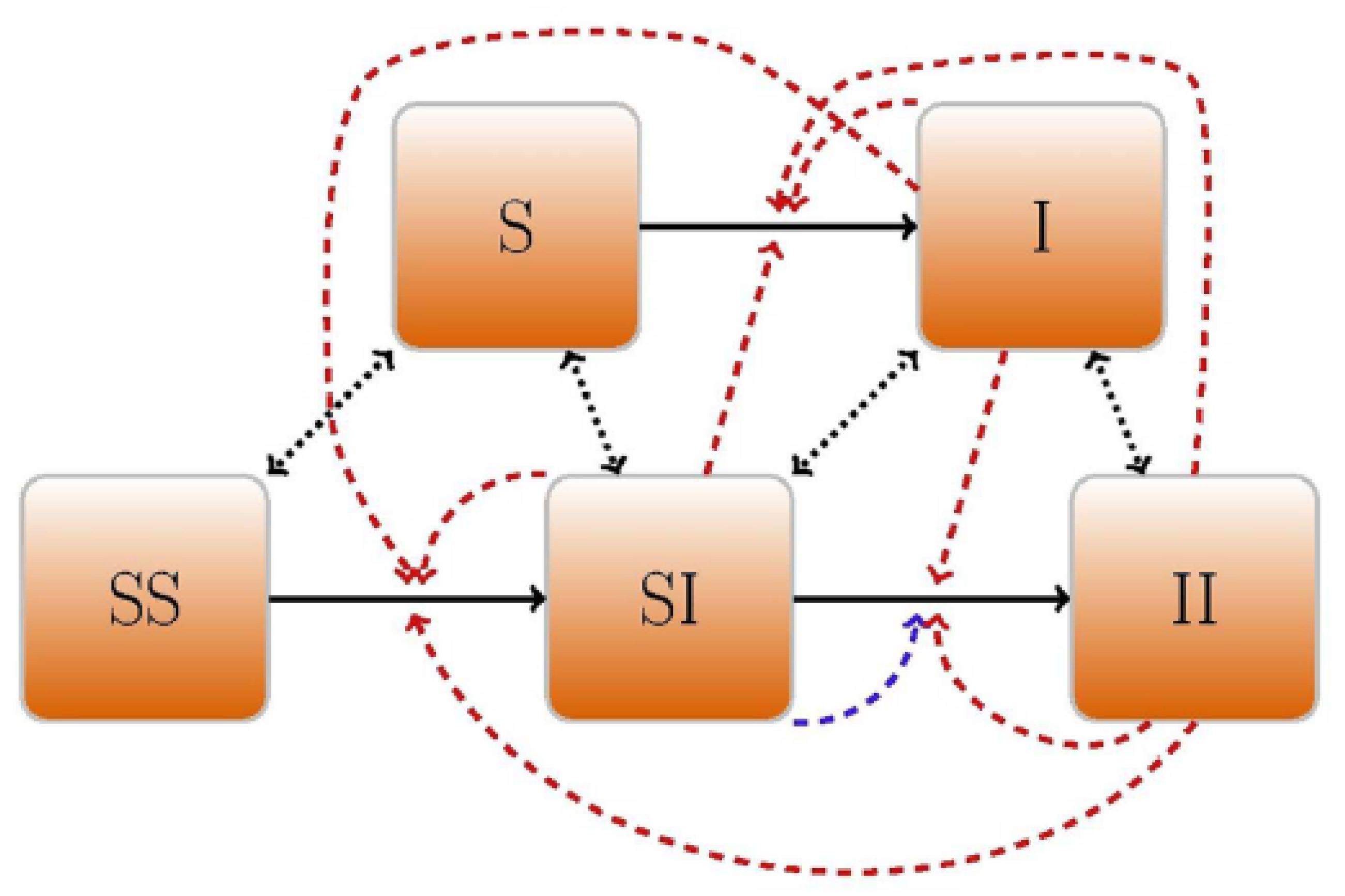
3.6. Contact Structure and Partnership Dynamics

Numerous utilized models of HIV eco-evolutionary dynamics utilize implied models that include the normal impacts of sexual contact given a concrete couple without impersonating the unequivocal dynamics of the configuration of a partner relationship [38]. Since our motivation stems from the fact that we are interested in exploring the way that issues around virulence evolution rely on the modeled contact structure, we examine a model with growing complexity levels in the contact structure, but at the same time, rearrange several of the remaining epidemiological forms (like the history of HIV as a within-host).

Figure 3 presents a schematic representation of the proposed model with explicit contact structure considering explicitly partnership dynamics [39]. Non-instantaneous partnership formation, which concerns people that are without any partner and spend a period as uncoupled, is presumed in the above schematic representation and comprises five categories related to different types of disease as well as values of partnership. Concretely, the five states are the following:

• Single (uncoupled) susceptible (or sensitive) individuals (S);
• Single infected (or contaminated) individuals (I);
• Concordant negative couples (i.e., susceptible–susceptible, $SS$) when both partners are susceptible;
• Discordant couples (i.e., susceptible–infected, $SI$);
• Concordant positive couples (i.e., infected–infected, $II$) when both partners are infectious.

Regarding schematic representation, solid arrows represent infection transitions (e.g., S towards I), dotted arrows exhibit partnership dialysis and configuration (e.g., S towards $SI$) and dashed arrows represent impacts on the rate of the infection, indicating transmission among the nodes of the pair (with blue color) as well as transmission among the nodes of an uncoupled pair (with red color).

The values of single (i.e., uncoupled) susceptible and infected people generate the rate of the configuration of each pair. Furthermore, associations and relationships among two individuals can either be suspended or even be modified into other types of relationships by infecting one out of two individuals. This corresponding model also incorporates another type of contact, namely when both individuals are uncoupled as well as individuals related to other partnerships. This means that these susceptible partners and susceptible uncoupled individuals in any sort of association can also be contaminated by infected partners or infected uncoupled individuals in any sort of association.

4. HIV Transmission Simulation of Biological Network

The propagation of the AIDS syndrome, triggered by the HIV virus, in a sample of infusing drug users, is introduced and thoroughly discussed in this section. Several virus propagation scenarios with various diverse parametric transmission modes as well as syndrome investigations during this propagation are comprehensively utilized.

4.1. Proposed Model

In the European Union, it has been shown that 18 million of its population are drug users, which is $5\%$ of the entire population (Retrieved 27 April 2021, from https://www.emcdda.europa.eu/). It is worth noting that out of $5\%$, a percentage equal to $0.63\%$ is attributed to individuals that are HIV infected via shared needles [40]. In light of the above information, the present work examines the propagation of the virus through all injected drug users, with the average transmission of the epidemic being multiple syringes used by various users.

The proposed model addresses the following issues by utilizing Boolean variables:

• Is the individual aware of carrying the infection or not?
• Has the syringe been given to more than one individual or not?
• Is the individual aware of being infected or not?

This proposed model simulates the spread of HIV through sexual transmission within a small isolated human population. HIV can be transmitted in several ways, where sexual contact can be considered as the most common and widespread. However, HIV can also be transmitted with the use of syringes shared through blood transfusions of injecting drug users. Another transmission type could be through women with HIV that can transmit the virus to their babies before or during birth, or even later through breastfeeding.

The proposed method also determines, by means of a variable, the portion of the population that will be manually infected. As a result, when simulating the alternations of input data, new questions and potential problems arise as well as more distinctive outcomes occur. In this study, we based our proposed model by taking into consideration the following aspects:

• For how long will the individual use the syringe?
• How many individuals will use clean (new) needles?
• How many individuals share simultaneously the same needle?
• How often are individuals tested by a physician?

There are auxiliary input variables in the system, which provide the possibility to manually change the data of the model in order to come up with different outcomes and outputs. As a result, the model displays during the simulation the number of infected individuals and is aware of the disease percentage as well as the rate of infection on a weekly basis.

4.2. Random Graph

The equal probability of each pair of individuals concerning the aspect of contact, regardless of the other pairs, is based on the theory of the Erdös–Renyi random graph, as depicted in Algorithm 1. However, an epidemic needs even more time for the spreading to be achieved, so we alternated the transmission of the syndrome into the epidemic transiently contact model accordingly our proposed model, which is more appropriate.

Algorithm 1 Epidemic Transiently Contact Model.

1: input All possible edges are considered and included in the graph with equal probability p 2: input Variable d that specifies the possibility of the unidirectional edges to be equally modified, i.e., if they are reciprocal 3: for each node i do 4:   for each node $j=i+1\cdots N$ do 5:     Set a random number u between 0 and 1 uniformly 6:     if  $p>u$  then 7:      Create a mutual (reciprocal) edge between node i and node j 8:     else 9:      if  $d>u$  then 10:       Create a directed edge from node i to node j 11:       Create a directed edge from node j to node i 12:      else 13:       Create a directed edge from node i to node j 14:       Set a randomly chosen node h from the set of all nodes except for i and j uniformly 15:       Create a directed edge from node h to node i 16:      end if 17:     end if 18:   end for 19: end for

The overall time complexity of the algorithm to generate a random graph of N nodes under the epidemic transiently contact model is $\mathsf{\Theta }\left(N^2\right)$ as this is the time complexity to execute the two "for" loops. Specifically, for each new step, the algorithm acts in $\mathsf{\Theta }\left(N\right)$ if one max directed edge per new node is created; otherwise, the complexity is $\mathsf{\Theta }\left(NM\right)$ if M the max directed edges per new node is created.

As aforementioned, we have modified the Erdös–Renyi random graph in the way that there is some dependence on whether or not the edges are present. This approach is taken into consideration because in many practical problems, the vertices are in fact randomly positioned in some geometric space (usually Euclidean). Furthermore, two vertices are adjacent if and only if the distance between them (in some specified norm) is less than a certain quantity. These corresponding points are usually uniformly distributed in ${[0,1]}^n$.

In the present manuscript, we tried to incorporate some basic notations from the random-duster model by biasing the formula for the probability of a set of edges in order to favor certain kinds of graphs arising. In this kind of model, given a graph $G=G(V,E)$ and a set of edges $A\subseteq E$, let $c(V,A)$ denote the number of components of the graph in which the vertices are denoted by V and the corresponding set of edges is denoted by A. Then, the probability that the edges that arise are exactly those in A is [41]:

$$\frac{p^{\left|A\right|}{(1-p)}^{\left|E\right|-\left|A\right|}{q}^{c(V,A)}}{{\sum }_{F\subseteq E}^{}{p}^{\left|F\right|}{(1-p)}^{\left|E\right|-\left|F\right|}{q}^{c(V,F)}}$$

(10)

where q is a positive integer used for favoring specific elements of a concrete graph. Namely, observe that when q is equal to 1, the Erdös–Renyi model is recovered. In addition, if $q>1$, graphs with many components are favored, whereas if $q<1$, the connected graphs are favored. Notice that the study of this model is closely linked to percolation theory and statistical physics.

4.3. Implementation

In the current paper, the problem of the transmission of HIV through injectable drugs in Europe is presented. Thus, according to the data presented by the European Drug Report, a small sample was adapted to the simulation due to the decrease in percentage of users in Europe in recent years. More specifically, the percentage of injecting drug users diagnosed with AIDS has dropped by almost $40\%$ as compared to the previous decade (Retrieved 27 April 2021, from https://www.emcdda.europa.eu/system/files/publications/11364/20191724_TDAT19001ENN_PDF.pdf). The sample used in the implementation is 300 as well as 500 users.

In addition to these samples, according to the study aforementioned [17], we consider a $0.63\%$ disease possibility for the AIDS virus; based on the above, the percentage of the population that is initially infected and enters the model, corresponds to $0.63\%$ of the entity. An important part of the application is considered the sharing of the same needle among drug individuals of the sample, which is implemented by the system’s random selection; if a person uses a syringe that “carries” the virus, there is $100\%$ probability of becoming infected. Another issue that has to be taken into account is that after about two years (i.e., 100 weeks), the symptoms of the syndrome begin to appear.

For the verification of our proposed methodology, four different scenarios have been implemented, as shown in

Table 2. Four different scenarios.

Scenario	1	2	3	4
Number of Users	300	300	500	500
Number of Tests per Year	1	2	1	2

. More specifically, Table 2 and

Table 3. Data of the twelve examples for four different scenarios.

Features	1	2	3	4	5	6	7	8	9	10	11	12
Percentage of Fuzziness	0% Fuzzy			10% Fuzzy			30% Fuzzy			50% Fuzzy
Shared Syringe	10	0	7	9	0	7	7	0	6	5	0	4
New Syringe	0	10	3	0	9	2	0	7	1	0	5	1
Fuzzy	0	0	0	1	1	1	3	3	3	5	5	5

present the percentages of fuzziness, which has been studied during the experiments. In the first part (out of four) of Table 3, no fuzziness was applied, while in the other three examples, percentages of fuzziness equal to $10\%$, $30\%$, and $50\%$, respectively, were applied. The primary research reason for choosing the specific scenarios is twofold. First, the comparison between the absence of fuzziness and different percentages of fuzziness will provide us with important insights. Second, the three different percentages are thoroughly selected until the percentage of $50\%$ because, if the results exceed this upper bound, the results will not be meaningful in terms of the problem we are trying to resolve.

From the two above-mentioned tables, the results shown in

Table 4. People regarding the first scenario for a different number of weeks.

Option of Illness	100	390	1390	2390	3930
0% Fuzzy—1st example
AIDS-	298	290	240	142	126
AIDS+	0	2	41	138	174
AIDS?	2	8	19	20	0
0% Fuzzy—2nd example
AIDS-	298	298	298	298	298
AIDS+	0	2	2	2	2
AIDS?	2	0	0	0	0
0% Fuzzy—3rd example
AIDS-	297	288	200	135	119
AIDS+	0	5	63	156	181
AIDS?	3	7	37	9	0
10% Fuzzy—4th example
AIDS-	293	288	191	135	130
AIDS+	3	5	74	162	170
AIDS?	4	7	35	3	0
10% Fuzzy—5th example
AIDS-	298	298	298	298	298
AIDS+	0	2	2	2	2
AIDS?	2	0	0	0	0
10% Fuzzy—6th example
AIDS-	296	285	217	148	128
AIDS+	0	9	55	141	172
AIDS?	4	6	28	11	0
30% Fuzzy—7th example
AIDS-	297	288	234	178	145
AIDS+	0	4	54	109	155
AIDS?	3	8	12	13	0
30% Fuzzy—8th example
AIDS-	298	298	298	298	298
AIDS+	0	2	2	2	2
AIDS?	2	0	0	0	0
30% Fuzzy—9th example
AIDS-	292	290	258	189	138
AIDS+	2	4	32	88	162
AIDS?	4	6	10	23	0
50% Fuzzy—10th example
AIDS-	294	285	213	153	136
AIDS+	2	5	64	134	164
AIDS?	4	10	23	13	0
50% Fuzz—11th example
AIDS-	298	298	298	298	298
AIDS+	0	2	2	2	2
AIDS?	2	0	0	0	0
50% Fuzzy—12th example
AIDS-	296	294	277	264	210
AIDS+	0	2	16	31	90
AIDS?	4	4	7	5	0

,

Table 5. People regarding the second scenario for a different number of weeks.

Option of Illness	100	390	1390	2390	3930
0% Fuzzy—1st example
AIDS-	295	294	290	284	284
AIDS+	2	4	4	16	16
AIDS?	3	4	6	0	0
0% Fuzzy—2nd example
AIDS-	298	298	298	298	298
AIDS+	0	2	2	2	2
AIDS?	2	0	0	0	0
0% Fuzzy—3rd example
AIDS-	295	292	291	291	291
AIDS+	0	5	9	9	9
AIDS?	5	3	0	0	0
10% Fuzzy—4th example
AIDS-	295	290	258	254	254
AIDS+	1	4	39	46	46
AIDS?	4	6	3	0	0
10% Fuzzy—5th example
AIDS-	298	298	298	298	298
AIDS+	0	2	2	2	2
AIDS?	2	0	0	0	0
10% Fuzzy—6th example
AIDS-	296	292	273	273	273
AIDS+	1	3	27	27	27
AIDS?	3	5	0	0	0
30% Fuzzy—7th example
AIDS-	296	288	261	244	244
AIDS+	0	5	35	56	56
AIDS?	4	7	4	0	0
30% Fuzzy—8th example
AIDS-	298	298	298	298	298
AIDS+	0	2	2	2	2
AIDS?	2	0	0	0	0
30% Fuzzy—9th example
AIDS-	294	288	278	278	278
AIDS+	2	5	22	22	22
AIDS?	4	7	0	0	0
50% Fuzzy—10th example
AIDS-	295	288	259	253	253
AIDS+	0	5	36	47	47
AIDS?	5	7	5	0	0
50% Fuzzy—11th example
AIDS-	298	298	298	298	298
AIDS+	0	2	2	2	2
AIDS?	2	0	0	0	0
50% Fuzzy—12th example
AIDS-	296	294	293	293	293
AIDS+	0	4	7	7	7
AIDS?	4	2	0	0	0

,

Table 6. People regarding the third scenario for a different number of weeks.

Option of Illness	100	390	1390	2390	3930
0% Fuzzy—1st example
AIDS-	491	489	385	260	211
AIDS+	2	3	78	214	289
AIDS?	7	8	37	26	0
0% Fuzzy—2nd example
AIDS-	497	497	497	497	497
AIDS+	0	3	3	3	3
AIDS?	3	0	0	0	0
0% Fuzzy—3rd example
AIDS-	491	483	312	190	172
AIDS+	1	4	131	294	328
AIDS?	8	13	57	16	0
10% Fuzzy—4th example
AIDS-	492	482	384	235	219
AIDS+	2	5	78	247	281
AIDS?	6	13	38	18	0
10% Fuzzy—5th example
AIDS-	497	497	497	497	497
AIDS+	0	3	3	3	3
AIDS?	3	0	0	0	0
10% Fuzzy—6th example
AIDS-	491	477	292	183	171
AIDS+	1	5	141	311	329
AIDS?	8	18	67	6	0
30% Fuzzy—7th example
AIDS-	491	479	283	169	173
AIDS+	1	4	140	322	329
AIDS?	8	17	77	9	0
30% Fuzzy—8th example
AIDS-	497	497	497	497	497
AIDS+	0	3	3	3	3
AIDS?	3	0	0	0	0
30% Fuzzy—9th example
AIDS-	492	475	294	231	223
AIDS+	1	8	151	261	275
AIDS?	7	17	55	8	0
50% Fuzzy—10th example
AIDS-	491	483	312	190	172
AIDS+	1	4	131	294	328
AIDS?	8	13	57	16	0
50% Fuzzy—11th example
AIDS-	497	497	497	497	497
AIDS+	0	3	3	3	3
AIDS?	3	0	0	0	0
50% Fuzzy—12th example
AIDS-	494	487	326	241	221
AIDS+	0	3	114	246	279
AIDS?	6	10	60	13	0

and

Table 7. People regarding the fourth scenario for a different number of weeks.

Option of Illness	100	390	1390	2390	3930
0% Fuzzy—1st example
AIDS-	487	477	417	391	376
AIDS+	3	13	74	106	123
AIDS?	10	10	9	2	0
0% Fuzzy—2nd example
AIDS-	497	497	497	497	497
AIDS+	0	3	3	3	3
AIDS?	3	0	0	0	0
0% Fuzzy—3rd example
AIDS-	486	481	413	343	318
AIDS+	4	14	70	141	182
AIDS?	10	5	17	16	0
10% Fuzzy—4th example
AIDS-	488	487	446	412	395
AIDS+	4	9	45	80	105
AIDS?	8	4	9	8	0
10% Fuzzy—5th example
AIDS-	497	497	497	497	497
AIDS+	0	3	3	3	3
AIDS?	3	0	0	0	0
10% Fuzzy—6th example
AIDS-	493	485	435	365	331
AIDS+	0	10	57	115	169
AIDS?	7	5	8	17	0
30% Fuzzy—7th example
AIDS-	488	485	448	422	400
AIDS+	5	10	43	73	100
AIDS?	7	5	9	5	0
30% Fuzzy—8th example
AIDS-	497	497	497	497	497
AIDS+	0	3	3	3	3
AIDS?	3	0	0	0	0
30% Fuzzy—9th example
AIDS-	489	486	420	352	340
AIDS+	3	9	62	140	160
AIDS?	8	5	18	8	0
50% Fuzzy—10th example
AIDS-	492	478	417	392	380
AIDS+	2	14	74	105	120
AIDS?	6	8	9	3	0
$50\%$ Fuzzy—11th example
AIDS-	497	497	497	497	497
AIDS+	0	3	3	3	3
AIDS?	3	0	0	0	0
50% Fuzzy—12th example
AIDS-	492	486	461	454	443
AIDS+	0	9	36	45	57
AIDS?	8	5	3	1	0

are depicted. Concretely, Table 4 and Table 5 introduce the outcomes of the first two scenarios where the sample is 300 individuals and they are obliged to carry out one and two tests per year, respectively. On the other hand, Table 6 and Table 7 present the results of the last two scenarios where the sample is 500 individuals and are obliged to carry out one and two tests per year, respectively.

5. Results

In the following, Table 4, Table 5, Table 6 and Table 7 present the results for the four above-mentioned scenarios. Please notice the following three categories of users.

• AIDS-: users not infected by HIV.
• AIDS+: users infected by HIV and they know it (they have been tested).
• AIDS?: users who have no knowledge if they are (or not) infected by HIV and they have not passed the one year time limit in order to be tested.

First Scenario: Table 4 shows that examples 2, 5, 8, and 11 achieve the same results. This is due to the fact that all users use a new syringe for every drug use, thus resulting in the same percentage of infection in the sample, for example, $0.67\%$. Moreover, in examples 1, 4, 7, and 10, users sharing illegal substances are many and no one uses a new syringe. As a result, we can observe that the disease spreading increases rapidly in all four examples, although there is a large percentage of fuzziness in examples 4 (with $10\%$), 7 (with $30\%$) and 10 (with $50\%$). In these examples, the rates of infection range from $40\%$ to $56\%$ as we do not know what the whole sample is doing; that is, when we have a percentage of fuzziness equal to $30\%$, we actually do not know what 3 out of 10 users are doing (sharing or using a new syringe in each contact).

Regarding examples 3, 6, 9, and 12, the simulation in the sample is closer to reality; that is, some of the users are using illicit substances with a new syringe. An increase in the spread of the virus is depicted, as disease spreading rates range from $25\%$ to $55\%$. In addition, the largest value is presented in example 6 with the percentage of fuzziness equal to $10\%$, whereas the lowest value is presented in example 12 with a percentage of fuzziness equal to $50\%$. These results are justified as the percentage of fuzziness in example 6 is less than the corresponding value in example 12.

It should be noted that, in these examples, each user has been forced to do an HIV test once a year.

Second Scenario: Table 5 shows, similarly to Table 4, that examples 2, 5, 8, and 11 achieve the same results. As a result, the percentage of infection in the sample remained the same, for example, $0.67\%$. Moreover, in examples 1, 4, 7, and 10, users sharing illegal substances are 10, 9, 7 and 5 out of 10 (according to Table 3 and the corresponding fuzziness) and no one uses a new syringe. Thus, it is observed that the disease spreading increases in an even more rapid way, in all four examples, than in Table 4.

Furthermore, this increase reaches its biggest value in a shorter time, for example, 2390 weeks in all four examples, despite the fact that fuzziness plays an important role in the last three examples. In these examples, the rates of infection range from $5\%$ to $20\%$ and this decrease, compared to Table 4, is due to the number of mandatory HIV test samples submitted over time, which are two instead of one.

As in Table 4, results in examples 3, 6, 9, and 12 present a sharp decrease in virus spreading. The disease spreading values range from $1.3\%$ to $9\%$, with the largest value being in example 6 with the percentage of fuzziness equal to $10\%$. On the other hand, the lowest values are presented in examples 1 and 12 with the percentage of fuzziness equal to $0\%$ and $50\%$, respectively.

Third Scenario: The examples 2, 5, 8, and 11 in Table 6 perform exactly like the corresponding ones in previous Table 4 and Table 5. The only difference lies in the rate of infection, which has a value equal to $0.8\%$ (the infection rate has a starting value equal to $0.8\%$ and not $0.63\%$ as the probability of infection lies between $3.15$ and 500 under the $500\times 0.0063=3.15$). This is justified as all users use a new syringe in every drug use.

Examples 1, 4, 7, and 10 perform similarly to Table 5, whereas the rates of infection range from $50\%$ to $62\%$. We also anticipated that examples 3, 6, 9, and 12 would be closer to reality, and the values prove our assumptions. In addition, a marked increase in the spread of the virus is observed where the rates of infection range from $52\%$ to $68\%$. More specifically, the highest value is achieved in example 9 with the percentage of fuzziness equal to $30\%$, while the lowest value is achieved in example 12 with the percentage of fuzziness equal to $50\%$.

Fourth Scenario: As we anticipated, the results in examples 2, 5, 8, and 11 in Table 7 perform in the same way as in previous Tables. Moreover, the rate of infection has a value equal to $0.8\%$, as in Table 6. In examples 1, 4, 7, and 10, no new syringe is used and the number of users sharing illegal substances is 10, 9, 7 and 5 out of 10, respectively. It is also observed that the increase in the disease spread does not rise in a quick way and thus, it achieves more promising results for all the corresponding examples. The values of infection in the sample range from $13\%$ to $25\%$, and this is presented due to the two mandatory HIV test samples submitted over time.

Finally, we noticed a pronounced decrease in the spread of the virus in terms of the corresponding results of Table 5, regarding examples 3, 6, 9, and 12. More specifically, the rates of infection range from $9.5\%$ to $36\%$, where the highest value is achieved when the percentage of fuzziness is equal to $0\%$, and the lowest value is achieved when the percentage of fuzziness is equal to $50\%$.

5.1. Comparing All Four Scenarios

Table 8. Comparison between the four scenarios for a different number of weeks by considering the 3rd example with $0\%$ fuzzy.

Option of Illness	100	390	1390	2390	3930	100	390	1390	2390	3930
	1st scenario—1 test—300 users					3rd scenario—1 test—500 users
AIDS-	297	288	200	135	119	491	483	312	190	172
AIDS+	0	5	63	156	181	1	4	131	294	328
AIDS?	3	7	37	9	0	8	13	57	16	0
	2nd scenario—2 tests—300 users					4th scenario—2 tests—500 users
AIDS-	295	292	291	291	291	486	481	413	343	318
AIDS+	0	5	9	9	9	4	14	70	141	182
AIDS?	5	3	0	0	0	10	5	17	16	0

,

Table 9. Comparison between the four scenarios for a different number of weeks by considering the 6th example with $10\%$ fuzzy.

Option of Illness	100	390	1390	2390	3930	100	390	1390	2390	3930
	1st scenario—1 test—300 users					3rd scenario—1 test—500 users
AIDS-	296	285	217	148	128	491	477	292	183	171
AIDS+	0	9	55	141	172	1	5	141	311	329
AIDS?	4	6	28	11	0	8	18	67	6	0
	2nd scenario—2 tests—300 users					4th scenario—2 tests—500 users
AIDS-	296	292	273	273	273	493	485	435	365	331
AIDS+	1	3	27	27	27	0	10	57	115	169
AIDS?	3	5	0	0	0	7	5	8	17	0

,

Table 10. Comparison between the four scenarios for a different number of weeks by considering the 9th example with $30\%$ fuzzy.

Option of Illness	100	390	1390	2390	3930	100	390	1390	2390	3930
	1st scenario—1 test—300 users					3rd scenario—1 test—500 users
AIDS-	292	290	258	189	138	492	475	294	231	223
AIDS+	2	4	32	88	162	1	8	151	261	275
AIDS?	4	6	10	23	0	7	17	55	8	0
	2nd scenario—2 tests—300 users					4th scenario—2 tests—500 users
AIDS-	294	288	278	278	278	489	486	420	352	340
AIDS+	2	5	22	22	22	3	9	62	140	160
AIDS?	4	7	0	0	0	8	5	18	8	0

and

Table 11. Comparison between the four scenarios for a different number of weeks by considering the 12th example with $50\%$ fuzzy.

Option of Illness	100	390	1390	2390	3930	100	390	1390	2390	3930
	1st scenario—1 test—300 users					3rd scenario—1 test—500 users
AIDS-	296	294	277	264	210	494	487	326	241	221
AIDS+	0	2	16	31	90	0	3	114	246	279
AIDS?	4	4	7	5	0	6	10	60	13	0
	2nd scenario—2 tests—300 users					4th scenario—2 tests—500 users
AIDS-	296	294	293	293	293	492	486	461	454	443
AIDS+	0	4	7	7	7	0	9	36	45	57
AIDS?	4	2	0	0	0	8	5	3	1	0

depict the results from the virus spreading scenarios with the most plausible values (i.e., some users use illegal substances with a new syringe while others share the same); that is, we have used the results from examples 3, 6, 9 and 12. The results are grouped by the value of fuzziness, and both population samples (i.e., 300 and 500 individuals) are displayed in order for the comparison to be manifested.

In more detail, in Table 8, with a fuzziness of $0\%$, the increase in the spread of the virus as the number of weeks increases is clearly visible since this spread in the results concerning the one mandatory blood test per year (scenarios 1 and 3), for both samples, is fairly fast with spread rates ranging from $34\%$ to $52\%$. On the other hand, assuming two mandatory blood tests per year (scenarios 2 and 4), the rates of the virus spread range from about $1.3\%$ to $36\%$, respectively.

The results in Table 9 with fuzziness of $10\%$ are almost the same as in Table 8. Specifically, for scenarios 1 and 3, the increase in the virus spreading is fast where the spread percentages present values from about $25\%$ to $55\%$, respectively. On the other hand, in scenarios 2 and 4, we notice that the virus spreading does not increase so rapidly as it presents values from about $9\%$ to $17\%$, respectively.

Table 10 presents the results where the percentage of fuzziness is equal to $30\%$. We can observe that the values are identical with the ones of the previous tables. Concretely, for scenarios 1 and 3, the increase in the spread of the virus in both samples ranges from about 45–$68\%$, respectively. While in scenarios 2 and 4, we notice that these percentages are adequately lower, presenting values from about $1.3$–$8\%$, respectively.

Finally, Table 11 depicts the results with a percentage of fuzziness equal to $50\%$. As mentioned above, the increase for all four scenarios are almost identical, as in the three previous tables. The increase in virus spreading, for scenarios 1 and 3, ranges from about 25–$52\%$, respectively, whereas when considering scenarios 2 and 4, the increase takes values from about $1.3$–$9.5\%$.

5.2. Discussion

Studying complex networks can solve various real-world problems and can be applied to a variety of scientific fields. They make it possible to investigate any scientific network according to the requirements of each real-world area and, of course, based on the input data of each concrete network. Complex networks also provide a view of the composition entities of a network resulting in the creation of arbitrarily configured networks. Additionally, it is possible for these entities to be at any moment removed from the network. Because of their efficiency described above, complex networks are becoming both popular and attractive.

It is of major importance to notice that studying and understanding the processes utilized in complex networks presents new horizons for researchers to investigate and solve many problems (e.g., diseases diffusion and propagation, mutations) in terms of these networks. The science of molecular biology considers distinct complex networks consisting of numerous interacting parts with different structures, such as enzymes, genes, and proteins. In addition, in the area of epidemiology, beyond the examination of complex networks, the corresponding complex networks are initially analyzed, then modeled and finally simulated in the form of toolboxes.

Any similar approaches in the context of epidemics fail in understanding the principles of random graphs and especially in the corresponding problem we are investigating. Regarding fuzzy estimators, let us assume that we are interested in answering the question “What is the fuzzy probability that a very sexually active individual will develop AIDS?”. Then, the fuzzy ratio is considered as we are dealing with the conditional probability that this specific individual will develop AIDS with a certain speed given that he/she is subject to a certain risk due to his/her sexual activity level.

According to the individuals who make up each society (300 and 500 people), a significant difference regarding the results was observed. More specifically, when a run of our proposed technique was performed in a larger sample of people and after many tests, it was found that the sample with the 500 individuals proportionally achieved the greatest improvement in the results in terms of virus transmission with respect to the same conditions and parameters. This results in greater precision of the model in samples approaching the real world.

6. Conclusions and Future Work

In this paper, a fuzzy implementation based on complex network theory was introduced. In particular, the propagation of a corresponding disease (e.g., AIDS) to a sample of individuals with specific characteristics was simulated by implementing two different models of complex networks. The first scheme utilized the Erdös—Renyi model considering that the sample was selected from the original population and assuming that the relationships between individuals follow the random graph; also, in this model, the virus transmission is based on the epidemic contact transient model. On the other hand, in the second scheme utilized, different scenarios were investigated and performed and also different conditions within the sample were measured in order to obtain the results through the process of fuzzy simulations, which cannot be effectively implemented in the real world. These results depict the evolution of formalism among the individuals of the concrete population. Furthermore, we can argue that this tool, according to the information obtained, can also be a preventive application to various diseases.

The study of multi-virus networks as well as the investigation of different epidemic models are some of the future expansions of our work. In addition, another future work that can extend our proposed application is the integration of distinctive algorithmic analytic methods along with the introduction of the theory of dynamic systems. Further analytical experimental evaluation of the application can be considered as a critical point since the system provides new examples through its auxiliary input variables. Finally, after simulating the model, we explored the notion that incorporating effective heuristics in terms of temporal graphs is something to be outlined and attracts a lot of interest.

References

1. West, D.B. Introduction to Graph Theory; Prentice Hall: Upper Saddle River, NJ, USA, 2001; Volume 2. [Google Scholar]
2. Newman, M.E.J. The Structure and Function of Complex Networks. SIAM Rev. 2003, 45, 167–256. [Google Scholar] [CrossRef] [Green Version]
3. Boccaletti, S.; Latora, V.; Moreno, Y.; Chavez, M.; Hwang, D.U. Complex Networks: Structure and Dynamics. Phys. Rep. 2006, 424, 175–308. [Google Scholar] [CrossRef]
4. Power, J.D.; Cohen, A.L.; Nelson, S.M.; Wig, G.S.; Barnes, K.A.; Church, J.A.; Vogel, A.C.; Laumann, T.O.; Miezin, F.M.; Schlaggar, B.L.; et al. Functional Network Organization of the Human Brain. Neuron 2011, 72, 665–678. [Google Scholar] [CrossRef] [Green Version]
5. Shang, Y. Mixed SI (R) Epidemic Dynamics in Random Graphs with General Degree Distributions. Appl. Math. Comput. 2013, 219, 5042–5048. [Google Scholar] [CrossRef]
6. Nowzari, C.; Preciado, V.; Pappas, G. Analysis and Control of Epidemics: A Survey of Spreading Processes on Complex Networks. IEEE Control. Syst. 2016, 36, 26–46. [Google Scholar]
7. Pastor-Satorras, R.; Castellano, C.; Mieghem, P.V.; Vespignani, A. Epidemic Processes in Complex Networks. Rev. Mod. Phys. 2015, 87, 925–979. [Google Scholar] [CrossRef] [Green Version]
8. Li, C.H.; Tsai, C.C.; Yang, S.Y. Analysis of Epidemic Spreading of an SIRS Model in Complex Heterogeneous Networks. Commun. Nonlinear Sci. Numer. Simul. 2014, 19, 1042–1054. [Google Scholar] [CrossRef]
9. Fofana, A.M.; Hurford, A. Mechanistic Movement Models to Understand Epidemic Spread. Philos. Trans. R. Soc. Lond. Biol. Sci. 2017, 372, 20160086. [Google Scholar] [CrossRef]
10. Wang, W.; Tang, M.; Stanley, E.; Braunstein, L.A. Unification of Theoretical Approaches for Epidemic Spreading on Complex Networks. Rep. Prog. Phys. 2017, 80, 036603. [Google Scholar] [CrossRef]
11. Prettejohn, B.J.; Berryman, M.J.; McDonnell, M.D. Methods for Generating Complex Networks with Selected Structural Properties for Simulations: A Review and Tutorial for Neuroscientists. Front. Comput. Neurosci. 2011, 2011. [Google Scholar] [CrossRef] [Green Version]
12. Faria, N.R.; Rambaut, A.; Suchard, M.A.; Baele, G.; Bedford, T.; Ward, M.J.; Tatem, A.J.; Sousa, J.D.; Arinaminpathy, N.; Pépin, J.; et al. The Early Spread and Epidemic Ignition of HIV-1 in Human Populations. Science 2014, 346, 56–61. [Google Scholar] [CrossRef] [Green Version]
13. Massad, E.; Ortega, N.R.S.; Struchiner, C.J.; Burattini, M.N. Fuzzy Epidemics. Artif. Intell. Med. 2003, 29, 241–259. [Google Scholar] [CrossRef]
14. Zadeh, L.A. Fuzzy Sets. Inf. Control. 1965, 8, 338–353. [Google Scholar] [CrossRef] [Green Version]
15. Zimmermann, H.J. Fuzzy Set Theory and Its Applications; Springer Science & Business Media: Berlin/Heidelberg, Germany, 2011. [Google Scholar]
16. Goguen, J.A. The Logic of Inexact Concepts. Synthese 1969, 19, 325–373. [Google Scholar] [CrossRef]
17. Lefevr, N.; Margariti, S.; Kanavos, A.; Tsakalidis, A. An Implementation of Disease Spreading over Biological Networks. In Proceedings of the 18th International Conference on Engineering Applications of Neural Networks (EANN), Athens, Greece, 25–27 August 2017; pp. 559–569. [Google Scholar]
18. Easley, D.A.; Kleinberg, J.M. Networks, Crowds, and Markets-Reasoning about a Highly Connected World; Cambridge University Press: Cambridge, UK, 2010. [Google Scholar]
19. Wasserman, S.; Faust, K. Social Network Analysis: Methods and Applications; Cambridge University Press: Cambridge, UK, 1994; Volume 8. [Google Scholar]
20. Dorogovtsev, S.N. Lectures on Complex Networks; Oxford University Press: New York, NY, USA, 2010; Volume 24. [Google Scholar]
21. Newman, M.E.J. Networks: An Introduction; Oxford University Press Inc.: New York, NY, USA, 2010. [Google Scholar]
22. Mao, G.; Zhang, N. Analysis of Average Shortest-Path Length of Scale-Free Network. J. Appl. Math. 2013, 2013, 865643:1–865643:5. [Google Scholar] [CrossRef]
23. Ahuja, R.K.; Magnanti, T.L.; Orlin, J.B. Network Flows: Theory, Algorithms and Applications; Prentice Hall: Upper Saddle River, NJ, USA, 1993. [Google Scholar]
24. Crucitti, P.; Latora, V.; Marchiori, M. Model for Cascading Failures in Complex Networks. Phys. Rev. E 2004, 69, 045104. [Google Scholar] [CrossRef] [PubMed] [Green Version]
25. Li, Y.; Shang, Y.; Yang, Y. Clustering Coefficients of Large Networks. Inf. Sci. 2017, 382–383, 350–358. [Google Scholar] [CrossRef]
26. Watts, D.J. Small Worlds: The Dynamics of Networks between Order and Randomness; Princeton University Press: Princeton, NY, USA, 1999. [Google Scholar]
27. Erdös, P.; Rényi, A. On Random Graphs I. Publ. Math. Debr. 1959, 6, 290–297. [Google Scholar]
28. Adamic, L.A.; Lukose, R.M.; Puniyani, A.R.; Huberman, B.A. Search in Power-Law Networks. Phys. Rev. E 2001, 64, 046135. [Google Scholar] [CrossRef] [PubMed] [Green Version]
29. Barabási, A.L.; Albert, R. Emergence of Scaling in Random Networks. Science 1999, 286, 509–512. [Google Scholar] [CrossRef] [Green Version]
30. Pastor-Satorras, R.; Vespignani, A. Evolution and Structure of the Internet: A Statistical Physics Approach; Cambridge University Press: Cambridge, UK, 2007. [Google Scholar]
31. Anastasio, T.J. Tutorial on Neural Systems Modeling; Sinauer Associates Incorporated Publishers: Sunderland, MA, USA, 2009. [Google Scholar]
32. Rothman, K.J.; Greenland, S.; Lash, T.L. Modern Epidemiology; Wolters Kluwer Health/Lippincott Williams & Wilkins: Philadelphia, PA, USA, 2008. [Google Scholar]
33. Zadeh, L.A. Fuzzy Sets as a Basis for a Theory of Possibility. Fuzzy Sets Syst. 1999, 100, 9–34. [Google Scholar] [CrossRef]
34. Lee, C. Fuzzy Logic in Control Systems: Fuzzy Logic Controller I. IEEE Trans. Syst. Man, Cybern. 1990, 20, 404–418. [Google Scholar] [CrossRef] [Green Version]
35. Lee, C. Fuzzy Logic in Control Systems: Fuzzy Logic Controller II. IEEE Trans. Syst. Man, Cybern. 1990, 20, 419–435. [Google Scholar] [CrossRef]
36. Lin, C.; Lee, C.S.G. Neural-Network-Based Fuzzy Logic Control and Decision System. IEEE Trans. Comput. 1991, 40, 1320–1336. [Google Scholar] [CrossRef]
37. McClelland, J.L.; Cleeremans, A. Consciousness and Connectionist Models. Oxf. Companion Conscious. 2009, 5, 180–181. [Google Scholar]
38. Park, S.W.; Bolker, B.M. Effects of Contact Structure on the Transient Evolution of HIV Virulence. PLoS Comput. Biol. 2017, 13, e1005453. [Google Scholar] [CrossRef] [PubMed] [Green Version]
39. Champredon, D.; Bellan, S.; Dushoff, J. HIV Sexual Transmission is Predominantly Driven by Single Individuals Rather than Discordant Couples: A Model-Based Approach. PLoS ONE 2013, 8, e082906. [Google Scholar] [CrossRef] [PubMed]
40. Patel, P.; Borkowf, C.B.; Brooks, J.T.; Lasry, A.; Lansky, A.; Mermin, J. Estimating Per-Act HIV Transmission Risk: A Systematic Review. Aids 2014, 28, 1509–1519. [Google Scholar] [CrossRef] [PubMed]
41. Cannings, C.; Penman, D. Chapter 2: Models of Random Graphs and their Applications. Handb. Stat. 2003, 21, 51–91. [Google Scholar]
Figure 1. The Barabási–Albert model.
Mathematics 09 00977 g001
Figure 2. A Tree Network of an Epidemic Spread.
Mathematics 09 00977 g002
Figure 3. Schematic representation of model with explicit contact structure.
Mathematics 09 00977 g003