
Evolving Deep Learning Convolutional Neural Networks for Early COVID-19 Detection in Chest X-ray Images


1
Department of Electronic Engineering, Imam Khomeini Marine Science University of Nowshahr, Nowshahr 16846-13114, Iran
2
Institute of Artificial Intelligence, De Montfort University, Leicester LE1 9BH, UK
3
Cyber Technology Institute, De Montfort University, Leicester LE1 9BH, UK
*
Author to whom correspondence should be addressed.
Mathematics 2021, 9(9), 1002; https://0-doi-org.brum.beds.ac.uk/10.3390/math9091002
Submission received: 30 March 2021
/
Revised: 19 April 2021
/
Accepted: 26 April 2021
/
Published: 28 April 2021
(This article belongs to the Special Issue Swarm and Evolutionary Computation—Bridging Theory and Practice)
Abstract
:This article proposes a framework that automatically designs classifiers for the early detection of COVID-19 from chest X-ray images. To do this, our approach repeatedly makes use of a heuristic for optimisation to efficiently find the best combination of the hyperparameters of a convolutional deep learning model. The framework starts with optimising a basic convolutional neural network which represents the starting point for the evolution process. Subsequently, at most two additional convolutional layers are added, at a time, to the previous convolutional structure as a result of a further optimisation phase. Each performed phase maximises the the accuracy of the system, thus requiring training and assessment of the new model, which gets gradually deeper, with relevant COVID-19 chest X-ray images. This iterative process ends when no improvement, in terms of accuracy, is recorded. Hence, the proposed method evolves the most performing network with the minimum number of convolutional layers. In this light, we simultaneously achieve high accuracy while minimising the presence of redundant layers to guarantee a fast but reliable model. Our results show that the proposed implementation of such a framework achieves accuracy up to , thus being particularly suitable for the early detection of COVID-19.
1. Introduction
Early detection of COVID-19 is becoming ever more important to prevent patients from developing pneumonia [1]. Due to the delays with the production and implementation of the vaccination campaign, prevention plays a major role and a controlled prognosis is only possible if the protocol therapy [2] is applied since the very early stages. The Polymerase Chain Reaction (PCR) test is the primary method for detecting COVID-19 as it is more reliable than any other option available to practitioners in the health & care system [3,4,5,6]. However, PCR is laborious, very time-consuming, and sometimes difficult to process due to shortages of kits and delays in their delivery in many countries worldwide. On the contrary, X-ray images are broadly available, and scans come with significantly lower costs.
In this light, technology-driven alternative solutions can play a key role in achieving a more sustainable, logistically simpler, and more timely early detection of this disease. In the past, the research community in artificial Intelligence (AI) has actively engaged with the health & care sector and produced relevant neural, fuzzy and evolutionary classifiers for early diagnosis and prognosis [7,8,9,10,11]. Given the recent exceptional results obtained with Deep Learning (DL) for image processing, see e.g., [12,13,14,15], the most logical choice for designing early detection systems based on X-ray images is to employ this AI paradigm. In terms of implementation, the most successful DL architecture seems to be those based on Convolutional Neural Networks (CNNs), which have already been adopted in recent studies on COVID-19 detection [4,16,17,18,19].
Optimal tuning of DL systems is still an unsolved and challenging problem [20,21]. Established approaches to fine-tune parameters of a deep network are based on the formulation of such task as an optimisation problem, then solved numerically with e.g., the classic Conjugate Gradient (CG) solution method [22], reinforcement learning [23], or gradient free approaches where the hessian matrix is empirically approximate as in the “Krylov subspace” descent methods [24,25]. Amongst these, gradient-free methods are most commonly used as they are easy to implement and fast - hence suitable for scenarios considering several training samples. However, they require numerous manual parameter tuning to work optimally and have a sequential nature making them very difficult to implement in Graphics Processing Units (GPU). CG-based method are in contrast more accurate but significantly slower, thus requiring multiple CPUs and large amounts of RAM to be applicable to DL models [26,27].
An alternative approach to train AI models that is currently well-received by the research community consists in solving the aforementioned optimisation problem with heuristic algorithms, often nature-inspired ones as those mentioned in Section 2.3, which have been successfully employed in training support vector machines [28], clustering algorithms [8,29,30], autoencoders [10,31], fuzzy and neural systems [32,33]. An interesting approach referred to as “neuroevolution” is based on encoding different network structures in the form of candidate solutions of a Genetic Algorithm (GA) heuristic [34], thus evolving the optimal architecture of the network while training it. It is worth mentioning that such method is currently also available for DL neural models [35]. Similarly, further “evolutionary” classifiers have been proposed e.g., using multi-objective optimisation methods, as in [9], and more recent nature-inspired heuristics adapted to deal with convolutions structures [36,37]. Other adaptive convolutional frameworks worth mentioning are e.g., the “progressive unsupervised learning” strategies in [38,39,40], where a mechanism is designed to select a pre-trained deep CNN from a pool, and the “automatic CNN architecture selection” system proposed in [41] to emphasise the parameters in image classification problems, which also uses a GA. The latter are based on solid considerations, but do have some flaws in terms of convergence speed as the employed genetic algorithms require an extremely high computational budget to converge over the very large scale search space resulting from encoding entire deep CNNs in the form of candidate solutions. To avoid this a GA was used in [42] to optimise the hyperparameters of a 3-layer CNN, with promising results. However, this approach presents a clear limitation as it cannot be applied to all cases in which a 3-layer structure is not adequate. Generally, the optimal number of layers is unknown. Hence, it should be preferably found during the training/optimisation process, as done in [43] where the number of layers is dynamically and gradually increased with a simple, and slow, mutation-only evolutionary approach.
To overcome the aforementioned limitations, we propose an efficient optimisation-driven classification framework for early COVID-19 detection. The latter, returns a fine-tuned convolutional model as a result of a number of subsequent optimisation phases during which a “growing” DL model is built. This iterative process makes use of the so-called “biogeography-based optimisation” algorithm, as discussed in Section 2.3, for evolving classifiers. This proposed approach displays advantages in terms time and memory complexity and produces a detection system that, once fed with X-ray chest images, makes a fast decision (i.e., diagnosis) of high accuracy (up to ). Note that the end result necessarily uses a CNN architecture, but its structure is not fixed. Depending on data availability, the system can be restarted to generate the most suitable classifier with optimised hyperparameters. The main contributions of the proposed approach are
- a system that efficiently discovers DL models with growing depths, with no constraints on number of layers, thus optimising performances;
- a fast optimisation phase, making this method suitable also in devices plagued by modest computational capabilities;
- an practical encoding strategy for the convolutional structures to be “evolved” that allow for a practical model quality evaluation.
Hence, this piece of research does not aim at replacing PCR completely but at making the existing X-ray process, which is used anyway, faster and more reliable. By doing this, the posed method also facilitates decision-making in those uncertain cases that are difficult to deal with by naked eye, and minimise human error due to the high volume of X-ray images that radiologists are required to vision in peak periods.
The remainder of this article is organised as as follows:
- Section 2 reports the material and methods used in this study in terms of employed dataset and optimisation algorithm;
- Section 3 describes all the components forming the proposed system;
- Section 4 shows our results;
- Section 5 comments on the our achievements;
- Section 6 draws the conclusions of this study.
2. Materials and Methods
2.1. COVID-X-ray Dataset
We make use of the COVID X-ray-5k dataset [44]. This currently contains 2084 training and 3100 test samples amongst chest X-ray and CT images.
Note, that in the original release on 3 May 2020, this database contained 250 X-ray images of COVID-19 patients, from which 203 images are anterior-posterior view. However, this is constantly updated. Unlike lateral ones, the selected images are preferable for CVID-19 detection-as advised in [45] by board-certified radiologists. Moreover, expert radiologists evaluated the collected images and labelled 184 out of the 203 images as having clear signs of COVID-19. 100 images were randomly selected to form the test set, and the remaining 84 to form the training set. It should be noted that we do not deal with the remaining cases here, were experts did not detect clear signs of COVID-19. They require further research.
To be usable in DL models, that set of COVID-19 samples was increased to 420 via data augmentation techniques such as flipping, application of small rotations and adding small amount of distortions [45]. Supplementary images from the ChexPert dataset [46] were then used as non-COVID-19 images. Note that this dataset includes 224,316 chest X-ray images from 65,240 patients. Most importantly, it is worth highlighting that the considered non-COVID-19 entries include a variety of scenarios reporting healthy cases as well as cases of other diseases such as pneumonia. This aspect is key to unbiased training and makes it possible to understand if the classifier is capable of distinguishing from COVID-19 cases and other pulmonary diseases. From this dataset 2000 and 3000 non-COVID images were used for the training set and test set, respectively.
A summary of the images in the final (i.e., employed) version the dataset is given in Table 1.
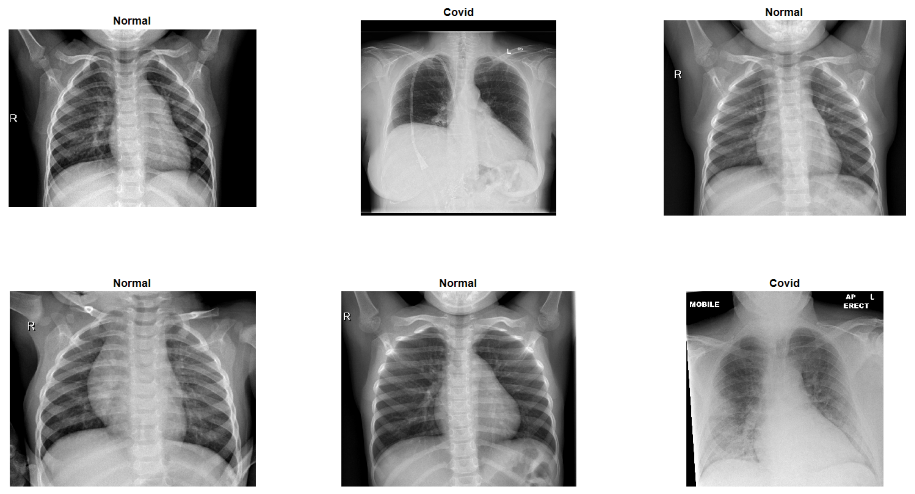
Figure 1 shows six random sample images from the COVID-X-ray-5k dataset, including two COVID-19 and four standard samples.
These images are used to train and validate our model, whose structure is the result of the iterative process explained in Section 3. The latter involves a number of optimisation processes where the hyperparameters of an “evolving” convolutional DL structure are fine-tuned with the optimiser introduced below in Section 2.3.
2.2. The Neural Network
As noted, CNNs have become the de-facto standard in image processing [47] and have been used successfully for X-ray analysis [4,11,16,17]. The network which is optimised by the algorithm lined out in the following section, is therefore a CNN. The type of layers possible in the network are convolutional, pooling, fully connected, and dropout layers. Table 2 shows the parameters which are emphasised during the process. These are the parameters which are typically selected manually when using a CNN. In our case, this is done using a specific optimisation approach. The resulting network will be called OptiDCNN in this paper.
According to the standard work on the use of meta-heuristics to tune hyperparameters of CNNs [42,43], the two most common problems encountered are:
- Underfitting if the CNN is too small.
- Overfitting if the CNN is too large.
Hence, the proposed approach has to start from a small CNN and sequentially grows it as needed to overcome these two drawbacks. Every time that the depth of the network is increased, the hyperparameters of the newly added blocks are optimised. This iterative process stops when adding more layers does not improve the classification performances. In this light, the returned classifier is optimised and cost-efficient, as requiring the minimum number of resources in terms of memory and computational cost while guaranteeing top performances.
All algorithms were implemented in Matlab. The deep learning toolbox was used for implementing the neural networks.
2.3. Biogeography-Based Optimisation
Biogeography-Based optimisation (BBO) [51] is a population-based heuristic for optimisation, sharing common aspects with several Evolutionary Algorithms (EAs) and Swarm Intelligence (SI) methods. Indeed, within the BBO framework candidate solutions in the search space have a probability of being selected for undergoing variation/perturbation operators, which is a typical feature of EAs [34], while not requiring “parents” to produce novel trial solutions, as in the SI paradigm [52]. In facts, each solution is perturbed individually and its new position is kept and compared only to the best candidate solution, , which gets updated any time a better position is found as in the so called “1-to-1 spawning” strategy. Like all nature-inspired heuristic approaches [53], BBO is general-purpose and based on a trial-and-error working logic which is iterated to produce near-optimal solutions of satisfactory quality - measured in terms of the so-called “fitness” value returned by the objective function. Note that the latter is commonly referred to as Habitat Suitability Index (HSI) in the BBO context. However, BBO has some characteristics making it particularly suitable for the optimisation problem at hand, such as (1) its flexibility in dealing with both discrete and real-valued optimisation problems, (2) its self-adaptive capabilities and facileness in tuning its parameters, and (3) its algorithmic overhead and converge speed. Indeed, in [51], BBO is compared to to other classic EAs and SI algorithms in terms of time complexity and convergence capabilities and shown to be among the fastest algorithms under study while being robust and less keen to prematurely converge or stagnate-drawbacks plaguing also state-of-the-art algorithms [54]. This aspect is key in this study as our objective functions require the training of DL convolutional architectures of increasing depths-see Section 3-thus making fast-converging and robust optimisers preferable to those adding undesired time overheads to the proposed system. Implementation details on the BBO framework are available in [51,55]. However, for the sake of clarity, it is worth mentioning that BBO draws its inspiration from the biogeography theory, see [56,57], and exploits it as a search logic in which the so-called “habitats” encode n-dimensional solutions x in the search space. Within the biogeography metaphor, each design variable forming the habitat solution (i.e., with ) is referred to as “habitant”. Similarly to Evolution Strategies [34], each habitat (with where N is the population size) is associated with some control parameters that evolve and adapt during the optimisation process. These are the emigration () and immigration ( probabilities, and the mutation rates (), which control the generation of new candidate solutions to explore the search space to eventually converge within a neighborhood of the optimal solution. This algorithmic behaviour is obtained by defining the control parameters as monotone functions such that, in a maximisation context, habitants in a habitat with small HSI have higher and are more likely to emigrate to most promising basin of attractions in the search space, i.e., where the habitats have higer HSI, and viceversa for the immigration process, i.e., high HSI habitats have a small thus promoting immigration [58]. This is the case of the proposed framework, where BBO is used to maximise accuracy. It must be further pointed out that the objective functions of this study gets altered before each optimisation phase, see Section 3, and the time required for computing its value can dramatically increase as the CNN gets deeper. Hence, even if each optimisation process is expected to evolved a fixed number of hyperparameters, these need to be concatenated to the previously found optimal hyperparameters, see Section 3.1, to be able and obtain a fitness value. This means that the optimisation problem changes, despite having the same representation scheme for the candidate solutions. In this light, having adaptive control parameters plays a major role and BBO is an optimal candidate due to the fact that only requires three upper-bounds for the control parameters to be fixed a priori, i.e., the maximum migration rates E and I and the initial/max mutation rate value M. Note that E and I are are relative quantities, i.e., if they all change by the same quantity then BBO’s behavior does not change, thus being less sensitive to variations and specific tuning [51]. In this light, the only control parameters that may alter the algorithmic behaviour is M. However, also in this case, we know that the mutation probability is not playing a major role when the population size is large as it leads to marginal improvements. For this reason, in the original article [51], the probability assigned to each individual for being selected to undergo mutation is set to 0 in the proposed case study, even though and adaptive mechanism for computing and adjusting it on-the-fly is also proposed (implementation details available in the source code at [59]). Moreover, potential undesired algorithmic behaviours caused by a wrongly tuned value of M are mitigated by the fact that the mutation rate is indeed self-adapted as shown below:
with . Similarly, also the emigration and immigration probabilities are adapted as shown below:
3. Our Evolutionary Framework for CNNs
Due to the dynamic nature of our goal, a mechanism for preparing CNNs of increasing depths must be designed. This must be accompanied with an encoding scheme allowing for such networks to be represented as candidate solutions of the optimisation algorithm within the search space. In the proposed framework, such solutions represent only a portion of the whole network. These are evolved with an optimisation algorithm and added to previously found convolutional models to gradually increase their length and achieve an optimal design of the final CNN.
With reference to Figure 2, each one of these optimisation rounds occurs in the BBO block, as this algorithms was chosen for the reasons explained in Section 2.3, which then passes the best found network architecture to a decision block where it is tested for convergence. Hence, according to this outcome, the iterative procedure is either ended, with the resulting network being fed with images to be classified, or continued to the next phase, where the hyperparamters of the layers are optimised.
Note that the described framework starts with optimising an initial population where solutions represent networks of the kind indicated in Section 2.2 and having only two convolutional layers. Their hyperparamteres are randomly allocated. Solutions in the search space are assessed in terms of the accuracy of the CNN they represent. This requires the CNN to be evaluated over the validation images of the dataset described in Section 2.1. So, in simple terms, the accuracy of the CNN model obtained from the validation dataset is the fitness function value (HSI in the BBO context).
Relevant information for implementing the aforementioned “blocks” of the general scheme are given in the remainder of this section.
3.1. Encoding the Networks
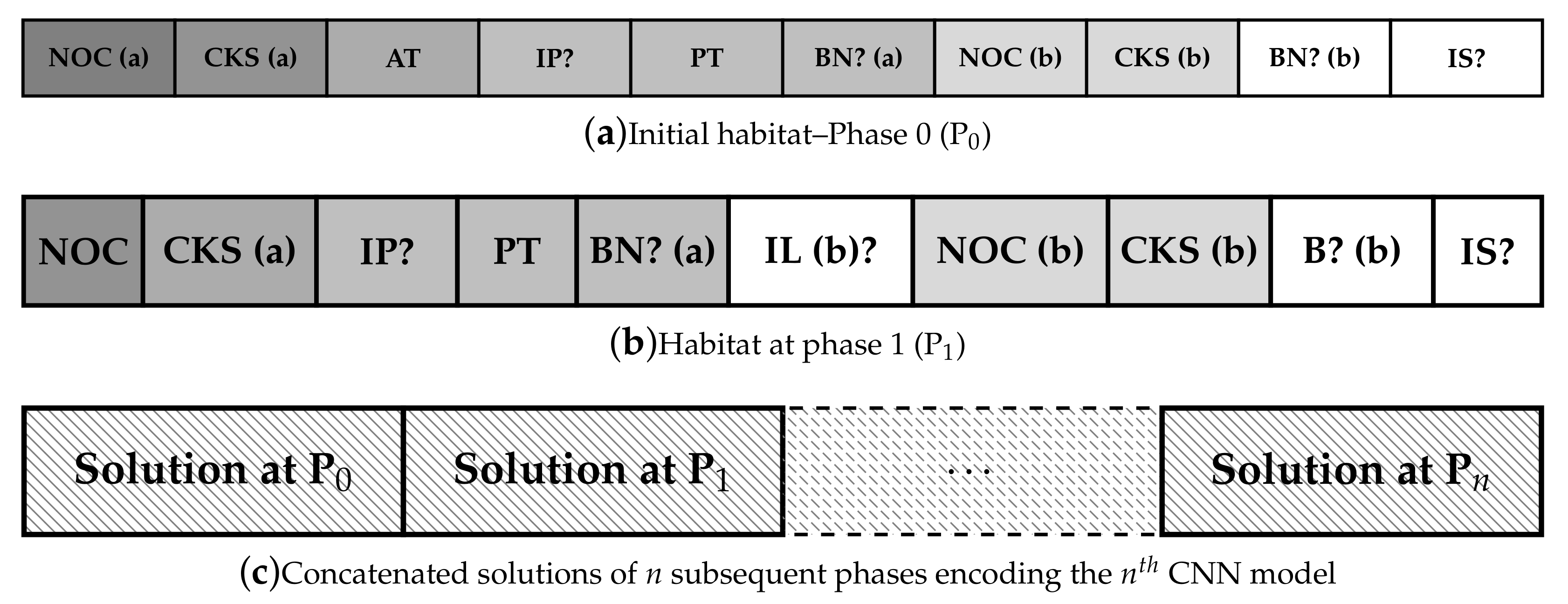
To represent networks as solutions in the search space, we use vectors containing the hyperparameters reported in Table 2. These are encoded according to the scheme depicted in Figure 3. As indicated in Section 2.2, we follow a given network type, but with variable hyperparameters such as the number of layers, number of neurons, pooling type, activation function type, number of Pooling Layer (PL), and so on. Each hyperparameter represent a design variable forming the candidate solution. If the first (randomly generated) CNN model does not pass the convergence test, a new “phase” is required. This consists of encoding new layers into candidate solutions and running a further optimisation round.
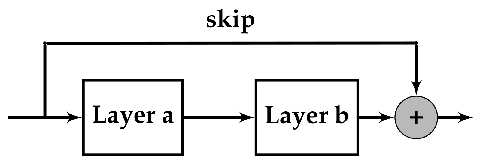
With reference to Figure 3, it can be seen that Phase 0 consists of the evolution of CNNs having two convolutional layers (i.e., layer a and layer b). In this initial phase, hyperparameters forming the design variables for the optimiation problem are the first six from Table 2, where NOC, CKS, and BN are used for layer a and b, giving ten parameters to emphasise. In all further phases, the parameters are those ten parameters except AT, but including IL, which determines if one or two layers are included. This gives ten parameters in every further phase. If a pooling layer is needed (PL = yes), this is be added after the first convolutional layer. If an skip connection is inserted (IS = yes), it must have a convolution. The skip connection structure is depicted in Figure 4.
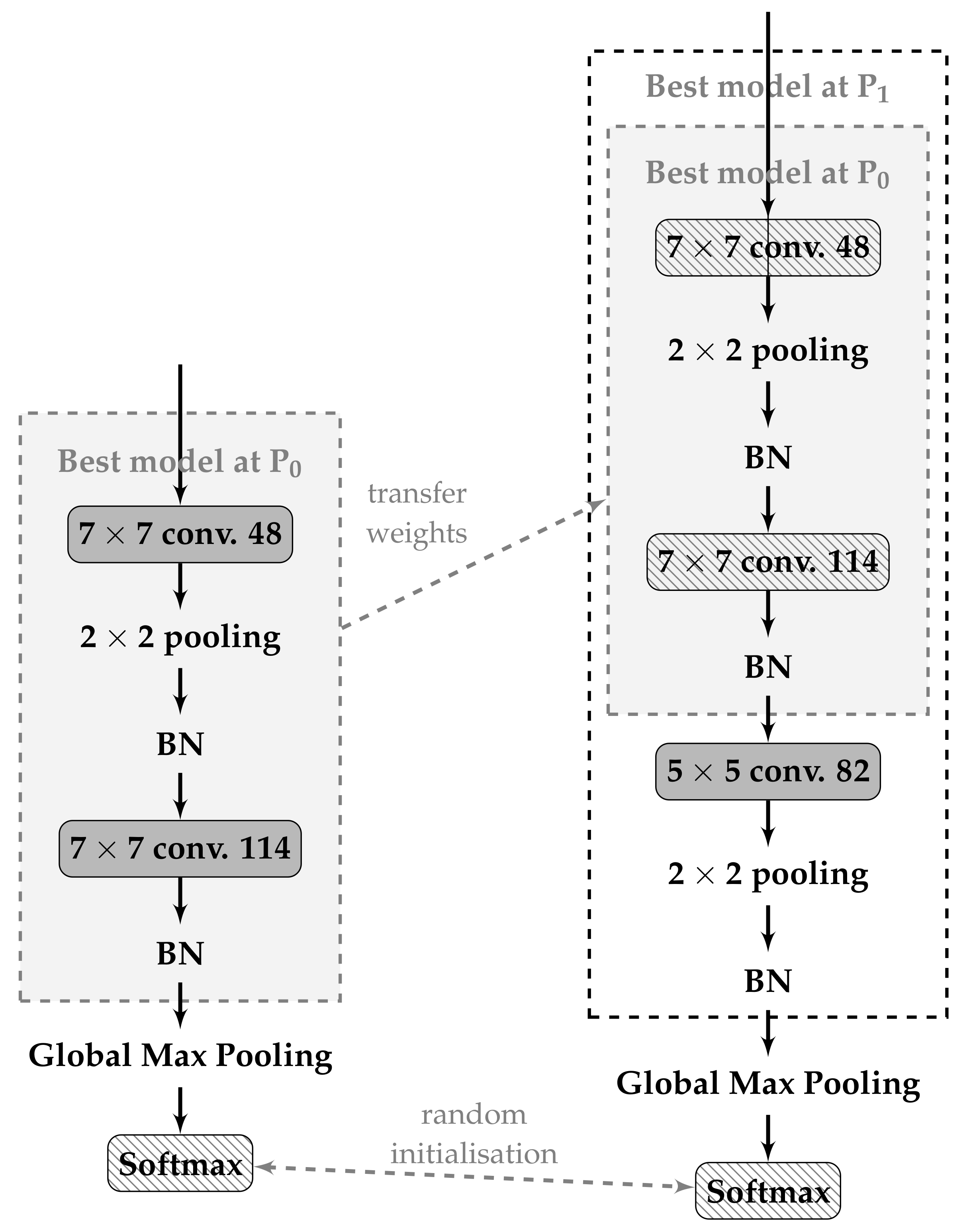
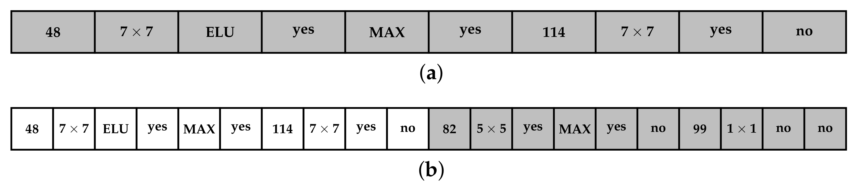
In subsequent phases, at most two additional convolutional layers (Layer a and Layer b) are added according to the scheme of Figure 3b (depicting Phase 1) and randomly initialised. The newly added parts follow a similar scheme to the one described for Phase 0. However, these lack the AT field and contain the “Include Layer b?” component. If the latter is active (i.e., its value is 1), this phase will use two convolution layers. Conversely, if its value is null, second layer will not be added. In both the cases, the CNN model grows gradually deeper. An example of this expansion process is displayed in Figure 5.
In this graphical representation, the best model obtained in Phase 0 is reported on the left-hand side. Note that the section inside the dashed box indicates the optimised part, while the last two blocks are added after the optimisation process to complete the CNN with the output node. To enter Phase 1, or any subsequent phase, the model obtained in the previous phase gets copied and the new additional layers added as previously explained to form the structure on the right-hand. The newly and deeper CNN models are therefore built up by stacking together optimised layers and adding new blocks that need to be optimised. Their optimisation is not completely independent to the previous optimisation processes as the fitness function can only be evaluated by considering the whole structure, and not only its parts. However, new candidate solutions are only formed by the new parameters. In other words, best solutions returned by BBO in subsequent phases need to be concatenated to encode the corresponding CNN. From the point of view of the network, this is equivalent to say that only the optimiser only works on the new layer while it grows. An example (referring to Phase 1) is shown in the right part of Figure 5. The gray section is inherited from Phase 0 while the remaining layers in the dashed box gets optimised. Figure 6 shows two example phases generating a network. This network has three convolutional layers, since IL? in the second phase is no, meaning we only add one more convolutional layer in the second phase. It also includes two pooling layers since IP? is yes for both phases.
It is worth noting that the encoding schemes described in this section generate two different search spaces with the size of the optimisation problem being 156,800 for the first phase, and 78,400 for each subsequent phase. These figures, obtained by timing the numbers of admissible values for the 10 design variables forming a candidate solution, indicate the maximum number of network configurations that each phase can generate. Hence, the proposed framework is capable of generating a vast number of network configurations by exploring a space of 156,800 + 78,400 cases over n phases.
3.2. Fitness Function Evaluation
As previously indicated, the accuracy obtained using the training and test data described in Section 2.1 is the fitness value assigned to the candidate solutions.
To obtain this value, the CNN encoded by a candidate solution is initialised (the two final modules shown in Figure 5 have to be attached) and trained to converge. Comparing the CNNs’ performance based on the test set is preferable, but not many epochs can be used due to time required to complete this process. However, when the number of epochs is low, deeper CNNs might have similar or even worse test accuracy than shallower ones. To overcome this problem, intelligent initialisation is a solution. This motivates our choice of embedding optimal results from previous parts into the network used in subsequent phases. This way, the dimensional of the problem does not change after the first phase (i.e., P) and the fitness fiction does not require several epochs to return a reliable accuracy measure. We noted that a CNN that is fitter in the initial training epochs tends to perform better also in the remaining epochs. This empirical observation let us fix a number of 5 epochs for the fitness evaluation.
3.3. Optimising the Layers
At most two layers need to be optimised by tuning the corresponding hyperparameters. This can be done with a metaheuristic algorithm that can handle discrete values. The BBO algorithm was employed because of the advantages indicated in Section 2.3, and returned satisfactory results. We empirically ruled out several configurations of the algorithm and eventually employed an elitist version where the fittest (i.e., CNNs with highest accuracy) solutions are always carried forward to the next generation. A similar approach was used for tuning the parameters of the BBO algorithm which confirmed the validity of the suggested setting in [51]. To achieve the highest possible accuracy, we do employ the mutation operator. The latter, is applied to individuals selected via the roulette-wheel selection method [34] where the probability are obtained with the original self-adaptive method in [51,59]. For the sake of clarity and applicability, the employed parameters setting is reported in Table 3. Note that BBO is run for 4000 iterations during each phase of the proposed framework.
3.4. Convergence Test
The evolving process terminates when there is no more significant enhancement (i.e., smaller than ) on validation accuracy while adding more layers. In other words, if the fitness of the best solution for a generic phase is , and the one the for the previous phase was such that , then we found an optimal structure and the network encoded with a chain of the best solutions obtained with the performed phases is returned.
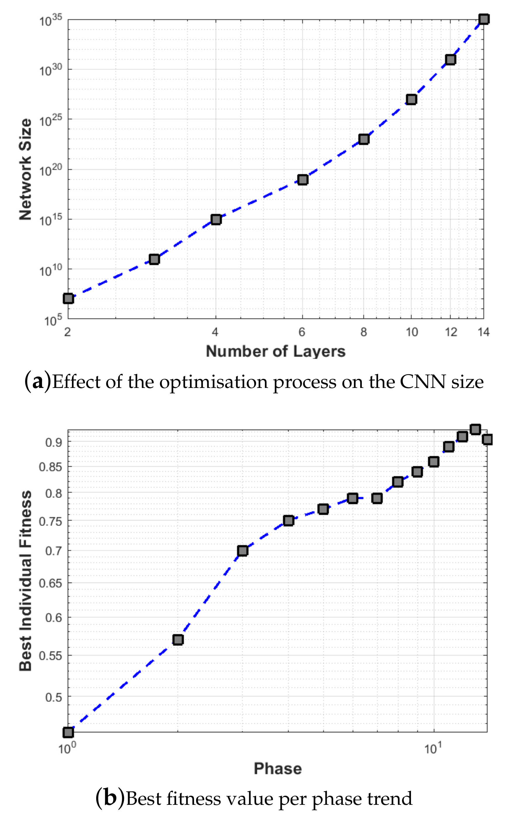
An example is available on Figure 7b, where the described process stops at the 15th phase with a best solution having a fitness value of . This is clearly show a significant deterioration of the performances given that the fitness function value at phase number 14 was , thus having .
4. Results
In this section, we describe the neural network ultimately designed by the system. The performance of this classifier is then evaluated based on accuracy and complexity for the COVID-19 problem and compared to benchmark methods in this field of study using three benchmark datasets. Finally, we use the Class Activation Mapping technique to find discriminative regions in the images.
4.1. The Final Neural Network
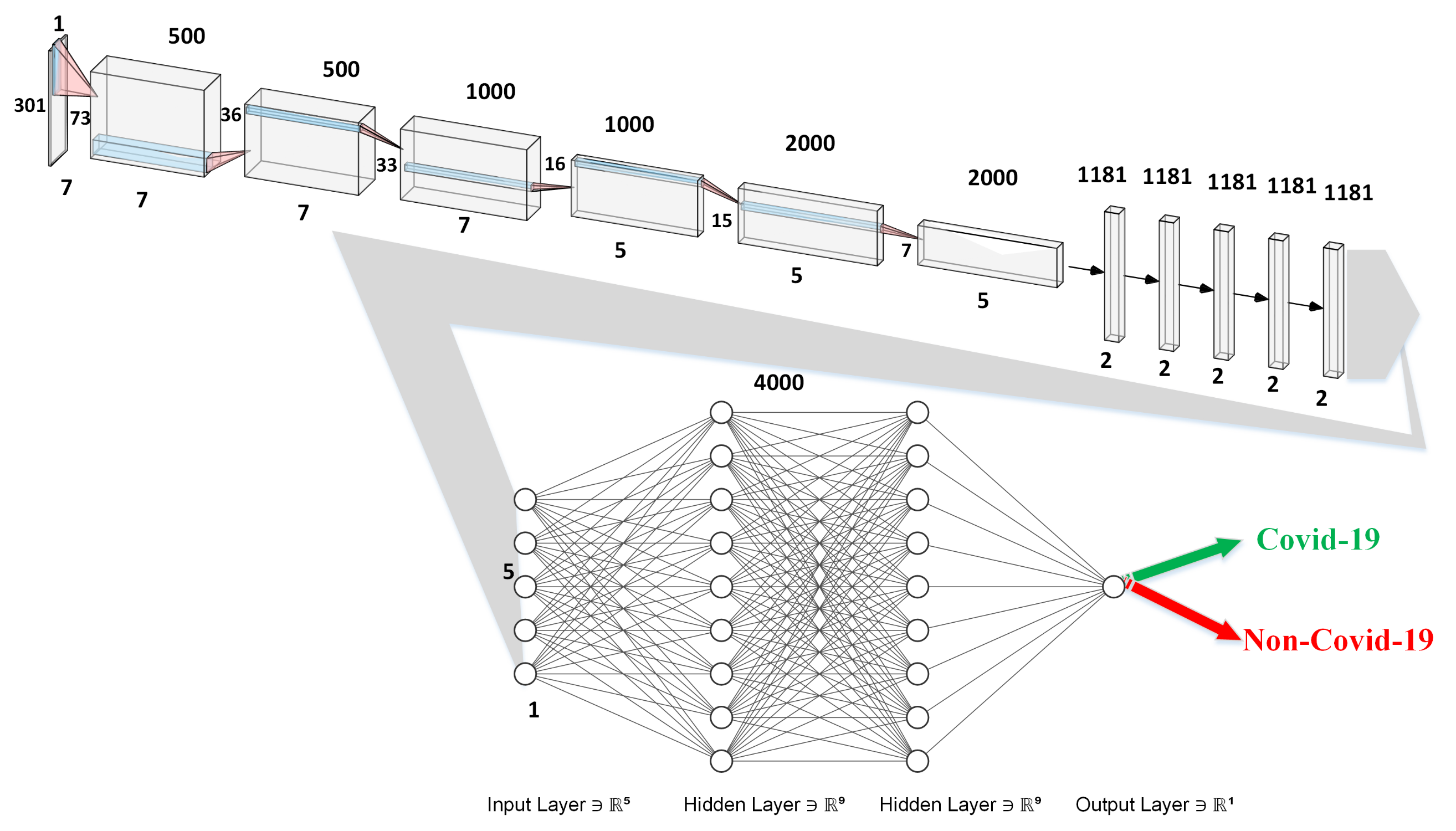
Then structure of the DCNN resulting from the optimisation process described before is shown in Figure 8. On the input greyscale image, 500 convolutions are carried out with a filter size of and a stride of , resulting in 500 grayscale images of pixels. Following this, a max-pooling is executed, with a stride, producing 500 images of pixels. This is followed by three convolutional with different filter sizes and one pooling layer, as reported in Table 4. After that, six extra convolutions are carried out, with the first five convolutions being padded, resulting in four thousand images. Finally, three layers of fully connected neurons are utilized, with four thousand, four thousand, and two neurons, respectively. The outcome value from the final layer is the probability of target and non-target.
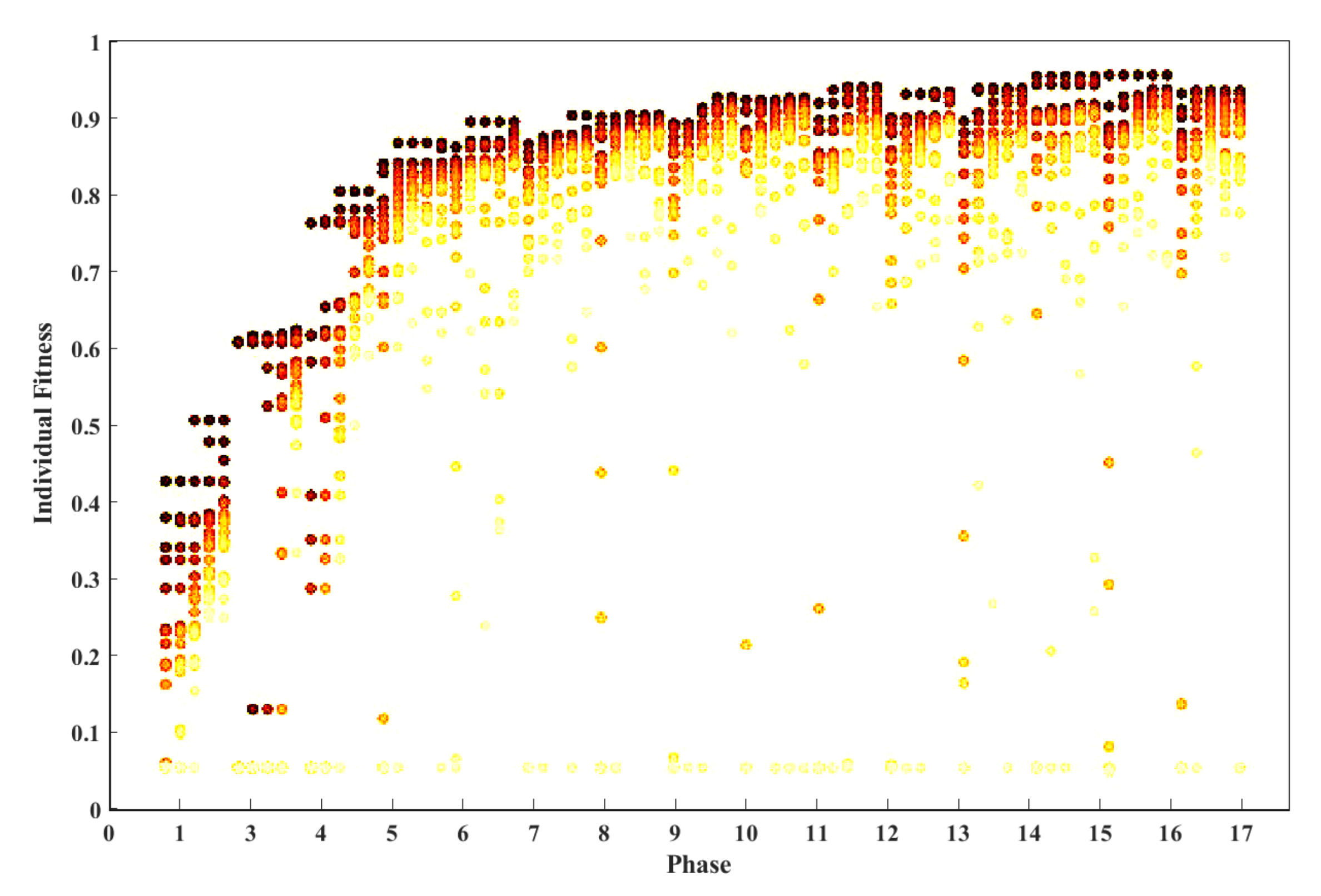
The optimisation of the architecture is shown in Figure 9, which plots the result of twenty candidate solutions developed gradually for five generations in each phase. Each corresponding network is trained for five epochs to obtain the fitness value. The evolution terminates at phase fifteen when the stopping criteria are satisfied. The number of convolutional layers increases in each phase. Initially, when the algorithm enters a new phase, there is a significant improvement in the candidate solutions’ accuracy. This improvement gradually declines in the later stages. This shows that the increase of convolutional layers can significantly influence the model performance, especially when the model is relatively shallow and too small to deal with the problem. As the number of layers increases, the network’s size grows, increasing the network’s capability.
4.2. Performance of the Designed Classifier
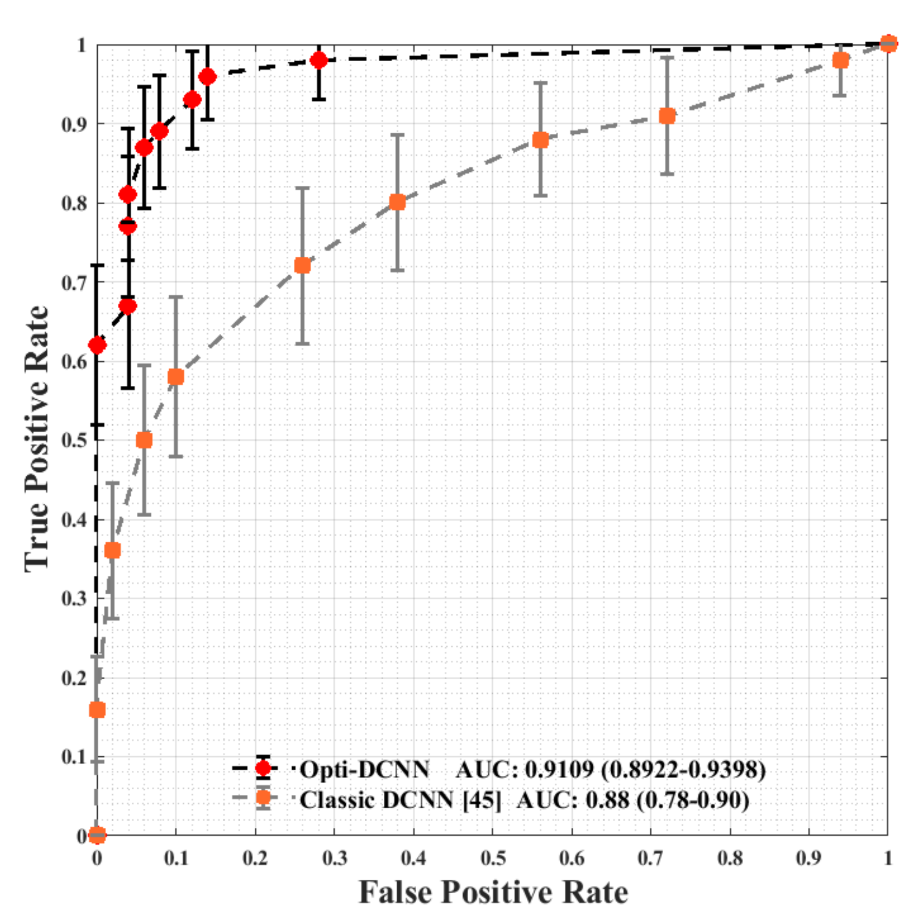
After training and validating the DCNN using the COVID X-ray-5k dataset, in this step, we test the trained DCNN using the COVID-X-ray-5k dataset. Since the accuracy rate alone does not give enough information about the classifier’s performance, Receiver Operating Characteristic (ROC) curves were calculated by exploiting the classifier on all the samples in the test dataset, thus producing a probability for each example. Afterward, a threshold value was introduced, and for each threshold value, the accuracy was calculated. The computed values were then plotted as a ROC curve. Generally, the area under the ROC plot indicates the probability of the correct classification. Figure 10 demonstrates the computed ROC curve for the classification of targets using OptiDCNN and classic DCNN. The ROC curves indicate that we significantly outperform classic DCNN on the test dataset.
The training was repeated ten times, resulting in training times betweeen five and eight minutes, and an accuracy of between 89.22% and 93.98% on the validation set. Due to the extensive range of accuracy values obtained, the ten trained OptiDCNNs are ensembled by weighted average, using the weights’ validation accuracy. The ensemble OptiDCNN achieves a validation accuracy of 91.09%, while DCNN had an accuracy of between 78% and 90%, and the resulting ensemble attained an accuracy of 88.3% on the validation dataset.
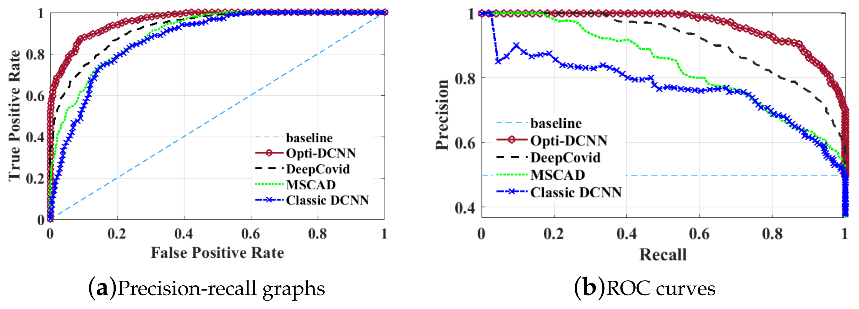
To further evaluate the OptiDCNN classifier’s performance, more testing data were produced by adding synthesized noise to the sample images. Figure 11 indicates the resulting ROC curve based on 2160 samples or ten various noisy realisations, using the algorithms OptiDCNN, classic DCNN, DeepCovid, and MSCAD. As shown in Figure 11, the OptiDCNN detector represents outstanding diagnostic results compared with other benchmark detection approaches. As a comparison, our proposed OptiDCNN provides over 93.5% diagnostic result with less than 6.5% false negative rate, which is an improvement over results reported by other benchmark classification approaches.
Generally speaking, the precision-recall curve indicates the tradeoff between recall and precision for various threshold levels. A high area under the precision-recall curve shows high precision and recall. High precision indicates a low false-positive rate, and high recall indicates a low false-negative rate. As can be observed from the curves in Figure 11, DCNN-ALHBBO has a higher area under the precision-recall curves. Therefore, it indicates a lower false positive and false negative rate than other benchmark classification approaches.
4.3. Comparison to Other Classifiers
The obtained accuracy for various classifiers is summarized in Table 5. The OptiDCNN is evaluated only once for each epoch because the accuracy does not change if the evaluation is repeated with the same experimental condition. In general, the tests conducted show that the higher the epoch value, the better is the accuracy. For example, in the first epoch, compared to DCNN (84.11%), the accuracy increased by 4.01% for MSCAD (88.12%), by 5.18% to OptiDCNN (89.2%9), and by 2.04% for DeepCovid (86.15%). While in the fifth epoch, compared to DCNN (93.47%), the increase in accuracy is 1.94% for MSCAD (95.41%), 4.09 for OptiDCNN (97.56%), and 0.50% for DeepCovid (93.97%). In the case of 10 epochs, as reported in Table 4, the increase in accuracy compared to DCNN (97.18%) is only 0.04 for MSCAD (97.22%), 2.67% for OptiDCNN (99.85%), and 0.28% for DeepCovid (97.46%).
4.4. Class Activation Mapping
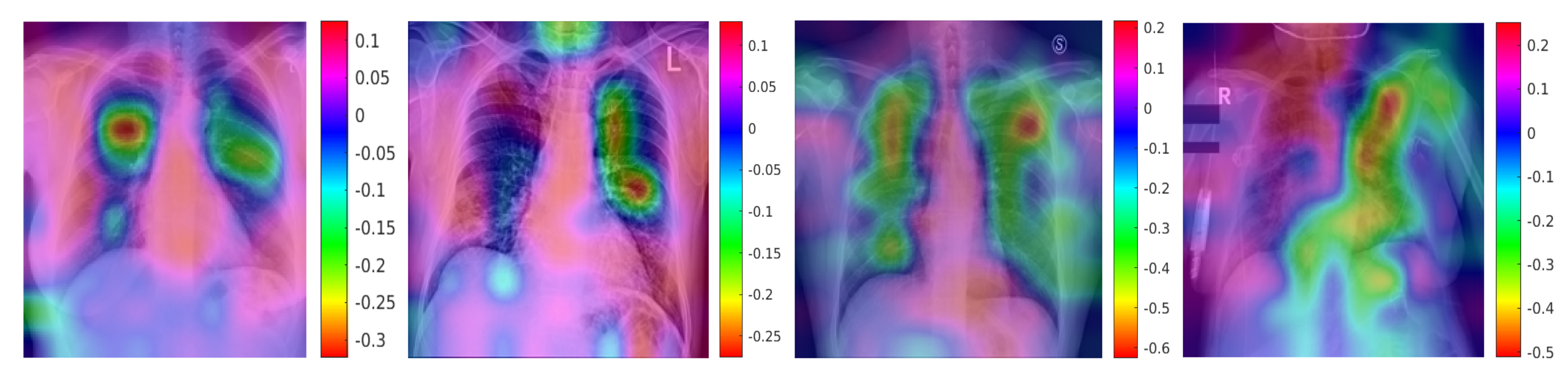
In addition to the accuracy of the classification, we also look at finding regions in the image which contribute to the classification. Class Activation Mapping (CAM) [39] is used for this. This maps the probability predicted by the DCNN model back to the last convolutional layer of the corresponding model to emphasize the discriminative regions, which are unique for each class.
The CAM for a determined image class is the outcome of the activation map of the Rectified Linear Unit (ReLU) layer following the last convolutional layer. It is identified by how much each activation mapping contributes to the final grade of that particular class. The novelty of CAM is the total average pooling layer applied after the last convolutional layer based on the spatial location to produce the connection weights. Thereby, it permits identifying the desired regions within an X-ray image that differentiates the class specificity preceding the softmax layer, which can enhance trust in the results.
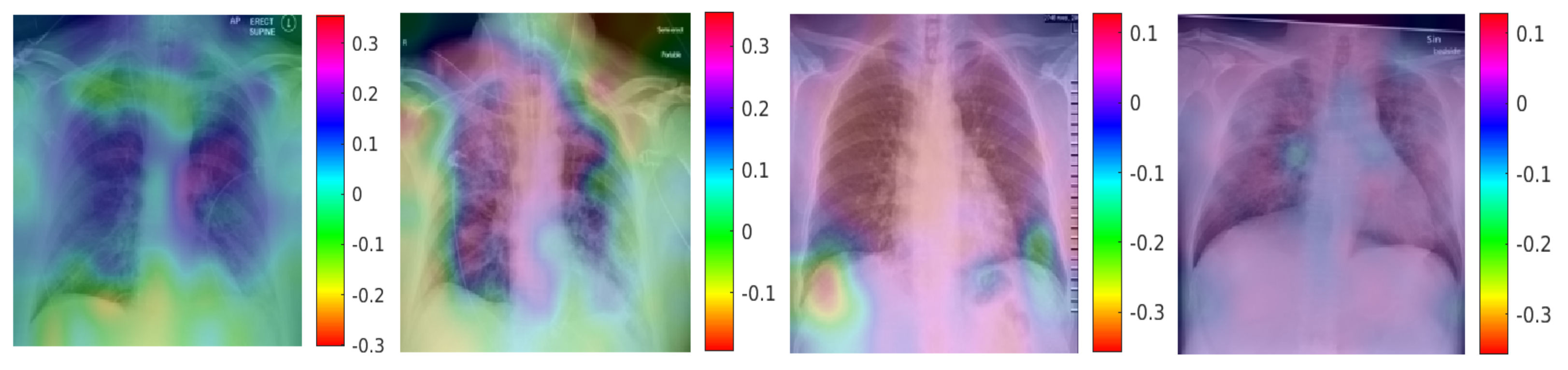
Figure 12 and Figure 13 show the discriminative regions for some X-ray images. Figure 12 shows the outcomes for the case marked as ‘Covid-19’ by the radiologist, Figure 13 shows the outcomes for a ‘normal’ case in Xray images. The OptiDCNN model predicts those cases correctly, and also indicates the discriminative area for its decision. Clearly, different regions are emphasised in the Covid-19 and the ‘normal’ cases. This shows that the network does a useful classification. In a next step, this kind of CAM visualisation can provide a useful second opinion to the medical specialists and radiology experts and improve their understanding of deep learning models.
5. Discussion
The network which is the result of the optimisation process shows a typical architecture for an image classification task. In so far the result is conforming the view that such a network is a good tool for the purpose. On the other hand, the exact number of layers, their order, and other hyperparameters are not obvious. For example, the use of pooling layers after the first and fifth convolutional layers only is quite specific and would probably not have been chosen manually.
Figure 9 shows how the network develops during the optimisation. It indicates the result of twenty habitats developing gradually for five generations in each phase. Each habitat is trained for five epochs to approximate the fitness function. The evolution terminates at phase fifteen when the stopping criteria are satisfied. The number of layers increases in each subsequent phase. As expected, when a new phase starts, the accuracy of the habitats improves significantly. This improvement in performance gradually decreases in the later stages. This shows that the increase of layers can have a significant effect on the performance of DCNNs, mainly when CNN is relatively shallow. The evolution clearly shows that our network is a near optimal network for the purpose.
We have also shown that our network performs better than other classification approaches. In order to clearly establish the superiority of our network, we have used different numbers of epochs for training. The results (Table 5) indicate that OptiDCNN represents the best accuracy for all epochs. Accuracy improvement of OptiDCNN, compared to the original DCNN, varies for each epoch, with a range of values between (the tenth epoch) up to (the first epoch). OptiDCNN is also faster than other approaches, as shown in Table 6. The computation time for OptiDCNN, compared to the classic DCNN, is in the range of 97% (for the first epoch: 99.11/102.11) down to 82% times (for the tenth epoch: 934.54/1133.44). It is evident that as the number of epoch increases, the time efficiency of the ALHBBO is more prominent because the adaptive length of the BBO algorithm leads to decreasing the complexity of the search space.
Achieving a good result with respect to accuracy, precision, or other parameters is crucial for solving the problem. In practice, domain specialists, in our case medical specialists and radiologists, tend to be sceptical if result cannot be interpreted and justified. We have therefore used Class Activation Mapping to provide more information about individual instances. Since we can reliably identify critical regions in the scans, the network’s decision-making can enhance the understanding of both medical specialists and data science experts. This is a step towards explainable AI, a current topic in research and application.
6. Conclusions
In this paper, OptiDCNN was proposed to design an accurate DCNN model for positive Covid-19 X-ray detection. The designed detector was benchmarked on the COVID-Xray-5k dataset, and the results were evaluated by a comparative study with classic DCNN, DeepCovid, and MSCAD. The results indicated that the designed detector is able to present very competitive results compared to these benchmark models. The concept of CAM was also applied to detect the virus’s regions potentially infected. It was found to correlate with clinical results, as confirmed by experts. A few research directions can be proposed for future work with the OptiDCNN, such as underwater sonar target detection and classification. These application domains might different kind of heuristics to tackle multi-objective optimisation problems. The investigation of the chaotic maps’ effectiveness to improve the performance of the OptiDCNN can be another research direction. Although the results are promising, further study is needed on a larger dataset of COVID-19 images to have a more comprehensive evaluation of accuracy rates. Another interesting issue for further exploration is the use of light or difficult to detect cases, since we have restricted ourselves to clear cases. Further research should explore how the existing network works on those cases and how it can be emphasised for them. Finally, to further improve upon the proposed method, we envisage exploring different optimisation approaches and validation methods for our model. As we obtained promising results by simply selecting validation and training images at random, a worth trying approach would be the “repeated random sub-sampling validation”, also known as Monte Carlo cross-validation [60].
Author Contributions
Conceptualization, all; methodology, M.K.; software, M.K.; validation, F.C., S.K.; formal analysis, all; investigation, all; writing—original draft, M.K., F.C. and S.K.; writing—review and editing, F.C., S.K.; visualisation, M.K., F.C. All authors have read and agreed to the published version of the manuscript.
Funding
This research received no external funding.
Informed Consent Statement
Not applicable.
Conflicts of Interest
The authors declare no conflict of interest.
References
- Gabutti, G.; d’Anchera, E.; Sandri, F.; Savio, M.; Stefanati, A. Coronavirus: Update Related to the Current Outbreak of COVID-19. Infect. Dis. Ther. 2020, 9, 241–253. [Google Scholar] [CrossRef]
- WHO. What’s New in the Guidelines. 2021. Available online: https://www.covid19treatmentguidelines.nih.gov/whats-new/ (accessed on 3 February 2021).
- Ün, M.K.; Avşar, E.; Akçalı, İ.D. An analytical method to create patient-specific deformed bone models using X-ray images and a healthy bone model. Comput. Biol. Med. 2019, 104, 43–51. [Google Scholar] [CrossRef]
- Toğaçar, M.; Ergen, B.; Cömert, Z. COVID-19 detection using deep learning models to exploit Social Mimic Optimization and structured chest X-ray images using fuzzy color and stacking approaches. Comput. Biol. Med. 2020, 121, 103805. [Google Scholar] [CrossRef]
- García-Ruesgas, L.; Álvarez Cuervo, R.; Valderrama-Gual, F.; Rojas-Sola, J.I. Projective geometric model for automatic determination of X-ray-emitting source of a standard radiographic system. Comput. Biol. Med. 2018, 99, 209–220. [Google Scholar] [CrossRef]
- Kengyelics, S.M.; Treadgold, L.A.; Davies, A.G. X-ray system simulation software tools for radiology and radiography education. Comput. Biol. Med. 2018, 93, 175–183. [Google Scholar] [CrossRef] [Green Version]
- Bielby, J.; Kuhn, S.; Colreavy-Donnelly, S.; Caraffini, F.; O’Connor, S.; Anastassi, Z.A. Identifying Parkinson’s Disease through the Classification of Audio Recording Data. In Proceedings of the 2020 IEEE Congress on Evolutionary Computation (CEC), Glasgow, UK, 19–24 July 2020; pp. 1–7. [Google Scholar] [CrossRef]
- Santucci, V.; Milani, A.; Caraffini, F. An Optimisation-Driven Prediction Method for Automated Diagnosis and Prognosis. Mathematics 2019, 7, 1051. [Google Scholar] [CrossRef] [Green Version]
- Thurnhofer-Hemsi, K.; López-Rubio, E.; Roe-Vellve, N.; Molina-Cabello, M.A. Multiobjective optimization of deep neural networks with combinations of Lp-norm cost functions for 3D medical image super-resolution. Integr. Comput. Aided Eng. 2020, 27, 233–251. [Google Scholar] [CrossRef]
- Charte, F.; Rivera, A.J.; Martínez, F.; del Jesus, M.J. EvoAAA: An evolutionary methodology for automated neural autoencoder architecture search. Integr. Comput. Aided Eng. 2020, 27, 211–231. [Google Scholar] [CrossRef]
- Togo, R.; Watanabe, H.; Ogawa, T.; Haseyama, M. Deep convolutional neural network-based anomaly detection for organ classification in gastric X-ray examination. Comput. Biol. Med. 2020, 123, 103903. [Google Scholar] [CrossRef]
- Colreavy-Donnelly, S.; Caraffini, F.; Kuhn, S.; Gongora, M.; Florez-Lozano, J.; Parra, C. Shallow buried improvised explosive device detection via convolutional neural networks. Integr. Comput. Aided Eng. 2020, 27, 403–416. [Google Scholar] [CrossRef]
- Bonet, I.; Caraffini, F.; Peña, A.; Puerta, A.; Gongora, M. Oil Palm Detection via Deep Transfer Learning. In Proceedings of the 2020 IEEE Congress on Evolutionary Computation (CEC), Glasgow, UK, 19–24 July 2020; pp. 1–8. [Google Scholar] [CrossRef]
- Gasienica-Józkowy, J.; Knapik, M.; Cyganek, B. An ensemble deep learning method with optimized weights for drone-based water rescue and surveillance. Integr. Comput. Aided Eng. 2021. [Google Scholar] [CrossRef]
- Hamreras, S.; Boucheham, B.; Molina-Cabello, M.A.; Benitez-Rochel, R.; Lopez-Rubio, E. Content based image retrieval by ensembles of deep learning object classifiers. Integr. Comput. Aided Eng. 2020, 27, 317–331. [Google Scholar] [CrossRef]
- Mahmud, T.; Rahman, M.A.; Fattah, S.A. CovXNet: A multi-dilation convolutional neural network for automatic COVID-19 and other pneumonia detection from chest X-ray images with transferable multi-receptive feature optimization. Comput. Biol. Med. 2020, 122, 103869. [Google Scholar] [CrossRef]
- Ozturk, T.; Talo, M.; Yildirim, E.A.; Baloglu, U.B.; Yildirim, O.; Rajendra Acharya, U. Automated detection of COVID-19 cases using deep neural networks with X-ray images. Comput. Biol. Med. 2020, 121, 103792. [Google Scholar] [CrossRef]
- Panwar, H.; Gupta, P.; Siddiqui, M.K.; Morales-Menendez, R.; Singh, V. Application of deep learning for fast detection of COVID-19 in X-Rays using nCOVnet. Chaos Solitons Fractals 2020, 138, 109944. [Google Scholar] [CrossRef]
- Apostolopoulos, I.D.; Mpesiana, T.A. Covid-19: Automatic detection from X-ray images utilizing transfer learning with convolutional neural networks. Phys. Eng. Sci. Med. 2020, 43, 635–640. [Google Scholar] [CrossRef] [PubMed] [Green Version]
- Aggarwal, C.C. Neural Networks and Deep Learning. A Textbook; Springer International: Cham, Switzerland, 2018. [Google Scholar]
- Yun, K.; Huyen, A.; Lu, T. Deep Neural Networks for Pattern Recognition. arXiv 2018, arXiv:1809.09645. [Google Scholar]
- Le, Q.V.; Ngiam, J.; Coates, A.; Lahiri, A.; Prochnow, B.; Ng, A.Y. On Optimization Methods for Deep Learning. In Proceedings of the 28th International Conference on International Conference on Machine Learning, Bellevue, WA, USA, 28–2 July 2011; Omnipress: Madison, WI, USA, 2011; pp. 265–272. [Google Scholar]
- Arulkumaran, K.; Deisenroth, M.P.; Brundage, M.; Bharath, A.A. Deep Reinforcement Learning: A Brief Survey. IEEE Signal Process. Mag. 2017, 34, 26–38. [Google Scholar] [CrossRef] [Green Version]
- Vinyals, O.; Povey, D. Krylov Subspace Descent for Deep Learning. In Proceedings of the Fifteenth International Conference on Artificial Intelligence and Statistics, La Palma, Spain, 21–23 April 2012; Lawrence, N.D., Girolami, M., Eds.; PMLR: La Palma, Spain, 2012; Volume 22, pp. 1261–1268. [Google Scholar]
- Olshanskii, M.A.; Tyrtyshnikov, E.E. Krylov Subspace Methods. In Iterative Methods for Linear Systems: Theory and Applications; Society for Industrial and Applied Mathematics: Philadelphia, PA, USA, 2014; pp. 1–65. [Google Scholar] [CrossRef]
- Kawaguchi, K. Deep Learning without Poor Local Minima. In Proceedings of the 29th International Conference on Neural Information Processing Systems, Montreal, QC, Canada, 5–10 December 2015; pp. 586–594. [Google Scholar]
- Sutskever, I.; Martens, J.; Dahl, G.; Hinton, G. On the importance of initialization and momentum in deep learning. In Proceedings of the 30th International Conference on Machine Learning, Atlanta, GA, USA, 16–21 June 2013; Dasgupta, S., McAllester, D., Eds.; PMLR: Atlanta, GA, USA, 2013; Volume 28, pp. 1139–1147. [Google Scholar]
- Hu, K.; Jiang, H.; Ji, C.G.; Pan, Z. A modified butterfly optimization algorithm: An adaptive algorithm for global optimization and the support vector machine. Expert Syst. 2020, 38, e12642. [Google Scholar] [CrossRef]
- Yeoh, J.M.; Caraffini, F.; Homapour, E.; Santucci, V.; Milani, A. A Clustering System for Dynamic Data Streams Based on Metaheuristic Optimisation. Mathematics 2019, 7, 1229. [Google Scholar] [CrossRef] [Green Version]
- Demirel, D.; Cetinsaya, B.; Halic, T.; Kockara, S.; Ahmadi, S. Partition-based optimization model for generative anatomy modeling language (POM-GAML). BMC Bioinform. 2019, 20, 105. [Google Scholar] [CrossRef]
- Cho, M.; Dhir, C.S.; Lee, J. Hessian-Free Optimization for Learning Deep Multidimensional Recurrent Neural Networks. In Proceedings of the 28th International Conference on Neural Information Processing Systems, Montreal, Canada, 18–23 December 2014; pp. 883–891. [Google Scholar]
- Florez-Lozano, J.; Caraffini, F.; Parra, C.; Gongora, M. Cooperative and distributed decision-making in a multi-agent perception system for improvised land mines detection. Inf. Fusion 2020, 64, 32–49. [Google Scholar] [CrossRef]
- Khishe, M.; Mosavi, M. Classification of underwater acoustical dataset using neural network trained by Chimp Optimization Algorithm. Appl. Acoust. 2020, 157, 107005. [Google Scholar] [CrossRef]
- Eiben, A.E.; Smith, J.E. Introduction to Evolutionary Computation; Springer: Berlin, Germany, 2003. [Google Scholar] [CrossRef]
- Stanley, K.O.; Clune, J.; Lehman, J.; Miikkulainen, R. Designing neural networks through neuroevolution. Nat. Mach. Intell. 2019, 1, 24–35. [Google Scholar] [CrossRef]
- Lee, W.Y.; Park, S.M.; Sim, K.B. Optimal hyperparameter tuning of convolutional neural networks based on the parameter-setting-free harmony search algorithm. Optik 2018, 172, 359–367. [Google Scholar] [CrossRef]
- Rosa, G.; Papa, J.; Marana, A.; Scheirer, W.; Cox, D. Fine-Tuning Convolutional Neural Networks Using Harmony Search. In Progress in Pattern Recognition, Image Analysis, Computer Vision, and Applications; Pardo, A., Kittler, J., Eds.; Springer International Publishing: Cham, Switzerland, 2015; pp. 683–690. [Google Scholar]
- Bąk, S.; Carr, P.; Lalonde, J.F. Domain Adaptation Through Synthesis for Unsupervised Person Re-identification. In Proceedings of the Computer Vision–ECCV 2018, Munich, Germany, 8–14 September 2018; Ferrari, V., Hebert, M., Sminchisescu, C., Weiss, Y., Eds.; Springer International Publishing: Cham, Switzerland, 2018; pp. 193–209. [Google Scholar]
- Fan, H.; Zheng, L.; Yan, C.; Yang, Y. Unsupervised Person Re-Identification: Clustering and Fine-Tuning. ACM Trans. Multimed. Comput. Commun. Appl. 2018, 14. [Google Scholar] [CrossRef]
- Qian, X.; Fu, Y.; Xiang, T.; Wang, W.; Qiu, J.; Wu, Y.; Jiang, Y.G.; Xue, X. Pose-Normalized Image Generation for Person Re-identification. In Proceedings of the Computer Vision–ECCV 2018, Munich, Germany, 8–14 September 2018; Ferrari, V., Hebert, M., Sminchisescu, C., Weiss, Y., Eds.; Springer International Publishing: Cham, Switzerland, 2018; pp. 661–678. [Google Scholar]
- Sun, Y.; Xue, B.; Zhang, M.; Yen, G.G.; Lv, J. Automatically Designing CNN Architectures Using the Genetic Algorithm for Image Classification. IEEE Trans. Cybern. 2020, 50, 3840–3854. [Google Scholar] [CrossRef] [PubMed] [Green Version]
- Young, S.R.; Rose, D.C.; Karnowski, T.P.; Lim, S.H.; Patton, R.M. Optimizing Deep Learning Hyper-Parameters through an Evolutionary Algorithm. In Proceedings of the Workshop on Machine Learning in High-Performance Computing Environments; Association for Computing Machinery: New York, NY, USA, 2015. [Google Scholar] [CrossRef]
- Real, E.; Moore, S.; Selle, A.; Saxena, S.; Suematsu, Y.L.; Tan, J.; Le, Q.V.; Kurakin, A. Large-Scale Evolution of Image Classifiers. In Proceedings of the 34th International Conference on Machine Learning, Sydney, Australia, 6–11 August 2017; Volume 70, pp. 2902–2911. [Google Scholar]
- Cohen, J.P.; Morrison, P.; Dao, L. COVID-19 Image Data Collection. arXiv 2020, arXiv:eess.IV/2003.11597. [Google Scholar]
- Minaee, S.; Kafieh, R.; Sonka, M.; Yazdani, S.; Soufi, G.J. Deep-covid: Predicting covid-19 from chest X-ray images using deep transfer learning. arXiv 2020, arXiv:2004.09363. [Google Scholar] [CrossRef]
- Irvin, J.; Rajpurkar, P.; Ko, M.; Yu, Y.; Ciurea-Ilcus, S.; Chute, C.; Marklund, H.; Haghgoo, B.; Ball, R.; Shpanskaya, K.; et al. Chexpert: A large chest radiograph dataset with uncertainty labels and expert comparison. Proc. AAAI Conf. Artif. Intell. 2019, 33, 590–597. [Google Scholar] [CrossRef]
- Voulodimos, A.; Doulamis, N.; Doulamis, A.; Protopapadakis, E. Deep Learning for Computer Vision: A Brief Review. Comput. Intell. Neurosci. 2018, 2018, 7068349. [Google Scholar] [CrossRef]
- Berg, H.; Hjelmervik, K.T. Classification of anti-submarine warfare sonar targets using a deep neural network. In Proceedings of the OCEANS 2018 MTS/IEEE Charleston, Charleston, SC, USA, 22–25 October 2018; pp. 1–5. [Google Scholar] [CrossRef]
- Rodríguez, A.; Tabassum, A.; Cui, J.; Xie, J.; Ho, J.; Agarwal, P.; Adhikari, B.; Prakash, B.A. DeepCOVID: An Operational Deep Learning-driven Framework for Explainable Real-time COVID-19 Forecasting. medRxiv 2020. [Google Scholar] [CrossRef]
- Hall, J.J.; Azimi-Sadjadi, M.R.; Kargl, S.G.; Zhao, Y.; Williams, K.L. Underwater Unexploded Ordnance (UXO) Classification Using a Matched Subspace Classifier With Adaptive Dictionaries. IEEE J. Ocean. Eng. 2019, 44, 739–752. [Google Scholar] [CrossRef]
- Simon, D. Biogeography-Based Optimization. IEEE Trans. Evol. Comput. 2008, 12, 702–713. [Google Scholar] [CrossRef] [Green Version]
- Kennedy, J. Swarm Intelligence. In Handbook of Nature-Inspired and Innovative Computing: Integrating Classical Models with Emerging Technologies; Zomaya, A.Y., Ed.; Springer: Boston, MA, USA, 2006; pp. 187–219. [Google Scholar] [CrossRef]
- Caraffini, F.; Santucci, V.; Milani, A. Evolutionary Computation & Swarm Intelligence; MDPI: Basel, Switzerland, 2020. [Google Scholar]
- Yaman, A.; Iacca, G.; Caraffini, F. A comparison of three differential evolution strategies in terms of early convergence with different population sizes. In LeGO 2018–14th International Global Optimization Workshop; AIP Publishing: Melville, NY, USA, 2019; p. 020002. [Google Scholar]
- Mirjalili, S.; Mirjalili, S.M.; Lewis, A. Let a biogeography-based optimizer train your multi-layer perceptron. Inf. Sci. 2014, 269, 188–209. [Google Scholar] [CrossRef]
- Hanski, I. Metapopulation dynamics. Nature 1998, 396, 41–49. [Google Scholar] [CrossRef]
- Hastings, A.; Higgins, K. Persistence of transients in spatially structured ecological models. Science 1994, 263, 1133–1136. [Google Scholar] [CrossRef]
- Ma, H. An analysis of the equilibrium of migration models for biogeography-based optimization. Inf. Sci. 2010, 180, 3444–3464. [Google Scholar] [CrossRef]
- Simon, D. Biogeography-Based Optimization. 2009. Available online: https://academic.csuohio.edu/simond/bbo/ (accessed on 27 April 2021).
- Xu, Q.S.; Liang, Y.Z. Monte Carlo cross validation. Chemom. Intell. Lab. Syst. 2001, 56, 1–11. [Google Scholar] [CrossRef]
Figure 1.
Six random sample images from the COVID-X-ray-5k dataset.

Figure 2.
A schematic overview of the evolutionary framework.

Figure 3.
Encoding of the neural networks during the various phases. In phase 0, there are two convolutional layers, called (a,b). For the abbreviations, see Table 2. In phase 1 and subsequent phases, which are identical, the activation type is no longer changed (therefore no AT in those phases), but it can be decided if a second layer is included (IL?). The concatenation of the phases is shown in subfigure (c). Yes/no hyperparameters are shown with a?

Figure 4.
An example of a skip connection.

Figure 5.
CNN grows deeper when a new phase begins (Left: Phase 0, right: Phase 1).

Figure 6.
Building deeper CNNs by concatenating solutions from performed phases. (a) An example of solution for P encoding the phase 0 CNN of Figure 5 (left), (b) Solutions at P and P encoding the phase 1 CNN of Figure 5 (right).

Figure 7.
The resulting expansion process. In (a) the size of the CNN increases as the number of its layers grows during the 15 performed phases. In (b) we show the optimisation process. The decreasing trend at the last 15th phase graphically indicates that the termination criterion (Section 3.4) is met.

Figure 8.
The topology of designed OptiDCNN. The number below of each box indicates the size of the outcome images, while the one above each box the number of filters used.
Figure 8.
The topology of designed OptiDCNN. The number below of each box indicates the size of the outcome images, while the one above each box the number of filters used.

Figure 9.
Fitness functions of the 20 fittest solutions returned after each performed phase. For illustration purposes, 17 phases are reported to show the validity of the proposed stopping criterion. Indeed, note that the accuracy slightly decreases after phase 15, i.e., layers added at phases 15, 16 and 17 are not needed.

Figure 10.
TPR curves for OptiDCNN and classic DCNN. The bars indicate the range of the ten runs performed.
Figure 10.
TPR curves for OptiDCNN and classic DCNN. The bars indicate the range of the ten runs performed.

Figure 11.
TPR/FPR graphs (a) and ROC curves (b) for OptiDCNN and other benchmark classifiers.

Figure 12.
ROI for positive Covid-19 cases using ACM.

Figure 13.
ROI for Normal cases using ACM.


Table 1.
Summary of the employed dataset.
| Category | COVID-19 | Healthy |
|---|---|---|
| Training Set | 84 (420 after augmentation) | 2000 |
| Test Set | 100 | 3000 |
Table 2.
Hyperparameters emphasised during the evolution of the network.
| Name | Acronym | Admissible Values |
|---|---|---|
| Number of Output Channels | NOC | 8, 16, 32, |
| 64, 128, 256, 512 | ||
| Convolution Kernel Size | CKS | , , |
| , , | ||
| Activation Type | AT | ReLU, Tanh |
| ELU, SELU | ||
| Include Pool | IP | Yes, No |
| Pooling Type | PT | Max pooling, |
| Average pooling | ||
| Batch Normalization | BN | Yes, No |
| Insert Skip | IS | Yes, No |
| Insert Layer | IL | Yes, No |
Table 3.
Employed parameters setting for BBO.
| Max immigration (I) | 1 |
| Max emigration (E) | 1 |
| Max mutation rate (M) | 0.02 |
Table 4.
The details of layers used in the designed DCNN.
| Layer | Type | No. Filters | Size | Stride | Resulting Dimension |
|---|---|---|---|---|---|
| 1 | Convolution | 500 | |||
| 2 | Pooling | 500 | |||
| 3 | Convolution | 1000 | |||
| 4 | Convolution | 1000 | |||
| 5 | Convolution | 2000 | |||
| 6 | Pooling | 2000 | |||
| 7 | Convolution (padded) | 1181 | |||
| 8 | Convolution (padded) | 1181 | |||
| 9 | Convolution (padded) | 1181 | |||
| 10 | Convolution (padded) | 1181 | |||
| 11 | Convolution (padded) | 1181 | |||
| 12 | Convolution | 4000 | |||
| 13 | Fully connected (4000 nodes) | ||||
| 14 | Dropout (probability = ) | ||||
| 15 | Fully connected (4000 nodes) | ||||
| 16 | Dropout (probability = ) | ||||
| 17 | Fully connected (2 nodes) |
Table 5.
Accuracy and standard deviation ‘STD’ for benchmark networks.
| Epoch | OptiDCNN | MSCAD | DeepCovid | DCNN | ||||
|---|---|---|---|---|---|---|---|---|
| Accuracy | STD | Accuracy | STD | Accuracy | STD | Accuracy | STD | |
| 1 | 89.63 | N/A | 88.12 | 0.41 | 87.26 | 0.33 | 84.11 | 0.75 |
| 2 | 93.11 | N/A | 92.11 | 0.37 | 91.33 | 0.21 | 89.22 | 0.31 |
| 3 | 96.15 | N/A | 93.12 | 0.31 | 92.09 | 0.22 | 91.11 | 0.38 |
| 4 | 97.22 | N/A | 94.62 | 0.24 | 92.89 | 0.32 | 92.47 | 0.11 |
| 5 | 97.27 | N/A | 95.41 | 0.18 | 93.55 | 0.09 | 93.47 | 0.29 |
| 6 | 98.41 | N/A | 95.92 | 0.17 | 95.25 | 0.18 | 94.02 | 0.39 |
| 7 | 98.55 | N/A | 96.11 | 0.16 | 96.13 | 0.19 | 95.17 | 0.19 |
| 8 | 98.88 | N/A | 96.77 | 0.12 | 97.24 | 0.11 | 96.58 | 0.21 |
| 9 | 99.01 | N/A | 96.99 | 0.09 | 98.11 | 0.15 | 96.76 | 0.09 |
| 10 | 99.11 | N/A | 97.22 | 0.15 | 98.22 | 0.09 | 97.18 | 0.11 |
Table 6.
Computation time (in seconds) and STD for benchmark networks.
| Epoch | OptiDCNN | MSCAD | DeepCovid | DCNN | ||||
|---|---|---|---|---|---|---|---|---|
| Time | STD | Time | STD | Time | STD | Time | STD | |
| 1 | 99.11 | N/A | 102.23 | 1.01 | 102.08 | 0.89 | 102.11 | 0.77 |
| 2 | 201.04 | N/A | 236.03 | 8.54 | 255.11 | 1.54 | 268.47 | 4.33 |
| 3 | 302.62 | N/A | 347.41 | 2.32 | 387.55 | 2.28 | 299.17 | 0.53 |
| 4 | 355.13 | N/A | 421.45 | 2.01 | 521.27 | 2.18 | 443.49 | 0.65 |
| 5 | 461.11 | N/A | 582.47 | 3.96 | 533.26 | 1.32 | 601.77 | 3.09 |
| 6 | 555.22 | N/A | 692.75 | 1.23 | 611.75 | 5.96 | 721.22 | 2.01 |
| 7 | 645.39 | N/A | 797.02 | 1.02 | 725.68 | 4.15 | 836.75 | 2.25 |
| 8 | 747.55 | N/A | 854.43 | 1.74 | 805.74 | 4.02 | 1007.9 | 1.53 |
| 9 | 875.35 | N/A | 964.12 | 2.01 | 953.89 | 6.05 | 1125.57 | 5.07 |
| 10 | 934.54 | N/A | 1112.36 | 1.97 | 1211.34 | 1.33 | 1133.44 | 4.25 |
Publisher’s Note: MDPI stays neutral with regard to jurisdictional claims in published maps and institutional affiliations. |
© 2021 by the authors. Licensee MDPI, Basel, Switzerland. This article is an open access article distributed under the terms and conditions of the Creative Commons Attribution (CC BY) license (https://creativecommons.org/licenses/by/4.0/).
Share and Cite
MDPI and ACS Style
Khishe, M.; Caraffini, F.; Kuhn, S. Evolving Deep Learning Convolutional Neural Networks for Early COVID-19 Detection in Chest X-ray Images. Mathematics 2021, 9, 1002. https://0-doi-org.brum.beds.ac.uk/10.3390/math9091002
AMA Style
Khishe M, Caraffini F, Kuhn S. Evolving Deep Learning Convolutional Neural Networks for Early COVID-19 Detection in Chest X-ray Images. Mathematics. 2021; 9(9):1002. https://0-doi-org.brum.beds.ac.uk/10.3390/math9091002
Chicago/Turabian StyleKhishe, Mohammad, Fabio Caraffini, and Stefan Kuhn. 2021. "Evolving Deep Learning Convolutional Neural Networks for Early COVID-19 Detection in Chest X-ray Images" Mathematics 9, no. 9: 1002. https://0-doi-org.brum.beds.ac.uk/10.3390/math9091002
Note that from the first issue of 2016, this journal uses article numbers instead of page numbers. See further details here.