Bayesian Uncertainty Quantification for Channelized Reservoirs via Reduced Dimensional Parameterization

Abstract

In this article, we study uncertainty quantification for flows in heterogeneous porous media. We use a Bayesian approach where the solution to the inverse problem is given by the posterior distribution of the permeability field given the flow and transport data. Permeability fields within facies are assumed to be described by two-point correlation functions, while interfaces that separate facies are represented via smooth pseudo-velocity fields in a level set formulation to get reduced dimensional parameterization. The permeability fields within facies and pseudo-velocity fields representing interfaces can be described using Karhunen–Loève (K-L) expansion, where one can select dominant modes. We study the error of posterior distributions introduced in such truncations by estimating the difference in the expectation of a function with respect to full and truncated posteriors. The theoretical result shows that this error can be bounded by the tail of K-L eigenvalues with constants independent of the dimension of discretization. This result guarantees the feasibility of such truncations with respect to posterior distributions. To speed up Bayesian computations, we use an efficient two-stage Markov chain Monte Carlo (MCMC) method that utilizes mixed multiscale finite element method (MsFEM) to screen the proposals. The numerical results show the validity of the proposed parameterization to channel geometry and error estimations.

1. Introduction

The distribution of subsurface properties are mainly controlled by the location of distinct geologic facies with sharp contrasts in properties, such as permeability and porosity, across facies boundaries [1]. For example, in a fluvial setting, high permeability channel sands are often embedded in a nearly impermeable background causing the dominant fluid movement to be restricted within these channels. Under such conditions, the channel geometry plays an important role in determining the flow behavior in the subsurface. Consequently, in predicting the flow through highly heterogeneous porous formations, it is important to model facies boundaries accurately and to properly account for the uncertainties in these models. Traditional geostatistical techniques for subsurface characterization have typically relied on two-point correlation functions to describe the spatial variability. Such spatial fields do not reproduce discrete and irregular geologic features (geo-bodies) such as fluvial channels [2,3,4]. The success of object-based models, such as discrete Boolean or object-based models [5], is heavily dependent on the parameters to specify the object size, shapes, proportion, and orientation. Typically, these parameters are highly uncertain, particularly in the early stages of subsurface characterization [2,6]. For example, in a channel type environment, the channel sands may be observed at only a few well locations. There are many plausible channel geometries that will satisfy the channel sand and well intersections. Thus, the stochastic models for channels will require the specification of random variables that govern the channel boundaries. All the parameters have considerable uncertainty associated with them and will impact fluid flow in the subsurface. A considerable amount of prior information is typically available for building the facies models for fluid flow simulation [1]. These include well logs and cores, seismic data, and geologic conceptualization based on outcrops and analogs. Although prior information plays a vital role in reducing uncertainty and preserving geologic realism, it is imperative that the geologic models reproduce the dynamic response based on flow and transport data. In the last decade, significant progress has been made in conditioning pixel-based geologic models to flow and transport data [4,7,8,9,10,11,12]. The approach typically involves the solution of an inverse problem requiring the minimization of a suitably defined objective function. Both gradient-based methods and combinatorial optimization methods have been used for this purpose. The existing approaches are not readily applicable to facies-based models where the primary goal is to locate the facies boundaries and preserve the contrast in facies properties.

In this article, we consider a Bayesian approach where the solution to the inverse problem is given by the posterior distribution of the subsurface properties given the dynamic response on flow and transport data. The Bayesian approach has a natural mechanism of regularization in the form of prior information and provides quantitative assessments of the uncertainties of important model parameters. This provides a better understanding of their direct and indirect effects on the response of the physical system. Such Bayesian models have been used for uncertainty quantification in subsurface models [13,14,15,16,17], and also in other areas such as seismic modeling [18,19]. Here we use a Bayesian hierarchical model that preserves the facies architecture, at the same time populating the petrophysical properties within the facies in a geologically consistent manner by incorporating available static and dynamic information. To maintain the contrast in facies properties, we represent the facies boundaries using level sets, which provide a systematic method for morphing the facies shapes to reconstruct a wide variety of facies geometries [20,21,22,23]. Although level sets have recently been used to represent facies boundaries [24], the novelty here is that we employ an efficient Bayesian hierarchical uncertainty quantification technique to perturb the facies boundaries and properties to match the dynamic response such as multiphase production history. The description of the facies boundaries in our level set approach is based on a parameterization of the pseudo-velocity fields that deform the interfaces. We will mostly focus on smooth interfaces that require smooth velocity fields in the level set method. The space of smooth velocity fields can be parameterized with fewer parameters, thus providing us with a smaller dimensional uncertainty space to explore.

The dynamic and transport flow data that we consider in our simulations is the fractional flow data, which is the fraction of water produced in relation to the total production rate. A significant part of the computational expense in any dynamic data integration method is the modeling of flow and transport through high-resolution geologic models. To precondition these simulations, we adopt a multi-stage MCMC method to minimize the number of fine-scale flow simulations during MCMC sampling. In this approach, simplified models using mixed MsFEM are used to screen the proposals before running detailed fine-scale simulations. Note that our forward model consists of coupled flow and transport equations. The mixed MsFEM is used to solve the flow equation on a coarse grid and further use the velocity field on a coarse grid to compute the fractional flow.

A major part of this article is devoted to studying the regularity of the posterior measure with respect to the prior measure. In particular, we estimate the difference in the expectation of a function with respect to full and truncated posterior distributions. Here, the full posterior distribution refers to the posterior computed using all parameter space, while the truncated posterior distribution refers to the posterior computed using a truncated parameter space. The error in the fractional flow (the quantity that is often measured) is obtained in terms of the truncation error in K-L expansion. In particular, we show that the error is proportional to the truncation error in K-L expansion. Moreover, we show that the constants in these error estimates are independent of the dimension of the parameter space. The latter is very important for our application, as the dimension of the parameter space without K-L truncation, which depends on the discretization of the domain, can be very large. The convergence of MCMC methods on such high dimensional parameter space is infeasible. The results confirm the validity of using a reduced dimensional parameterization in this context, for which the MCMC methods become feasible. Numerical results are also presented in support of the theoretical bounds of the posterior error due to the truncation. For efficient sampling of the posterior we use a two-stage MCMC method, that utilizes an inexpensive mixed MsFEM in a up-scaled coarse field to screen the bad proposals, before being accepted in the final stage, which needs a more expensive solver.

The paper is organized in the following way. In Section 2, we discuss the Bayesian inverse problem setup and prior parameterization. Section 3 is devoted to the estimation of the posterior error due to the truncation in prior parameterization. In Section 4, we briefly describe the sampling algorithms. Numerical results are presented in Section 5.

2. Geological Models, Parameterization, and the Bayesian Inverse Problem

2.1. Fine and Coarse Models

We consider two-phase flow in a subsurface formation (denoted by $\mathsf{\Omega }$) under the assumption that the displacement is dominated by viscous effects. For clarity of exposition, we neglect the effects of gravity, compressibility, and capillary pressure, although our proposed approach is independent of the choice of physical mechanisms. Porosity will also be considered to be constant. The two phases will be referred to as water and oil (or a non-aqueous phase liquid), designated by subscripts w and o, respectively. We write Darcy’s law for each phase as:

$$v_j=-\frac{k_{rj}\left(S\right)}{{\mu }_j}k\nabla p,$$

(1)

where $v_j$ is the phase velocity, k is the permeability tensor, $k_{rj}$ is the relative permeability to phase j ($j=o,w$), S is the water saturation (volume fraction), and p is the pressure. Combining Darcy’s law with a statement of conservation of mass allows us to express the governing equations in terms of pressure and saturation equations:

$$\nabla ·(\lambda \left(S\right)k\nabla p)=Q_s,$$

(2)

$$\frac{\partial S}{\partial t}+v·\nabla f\left(S\right)=0,$$

(3)

where $\lambda$ is the total mobility, $Q_s$ is a source term, f is the fractional flux of water, and $v$ is the total velocity, which are respectively given by:

$$\lambda \left(S\right)=\frac{k_{rw}\left(S\right)}{{\mu }_w}+\frac{k_{ro}\left(S\right)}{{\mu }_o},$$

(4)

$$f\left(S\right)=\frac{k_{rw}\left(S\right)/{\mu }_w}{k_{rw}\left(S\right)/{\mu }_w+k_{ro}\left(S\right)/{\mu }_o},$$

(5)

$$v=v_w+v_o=-\lambda \left(S\right)k·\nabla p.$$

(6)

The above descriptions are referred to as the fine-scale model of the two-phase flow problem.

As for the coarse-scale model, we consider single-phase flow-based multiscale simulation methods. This technique is similar to upscaling methods [25], except that instead of computing effective properties, multiscale basis functions are calculated. These basis functions are coupled through a variational formulation of the problem. For multi-phase flow and transport simulations, the conservative fine-scale velocity is often needed. For this reason, mixed MsFEM is used. We refer to [26,27] for the mixed MsFEM method and its use in two-phase flow and transport. In our simulations, the multiscale basis functions are computed for the velocity once with $\lambda =1$. These basis functions are used later without any update for solving two-phase flow equations. As a result, we obtain a coarse-scale velocity field that is used for solving the transport equation on the coarse grid. We note that mixed MsFEM can be implemented on unstructured grids [28].

In this article, we will infer about the permeability field based on fractional flow, denoted by $F\left(t\right)$. F for a two-phase water-oil flow is defined as the fraction of water in the produced fluid and is given by $q_w/q_t$, where $q_t=q_o+q_w$, with $q_o$ and $q_w$ representing the flow rates of oil and water respectively at the production edge of the model. In mathematical notation,

$$F\left(t\right)=\frac{{\int }_{\partial {\mathsf{\Omega }}^{out}}{v}_{n}f\left(S\right)d{l}^F}{{\int }_{\partial {\mathsf{\Omega }}^{out}}{v}_{n}d{l}^F},$$

(7)

where $\partial {\mathsf{\Omega }}^{out}$ is the outflow boundary and $v_n$ is the normal velocity field. The fractional flow of oil is $1-F\left(t\right)$. It is to be noted that the inference based on fractional flow of water or fractional flow of oil are equivalent.

2.2. The Bayesian Inverse Problem

Our main objective is to quantify the uncertainty in the permeability field given the observed fractional flow data. For a given permeability field k, we denote the corresponding fractional flow obtained by solving the forward model as $F_k$. The corresponding observed fractional flow data is denoted by $F_{obs}$. The non-linear forward mapping from permeability field k to $F_k$ is not one-to-one. In addition to that, the observed data also contain measurement errors. We define the combined model error and measurement error as a random error $ϵ$. The model can be written as:

$$F_{obs}=F_k+ϵ,$$

(8)

where $ϵ$ is distributed as $N(0,{\sigma }_f^{2}I)$, i.e., $P\left(F_{obs}\right|k)$ is assumed to be $N(F_k,{\sigma }_f^{2}I)$. The Bayesian solution to the inverse problem is given by the posterior probability distribution $P\left(k\right|F_{obs})$.

In the following subsection, we will represent the facies and interfaces of the permeability field through K-L expansions. The parameterization of the interfaces will be based on pseudo-velocity fields in a level set method. The parameter space to express smooth velocity fields is usually small, and thus one can substantially reduce the dimension of the parameter space and at the same time preserve the contrast in facies properties. Since the number of parameters is the dimension of the inverse problem, a small dimension requires less computation to obtain convergence results.

Let $\theta$ parameterize the permeability field within facies and $\alpha$ parameterize the velocity in the level set method, then the permeability field k is completely parameterized by $\theta$ and $\alpha$. We assume $\theta$ and $\alpha$ are independent. By Bayes’ theorem the posterior distribution can be written as:

$$\begin{array}{ccc}\hfill \pi \left(\theta ,\alpha \right)=P\left(\theta ,\alpha \right|F_{obs})& \propto & P\left(F_{obs}\right|\theta ,\alpha )P\left((\theta ,\alpha )\right)\hfill \\ & =& P\left(F_{obs}\right|\theta ,\alpha )P\left(\theta \right)P\left(\alpha \right)\left[\mathrm{since}\theta \mathrm{and}\alpha \mathrm{are}\mathrm{independent}\right],\hfill \end{array}$$

(9)

where $P\left(F_{obs}\right|\theta ,\alpha )$ is the likelihood, and $P\left(\theta \right)$ and $P\left(\alpha \right)$ are the prior for $\theta$ and $\alpha$ respectively. Without proper regularization, such an inverse problem of inferring about the permeability given the fractional flow data is ill-posed due to the non-linear forward model. However, the Bayesian formulation contains a natural mechanism of regularization in the form of prior probability distribution and casts the inverse solution in the form of the posterior distribution.

2.3. Parameterization of Permeability Field

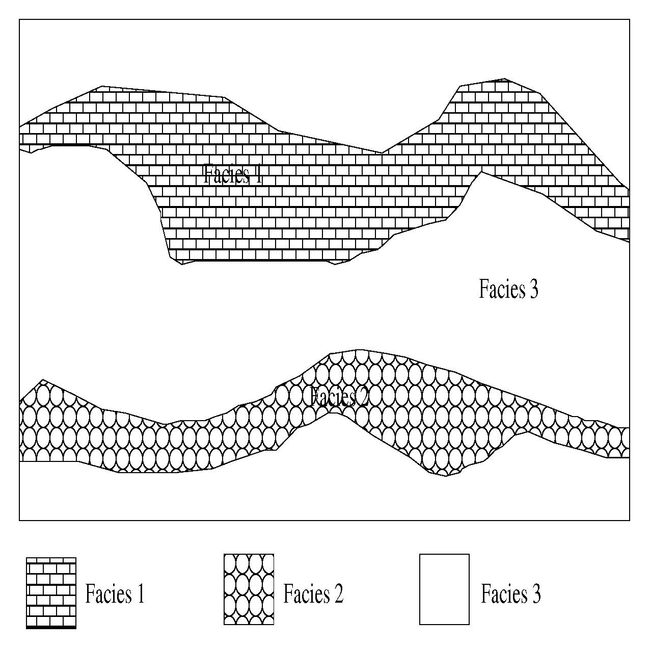
In this section, we introduce the parameterization of the permeability field. First, a heterogeneous permeability field is decomposed into several high and low permeable subregions, where each region represents a facies (see Figure 1 for illustration). This type of hierarchical representation allows us to write of the permeability field as:

$$k\left(x\right)=\sum _i{k}_i\left(x\right)I_{{\mathsf{\Omega }}_i}\left(x\right),$$

(10)

where $I_{{\mathsf{\Omega }}_i}$ is an indicator function of region ${\mathsf{\Omega }}_i$ (i.e., $I\left(x\right)=1$ if $x\in {\mathsf{\Omega }}_i$ and $I\left(x\right)=0$ otherwise). We then need to parameterize facies and interfaces. For interface, we use the level set method, while the permeability field within each facies is assumed to follow a log-Gaussian distribution with a known spatial covariance. It is to be noted that in our approach the permeability field description is defined on a finite dimension whereas the partial differential equations (PDEs) to solve the forward problem are defined on an infinite dimensional setting.

2.3.1. Parameterization of Interfaces

Suppose that any interface is a zero level set function $\phi (x,\tau )=0$. The evolution equation for an interface is given by:

$$\frac{\partial \phi }{\partial \tau }+w·\nabla \phi =0,$$

(11)

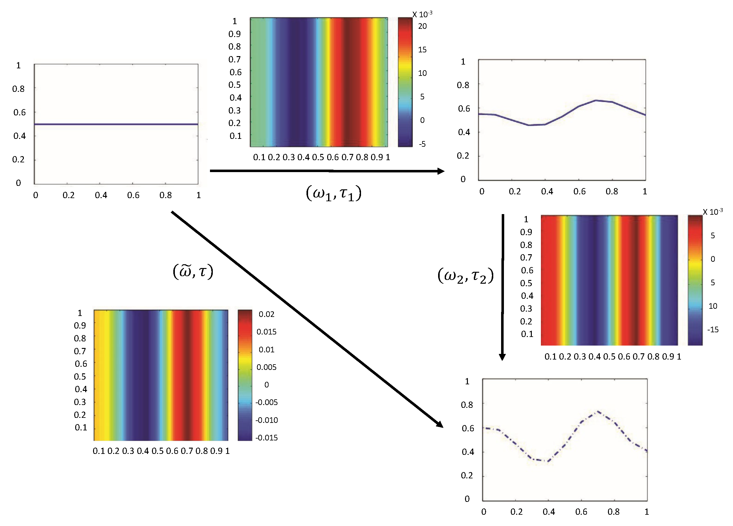
where w is a pseudo-velocity field and $\tau$ is pseudo-time. We denote ${\phi }_i$ as the $ith$ interface if there are more than one, then $\phi$ can be written as $\phi ={\phi }_i$ for different interfaces. More information on the level set method can be found in Refs. [20,22]. A key is to specify w for (11) to describe and update the boundaries of facies.

We consider a set of pseudo-velocity fields W, where $W=$ {$w|$w admits fixed streamlines, and $\left|w\right|$ is constant along streamlines on $\mathsf{\Omega }$}. In other words, we assume that the direction of the streamlines is fixed and the magnitude of the velocity along a certain streamline is the same. However the magnitudes of the velocity vary among different streamlines. In general, one can take streamline directions to be random. To keep the dimension of the parameter space small, we take streamlines to be fixed. For example, in our numerical experiment, vertical streamlines are used. We assume further that the magnitude of velocity field $w\in W$ follows the expansion,

$$\left|w\right|=\sum _i{\alpha }_i{\varphi }_i\left(z\right),{\alpha }_i\sim N(0,1),z\in {\mathsf{\Omega }}^{\prime }.$$

(12)

${\varphi }_i\left(z\right)$’s are a spatial basis for the magnitude of the velocity field and defined on the lower dimensional space of the interface, i.e., ${\varphi }_i\left(z\right)$ lives in ${\mathsf{\Omega }}^{\prime }\subset \mathsf{\Omega }$, where $dim\left({\mathsf{\Omega }}^{\prime }\right)=dim\left(\mathsf{\Omega }\right)-1$. For example, assume that $\left|w\right|$ is a second order stochastic process on ${\mathsf{\Omega }}^{\prime }$ with a given covariance structure, then ${\varphi }_i=\sqrt{{\lambda }_i}{\psi }_i$ in (12) is $L_2\left({\mathsf{\Omega }}^{\prime }\right)$ basis. In this case, $\left|w\right|$ is expressed to be a K-L expansion. More details about K-L expansion will be recalled in the next subsection.

Now, if the initial interface is $\phi (x_0,{\tau }_0)=0$ at ${\tau }_0$, the interface at ${\tau }_0+\tau$ can be written as $\phi (x_0+{\int }_{{\tau }_0}^{\tau }w\left(\tau \right)d\tau ,{\tau }_0+\tau )=0$. Any interface corresponds to a pseudo-velocity field $w\in W$ and a time $\tau$. Therefore, all interfaces of interest can be generated through the evolution Equation (11), with pair $(w,\tau )$. The following lemma proves that the set of interfaces generated through this one-step movement is well defined. Otherwise, the map between the interface set and the pseudo-velocity field W is not one-to-one.

Lemma 1.

For any $\phi (x,\tau )=0$, ∃$\tilde{w}\in W$ with Expansion (12), such that $\phi (x,\tau )=0$ can be obtained from $\phi (x_0,{\tau }_0)=0$ through evolution Equation (11).

Proof. 

For any $w_1,w_2\in W$ with $|w_1|={\sum }_i{\alpha }_{1i}{\varphi }_i\left(z\right)$ and $|w_2|={\sum }_i{\alpha }_{2i}{\varphi }_i\left(z\right)$, $z\in {\mathsf{\Omega }}^{\prime }$, the new interface formed by moving the initial $\phi (x_0,{\tau }_0)=0$ with $w_1$ and $w_2$ consecutively in time ${\tau }_1$ and ${\tau }_2$ is $\phi (x_0+{\int }_{{\tau }_0}^{{\tau }_1}{w}_{1}d\tau +{\int }_{{\tau }_1}^{{\tau }_2}{w}_{2}d\tau ,{\tau }_0+{\tau }_1+{\tau }_2)=0$.

Assuming ${\tau }_0=0$, we can choose $\tau =\sqrt{{\tau }_1^2+{\tau }_2^2}$, and let ${\tilde{\alpha }}_i=({\alpha }_{1i}{\tau }_1+{\alpha }_{2i}{\tau }_2)/\tau$, so ${\tilde{\alpha }}_i\sim N(0,1)$. For $\tilde{w}\in W$ with $|\tilde{w}|={\sum }_i{\tilde{\alpha }}_i{\varphi }_i\left(z\right)$, we have the distance of any particle in an interface moved by (11) in time interval $\tau$ as the arc length:

$$|\tilde{w}|\tau =\sum _i{\tilde{\alpha }}_i{\varphi }_i\left(z\right)\tau =\sum _i\frac{{\alpha }_{1i}{\tau }_1+{\alpha }_{2i}{\tau }_2}{\tau }\tau {\varphi }_i\left(z\right)=\sum _i{\alpha }_{1i}{\tau }_1{\varphi }_i\left(z\right)+\sum _i{\alpha }_{2i}{\tau }_2{\varphi }_i\left(z\right)=|w_1|{\tau }_1+\left|w_2\right|{\tau }_2.$$

Since $w_1$, $w_2$, and $\tilde{w}$ have the same direction at any location, this implies that ${\int }_0^{\tau }\tilde{w}d\tau ={\int }_0^{{\tau }_1}{w}_{1}d\tau +{\int }_{{\tau }_1}^{{\tau }_2}{w}_{2}d\tau$. Therefore, the new interface:

$$\phi (x,\tau )=\phi (x_0+{\int }_0^{\tau }\tilde{w}d\tau ,\tau )=\phi (x_0+{\int }_0^{{\tau }_1}{w}_{1}d\tau +{\int }_{{\tau }_1}^{{\tau }_2}{w}_{2}d\tau ,{\tau }_0+{\tau }_1+{\tau }_2)=0.$$

Namely, any interface can be obtained by moving the initial interface in a certain time period once by a $\tilde{w}\in W$, a Gaussian random field with deterministic direction.  □

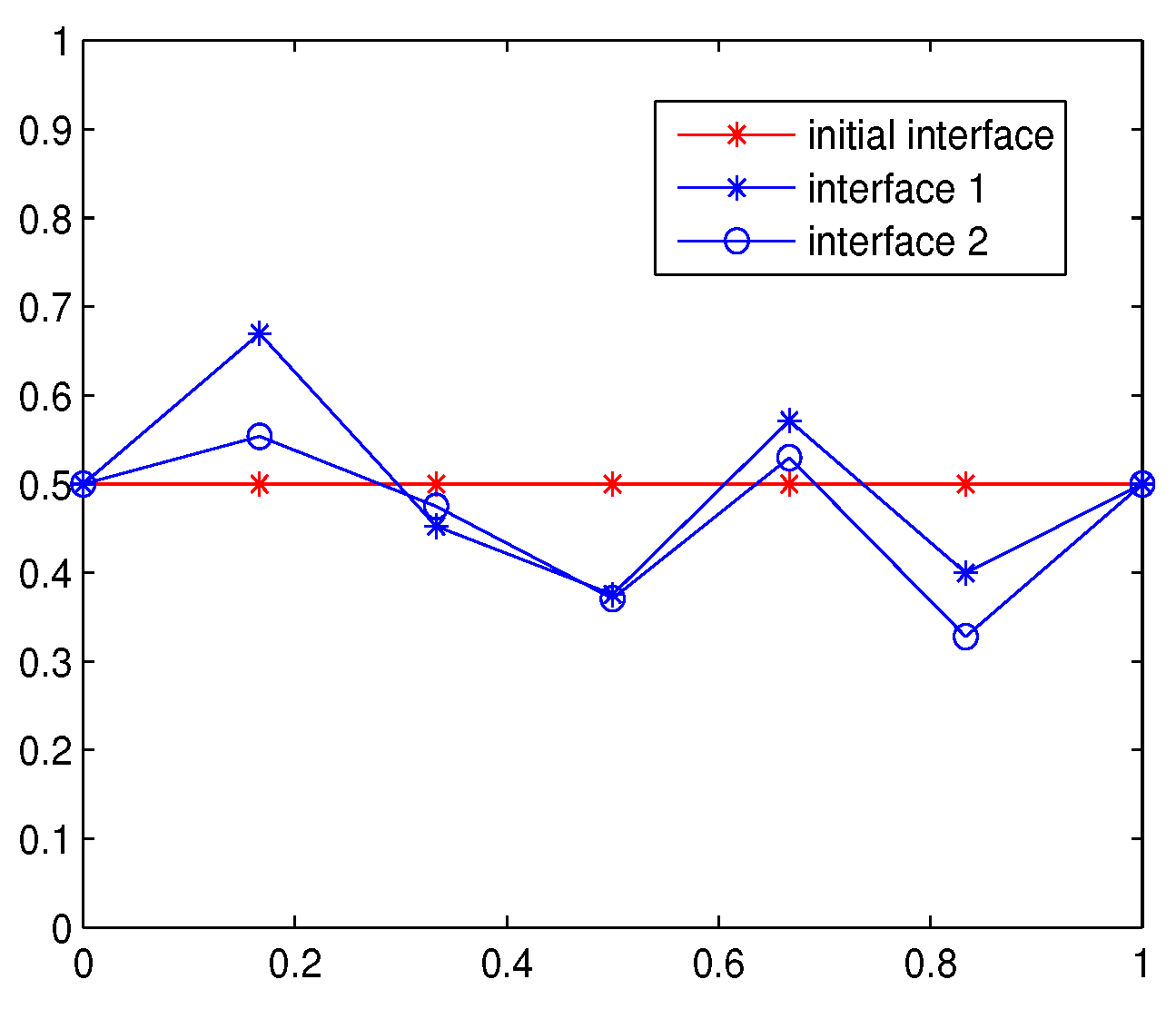
In our numerical experiments, we consider vertical streamlines in $\mathsf{\Omega }$. The pseudo-velocity is then $w=(w_x,w_y)=(0,w_y)$ and the magnitude along streamlines is assumed to be $w_y=\left|w\right|={\sum }_i{\alpha }_i{\varphi }_i\left(x\right)$, ${\alpha }_i\sim N(0,1)$, $x\in {\mathsf{\Omega }}^{\prime }$. The Lemma holds for this case, and Figure 2 illustrates the process. To get a simpler model, we also have numerical examples determining the velocity field via its values at certain discrete locations. The velocity values at these locations are updated as shown in Figure 3. In this case, the basis functions ${\varphi }_i$’s in (12) are taken to be the indicator functions for each location, and ${\alpha }_i$’s are assumed to be linear between nodes.

2.3.2. Parameterization within Facies

Now we describe the parameterization of the permeability field within the facies. The function $Y(x,\omega )=log\left[k\right(x,\omega \left)\right]$ is often considered instead of $k(x,\omega )$ as permeability is positive and distributed right skewed. Since one of the most commonly used stochastic description of spatial fields is based on a two-point correlation function, our parameterization of permeability field then starts from the correlation function of $Y(x,\omega )$, i.e., $R(x,y)=E\left[Y\right(x,\omega \left)Y\right(y,\omega \left)\right]$, where $E[·]$ refers to the expectation and x, y are points in the spatial domain. $R(x,y)$ is assumed to be known. The Karhunen–Loève expansion [29] can be used to get a parameterization of permeability field $k(x,\omega )$ or $Y(x,\omega )$ as a linear combination of a random component and spatial dependent component. The expansion is done by representing the permeability field in terms of an optimal $L^2$ basis. By truncating the expansion, we can represent the permeability matrix by fewer random parameters.

Here we briefly recall some properties of the K-L expansion. Suppose $Y(x,\omega )$ is a second order stochastic process with $E{\int }_{\mathsf{\Omega }}{Y}^2(x,\omega )dx<\infty$. For simplicity, we assume that $E\left[Y\right(x,\omega \left)\right]=0.$ Given an orthonormal basis $\left\{{\mathsf{\Phi }}_i\right\}$ in $L^2\left(\mathsf{\Omega }\right)$, we can expand $Y(x,\omega )$ as a general Fourier series:

$$Y(x,\omega )=\sum _{i=1}^{\infty }{Y}_i\left(\omega \right){\mathsf{\Phi }}_i\left(x\right),Y_i\left(\omega \right)={\int }_{\mathsf{\Omega }}Y(x,\omega ){\mathsf{\Phi }}_i\left(x\right)dx.$$

The special $L^2$ basis $\left\{{\mathsf{\Phi }}_i\right\}$ which makes the random variables $Y_i$ uncorrelated is of interest here. Namely, $E\left(Y_i{Y}_j\right)=0$ for all $i\ne j$. The basis functions $\left\{{\mathsf{\Phi }}_i\right\}$ satisfy:

$$E\left(Y_i{Y}_j\right)={\int }_{\mathsf{\Omega }}{\mathsf{\Phi }}_i\left(x\right)dx{\int }_{\mathsf{\Omega }}R(x,y){\mathsf{\Phi }}_j\left(y\right)dy=0,i\ne j.$$

Since $\left\{{\mathsf{\Phi }}_i\right\}$ is a complete basis in $L^2\left(\mathsf{\Omega }\right)$, it follows that ${\mathsf{\Phi }}_i\left(x\right)$ are eigenfunctions of $R(x,y)$,

$${\int }_{\mathsf{\Omega }}R(x,y){\mathsf{\Phi }}_i\left(y\right)dy={\lambda }_i{\mathsf{\Phi }}_i\left(x\right),i=1,2,\cdots ,$$

(13)

where ${\lambda }_i=E\left[Y_i^2\right]>0$. Furthermore, we have:

$$R(x,y)=\sum _{i=1}^{\infty }{\lambda }_i{\mathsf{\Phi }}_i\left(x\right){\mathsf{\Phi }}_i\left(y\right).$$

Denote ${\theta }_i=Y_i/\sqrt{{\lambda }_i}$, then ${\theta }_i$ satisfies $E\left({\theta }_i\right)=0$ and $E\left({\theta }_i{\theta }_j\right)={\delta }_{ij}$. It follows that:

$$Y(x,\omega )=\sum _{i=1}^{\infty }\sqrt{{\lambda }_i}{\theta }_i\left(\omega \right){\mathsf{\Phi }}_i\left(x\right),$$

(14)

where ${\mathsf{\Phi }}_i$ and ${\lambda }_i$ satisfy (13). The eigenvalues ${\lambda }_i$s can be ordered as ${\lambda }_1\ge {\lambda }_2\ge \cdots$. The $L^2$ basis functions ${\mathsf{\Phi }}_i\left(x\right)$ are deterministic and resolve the spatial dependence of the permeability field. The randomness is represented by the scalar random variables ${\theta }_i$s. The expansion (14) is called the Karhunen–Loève expansion.

In practice, a K-L expansion with finite terms rather than the infinite expansion (14) is used. Given an analytical correlation function $R(x,y)$, we can represent it on a discretized mesh. If we discretize the domain $\mathsf{\Omega }$ by an $N\times N$ rectangular mesh, we can obtain at most N pairs of eigenvalues ${\lambda }_i$ and eigenvectors ${\tilde{\mathsf{\Phi }}}_i\left(x\right)$. The ${\tilde{\mathsf{\Phi }}}_i$’s are discrete fields. To simplify the notation, we still use ${\mathsf{\Phi }}_i$ to denote ${\tilde{\mathsf{\Phi }}}_i$. In this case, the continuous K-L expansion (14) is reduced to finite terms. We get a “discretized” K-L expansion:

$$Y_N=\sum _{i=1}^N\sqrt{{\lambda }_i}{\theta }_i{\mathsf{\Phi }}_i.$$

(15)

3. Posterior Error Introduced by Truncation

In this section, we study the regularity of the posterior distribution with respect to the parameterization errors. The errors are due to using a truncated series for the velocity $\left|w\right|$ and the parameterization of permeability Y within facies. In future discussion, we use w to denote $\left|w\right|$ for simplicity.

Consider a permeability field $k(x,\omega )$ in $\mathsf{\Omega }$, see Figure 1, which has s facies ${\left\{{\mathsf{\Omega }}_i\right\}}_{i=1}^s$ and $\tilde{s}$ interfaces ${\left\{{\phi }_i\right\}}_{i=1}^{\tilde{s}}$. The number of interfaces are assumed to be known and the interfaces are continuous. Each facies is described by a covariance matrix $R_i(x,y)$ as in Section 2.3.2. Then, the permeability field $k(x,\omega )$ is a function given by:

$$k(x,\omega )=\sum _{i=1}^s{k}_i(x,\omega )I_{{\mathsf{\Omega }}_i}\left(x\right),$$

where $I_{{\mathsf{\Omega }}_i}$ is an indicator function on ${\mathsf{\Omega }}_i$. Through K-L expansion, the permeability of each facies ${\mathsf{\Omega }}_i$ is $k_i(x,\omega )=exp\left\{Y_i(x,\omega )\right\}=exp\{{\sum }_{j=1}^{\infty }\sqrt{{\lambda }_{ij}}{\theta }_{ij}{\psi }_{ij}\left(x\right)\}$, and each interface is formed by moving the initial interface ${\phi }_i(x,t_0)=0$ by a velocity field with deterministic direction $w_i={\sum }_{j=1}^{\infty }{\alpha }_{ij}{\varphi }_{ij}\left(z\right)$ as in Section 2.3.1. Then, the permeability field $k(x,\omega )$ can be written as:

$$k(x,\theta ,\alpha )=\sum _{i=1}^{s}exp\left(Y_i\right)I_{{\mathsf{\Omega }}_i\left(\alpha \right)}\left(x\right).$$

Considering the finite discretized case allows us to write $Y_i$ and $w_i$ in each ${\mathsf{\Omega }}_i$ as $Y_{N_i}={\sum }_{j=1}^{N_i}\sqrt{{\lambda }_{ij}^{\left(\theta \right)}}$${\theta }_{ij}{\psi }_{ij}\left(x\right)$, $i=1,\cdots ,s$, $x\in \mathsf{\Omega }$ and $w_{{\tilde{N}}_i}={\sum }_{j=1}^{{\tilde{N}}_i}\sqrt{{\lambda }_{ij}^{\left(\alpha \right)}}{\alpha }_{ij}{\varphi }_{ij}\left(z\right)$, $i=1,\cdots ,\tilde{s}$, $z\in {\mathsf{\Omega }}^{\prime }$ with $dim\mathsf{\Omega }=dim{\mathsf{\Omega }}^{\prime }+1$. Note that ${\lambda }_{ij}^{\left(\theta \right)}$ and ${\lambda }_{ij}^{\left(\alpha \right)}$ usually decrease to 0 fast, the truncated K-L expansions, i.e., $Y_{M_i}={\sum }_{i=1}^{M_i}\sqrt{{\lambda }_{ij}^{\left(\theta \right)}}{\theta }_{ij}{\psi }_{ij}$ and $w_{\widetilde{M_i}}={\sum }_{j=1}^{\widetilde{M_i}}\sqrt{{\lambda }_{ij}^{\left(\alpha \right)}}{\alpha }_{ij}{\varphi }_{ij}$ can be used to reduce the dimension of the parameter space, which in turn would save CPU time while sampling from the posterior distribution. We denote $\theta =({\theta }_{11},\cdots ,{\theta }_{1N_1},\cdots ,{\theta }_{s1},\cdots ,{\theta }_{s{N}_s})$ and $\alpha =({\alpha }_{11},\cdots ,{\alpha }_{1{\tilde{N}}_1},\cdots ,{\alpha }_{(s-1)1},\cdots ,{\alpha }_{\tilde{s}{\tilde{N}}_{\tilde{s}}})$, where $({\theta }_{i1},\cdots ,{\theta }_{i{N}_i})$ describe the permeability field $k(\theta ,\alpha )$ within the $ith$ facies and $({\alpha }_{j1},\cdots ,{\alpha }_{j{\tilde{N}}_j})$ describe the $jth$ interface. ${\theta }_M$ and ${\alpha }_{\tilde{M}}$ are truncations of $\theta$ and $\alpha$, respectively. Then, the corresponding representations of the permeability field in full and truncated case are given by:

$$\begin{array}{ccc}\hfill k(\theta ,\alpha )& =& \sum _{i=1}^{s}exp\left(\sum _{j=1}^{N_i}\sqrt{{\lambda }_{ij}^{\left(\theta \right)}}{\theta }_{ij}{\psi }_{ij}\right)I_{\left\{{\mathsf{\Omega }}_i({\alpha }_{i1},\cdots ,{\alpha }_{i{\tilde{N}}_i})\right\}},\hfill \\ \hfill k({\theta }_M,{\alpha }_{\tilde{M}})& =& \sum _{i=1}^{s}exp\left(\sum _{j=1}^{M_i}\sqrt{{\lambda }_{ij}^{\left(\theta \right)}}{\theta }_{ij}{\psi }_{ij}\right)I_{\left\{{\mathsf{\Omega }}_i({\alpha }_{i1},\cdots ,{\alpha }_{i{\tilde{M}}_i})\right\}}.\hfill \end{array}$$

Correspondingly, the two posterior distributions of the permeability field in the Bayesian framework are given by:

$$\begin{array}{ccc}\hfill \pi (\theta ,\alpha )& \propto & G(\theta ,\alpha )\prod _{i=1}^s{\pi }_0({\theta }_{i1},\cdots ,{\theta }_{i{N}_i})\prod _{j=1}^{\tilde{s}}{\pi }_0({\alpha }_{j1},\cdots ,{\alpha }_{j{\tilde{N}}_j}),\hfill \\ \hfill \tilde{\pi }(\theta ,\alpha )& \propto & \tilde{G}({\theta }_M,{\alpha }_{\tilde{M}})\prod _{i=1}^s{\pi }_0({\theta }_{i1},\cdots ,{\theta }_{i{N}_i})\prod _{j=1}^{\tilde{s}}{\pi }_0({\alpha }_{j1},\cdots ,{\alpha }_{j{\tilde{N}}_j}),\hfill \end{array}$$

where $G(\theta ,\alpha )=exp(-{\int }_0^T|F_{obs}-F(k{(\theta ,\alpha );t)|}^{2}dt/{\sigma }_f^2)$, $\tilde{G}({\theta }_M,{\alpha }_{\tilde{M}})=exp(-{\int }_0^T|F_{obs}-F(k({\theta }_M,$${\alpha }_{\tilde{M}}){;t)|}^{2}dt/{\sigma }_f^2)$, and $F_{obs}$ is the observed fractional flow data. The priors ${\pi }_0(\theta ,\alpha )$ is assumed to be the product Gaussian measure.

It is clear that this truncation process affects the posterior inference. Our goal here is to estimate the error introduced by this truncation, which can also provide a guidance to choose $M_i$ and ${\tilde{M}}_j$ for specific requirements. A case with single facies is considered first before we state the main theorem involving multiple facies.

Theorem 1.

Assume that the assumptions in Appendix A hold, and suppose the log-permeability field $Y={\sum }_{i=1}^N\sqrt{{\lambda }_i}{\theta }_i{\psi }_i$ is a stationary spatial process on a bounded region, with the truncation $\tilde{Y}={\sum }_{i=1}^M\sqrt{{\lambda }_i}{\theta }_i{\psi }_i$, and $f\left(\theta \right)$ is a square integrable with respect to Gaussian measure, i.e., ${\int \left|f\left(\theta \right)\right|}^2{\pi }_0\left(\theta \right)d\theta <\infty$, then:

$$\begin{array}{c}\hfill |E_{\pi \left(\theta \right)}\left[f\left(\theta \right)\right]-E_{\tilde{\pi }\left(\theta \right)}\left[f\left(\theta \right)\right]|\le C{\left\{\sum _{i=M+1}^N{\lambda }_i\right\}}^{\frac{1}{2}},\end{array}$$

(16)

where C is independent of dimension N.

To prove this result, the main estimation of the fractional flow error $|F(k_1;t)-F(k_2,t)|$ is obtained from estimation of the governing PDE system (1)–(3). Details are provided in Appendix A. For a general case, when the permeability field has more than one facies, we can state the main theorem.

Theorem 2.

Assume that the assumptions in Appendix A hold, and suppose the discretized K-L expansion of the log permeability field and the random velocity field are given by $Y_{N_i}={\sum }_{j=1}^{N_i}\sqrt{{\lambda }_{ij}^{\left(\theta \right)}}{\theta }_{ij}{\psi }_i\left(x\right)$ and $w_{{\tilde{N}}_i}={\sum }_{j=1}^{{\tilde{N}}_i}\sqrt{{\lambda }_{ij}^{\left(\alpha \right)}}{\alpha }_{ij}{\varphi }_{ij}\left(z\right)$, where all $Y_{N_i}$ and $w_{{\tilde{N}}_i}$ are stationary spatial processes on a bounded region, and the truncated expansions are $Y_{M_i}={\sum }_{j=1}^{M_i}\sqrt{{\lambda }_{ij}^{\left(\theta \right)}}{\theta }_{ij}{\psi }_{ij}$ and $w_{\widetilde{M_i}}={\sum }_{j=1}^{\widetilde{M_i}}\sqrt{{\lambda }_{ij}^{\left(\alpha \right)}}{\alpha }_{ij}{\varphi }_{ij}$ respectively. Assume that $f(\theta ,\alpha )$ is a square integrable function with respect to Gaussian measure, i.e., ${\int \left|f(\theta ,\alpha )\right|}^2{\pi }_0(\theta ,\alpha )d\theta d\alpha <\infty$, then:

$$\begin{array}{c}\hfill \left|E_{\pi (\theta ,\alpha )}\left[f(\theta ,\alpha )\right]-E_{\tilde{\pi }(\theta ,\alpha )}\left[f(\theta ,\alpha )\right]\right|\le C_1\underset{1\le i\le s}{max}{\left\{\sum _{j=M_i+1}^{N_i}{\lambda }_{ij}^{\left(\theta \right)}\right\}}^{\frac{1}{2}}+C_2\underset{1\le i\le \tilde{s}}{max}{\left\{\sum _{j={\tilde{M}}_i+1}^{{\tilde{N}}_i}{\lambda }_{ij}^{\left(\alpha \right)}\right\}}^{\frac{1}{2}},\end{array}$$

(17)

where $C_1$ and $C_2$ are independent of dimension $N_i$ and ${\tilde{N}}_i$.

Proof. 

Note that:

$$\left|E_{\pi (\theta ,\alpha )}\left[f(\theta ,\alpha )\right]-E_{\tilde{\pi }(\theta ,\alpha )}\left[f(\theta ,\alpha )\right]\right|\le C(E_1+E_2),$$

where:

$$\begin{array}{ccc}\hfill E_1& =& \int \left|f(\theta ,\alpha )\right| · |\tilde{G}(\theta ,{\alpha }_{\tilde{M}})-\tilde{G}({\theta }_M,{\alpha }_{\tilde{M}})|{\pi }_0(\theta ,\alpha )d(\theta ,\alpha ),\hfill \\ \hfill E_2& =& \int \left|f(\theta ,\alpha )\right| · |G(\theta ,\alpha )-\tilde{G}(\theta ,{\alpha }_{\tilde{M}})|{\pi }_0(\theta ,\alpha )d(\theta ,\alpha ).\hfill \end{array}$$

It is clear that Lemma A3 can be generalized to the multi-facies case to get $|\tilde{G}(\theta ,{\alpha }_{\tilde{M}})-\tilde{G}({\theta }_M,{\alpha }_{\tilde{M}})|\le \frac{C}{{\sigma }_f^2}{\sum }_{i=1}^s\parallel k({\theta }_{i1},\cdots ,{\theta }_{i{N}_i})-k({\theta }_{i1},\cdots ,$${\theta }_{i{M}_i}{)\parallel }_{L_2\left({\mathsf{\Omega }}_i\left({\alpha }_{\tilde{M}}\right)\right)}$. Then,

$$\begin{array}{ccc}\hfill E_1& \le & \frac{C}{{\sigma }_f^2}\int |f(\theta ,\alpha )|\sum _{i=1}^s{\parallel k({\theta }_{i1},\cdots ,{\theta }_{i{N}_i})-k({\theta }_{i1},\cdots ,{\theta }_{i{M}_i})\parallel }_{L_2\left({\mathsf{\Omega }}_i\left({\alpha }_{\tilde{M}}\right)\right)}{\pi }_0(\theta ,\alpha )d(\theta ,\alpha )\hfill \\ & \le & \frac{C}{{\sigma }_f^2}\int \sum _{i=1}^s\int |f(\theta ,\alpha )|·||k({\theta }_{i1},\cdots ,{\theta }_{i{N}_i})-k({\theta }_{i1},\cdots ,{\theta }_{i{M}_i}){\parallel }_{L_2\left({\mathsf{\Omega }}_i\left({\alpha }_{\tilde{M}}\right)\right)}{\pi }_0\left(\theta \right)d\theta {\pi }_0\left(\alpha \right)d\alpha \hfill \\ & \le & \frac{C}{{\sigma }_f^2}\int \sum _{i=1}^s{\{\int |f(\theta ,\alpha )|}^2{\pi }_0{\left(\theta \right)d\theta \}}^{\frac{1}{2}}\hfill \\ & & ·\{\int \parallel k({\theta }_{i1},\cdots ,{\theta }_{i{N}_i})-k({\theta }_{i1},\cdots ,{\theta }_{i{M}_i}){{\parallel }_{L_2\left({\mathsf{\Omega }}_i\left({\alpha }_{\tilde{M}}\right)\right)}^2{\pi }_0\left(\theta \right)d\theta \}}^{\frac{1}{2}}{\pi }_0\left(\alpha \right)d\alpha \hfill \\ & \le & C\int \sum _{i=1}^s{\left\{\sum _{j=M_i+1}^{N_i}{\lambda }_{ij}^{\left(\theta \right)}\right\}}^{\frac{1}{2}}{\pi }_0\left(\alpha \right)d\alpha \le C\underset{1\le i\le s}{max}{\left\{\sum _{j=M_i+1}^{N_i}{\lambda }_{ij}^{\left(\theta \right)}\right\}}^{\frac{1}{2}},\hfill \end{array}$$

by Theorem 1. To estimate $E_2$, the corresponding error estimation for permeability fields is also needed, i.e.,

$$\begin{array}{ccc}& & \parallel k(\theta ,\alpha )-k(\theta ,{\alpha }_{{}_{\tilde{M}}}){\parallel }_{L_2\left(\mathsf{\Omega }\right)}^2\hfill \\ & =& \underset{\mathsf{\Omega }}{\int }{\left|\sum _{i=1}^s{k}_i{I}_{{\mathsf{\Omega }}_i\left(\alpha \right)}-\sum _{i=1}^s{k}_i{I}_{{\mathsf{\Omega }}_i\left({\alpha }_{{}_{\tilde{M}}}\right)}\right|}^{2}dx\le C\sum _{i=1}^{\tilde{s}}\underset{{\mathsf{\Omega }}^{\prime }}{\int }{k}_i^2{|w_{{\tilde{N}}_i}-w_{\widetilde{M_i}}|}^{2}dz\hfill \\ & \le & C\sum _{i=1}^{\tilde{s}}\underset{{\mathsf{\Omega }}^{\prime }}{\int }{k}_i^2{\left|\sum _{j={\tilde{M}}_i+1}^{{\tilde{N}}_i}\sqrt{{\lambda }_{ij}^{\left(\alpha \right)}}{\alpha }_{ij}{\varphi }_{ij}\right|}^{2}dz\le C\sum _{i=1}^{\tilde{s}}\underset{{\mathsf{\Omega }}^{\prime }}{\int }{k}_i^{2}exp\left(2\sum _{j={\tilde{M}}_i+1}^{{\tilde{N}}_i}\sqrt{{\lambda }_{ij}^{\left(\alpha \right)}}{\alpha }_{ij}{\varphi }_{ij}\right)dz.\hfill \end{array}$$

Then we can estimate $E_2$ as:

$$\begin{array}{ccc}\hfill E_2& \le & \frac{C}{{\sigma }_f^2}{\{\int |f(\theta ,\alpha )|}^2{\pi }_0{(\theta ,\alpha )d(\theta ,\alpha )\}}^{\frac{1}{2}}·\{\int ||k(\theta ,\alpha )-k(\theta ,{\alpha }_{{}_{\tilde{M}}}){||}_{L_2\left(\mathsf{\Omega }\right)}^2{\pi }_0(\theta ,\alpha )d(\theta ,\alpha ){\}}^{\frac{1}{2}}\hfill \\ & \le & \frac{C}{{\sigma }_f^2}{\{\int \sum _{i=1}^{\tilde{s}}\underset{{\mathsf{\Omega }}^{\prime }}{\int }{k}_i^{2}exp\left(2\sum _{j={\tilde{M}}_i+1}^{{\tilde{N}}_i}\sqrt{{\lambda }_{ij}^{\left(\alpha \right)}}{\alpha }_{ij}{\varphi }_{ij}\right)dz{\pi }_0(\theta ,\alpha )d(\theta ,\alpha )\}}^{\frac{1}{2}}\hfill \\ & \le & \frac{C}{{\sigma }_f^2}{\{\underset{{\mathsf{\Omega }}^{\prime }}{\int }[\sum _{i=1}^{\tilde{s}}\int k_i^2{\pi }_0\left({\theta }_i\right)d{\theta }_i\int exp\left(2\sum _{j={\tilde{M}}_i+1}^{{\tilde{N}}_i}\sqrt{{\lambda }_{ij}^{\left(\alpha \right)}}{\alpha }_{ij}{\varphi }_{ij}\right){\pi }_0\left({\alpha }_i\right)d{\alpha }_i]dz\}}^{\frac{1}{2}}\hfill \\ & \le & \frac{C}{{\sigma }_f^2}{\{\sum _{i=1}^{\tilde{s}}\underset{{\mathsf{\Omega }}^{\prime }}{\int }exp\left(2\sum _{j=1}^N{\lambda }_{ij}^{\left(\theta \right)}{\psi }_{ij}^2\right)exp\left(2\sum _{j={\tilde{M}}_i+1}^{{\tilde{N}}_i}{\lambda }_{ij}^{\left(\alpha \right)}{\varphi }_{ij}^2\right)dz\}}^{\frac{1}{2}}\hfill \\ & \le & C\underset{1\le i\le \tilde{s}}{max}{\left\{\sum _{j={\tilde{M}}_i+1}^{{\tilde{N}}_i}{\lambda }_{ij}^{\left(\alpha \right)}\right\}}^{\frac{1}{2}}.\hfill \end{array}$$

Since all $Y_{N_i}$ and $w_{{\tilde{N}}_i}$ are stationary spatial processes on a bounded region, i.e., spatial processes where the covariance function depends only on the distance not on the spatial location, the eigenfunctions $\left\{{\psi }_{ij}\right\}$ and $\left\{{\varphi }_{ij}\right\}$ are uniform $L_{\infty }\left(\mathsf{\Omega }\right)$ bounded (see [30]). Thus:

$$\begin{array}{c}\hfill \left|E_{\pi (\theta ,\alpha )}\left[f(\theta ,\alpha )\right]-E_{\tilde{\pi }(\theta ,\alpha )}\left[f(\theta ,\alpha )\right]\right|\le C_1\underset{1\le i\le s}{max}{\left\{\sum _{j=M_i+1}^{N_i}{\lambda }_{ij}^{\left(\theta \right)}\right\}}^{\frac{1}{2}}+C_2\underset{1\le i\le \tilde{s}}{max}{\left\{\sum _{j={\tilde{M}}_i+1}^{{\tilde{N}}_i}{\lambda }_{ij}^{\left(\alpha \right)}\right\}}^{\frac{1}{2}}.\end{array}$$

Please note that as $C_1$ and $C_2$ are independent of $N_i$ and ${\tilde{N}}_i$, when $M_i\to N_i$ and ${\tilde{M}}_i\to {\tilde{N}}_i$, we have $\left|E_{\pi (\theta ,\alpha )}\left(f(\theta ,\alpha )\right)-E_{\tilde{\pi }(\theta ,\alpha )}\left(f(\theta ,\alpha )\right)\right|\to 0$.  □

The theorem here shows the possibility to lower the dimension of the inverse problem by truncating K-L expansions. Without truncation, the dimension of K-L expansions of the permeability field and pseudo-velocity field, which is decided by the dimension of discretization, can be very large. A large dimension requires more iterations for the MCMC method to converge and therefore makes the computation expensive, if not infeasible. The theorem provides a bound to the error of the two posteriors and confirms the validity of the truncation of the parameter space without introducing unbounded errors. To choose $M_i$ and ${\tilde{M}}_i$ a priori, estimations of $C_1$ and $C_2$ are needed. The constants $C_1$ and $C_2$ are independent of $N_i$ and ${\tilde{N}}_i$, but they are dependent on the square integrable function f and other factors. It is also possible to estimate C numerically.

4. MCMC Sampling from the Truncated Posterior

In this section, we introduce the sampling scheme used in the numerical examples in Section 5.2. To see the advantages of this scheme, we first state the standard Metropolis–Hastings algorithm and then point out the motivation of using the scheme.

For channelized permeability field, the standard Metropolis–Hastings (M-H) algorithm can be formed in the following way to sample from the truncated posterior distribution $P\left(k\right|F_{obs})$.

Algorithm (M-H MCMC [31]): Suppose at the $nth$ step, we have permeability field $k_n({\alpha }_n,{\theta }_n)$.

Step 1. Generate $\alpha$ from a distribution $q_{\alpha }\left(\alpha \right|{\alpha }_n)$ and $\theta$ from a distribution $q_{\theta }\left(\theta \right|{\theta }_n)$. Then the entire permeability field is proposed using (10).

Step 2. Accept k as a sample with probability:

$$\begin{array}{ccc}\hfill \gamma (k_n,k)& =& min\left\{1,\frac{\pi \left(k\right)q\left(k_n\right|k)}{\pi \left(k_n\right)q\left(k\right|k_n)}\right\}\hfill \\ & =& min\left\{1,\frac{P\left(F_{obs}\right|k)}{P\left(F_{obs}\right|k_n)}·\frac{P\left(\alpha \right)P\left(\theta \right)}{P\left({\alpha }_n\right)P\left({\theta }_n\right)}·\frac{q_{\alpha }\left({\alpha }_n\right|\alpha )q_{\theta }\left({\theta }_n\right|\theta )}{q_{\alpha }\left(\alpha \right|{\alpha }_n)q_{\theta }\left(\theta \right|{\theta }_n)}\right\},\hfill \end{array}$$

(18)

i.e., take $k_{n+1}=k$ with probability $\gamma (k_n,k)$, and $k_{n+1}=k_n$ with probability $1-\gamma (k_n,k)$.  □

Starting with an initial permeability sample $k_0$, the MCMC algorithm generates a Markov chain $\left\{k_n\right\}$ with the transition kernel as:

$$\begin{array}{ccc}\hfill K_r(k_n,k)& =& \gamma (k_n,k)q\left(k\right|k_n)+\left(1-\int \gamma (k_n,k)q\left(k\right|k_n)dk\right){\delta }_{k_n}\left(k\right)\hfill \\ & =& \gamma (k_n,k)q_{\alpha }\left(\alpha \right|{\alpha }_n)q_{\theta }\left(\theta \right|{\theta }_n)+\left(1-\int \gamma (k_n,k)q_{\alpha }\left(\alpha \right|{\alpha }_n)q_{\theta }\left(\theta \right|{\theta }_n)d\alpha d\theta \right){\delta }_{{\alpha }_n}\left(\alpha \right){\delta }_{{\theta }_n}\left(\theta \right).\hfill \end{array}$$

The target distribution $\pi \left(k\right)$ is the stationary distribution of the Markov chain $\left\{k_n\right\}$, so $k_n$ represents the sample generated from $\pi \left(k\right)$ after the chain converges and reaches a steady state.

The main disadvantage of the MCMC algorithm is the high computational cost in solving the coupled nonlinear PDE system (1)–(3) on the fine-grid in order to compute $F_k$ in the target distribution $\pi \left(k\right)$. Typically, the MCMC method in our simulations converges to the steady-state after thousands of iterations, and the acceptance rate is also quite low. A large amount of CPU time is spent on simulating the rejected samples. The MCMC method can be improved by adapting the proposal distribution $q\left(k\right|k_n)$ to the target distribution using a coarse-scale model. The process essentially modifies the proposal distribution $q\left(k\right|k_n)$ by incorporating the coarse-scale information. The algorithm for a general two-stage MCMC method with upscaling was introduced in [32].

Let $F_k^{*}$ be the fractional flow computed by solving the coarse-scale model of (1)–(3) for the given k. This is done with mixed MsFEM [28]. Mixed MsFEM is used to solve pressure, and saturation is solved on a coarse grid. The fine-scale target distribution $\pi \left(k\right)$ is approximated on the coarse-scale by ${\pi }^{*}\left(k\right)$. Here, we have:

$$\pi \left(k\right)\propto exp\left(-\frac{\parallel F_{obs}-F_k{\parallel }^2}{{\sigma }_f^2}\right)P\left(k\right),$$

$${\pi }^{*}\left(k\right)\propto exp\left(-\frac{\left(\mathfrak{G}\right(\parallel F_{obs}-F_k^{*}{\parallel \left)\right)}^2}{{\sigma }_c^2}\right)P\left(k\right),$$

where the function $\mathfrak{G}$ is estimated based on offline computations using independent samples from the prior. Using the coarse-scale distribution ${\pi }^{*}\left(k\right)$ as a filter, the two-stage MCMC can be described as follows.

Algorithm (Two-stage MCMC [32]): Suppose at the $nth$ step, we have ${\alpha }_n$, ${\theta }_n$, and permeability field $k_n$.

Coarse stage:

Step 1. At $k_n$, generate a trial proposal $\tilde{k}$ from distribution $q_{\alpha }\left(\alpha \right|{\alpha }_n)$ and $q_{\theta }\left(\theta \right|{\theta }_n)$. The fractional flow $F_k^{*}$ is computed by solving the coarse-scale model.

Step 2. Take the proposal as:

$$k=\left\{\begin{array}{cc}\tilde{k}\hfill & \mathrm{with}\mathrm{probability}{\gamma }_p(k_n,\tilde{k}),\hfill \\ k_n\hfill & \mathrm{with}\mathrm{probability}1-{\gamma }_p(k_n,\tilde{k}).\hfill \end{array}\right.$$

The acceptance probability is given by:

$${\gamma }_p(k_n,\tilde{k})=min\left\{1,\frac{P^{*}\left(F_{obs}\right|\tilde{k})}{P^{*}\left(F_{obs}\right|k_n)}·\frac{P\left(\alpha \right)P\left(\theta \right)}{P\left({\alpha }_n\right)P\left({\theta }_n\right)}·\frac{q_{\alpha }\left({\alpha }_n\right|\alpha )q_{\theta }\left({\theta }_n\right|\theta )}{q_{\alpha }\left(\alpha \right|{\alpha }_n)q_{\theta }\left(\theta \right|{\theta }_n)}\right\}.$$

(19)

Therefore, the final proposal k is generated from the effective instrumental distribution:

$$Q(k|k_n)={\gamma }_p(k_n,k)q(k|k_n)+(1-\int {\gamma }_p(k_n,k)q\left(k\right|k_n)dk){\delta }_{k_n}\left(k\right).$$

If $k=\tilde{k}$, go to the Step 3. Otherwise, i.e., $k=k_n$, return to Step 1.

Fine stage:

Step 3. Accept k as a sample with probability:

$${\gamma }_f(k_n,k)=min\left(1,\frac{Q\left(k_n\right|k)\pi \left(k\right)}{Q\left(k\right|k_n)\pi \left(k_n\right)}\right),$$

(20)

i.e., $k_{n+1}=k$ with probability ${\gamma }_f(k_n,k)$, and $k_{n+1}=k_n$ with probability $1-{\gamma }_f(k_n,k)$.  □

Using the argument as in [32], the acceptance probability (20) can be simplified as:

$${\gamma }_f(k_n,k)=min\left(1,\frac{\pi \left(k\right){\pi }^{*}\left(k_n\right)}{\pi \left(k_n\right){\pi }^{*}\left(k\right)}\right).$$

In our numerical example, we use a random walk to generate proposals, i.e., at the $nth$ step, we propose $\alpha ={\alpha }_n+h_{\alpha }{u}_{\alpha }$, where $u_{\alpha }$ is generated from a $N(0,I)$ distribution. Similarly, we propose $\theta ={\theta }_n+h_{\theta }{u}_{\theta }$, where $u_{\theta }$ is also generated from a $N(0,I)$ distribution. Here $h_{\alpha }$ and $h_{\theta }$ represent the step size of the jump in each iteration of the Metropolis–Hastings algorithm. The values of $h_{\alpha }$ and $h_{\theta }$ control the convergence of the MCMC algorithm. The prior distribution of $\alpha$ can be taken to be $N({\alpha }_o,{\sigma }_{\alpha }^{2}I)$. Similarly, the prior distribution of $\theta$ can be taken to be $N({\theta }_o,{\sigma }_{\theta }^{2}I)$. Then, our acceptance probability (18) is given by:

$$\gamma (k_n,k)=min\left\{1,\frac{exp\left(\frac{-\parallel F_{obs}-F_k{\parallel }^2}{2{\sigma }_f^2}\right)}{exp\left(\frac{-\parallel F_{obs}-F_{k_n}{\parallel }^2}{2{\sigma }_f^2}\right)}\frac{exp\left(\frac{-\parallel \theta -{\theta }_o{\parallel }^2}{2{\sigma }_{\theta }^2}+\frac{-\parallel \alpha -{\alpha }_o{\parallel }^2}{2{\sigma }_{\alpha }^2}\right)}{exp\left(\frac{-\parallel {\theta }_n-{\theta }_o{\parallel }^2}{2{\sigma }_{\theta }^2}+\frac{-\parallel {\alpha }_n-{\alpha }_o{\parallel }^2}{2{\sigma }_{\alpha }^2}\right)}\right\}.$$

(21)

The acceptance probability (19) in the two-stage MCMC algorithm is similar.

We also use a simple relation for modeling coarse- and fine-scale errors. In particular, $\mathfrak{G}$ is taken to be a linear function with the condition $\mathfrak{G}\left(0\right)=0$. Then, ${\pi }^{*}\left(k\right)$ becomes:

$${\pi }^{*}\left(k\right)\propto exp\left(-\frac{\parallel F_{obs}-F_k^{*}{\parallel }^2}{{\sigma }_c^2}\right)P\left(k\right),$$

i.e., on the coarse-scale $F_{obs}|k$ is assumed to follow $N(F_k^{*},{\sigma }_c^{2}I)$ distribution,

$$P^{*}\left(F_{obs}\right|k)\propto exp\left(-\frac{\parallel F_{obs}-F_k^{*}{\parallel }^2}{{\sigma }_c^2}\right),$$

where ${\sigma }_c$ is the precision associated with the coarse-scale model. The parameter ${\sigma }_c$ plays an important role in improving the acceptance rate of the preconditioned MCMC method. The optimal value of ${\sigma }_c$ depends on the correlation between $\parallel F-F_k\parallel$ and $\parallel F-F_k^{*}\parallel$, which can be estimated by offline computations.

Assuming that on the fine-scale $F_{obs}|k$ follows a $N(F_k,{\sigma }_f^{2}I)$ distribution, i.e.,

$$P\left(F_{obs}\right|k)\propto exp\left(-\frac{\parallel F_{obs}-F_k{\parallel }^2}{{\sigma }_f^2}\right),$$

the acceptance probability (21) becomes:

$${\gamma }_f(k_n,k)=min\left(1,\frac{exp\left(-\frac{\parallel F_{obs}-F_k{\parallel }^2}{{\sigma }_f^2}\right)exp\left(-\frac{\parallel F_{obs}-F_{k_n}^{*}{\parallel }^2}{{\sigma }_c^2}\right)}{exp\left(-\frac{\parallel F_{obs}-F_{k_n}{\parallel }^2}{{\sigma }_f^2}\right)exp\left(-\frac{\parallel F_{obs}-F_k^{*}{\parallel }^2}{{\sigma }_c^2}\right)}\right).$$

(22)

5. Numerical Results

5.1. Convergence Estimation

The numerical results are presented here to validate the results from Theorems 1 and 2 on truncation error estimation. We consider the water-cut function (7) as our $f\left(\right)$ in the theorems, because it is an important property for reservoirs. First, the tests are completed for single facies permeability field, and then channelized cases are considered.

5.1.1. Single Facies

In the first simulation example, a permeability field without any channelized structure is considered. To describe the permeability field, a two-point correlation function is defined as:

$$R(x,y)={\sigma }^{2}exp\left(-\frac{|x_1-y_1{|}^2}{2l_1^2}-\frac{|x_2-y_2{|}^2}{2l_2^2}\right).$$

(23)

K-L expansion is then used to describe the permeability field. $f\left(\theta \right)$ (the quantity of interest) is taken to be water-cut function F. One injector at $(0,0.5)$ and one producer at $(1,0.5)$ are considered when we run the forward model in the reference permeability field to get the fractional flow as discussed in Section 2.1. The numerical results for the error estimation are shown in

Table 1. Posterior errors $|E_{\pi }F-E_{\tilde{\pi }}F|$ when the K-L expansion is truncated to M terms. Here $l_1=0.1$, $l_2=0.4$, ${\sigma }^2=2$, and ${\sigma }_f^2=0.001$.

M	${\left({\sum }_{\mathit{i}=\mathit{M}+1}^{\mathit{N}}{\mathit{\lambda }}_{\mathit{i}}^{\left(\mathit{\theta }\right)}\right)}^{\frac{1}{2}}$	$|{\mathit{E}}_{\mathit{\pi }}\mathit{F}-{\mathit{E}}_{\tilde{\mathit{\pi }}}\mathit{F}|$
5	1.111681	0.081809
10	0.750662	0.106264
15	0.517555	0.063635
20	0.337901	0.030207
25	0.189272	0.017931
30	0.071924	0.011225

and

Table 2. Posterior errors $|E_{\pi }F-E_{\tilde{\pi }}F|$ when the K-L expansion is truncated to M terms. Here $l_1=0.2$, $l_2=0.2$, ${\sigma }^2=2$, and ${\sigma }_f^2=0.005$.

M	${\left({\sum }_{\mathit{i}=\mathit{M}+1}^{\mathit{N}}{\mathit{\lambda }}_{\mathit{i}}^{\left(\mathit{\theta }\right)}\right)}^{\frac{1}{2}}$	$|{\mathit{E}}_{\mathit{\pi }}\mathit{F}-{\mathit{E}}_{\tilde{\mathit{\pi }}}\mathit{F}|$
5	1.176697	0.308118
10	0.820661	0.191601
15	0.566938	0.119590
20	0.378454	0.059173
25	0.248267	0.033023
30	0.123347	0.014965

.

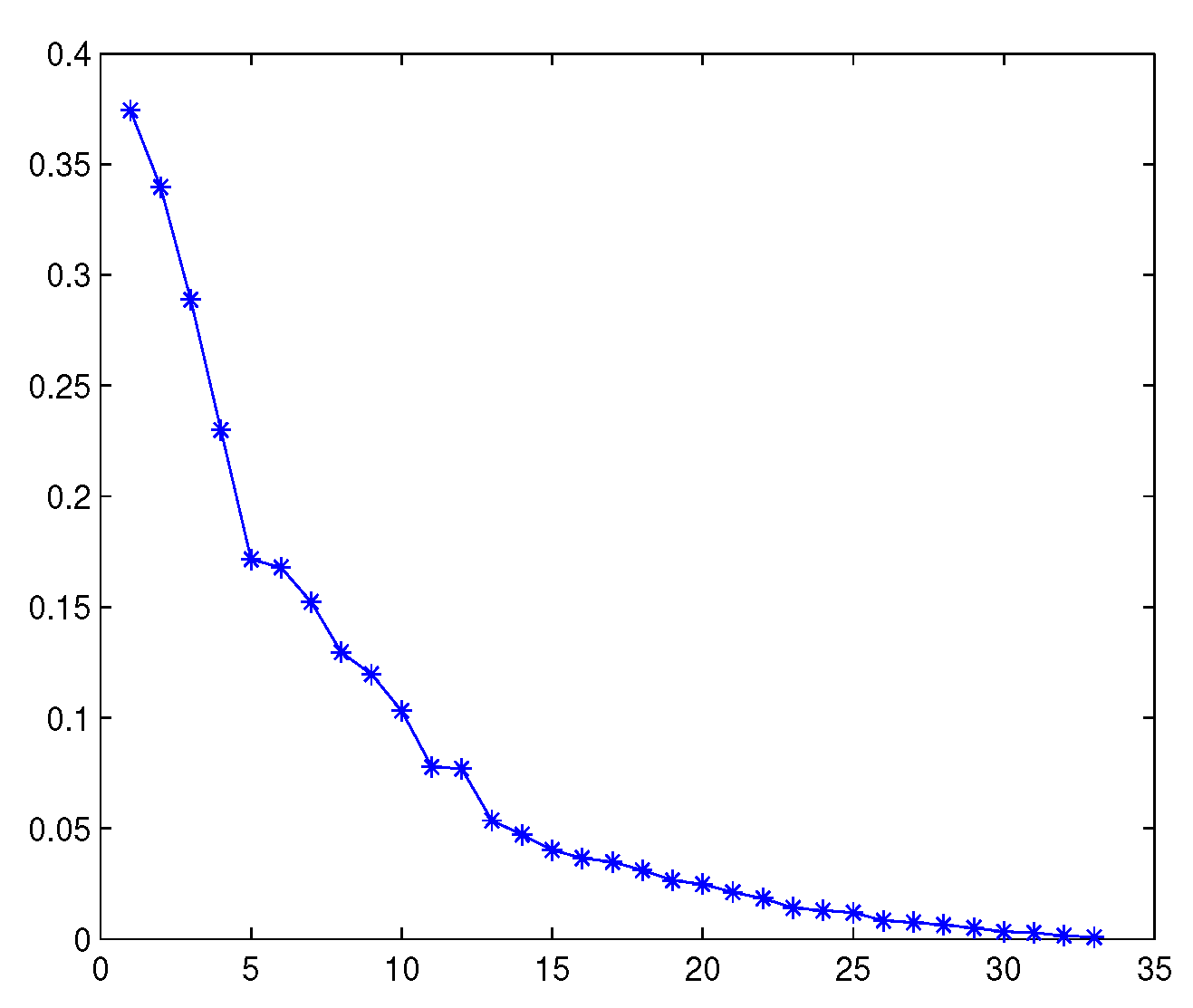
We consider two sets of correlation lengths in our numerical examples. In the first example, we take $l_1=0.1$, $l_2=0.4$, and ${\sigma }^2=2$ in a $50\times 50$ fine-scale grid. $\theta$’s are generated from a log-normal distribution. Eigenvalues decrease rapidly as shown in Figure 4.

The MCMC method with a random walk proposal of step-size $0.3$ is used to get samples from $\pi \left(\theta \right)$. A different number of K-L terms are taken into account. The chains are run for 10,000 iterations with the first 500 samples as the burn-in period. The Monte Carlo integration retaining all the terms in the discrete K-L expansion is considered to be the true value of $E_{\pi \left(\theta \right)}F\left(\theta \right)$. Samples with a different number of truncated terms are taken to compute $E_{\tilde{\pi }\left(\theta \right)}F\left(\theta \right)$ in different cases to compare with the true one.

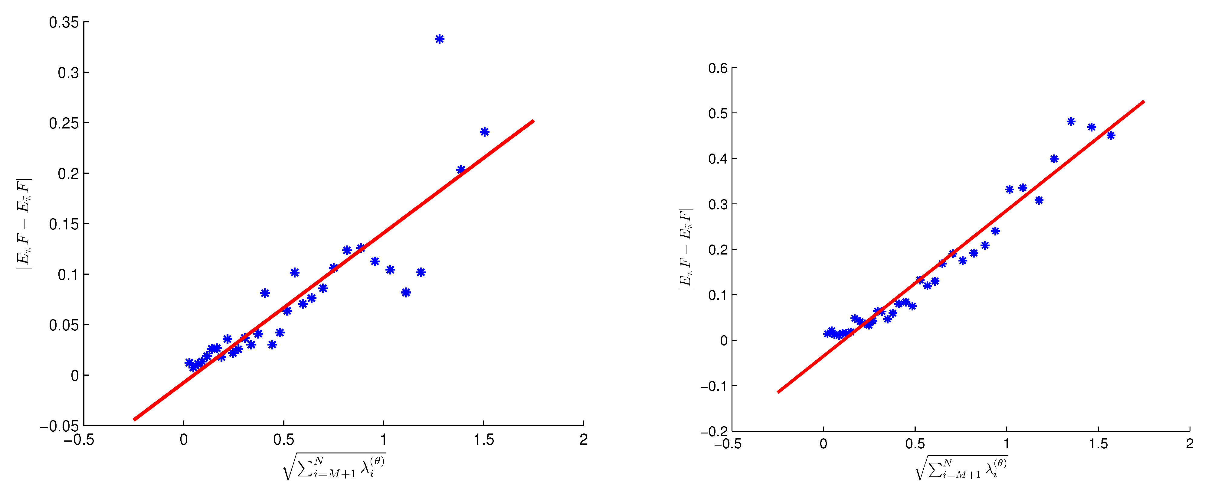
In the second example, we take the case with $l_1=l_2=0.2$ and ${\sigma }^2=2$. Table 1 and Table 2 show the results with a different number of truncated K-L terms M for the first and second example respectively. In both cases, the errors decrease with the same convergence rate related to the sum of eigenvalue remainders of $R\left(x\right)$. This can be observed more clearly from Figure 5, where the data sets $\{{\left({\sum }_{i=M+1}^N{\lambda }_i^{\left(\theta \right)}\right)}^{\frac{1}{2}},$ $|E_{\pi }F-E_{\tilde{\pi }}F\left|\right\}$ can be fitted as a straight line. Namely, the relationship between $|E_{\pi }F-E_{\tilde{\pi }}F|$ and ${\left({\sum }_{i=M+1}^N{\lambda }_i^{\left(\theta \right)}\right)}^{\frac{1}{2}}$ is linear as shown in Theorem 1, while ignoring the errors in computing $F\left(\theta \right)$.

5.1.2. Channelized Reservoirs

In our next example, we consider a permeability field with three facies. It is assumed that there is a high permeability layer in the middle and low permeability layers in the two ends. The corresponding two interfaces are chosen randomly with the condition that the upper facies boundary is always above the lower facies boundary. The two different channels are populated using two log-Gaussian random fields generated from truncated K-L expansions with two-point correlation function (23). The high permeable layer has correlation lengths $l_x=0.1$, $l_y=0.4$, and $\sigma =1$, and the low permeable layer has correlation lengths $l_x=l_y=0.2$, and $\sigma =0.4$. For both interfaces, a 1-d version of Equation (23) is used with correlation length $l=0.05$ and $\sigma =1.5$.

We take the generated permeability field as the reference, and run the forward model with one injector at $(0,0.5)$ and one producer at $(1,0.5)$ in this reference permeability field to get the fractional flow data $F_{obs}$. An MCMC chain is run for 10,000 iterations to get the posterior samples of the permeability field, with the first 500 samples as a burn-in period.

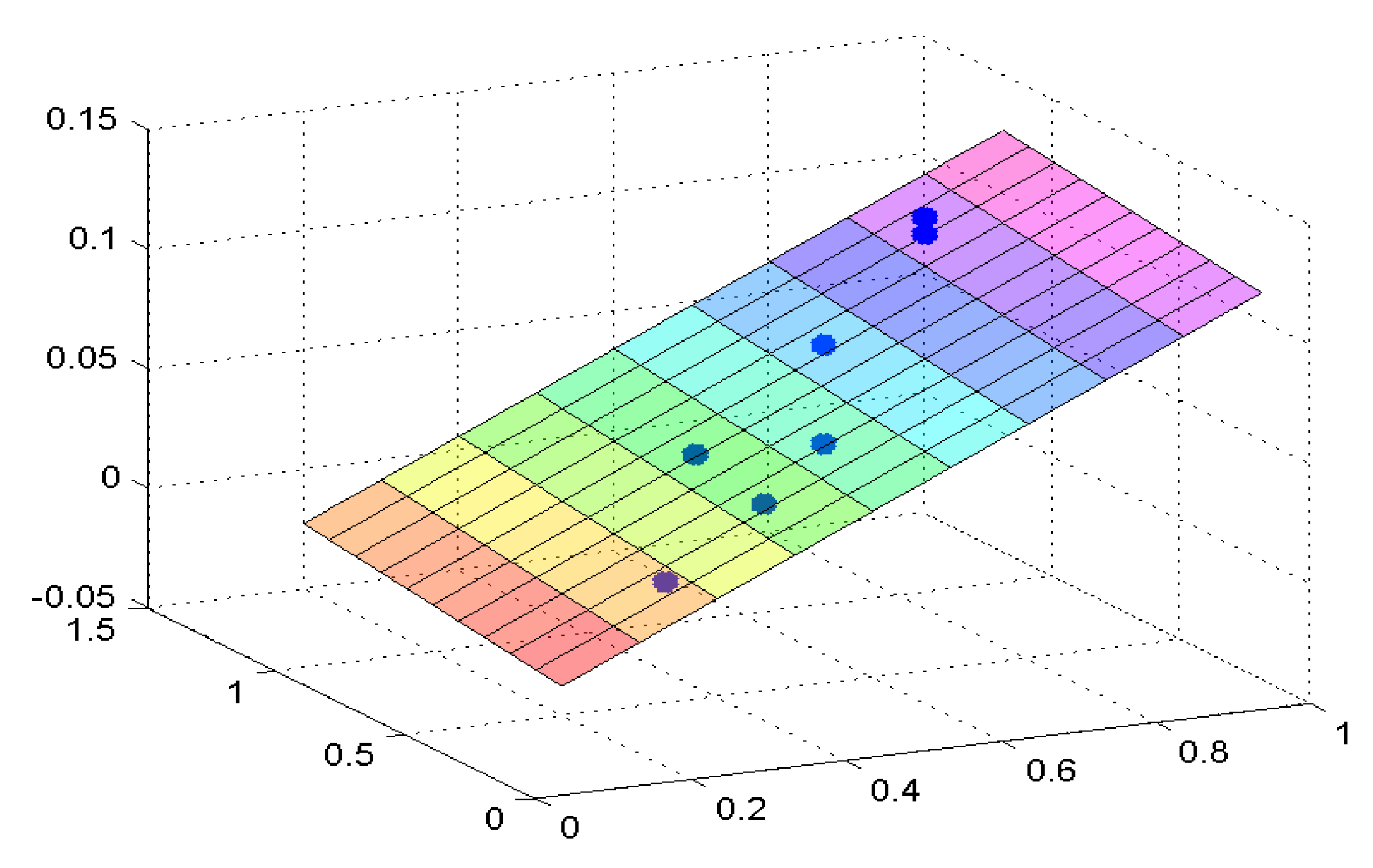
The estimations of posterior errors for a different number of terms in the truncations of K-L expansions, similar to Table 1 and Table 2, are reported in

Table 3. Posterior errors $|E_{\pi }F-E_{\tilde{\pi }}F|$ when the K-L expansion is truncated to M terms for different facies.

${\mathit{M}}_1$	${\mathit{M}}_2$	$\tilde{\mathit{M}}$	${\left({\sum }_{\mathit{j}={\mathit{M}}_1+1}^{{\mathit{N}}_1}{\mathit{\lambda }}_{1\mathit{j}}^{\left(\mathit{\theta }\right)}\right)}^{\frac{1}{2}}$	${\left({\sum }_{\mathit{j}={\mathit{M}}_2+1}^{{\mathit{N}}_2}{\mathit{\lambda }}_{2\mathit{j}}^{\left(\mathit{\theta }\right)}\right)}^{\frac{1}{2}}$	${\left({\sum }_{\mathit{i}=\tilde{\mathit{M}}+1}^{\tilde{\mathit{N}}}{\mathit{\lambda }}_{\mathit{i}}^{\left(\mathit{\alpha }\right)}\right)}^{\frac{1}{2}}$	$|{\mathit{E}}_{\mathit{\pi }}\mathit{F}-{\mathit{E}}_{\tilde{\mathit{\pi }}}\mathit{F}|$
5	5	5	0.526235	0.786077	0.853727	0.109464
10	5	5	0.367011	0.786077	0.853727	0.116172
10	10	10	0.367011	0.530798	0.477141	0.051925
15	10	10	0.253542	0.530798	0.477141	0.093109
15	15	10	0.253542	0.365967	0.477141	0.053869
20	15	15	0.169250	0.365967	0.210844	0.047356
20	20	15	0.169250	0.238932	0.210844	0.019996

. The Monte Carlo integration retaining all the terms in the discrete K-L expansions is considered to be the true value. In Table 3, we can see that the error between the true value and the estimated value from the truncated posterior decreases consistently as we increase the number of the terms retained in K-L expansion. If we further plot the errors, we can see that they lie on a plane (see Figure 6) as indicated in Theorem 2.

5.2. Matching Permeability with Reduced Parameters

In this example, we will show that the reference permeability field can be recovered from matching the observations and that the accuracy of such estimates is certainly affected by the truncation of expansions. We consider a high permeable layer in the middle and low permeable layers in the two ends with the same correlation lengths as in Section 5.1.2. The interfaces are taken as a linear interpolation of independent points.

In the first part, we truncate the K-L expansion and retain only the first 20 terms for the two permeability fields. We consider 25 points on the facies. So the dimension of $\theta$ is 40 and the dimension of $\alpha$ is 25. The two-stage MCMC method is used to sample from the posterior. The initial facies boundaries are taken to be straight lines joining the two ends of the known facies boundaries. We use random walks to perturb $\theta$ and $\alpha$ with step sizes $0.25$ and $0.05$, respectively, and with independent Gaussian priors for $\theta$ and $\alpha$. We run the MCMC chain for 10,000 iterations and leave out the first 500 samples as the burn-in period.

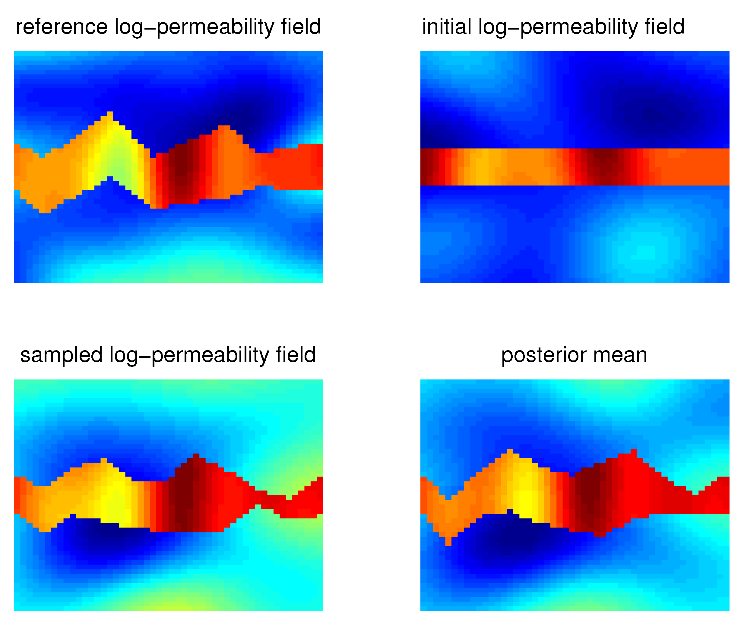
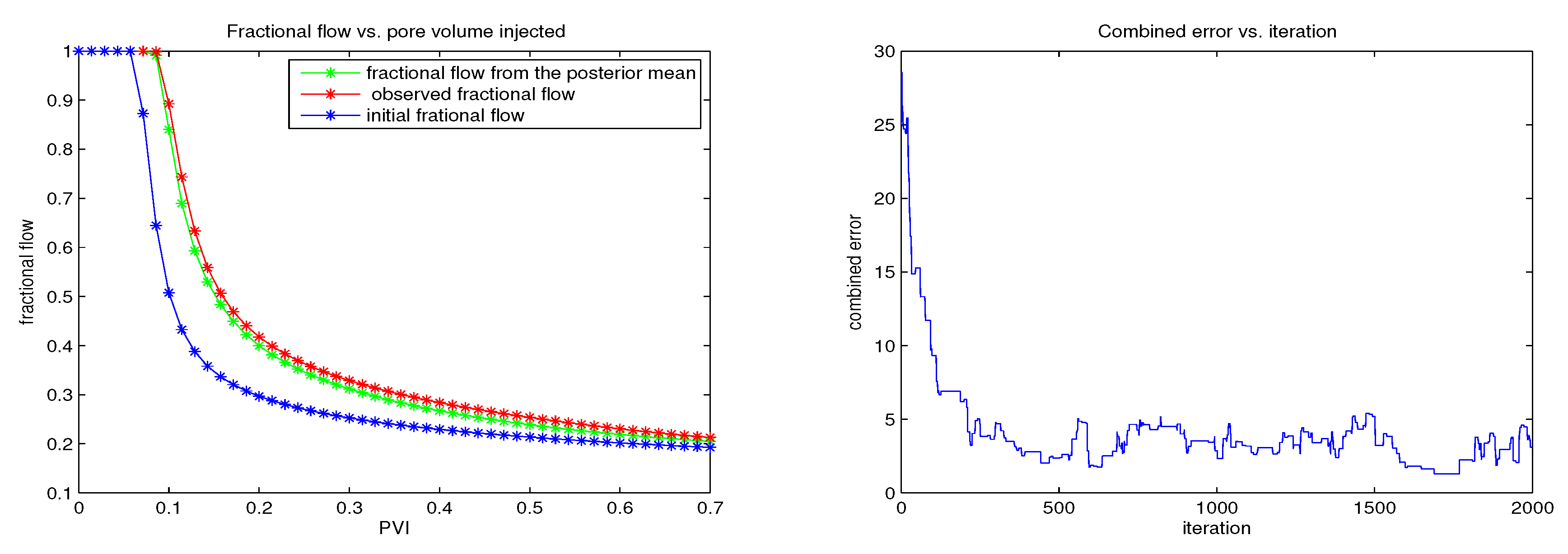
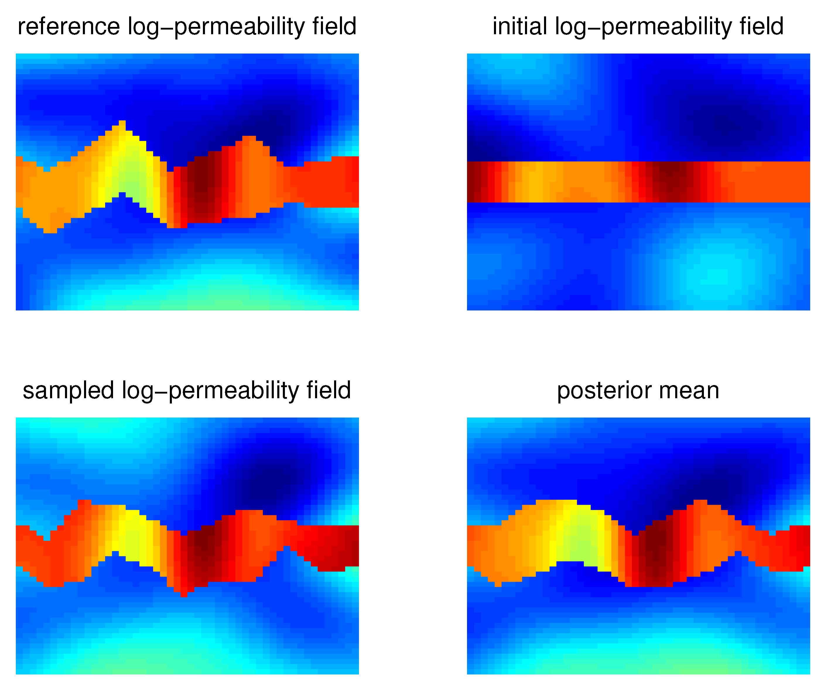
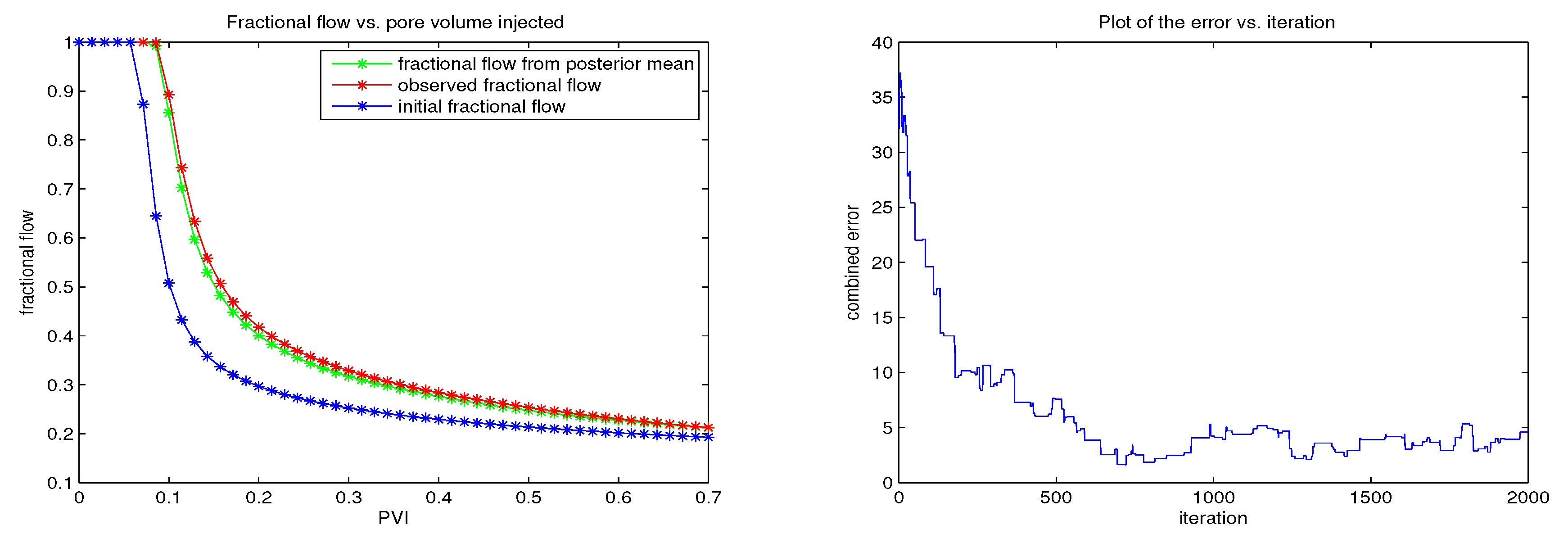
In Figure 7, the reference permeability field, the initial permeability field, and the mean of the posterior permeability field are shown. We can see that the sample mean is very close to the reference field. On the left plot of Figure 8 we can see that the sample estimate of the fractional flow of oil is quite close to the observed data. From the right plot of Figure 8 we can see that combined error decreases nearly to zero and stays there, which shows that the Markov chain has converged. The two-stage MCMC has a higher acceptance rate [32] (four times in these calculations) because it rejects the bad proposal quickly in the first stage, which is inexpensive. Next, we repeat the same procedure of sampling the posterior but we retain 25 terms in the K-L expansion for the two permeability fields. We use the same reference permeability field and the fractional flow of oil data. The numerical results are shown in Figure 9 and Figure 10. We can see the sampled mean of the permeability field is more accurate than the previous example with 20 K-L coefficients.

6. Conclusions

In this article, subsurface characterization for flows in highly heterogeneous porous media is studied. We consider channelized spatial fields to describe the permeability field where channel boundaries are assumed to have random locations and described via a level set approach. In particular, we use smooth velocity fields to change the channel boundaries within a level set framework and, thus, the parameterization of channel boundaries can be mapped to that of smooth velocity fields. This gives a reduced dimensional parameterization. Permeability distribution within each channel is assumed to be log-Gaussian and described via K-L expansion. One of our main contributions is the study of the regularity of posterior distribution. In particular, we study errors introduced in the posterior measure by truncating the prior distribution. The result from the theorem allows us to carry out the Bayesian uncertainty analysis in a finite-dimensional space. This makes the analysis easy and avoids involving “infinite” dimensional probabilistic spaces. We show that the posterior error introduced by truncation is bounded by a function of eigenvalues up to a constant, where this constant is independent of the dimension of the stochastic space. The latter guarantees that the truncation of K-L expansion based on a discretization will not introduce an unbounded error for the corresponding posterior distribution. The subsurface characterization within the Bayesian framework is based on the MCMC samples from the posterior distribution. We use an efficient two-stage MCMC that utilizes mixed MsFEM to screen the proposals. The numerical results show the validity of the proposed parameterization to interfaces and the error estimations.

One limitation of our study is that the results about the posterior error bounds are based on the assumptions that the saturation is a smooth field and permeability is a second-order stationary spatial process whose prior distribution is a Gaussian process. The complete set of assumptions are given in Appendix A. Although the stationarity assumption is quite reasonable for permeability description within facies boundaries, relaxing some of these assumptions could be beneficial for more complex reservoir models. In future, we would like to extend our Bayesian methodology for non-stationary permeability fields. Studying the posterior error bounds for non-Gaussian spatial processes and non-smooth velocity fields are also of interest for future research.

References

- Weber, K.J. Influence of Common Sedimentary Structures on Fluid Flow in Reservoir Models. J. Pet. Technol. 1990, 34, 665–672. [Google Scholar] [CrossRef]
- Dubrule, O. Geostatistics in Petroleum Geology; Course Note Series 38; American Association of Petroleum Geology: Tulsa, OK, USA, 1998. [Google Scholar]
- Haldorsen, H.; Damsleth, E. Stochastic Modeling. J. Pet. Technol. 1990, 42, 404–412. [Google Scholar] [CrossRef]
- Koltermann, C.E.; Gorelick, S.M. Heterogeneity in sedimentary deposits: A review of structure-imitating, process-imitating, and descriptive approaches. Water Resour. Res. 1996, 32, 2617–2658. [Google Scholar] [CrossRef]
- Egeland, T.; Georgsen, F.; Knarud, R.; More, H. Multifacies Modelling of Fluvial Reservoirs. In Proceedings of the SPE 26502 in proceedings of the SPE Annual Technical Conference and Exhibition, Houston, TX, USA, 3–6 October 1993. [Google Scholar]
- Caumon, G.; Strebelle, S.; Journel, J.C.A. Assessment of Global Uncertainty for Early Appraisal of Hydrocarbon Fields. In Proceedings of the SPE 89943, Annual Technical Conference and Exhibition, Houston, TX, USA, 26–29 September 2004. [Google Scholar]
- Caers, J. Petroleum Geostatistics; SPE Interdisciplinary Primer Series; Society of Petroleum Engineers: Richardson, TX, USA, 2006; 96p. [Google Scholar]
- Hubbard, S.S.; Rubin, Y.; Majer, E. Spatial correlation structure estimation using geophysical and hydrogeological data. Water Resour. Res. 1999, 35, 1809–1826. [Google Scholar] [CrossRef]
- Lee, H.; Higdon, D.; Bi, Z.; Ferreira, M.; West, M. Markov Random Field Models for High-Dimensional Parameters in Simulations of Fluid Flow in Porous Media. Technometrics 2002, 44, 230–241. [Google Scholar] [CrossRef]
- Oliver, D.S.; Reynolds, A.C.; Bi, Z.; Abacioglu, Y. Integration of production data into reservoir models. Pet. Geosci. 2001, 7, S65–S73. [Google Scholar] [CrossRef]
- Vasco, D.W.; Yoon, S.; Datta-Gupta, A. Integrating a Dynamic Data Into High Resolution Reservoir Models Using Streamline-Based Analytical SensitivityCoefficients. SPEJ 1999, 4, 389. [Google Scholar] [CrossRef]
- Wilson, A.; Rubin, Y. Characterization of aquifer heterogeneity using indicator variables for solute concentrations. Water Resour. Res. 2002, 38, 1283. [Google Scholar] [CrossRef]
- Akbarabadi, M.; Borges, M.; Jan, A.; Pereira, F.; Piri, M. A Bayesian framework for the validation of models for subsurface flows: Synthetic experiments. Comput. Geosci. 2015, 19, 1231–1250. [Google Scholar] [CrossRef]
- Iglesias1, M.A.; Lin, K.; Stuart, A.M. Well-posed Bayesian geometric inverse problems arising in subsurface flow. Inverse Probl. 2014, 30, 114001. [Google Scholar] [CrossRef] [Green Version]
- Mondal, A.; Efendiev, Y.; Mallick, B.; Datta-Gupta, A. Bayesian Uncertainty Quantification for Flows in Heterogeneous Porous Media using Reversible Jump Markov Chain Carlo Methods. Adv. Water Resour. 2010, 33, 241–256. [Google Scholar] [CrossRef]
- Mondal, A.; Mallick, B.; Efendiev, Y.; Datta-Gupta, A. Bayesian uncertainty quantification for subsurface inversion using a multiscale hierarchical model. Technometrics 2014, 56, 381–392. [Google Scholar] [CrossRef]
- Yang, K.; Guha, N.; Efendiev, Y.; Mallick, B.K. Bayesian and variational Bayesian approaches for flows in heterogeneous random media. J. Comput. Phys. 2017, 345, 275–293. [Google Scholar] [CrossRef] [Green Version]
- Bayat, M.; Kia, M.; Soltangharaei, V.; Ahmadi, H.R.; Ziehl, P. Bayesian demand model based seismic vulnerability assessment of a concrete girder bridge. Adv. Concr. Constr. 2020, 9, 337–343. [Google Scholar]
- Mangalathu, S.; Jeon, J.-S.; DesRoches, R.; Padgett, J. Application of Bayesian Methods to Probabilistic Seismic Demand Analyses of Concrete Box-Girder Bridges. Geotech. Struct. Eng. Congr. 2016, 1367–1379. [Google Scholar] [CrossRef]
- Osher, S.; Fedkiw, R. Level Set Methods and Dynamic Implicit Surfaces; Springer: New York, NY, USA, 2003. [Google Scholar]
- Osher, S.; Sethian, J.A. Front propogation with curvature dependent speed: Algorithms based on Hamilton-Jacobi formulations. J. Comp. Phys. 1988, 56, 12–49. [Google Scholar] [CrossRef] [Green Version]
- Sethian, J. Level Set Methods and Fast Marching Methods; Cambridge University Press: Cambridge, UK, 1999. [Google Scholar]
- Tai, X.C.; Chan, T. A survey on multiple level set methods with applications for identifying piecewise constant functions. Int. J. Numer. Anal. Model. 2004, 1, 25–47. [Google Scholar]
- Villegas, R.; Dorn, O.; Moscoso, M.; Kindelan, M. Simulations characterization of geological shapes and permeability distributions in reservoirs using the level set method. In Proceedings of the SPE 100291, SPE Europec/EAGE Annual Conference and Exhibition, Vienna, Austria, 12–15 June 2006. [Google Scholar]
- Durlofsky, L.J. Numerical calculations of equivalent gridblock permeability tensors for heterogeneous porous media. Water Resour. Res. 1991, 27, 699–708. [Google Scholar] [CrossRef] [Green Version]
- Aarnes, J.E. On the use of a mixed multiscale finite element method for greater flexibility and increased speed or imporved accuracy in reservoir simulation. SIAM MMS 2004, 2, 421–439. [Google Scholar] [CrossRef]
- Chen, Z.; Hou, T.Y. A mixed multiscale finite element method for elliptic problems with oscillating coefficients. Math. Comp. 2003, 72, 541–576. [Google Scholar] [CrossRef] [Green Version]
- Efendiev, Y.; Hou, T.Y. Multiscale Finite Element Methods: Theory and Applications; Springer: Berlin, Germany, 2009. [Google Scholar]
- Wong, E. Stochastic Processes in Information and Dynamical Systems; MCGraw-Hill: New York, NY, USA, 1971. [Google Scholar]
- Schwab, C.; Todor, R. Karhunen-Loève approximation of random fields by generalized fast multipole methods. J. Comput. Phys. 2006, 217, 100–122. [Google Scholar] [CrossRef]
- Robert, C.; Casella, G. Monte Carlo Statistical Methods; Springer: New York, NY, USA, 1999. [Google Scholar]
- Efendiev, Y.; Hou, T.; Luo, W. Preconditioning of MCMC simulations using coarse-scale models. SIAM Sci. Comp. 2006, 28, 776–803. [Google Scholar] [CrossRef]
- Strinopoulos, T. Upscaling Immiscible Two-Phase Flows in an Adaptive Frame. Ph.D. Thesis, California Institute of Technology, Pasadena, CA, USA, 2005. [Google Scholar]
Figure 1.
Illustration of the permeability field with facies.
Figure 2.
Interface evolution by moving initial interface with different vertical velocity fields.
Figure 3.
Interface updates using velocity representation at some fixed points.
Figure 4.
Ordered eigenvalues for , , and .
Figure 5.
Linear fit of . Left: , , , and ; Right: , , , and .
Figure 6.
Plots of .
Figure 7.
Top left: The true log-permeability field. Top right: Initial log-permeability field. Bottom left: One of the sampled log-permeability field. Bottom Right: The mean of the sampled log-permeability field from two-stage MCMC using 20 K-L terms.
Figure 8.
Left: Red line designates the fine-scale reference fractional flow of oil, the blue line designates the initial fractional flow of oil, and the green line designates fractional flow of oil corresponding to mean of the sampled permeability field from two-stage MCMC. Right: Fractional flow errors vs. accepted iterations when sampled from the posterior distribution retaining 20 terms in K-L expansion.
Figure 9.
Top left: The true log-permeability field. Top right: Initial log-permeability field. Bottom left: One of the sampled log-permeability field. Bottom Right: The mean of the sampled log-permeability field from two-stage MCMC using 25 K-L terms.
Figure 10.
Left: Red line designates the fine-scale reference fractional flow of oil, the blue line designates the initial fractional flow of oil, and the green line designates fractional flow of oil corresponding to mean of the sampled permeability field from two-stage MCMC. Right: Fractional flow errors vs. accepted iterations when sampled from the posterior distribution retaining 25 terms in K-L expansion.